

Development of Technology for Identification of Climate Patterns during Floods Using Global Climate Model Data with Convolutional Neural Networks

1
Department of Hydro Science and Engineering Research, Korea Institute of Civil Engineering and Building Technology, Goyang 10223, Republic of Korea
2
Department of Civil Engineering, Chosun University, Gwangju 61452, Republic of Korea
*
Authors to whom correspondence should be addressed.
Water 2022, 14(24), 4045; https://doi.org/10.3390/w14244045
Submission received: 21 October 2022
/
Revised: 6 December 2022
/
Accepted: 7 December 2022
/
Published: 12 December 2022
(This article belongs to the Special Issue A Safer Future—Prediction of Water-Related Disasters)
Abstract
:Given the increasing climate variability, it is becoming difficult to predict flooding events. We may be able to manage or even prevent floods if detecting global climate patterns, which affect flood occurrence, and using them to make predictions are possible. In this study, we developed a deep learning-based model to learn climate patterns during floods and determine flood-induced climate patterns using a convolutional neural network. We used sea surface temperature anomaly as the learning data, after classifying them into four cases according to the spatial extent. The flood-induced climate pattern identification model showed an accuracy of ≥89.6% in all cases, indicating its application for the determination of patterns. The obtained results can help predict floods by recognizing climate patterns of flood precursors and be insightful to international cooperation projects based on global climate data.
1. Introduction
Heavy rains caused by extreme climates result in floods in worldwide. Although several studies aiming to predict such floods occurrences, the climate variability and uncertainty makes such predictions and subsequent preparations difficult. If we are able to forecast the occurrence of floods through the climatic factors affecting them, we can effectively prepare for the incoming damage [1,2,3,4,5]. For example, for the El Niño (La Niña) phenomenon, a major global event, climate information is provided through sea surface temperature anomalies within the monitoring zone in the tropical Pacific Ocean (5° S to 5° N, 170° W to 120° W). This event is well known for causing massive floods, particularly across South Asia and Australia [6]. Also, recently, an unprecedented flood occurred in Pakistan for the second consecutive year. Given the occurrence of these floods, several studies have been conducted using El Niño (La Niña) projections for climate prediction.
The relationship between various global climate factors and climate patterns have been studied globally [7,8,9,10,11,12,13,14]. For example, Nurutami and Hidayat (2016) analyzed the effects of the Indian Ocean dipole (IOD), El Niño-Southern Oscillation (ENSO), and sea surface temperature (SST) on seasonal rainfall changes in Indonesia [15]. They confirmed a clear association between climate patterns, SST, and rainfall patterns and proposed a method to more accurately analyze the highly variable rainfall patterns in Indonesia.
The effects of climate factors on the occurrence of extreme hydrological events (i.e., floods and droughts) have been extensively studied [16,17,18,19,20]. Fang et al. (2021) found a correlation between spatiotemporal variability of droughts and various climatic factors in Central and East China [21]. Specifically, they found that the variability of droughts in the spring and winter was related to different climatic factors and concluded that identifying them can contribute to efficient water resource management and improve the accuracy of drought early warning systems. In addition, Tong et al. (2005) analyzed the correlation between ENSO and the occurrence of floods and droughts in the Yangtze River—one of the most representative rivers of China [22]. They found strong correlations between flooding and El Niño and between droughts and La Niña in the lower reaches of the river. Wu et al. (2020) used Pearson-correlation coefficients and the cross-wavelet transform method to investigate the correlation between hydrological droughts and various climatic factors [23]. They found that two climatic factors, namely, ENSO and Pacific Decadal Oscillation (PDO), had a strong relationship with the hydrological drought index which is called as Streamflow Index. In addition, an intra-annual and inter-decadal relationship between the Streamflow Index and ENSO was observed, showing a clear causal relationship between the hydrological drought phenomenon and climatic factors.
Machine learning is a technique mainly used for classification, regression, and predictive problems based on relationships between data. In other words, it combines and analyzes external data based on relationships between data “learned” by the computer. Since the 1990s, the development of data observation systems and the improvement of big data technology have enabled the scope of machine learning to rapidly expand. Deep learning, a field of machine learning, involves connecting artificial neural networks, one of the representative machine-learning technologies, in the form of numerous layers. Deep-learning techniques are often used in image analysis, prediction of time series data, and language translation [24,25,26,27,28].
In hydrology, research is being actively conducted using machine learning and deep learning is also actively underway. In general, these techniques have been used for developing rainfall-runoff models or for temporal predictions of various hydrological factors. More recently, hydrological analysis with grid-based image data has been conducted using advanced deep-learning technologies [29,30]. Using machine learning or deep learning technology, it is possible to identify how various climate factors are related to the occurrence of floods and droughts in different regions; specific methods are being developed for the prediction of such adverse events according to changes in climate factors. Tian et al. (2018) used two representative climate indices, ENSO and western Pacific subtropical high, to improve the prediction accuracy of agricultural droughts in the Xiangjing River Basin in China [31]. The authors used a machine learning technique (called the support vector regression model; SVR) for prediction and confirmed that prediction accuracy increased when the western Pacific subtropical high index was used as an indicator. Li et al. (2021) used three machine learning techniques—support vector regression (SVR), random forest (RF), and extreme learning machine (ELM)—to analyze how the changing patterns of SST can act as a predictor for drought in the central United States [32]. They suggested that drought predictions based on the ELM model showed high accuracy and can therefore be used as a tool for drought prediction and early warning system construction.
In this study, we applied deep-learning techniques (i.e., Convolution Neural Network) to identify the global climate patterns that affect flood occurrence in the Korean peninsula. Flood-induced climate pattern (i.e., sea surface temperature anomaly) was used to describe a climate pattern affecting flood occurrence. If the flood-induced climate pattern affecting the occurrence of floods was observed in the model, we considered that mid- to long-term flood predictions can be made based on the obtained pattern.
2. Methods
2.1. Study Area and Data Collection
2.1.1. Study Area
In this study, the Korean peninsula was selected as study site. The Korean peninsula is located in the middle latitude on the western boundary of the North Pacific Ocean (33–43° N and 124–132° E). The extreme domestic climate, including floods, is affected by circumglobal teleconnection (CGT) patterns, such as the Pacific sea level and temperature deviations, including the El Niño phenomenon [4,33]. However, as the peninsula is located in a mid-latitude region and is affected by complex climate factors, its correlation with the known climate index is low. We therefore intended to identify the CGT pattern affecting the occurrence of domestic floods, by applying deep-learning techniques.
2.1.2. Definition of Flood Events
To build a deep-learning-based classification model, we first defined flood events from 1982 to 2021. Data on the extent of large-scale flood damage by period in Korea [34], nationwide precipitation statistics [35], and flood alert (watch and warning) information [36] from four flood control centers (Han River, Nakdong River, Geum River, and Yeongsan River) were collected. We defined flood occurrence based on three criteria: (1) large-scale flood damage, (2) monthly precipitation deviation of >100 mm, and (3) flood warnings or watches issued at three or more points during the flood season from June to September.
Among the data for 4880 days from June to September during 1982–2021, 1830 days were classified as flooding (37.5%) and 3050 days were classified as non-flooding (62.5%) days. To develop the classification model, there should not be a large difference in the ratio of flood occurrence to non-occurrence days; therefore, to match this ratio, data for flood non-occurrence days were selected at random.
2.1.3. Climate Data
To identify climate patterns affecting the occurrence of floods, we used sea surface temperature anomaly (SSTA) data, which are known to affect domestic precipitation, for analysis. Data provided from the U.S. National Oceanic and Atmospheric Administration National Climatic Data Center (NOAA NCDC), OISST AVHRR anom/SSTA (Optimum Interpolation 1/4 Degree Daily Sea Surface Temperature Anomaly Analysis version 2.1) were collected and analyzed [37,38,39]. These data are global ocean analysis data with a 0.25° × 0.25° grid resolution and are relevant from September 1981 until June 2022. For the analysis, data from the flood period of June to September during the period 1 January 1982–31 December 2021 were used.
In the case of spatial scope, four cases (Cases 1–4) were formed to compare and review the applicability of the classification model when constructing the classification model (Table 1 and Figure 1). For Cases 2–4, a relatively coarse grid was used by reducing the number of parameters constituting the model and lowering the resolution of the data to 2.5° × 2.5° to find the CGT pattern [40,41].
2.2. CNN Model Construction
2.2.1. CNN Model Structure
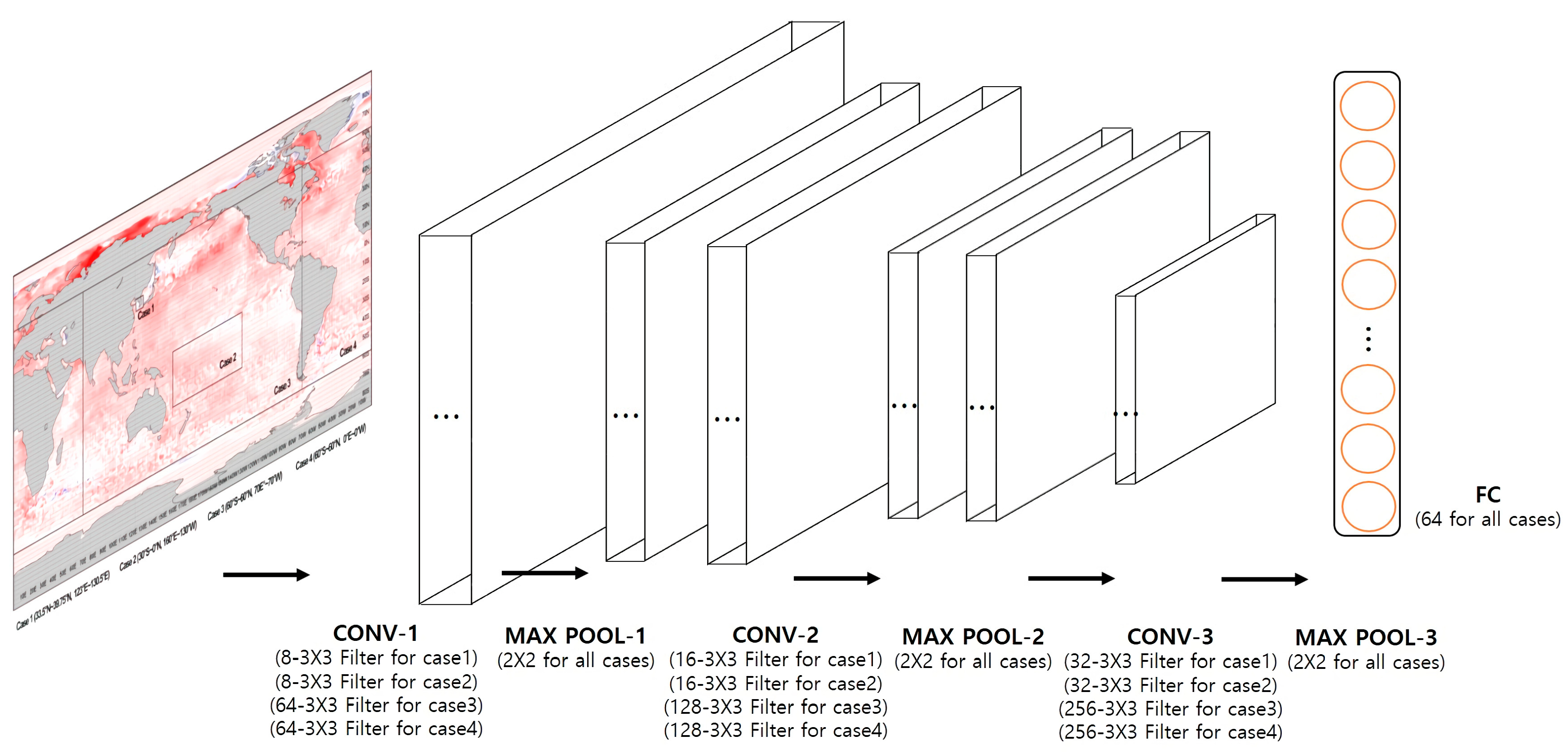
Deep learning is an upgraded method over the existing machine learning-based techniques. Deep learning, like machine learning, is effective for analyzing patterns within vast datasets based on complex and non-linear relationships. The CNN model is a deep-learning model based on the data-driven approach mainly used for image classification. As shown in Figure 2, the CNN model, which was used to create a classification model by extracting the features of two-dimensional data, was applied to further develop a model for determining global flood-induced climate patterns.
The CNN model has previously shown good performance, mainly in the context of image-based classification. This is because learning is performed while maintaining the spatial information of the image using convolutional filters—one of the defining characteristics of CNN [42,43,44]. The CNN model primarily consists of three layers: a convolutional layer, a pooling layer, and a fully connected layer. After the convolutional and pooling layers are repeatedly constructed, classification is performed through the fully connected layer and the activation function. The activation function exists between the layers and plays a role in facilitating learning as well as in determining the shape of the output value. Generally, the main types of activation functions are Sigmoid, Softmax, and Relu functions. CNN model learning is performed through this process, and recently, new models, such as VGGNet and ResNet, have been developed that mix additional ideas based on CNN.
2.2.2. Establishment of a Model to Identify Flood-Induced Climate Patterns
To construct a model for determining flood-induced climate patterns, it is necessary to analyze patterns from global climate data and to subsequently determine flood-inducing patterns using the obtained results. We analyzed climate patterns in the global climate model using a CNN-based deep-learning algorithm that could analyze images effectively. For this study, a CNN model for image classification was constructed using Python packages (Keras). The CNN model consisted of an input layer, three convolutional layers, three pooling layers, one fully connected layer, and one output layer. For model optimization, the structure and hyperparameters of each layer were determined through trial and error. Each convolutional layer used a 3 × 3 convolution filter, each pooling layer had a maximum pooling layer of 2 × 2, and the fully connected layer consisted of 64 nodes (Figure 2). ReLu and Softmax were used as activation functions, with a batch size of 64. Training was performed for a maximum of 100 epochs. In this study, the training period used in CNN model was from 1982 to 2006 and the model validating period was from 2007 to 2021.
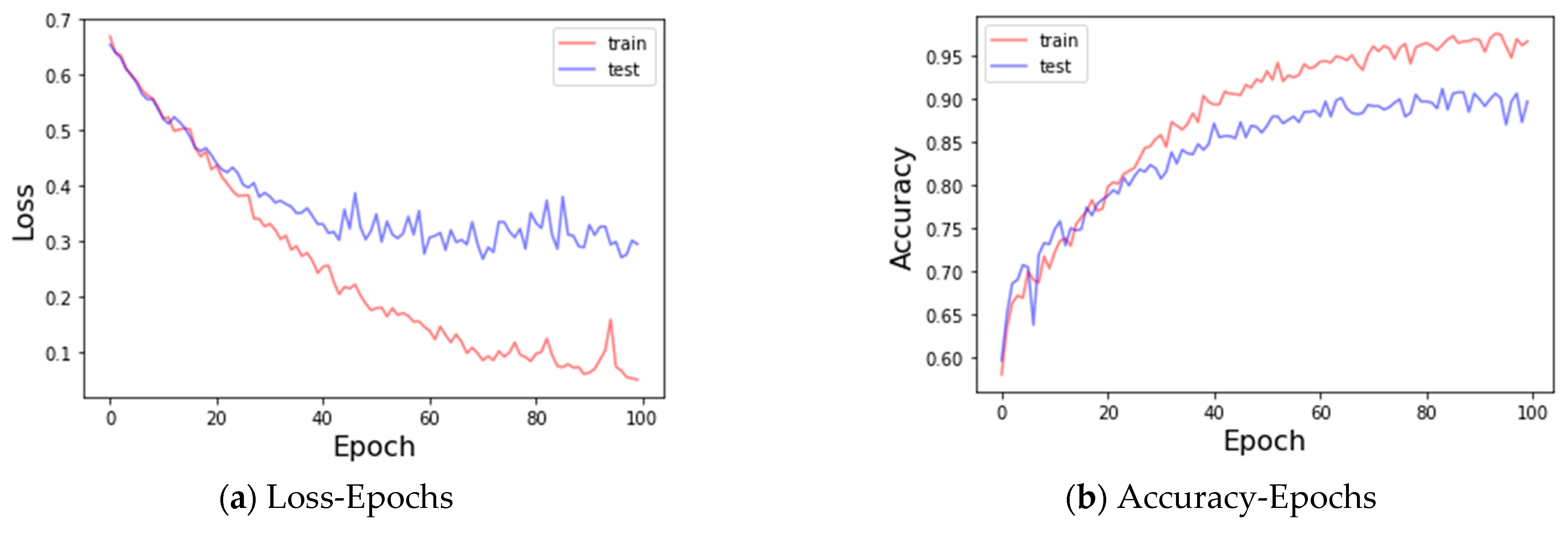
Figure 3 shows the loss and accuracy that occurred during training and validating as the epoch increases. For both training and validating, as the epoch increased, the loss decreased, and the accuracy increased simultaneously. This confirmed that the model was built correctly without overfitting.
2.2.3. Model Performance Evaluation Index
A confusion matrix, the most common method for performance evaluation of predictive models that perform binary classification and where the obtained results can be verified with various indicators through the combination of error matrices, was used in the study. An actual occurrence was categorized as True (1) and a non-occurrence as False (0). Actual occurrences predicted as 1 were called True Positives (TPs), actual occurrences predicted as 0 were called False Negatives (FNs), non-occurrences predicted as 1 were called False Positives (FPs), and non-occurrences predicted as 0 were called True Negatives (TNs) (Table 2).
The performance of the model was evaluated using precision, recall, specificity, accuracy, and the F1 score(Table 3). Precision, also referred to as the positive predictive value (PPV), is defined as the proportion of predictions that are predicted to occur. Recall, also called sensitivity, refers to the proportion of events that have occurred. Specificity refers to the proportion of correctly predicted events among events that did not occur, and accuracy is the proportion of correctly predicted events among all events. A high value in just one of the parameters precision, recall, or specificity does not necessarily mean the prediction performance is good. For example, model evaluation can be biased if only the recall for predicting actual occurrences and the specificity for predicting non-occurrences are considered [45]. In the case of accuracy, this bias can be reduced, but accurate performance evaluation is difficult when there is an imbalance between True and False values. The F1 score is an index that presents the harmonic average of precision and recall and is effective when there is an imbalance between True and False values.
3. Results
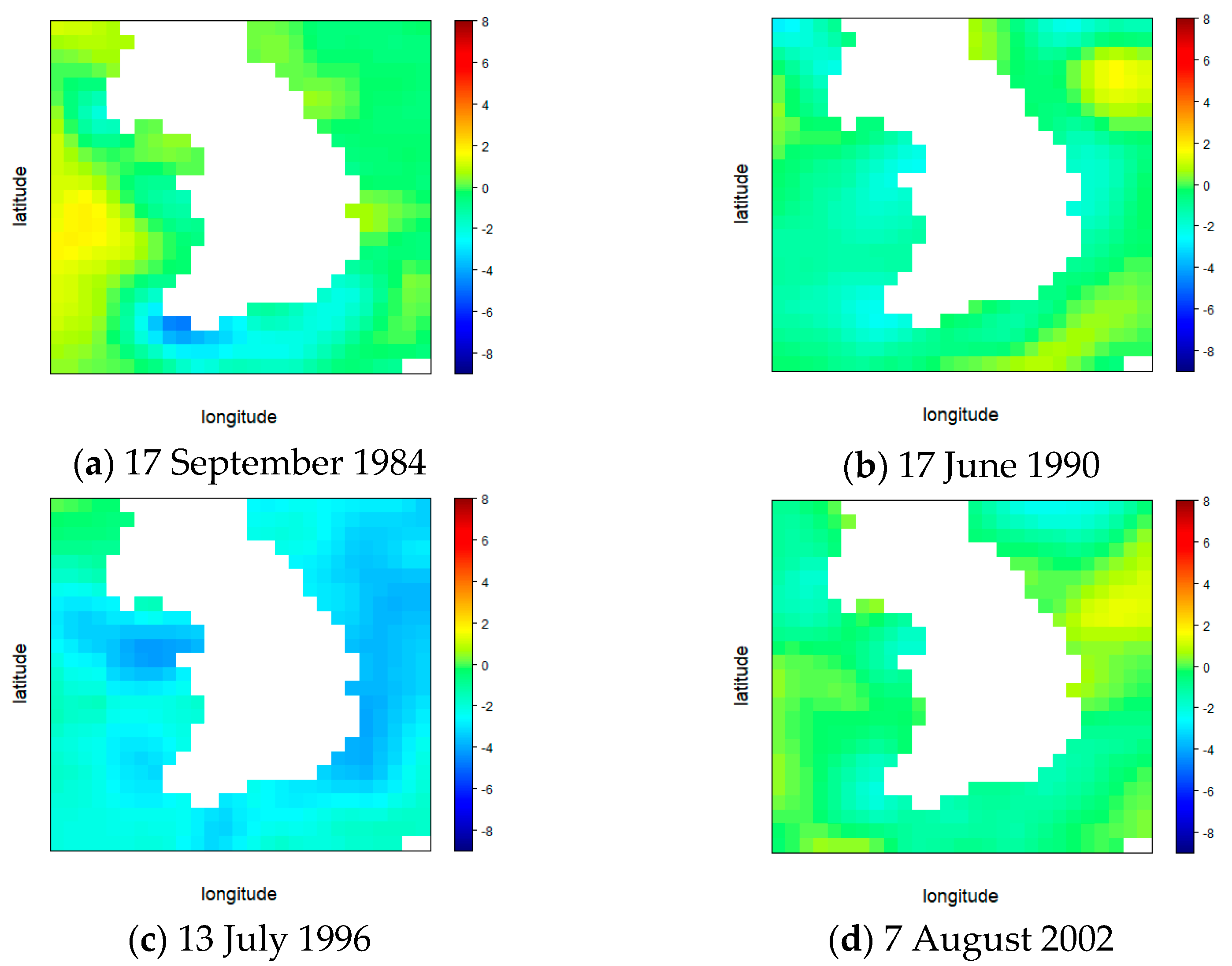
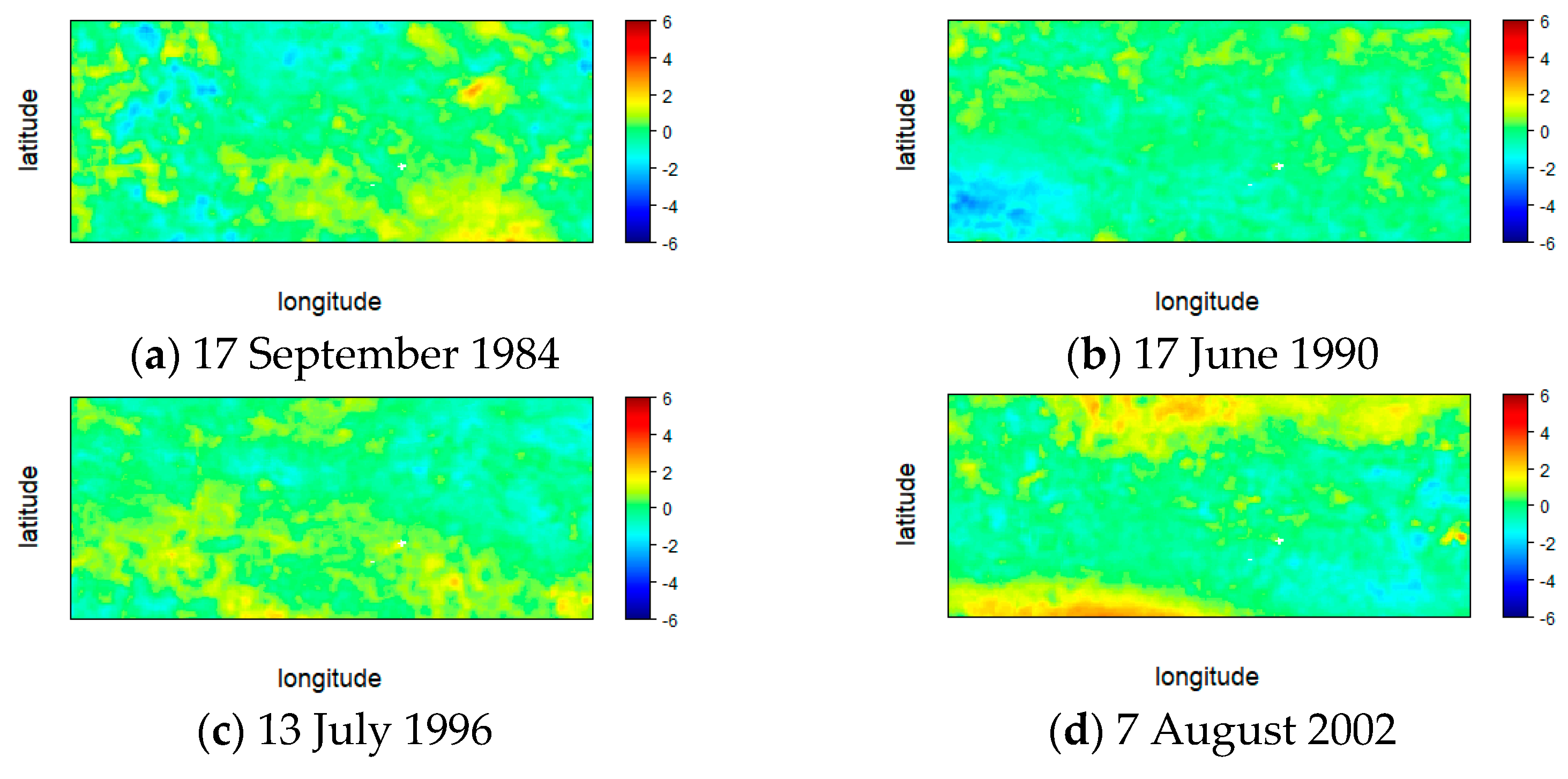
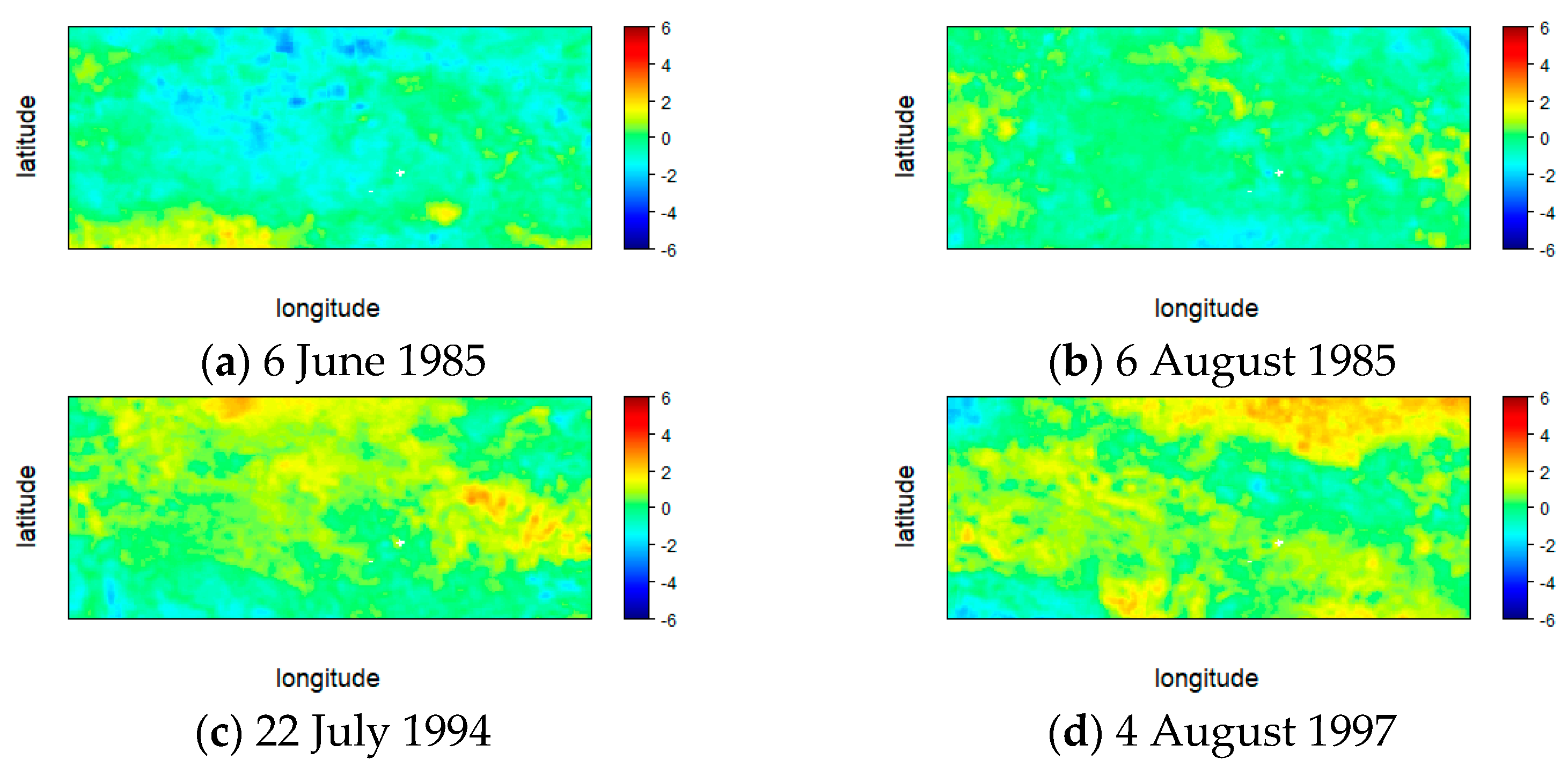
The spatial range and resolution of the SSTA data were classified into four cases, and subsequently, a model was developed to determine the climate patterns of flooding occurrence and flooding non-occurrence. As a result of classifying the flood occurrence and non-occurrence days of the climate pattern identification model for each case, the case where all four models were correct was 46.6% of the total number of tests when a flood occurred. When the flood did not occur, the case of fitting all four models was found to be 39.2% of the total number of tests. Comparing some of the sea surface temperature anomaly data when all four models are matched, it is shown in Figure 4, Figure 5, Figure 6, Figure 7, Figure 8 and Figure 9 below. Figure 4 shows the global sea surface temperature anomaly when all four model correct to classify flood occurrences, Figure 5 shows when all the results are correct that there is no flood. Figure 6 and Figure 7 and Figure 8 and Figure 9 show the spatial extent of Case 1 and Case 2, respectively. In case 1, which has a small spatial range, the difference in sea surface temperature anomaly is clearly distinguished, and in general, it can be seen that when the sea surface temperature of the neighboring sea is lower than the average year (blue), it is classified as a flood occurrence day, and when the sea surface temperature is higher (red), it is classified as a non-flood day. In case 2, a temperature pattern according to ocean currents appeared, and the number of cases in the pattern increased (Figure 6 and Figure 7). The flood occurred when the sea surface temperature in the lower left part was low or the temperature in the middle part was low. It can be seen that flooding did not occur when the sea surface temperature was generally lower than the average year and when the sea surface temperature in the central diagonal part was high (Figure 8 and Figure 9). In Cases 3 and 4, the spatial range was wide, so it was expressed as a global range. Although it was difficult to interpret with the naked eye because the number of occurrence patterns was too large, it can be seen that various large-scale climate patterns are appearing including El Niño and La Niña phenomenon.
To evaluate the performance of this model, an error matrix was presented for each case, and precision, recall, accuracy, specificity, and the F1 score were calculated using this matrix (Table 4 and Table 5). These tables represent classification results based on validation data after model training.
As shown in Table 5, the precision was 0.87 for Case 1, 0.94 for Case 2, 0.96 for Case 3, and 0.97 for Case 4 (range, 0.87–0.97). The recall was 0.94 for Case 1, 0.99 for Case 2, 0.98 for Case 3, and 0.99 for Case 4 (range, 0.94–0.99). The specificity was 0.85 for Case 1, 0.93 for Case 2, 0.96 for Case 3, and 0.96 for Case 4 (range, 0.85–0.96). The accuracy was 89.6% for Case 1, 96.1% for Case 2, 97.2% for Case 3, and 97.6% for Case 4 (range, 89.6–97.6%). Finally, the F1 score calculated using precision and recall was 0.90 for Case 1, 0.96 for Case 2, 0.97 for Case 3, and 0.98 for Case 4, indicating that the overall performance was good (range, 0.90–0.98). Overall, from Case 1 to Case 4, the larger the spatial range of the learning material, the better the performance.
These results show that the wider the spatial range, the more climate patterns that affect the occurrence of floods can be considered. This suggests a teleconnection between the local climate and a wide range of other climates. If the spatial range of the learning materials is narrow, the effect of teleconnection cannot be considered, and various climatic patterns, such as solar thermal energy and changes in local and temporary sea levels because of temperature change, are detected in addition to flood-inducing patterns resulting from complex factors. Therefore, the accuracy of flood identification of the developed was relatively low.
4. Conclusions
In this study, we developed a model to determine the occurrence of floods using SSTA data of past flooding events. The results from the flood-induced climate pattern identification model were evaluated by classifying the SSTA (that is, learning) data into four cases according to their spatial range. As the identification accuracy was >89.6%, we validated the applicability of our CNN-based method for determining flood-induced climate patterns.
Our study was different from previous ones that analyzed climate teleconnection through time series values of global climate data or climate index values. However, since our model uses binary classification that simply determines whether or not a flood occurs, the location or intensity of the flood could not be identified. In addition, as the time preceding the flood event is not considered, the preceding climate pattern that causes flooding could not be determined. Further studies expanded the present one are warranted to develop a model that can classify flood occurrence area, type, and intensity while considering the length of time preceding the flood event. Along the lines of the present study, we suggest the following future scalable studies:
- (1)
- The goal of this study was to develop a model that categorizes climate patterns during flooding, without considering the length of time preceding the flood. Future studies are warranted to build a prediction model for leading times (estimated 1–6 months) to use for flood preparation.
- (2)
- This study can be extended to research into dynamic causes of flood-induced climate patterns and analysis of the characteristics of each climate pattern change in the case of floods by water systems or points in detail.
- (3)
- We strongly suggest the study to be expanded to propose teleconnection climate indices induced by the extreme climate in Korea.
Although this study determines the climate pattern during flooding, we anticipate that it can be used to predict floods in advance by recognizing previous climate patterns preceding flooding. In addition, the results of this study have scientific and technological significance in terms of improving climate analysis technology, especially in other countries located at mid-latitudes where climate prediction is difficult, as well as contributing to resolving the global issue of water disasters.
Author Contributions
J.J. analyzed and interpreted the GCM data. H.H. supervised and was a major contributor in writing the manuscript. All authors have read and agreed to the published version of the manuscript.
Funding
Research for this paper was carried out under the KICT Research Program (project no. 20220175-001, Development of future-leading technologies solving water crisis against to water disasters affected by climate change) funded by the Ministry of Science and ICT.
Data Availability Statement
The data and materials that support the findings of this study are available on request from the corresponding author.
Acknowledgments
Research for this paper was carried out under the KICT Research Program (project no. 20220175-001, Development of future-leading technologies solving water crisis against to water disasters affected by climate change) funded by the Ministry of Science and ICT.
Conflicts of Interest
The authors declare that they have no known competing financial interest of personal relationships that could have appeared to influence the work reported in this paper.
Abbreviations
| CGT | Circumglobal teleconnection |
| CNN | Convolutional neural network |
| DOISST | Daily optimum interpolation sea surface temperature |
| ELM | Extreme learning machine |
| ENSO | El Niño-Southern Oscillation |
| FN | False Negative |
| FP | False Positive |
| IOD | Indian Ocean dipole |
| NAO | North Atlantic Oscillation |
| NOAA | National Oceanic and Atmospheric Administration |
| PDO | Pacific Decadal Oscillation |
| PPV | Rred to as the positive predictive value |
| RF | Random forest |
| SST | Sea surface temperature |
| SSTA | Sea surface temperature anomaly |
| SVR | Support vector regression |
| TN | True Negative |
| TP | True Positive |
References
- Cai, W.; Van Rensch, P.; Cowan, T.; Hendon, H.H. Teleconnection pathways of ENSO and the IOD and the mechanisms for impacts on Australian rainfall. J. Clim. 2011, 24, 3910–3923. [Google Scholar] [CrossRef]
- Lee, H.S. General rainfall patterns in Indonesia and the potential impacts of local season rainfall intensity. Water 2015, 7, 1751–1769. [Google Scholar] [CrossRef]
- Cho, J.P.; Jung, I.W.; Kim, C.G.; Kim, T.G. One-month lead dam infow forecast using climate indices based on teleconnection. J. Korea Water Resour. Assoc. 2016, 49, 361–372. [Google Scholar] [CrossRef]
- Lee, J.H.; Julien, P.Y. ENSO impacts on temperature over South Korea. Int. J. Climatol. 2016, 36, 3651–3663. [Google Scholar] [CrossRef]
- Cao, Q.; Hao, Z.; Yuan, F.; Su, Z.; Berndtsson, R.; Hao, J.; Nyima, T. Impact of ENSO regimes on developing- and decaying-phase precipitation during rainy season in China. Hydrol. Earth Syst. Sci. 2017, 21, 5415–5426. [Google Scholar] [CrossRef] [Green Version]
- Levin, N.; Phinn, S. Assessing the 2022 Flood Impacts in Queensland Combining Daytime and Nighttime Optical and Imaging Radar Data. Remote Sens. 2022, 14, 5009. [Google Scholar] [CrossRef]
- Gerlitz, L.; Vorogushyn, S.; Apel, H.; Gafurov, A.; Unger-Shayesteh, K.; Merz, B. A Statistically based seasonal precipitation forecast model with automatic predictor selection and its application to central and south Asia. Hydrol. Earth Syst. Sci. 2016, 20, 4605–4623. [Google Scholar] [CrossRef] [Green Version]
- He, S.; Wang, H. Impact of the November/December Arctic oscillation on the following January temperature in East Asia. J. Geophys. Res. Atmos. 2013, 118, 12981–12998. [Google Scholar] [CrossRef]
- He, S.; Gao, Y.; Li, F.; Wang, H.; He, Y. Impact of Arctic oscillation on the East Asian climate: A review. Earth Sci. Rev. 2017, 164, 48–62. [Google Scholar] [CrossRef] [Green Version]
- Kim, H.J.; Ahn, J.B. Possible impact of the autumnal North Pacifc SST and November AO on the East Asian winter temperature. J. Geophys. Res. Atmos. 2012, 117, D12. [Google Scholar] [CrossRef]
- Ouyang, R.; Liu, W.; Fu, G.; Liu, C.; Hu, L.; Wang, H. Linkages between ENSO/PDO signals and precipitation, streamfow in China during the last 100 years. Hydrol. Earth Syst. Sci. 2014, 18, 3651–3661. [Google Scholar] [CrossRef] [Green Version]
- Park, H.J.; Ahn, J.B. Combined efect of the Arctic oscillation and the western Pacifc pattern on East Asia winter temperature. Clim. Dyn. 2016, 46, 3205–3221. [Google Scholar] [CrossRef] [Green Version]
- Qiu, Y.; Cai, W.; Guo, X.; Ng, B. The asymmetric infuence of the positive and negative IOD events on Chinas rainfall. Sci. Rep. 2014, 4, 4943. [Google Scholar] [CrossRef] [PubMed] [Green Version]
- Singhrattna, N.; Rajagopalan, B.; Clark, M.; Krishna Kumar, K. Seasonal forecasting of Thailand summer monsoon rainfall. Int. J. Climatol. J. R. Meteorol. Soc. 2005, 25, 649–664. [Google Scholar] [CrossRef] [Green Version]
- Nurutami, M.N.; Hidayat, R. Infuences of IOD and ENSO to Indonesian rainfall variability: Role of Atmosphere-ocean interaction in the Indo-pacifc sector. Procedia Environ. Sci. 2016, 33, 196–203. [Google Scholar] [CrossRef] [Green Version]
- El-Jabi, N.; Turkkan, N.; Caissie, D. Regional climate index for floods and droughts using Canadian climate model (CGCM3.1). Am. J. Clim. Chang. 2013, 2, 33529. [Google Scholar] [CrossRef] [Green Version]
- Zhang, X.; Dong, Q.; Chen, J. Comparison of ensemble models for drought prediction based on climate indexes. Stoch. Environ. Res. Risk Assess. 2019, 33, 593–606. [Google Scholar] [CrossRef]
- Zhao, Y.; Weng, Z.; Chen, H.; Yang, J. Analysis of the evolution of drought, flood, and drought-flood abrupt alternation events under climate change using the daily SWAP index. Water 2020, 12, 1969. [Google Scholar] [CrossRef]
- Dixit, S.; Jayakumar, K.V. A study on copula-based bivariate and trivariate drought assessment in Godavari River basin and the teleconnection of drought with large-scale climate indices. Theor. Appl. Climatol. 2021, 146, 1335–1353. [Google Scholar] [CrossRef]
- Wang, D.; Dong, Z.; Jiang, F.; Zhu, S.; Ling, Z.; Ma, J. Spatiotemporal variability of drought/flood and its teleconnection with large-scale climate indices based on standard precipitation index: A case study of Taihu Basin, China. Environ. Sci. Pollut. Res. 2022, 29, 50117–50134. [Google Scholar] [CrossRef]
- Fang, G.; Li, X.; Xu, M.; Wen, X.; Huang, X. Spatiotemporal Variability of Drought and Its Multi-Scale Linkages with Climate Indices in the Huaihe River Basin, Central China and East China. Atmosphere 2021, 12, 1446. [Google Scholar] [CrossRef]
- Tong, J.; Qiang, Z.; Deming, Z.; Yijin, W. Yangtze floods and droughts (China) and teleconnections with ENSO activities (1470–2003). Quat. Int. 2006, 144, 29–37. [Google Scholar] [CrossRef]
- Wu, J.; Chen, X.; Chang, T.J. Correlations between hydrological drought and climate indices with respect to the impact of a large reservoir. Theor. Appl. Climatol. 2020, 139, 727–739. [Google Scholar] [CrossRef]
- Khandelwal, A.; Xu, S.; Li, X.; Jia, X.; Stienbach, M.; Duffy, C.; Nieber, J.; Kumar, V. Physics guided machine learning methods for hydrology. arXiv 2020, arXiv:2012.02854. [Google Scholar] [CrossRef]
- Sit, M.; Demiray, B.Z.; Xiang, Z.; Ewing, G.J.; Sermet, Y.; Demir, I. A comprehensive review of deep learning applications in hydrology and water resources. Water Sci. Technol. 2020, 82, 2635–2670. [Google Scholar] [CrossRef]
- Han, H.; Choi, C.; Kim, J.; Morrison, R.R.; Jung, J.; Kim, H.S. Multiple-depth soil moisture estimates using artificial neural network and long short-term memory models. Water 2021, 13, 2584. [Google Scholar] [CrossRef]
- Kim, D.; Han, H.; Wang, W.; Kang, Y.; Lee, H.; Kim, H.S. Application of Deep Learning Models and Network Method for Comprehensive Air-Quality Index Prediction. Appl. Sci. 2022, 12, 6699. [Google Scholar] [CrossRef]
- Kwak, J.; Han, H.; Kim, S.; Kim, H.S. Is the deep-learning technique a completely alternative for the hydrological model?: A case study on Hyeongsan River Basin, Korea. Stoch. Environ. Res. Risk Assess. 2022, 36, 1615–1629. [Google Scholar] [CrossRef]
- Shen, C.; Lawson, K. Applications of deep learning in hydrology. In Deep Learning for the Earth Sciences: A Comprehensive Approach to Remote Sensing, Climate Science, and Geosciences; Camps-Valls, G., Tuia, D., Zhu, X.X., Reichstein, M., Eds.; John Wiley & Sons: Hoboken, NJ, USA, 2021; pp. 283–297. [Google Scholar]
- Yuan, K.; Zhuang, X.; Schaefer, G.; Feng, J.; Guan, L.; Fang, H. Deep-learning-based multispectral satellite image segmentation for water body detection. IEEE J. Sel. Top. Appl. Earth Obs. Remote Sens. 2021, 14, 7422–7434. [Google Scholar] [CrossRef]
- Tian, Y.; Xu, Y.P.; Wang, G. Agricultural drought prediction using climate indices based on Support Vector Regression in Xiangjiang River basin. Sci. Total Environ. 2018, 622, 710–720. [Google Scholar] [CrossRef]
- Li, J.; Wang, Z.; Wu, X.; Xu, C.Y.; Guo, S.; Chen, X.; Zhang, Z. Robust meteorological drought prediction using antecedent SST fluctuations and machine learning. Water Resour. Res. 2021, 57, e2020WR029413. [Google Scholar] [CrossRef]
- Jung, J.W.; Kim, H.S. Predicting temperature and precipitation during the flood season based on teleconnection. Geosci. Lett. 2022, 9, 4. [Google Scholar] [CrossRef]
- National Emergency Management Agency. Disaster Annual Report Central Disaster and Safety Countermeasures Headquarters; National Emergency Management Agency: Canberra City, Australia, 2015; Volume 2014.
- Korea Meteorological Administration. Meteorological Data Open Portal. Available online: https://data.kma.go.kr (accessed on 1 March 2022).
- Han River Flood Control Center. Available online: http://www.hrfco.go.kr (accessed on 1 March 2022).
- Reynolds, R.W.; Smith, T.M.; Liu, C.; Chelton, D.B.; Casey, K.S.; Schlax, M.G. Daily high-resolution-blended analyses for sea surface temperature. J. Clim. 2007, 20, 5473–5496. [Google Scholar] [CrossRef]
- Banzon, V.; Smith, T.M.; Chin, T.M.; Liu, C.; Hankins, W. A long-term record of blended satellite and in situ sea-surface temperature for climate monitoring, modeling and environmental studies. Earth Syst. Sci. Data 2016, 8, 165–176. [Google Scholar] [CrossRef] [Green Version]
- Huang, B.; Liu, C.; Banzon, V.; Freeman, E.; Graham, G.; Hankins, B.; Smith, T.; Zhang, H.-M. Improvements of the daily optimum interpolation sea surface temperature (DOISST) Version 2.1. J. Clim. 2020, 34, 7421–7441. [Google Scholar] [CrossRef]
- Kim, J.H. Development of the ENSO Prediction System Using Convolutional Neural Network (CNN); Graduate School Chonnam National University: Daejeon, Republic of Korea, 2018. [Google Scholar]
- Ham, Y.G.; Kim, J.H.; Luo, J.J. Deep learning for multi-year ENSO forecasts. Nature 2019, 573, 568–572. [Google Scholar] [CrossRef]
- Kim, J.; Lee, M.; Han, H.; Kim, D.; Bae, Y.; Kim, H.S. Case study: Development of the CNN model considering teleconnection for spatial downscaling of precipitation in a climate change scenario. Sustainability 2022, 14, 4719. [Google Scholar] [CrossRef]
- Hussain, D.; Hussain, T.; Khan, A.A.; Naqvi, S.A.A.; Jamil, A. A deep learning approach for hydrological time-series prediction: A case study of Gilgit river basin. Earth Sci. Inform. 2020, 13, 915–927. [Google Scholar] [CrossRef]
- Panahi, M.; Sadhasivam, N.; Pourghasemi, H.R.; Rezaie, F.; Lee, S. Spatial prediction of groundwater potential mapping based on convolutional neural network (CNN) and support vector regression (SVR). J. Hydrol. 2020, 588, 125033. [Google Scholar] [CrossRef]
- Lee, H.; Kim, H.S.; Kim, S.; Kim, D.; Kim, J. Development of a method for urban flooding detection using unstructured data and deep learning. J. Korea Water Resour. Assoc. 2021, 54, 1233–1242. [Google Scholar]
Figure 1.
Spatial ranges for Cases 1–4.

Figure 2.
Schematic diagram of the convolutional neural network-based classification model.

Figure 3.
Loss curve and accuracy curve (Case 1).

Figure 4.
Global sea surface temperature anomaly of flood occurrence days.

Figure 5.
Global sea surface temperature anomaly of flood non-occurrence days.

Figure 6.
Sea surface temperature anomaly of flood occurrence days (case 1) (unit: °C). (Latitude: 33.5° N–39.25° N, Longitude: 123.0° E–130.5° E).
Figure 6.
Sea surface temperature anomaly of flood occurrence days (case 1) (unit: °C). (Latitude: 33.5° N–39.25° N, Longitude: 123.0° E–130.5° E).

Figure 7.
Sea surface temperature anomaly of flood non-occurrence days (case 1) (unit: °C). (Latitude: 33.5° N–39.25° N, Longitude: 123.0° E–130.5° E).
Figure 7.
Sea surface temperature anomaly of flood non-occurrence days (case 1) (unit: °C). (Latitude: 33.5° N–39.25° N, Longitude: 123.0° E–130.5° E).

Figure 8.
Sea surface temperature anomaly of flood occurrence days (case 2) (unit: °C). (Latitude: 30° S–0° N, Longitude: 160° E–130° W).
Figure 8.
Sea surface temperature anomaly of flood occurrence days (case 2) (unit: °C). (Latitude: 30° S–0° N, Longitude: 160° E–130° W).

Figure 9.
Sea surface temperature anomaly of flood non-occurrence days (case 2) (unit: °C). (Latitude: 30° S–0° N, Longitude: 160° E–130° W).
Figure 9.
Sea surface temperature anomaly of flood non-occurrence days (case 2) (unit: °C). (Latitude: 30° S–0° N, Longitude: 160° E–130° W).


Table 1.
SST Data descriptions.
| Case | Temporal Range | Spatial Range | Resolution |
|---|---|---|---|
| NOAA NCDC OISST version 2p1 AVHRR anom/SST anomaly | |||
| Case 1 | 1 Janauary 1982–31 December 2021; June to September | 33.5° N–39.25° N, 123.0° E–130.5° E | Daily, 0.25° × 0.25° |
| Case 2 | 30° S–0° N, 160° E–130° W | Daily, 2.5° × 2.5° | |
| Case 3 | 60° S–60° N, 70° E–70° W | Daily, 2.5° × 2.5° | |
| Case 4 | 60° S–60° N, 0° E–0° W | Daily, 2.5° × 2.5° | |
Table 2.
Confusion matrix for performance evaluation of predictive models.
| Flood | Predicted as | ||
|---|---|---|---|
| True | False | ||
| Actual | True | True Positive (TP) | False Negative (FN) |
| False | False Positive (FP) | True Negative (TN) | |
Table 3.
Equation of evaluation index.
| Evaluation Index | Equation |
|---|---|
| Accuracy | |
| Precision, also known as the positive predicted value | |
| Recall, also known as sensitivity | |
| Specificity, also known as the true negative rate | |
| F1 score |
Notes: TP: True positive; TN: True negative; FP: False positive; FN: False negative.
Table 4.
Results of the confusion matrix for evaluation of the developed model.
| Flood | Predicted | ||||||||
|---|---|---|---|---|---|---|---|---|---|
| Case 1 | Case 2 | Case 3 | Case 4 | ||||||
| True | False | True | False | True | False | True | False | ||
| Actual | True | 353 | 23 | 372 | 4 | 370 | 6 | 371 | 5 |
| False | 55 | 316 | 25 | 346 | 15 | 356 | 13 | 358 | |
Table 5.
Results of model performance evaluation.
| Evaluation Index | Case 1 | Case 2 | Case 3 | Case 4 |
|---|---|---|---|---|
| Accuracy | 89.6% | 96.1% | 97.2% | 97.6% |
| Precision | 0.87 | 0.94 | 0.96 | 0.97 |
| Recall | 0.94 | 0.99 | 0.98 | 0.99 |
| Specificity | 0.85 | 0.93 | 0.96 | 0.96 |
| F1 score | 0.90 | 0.96 | 0.97 | 0.98 |
Publisher’s Note: MDPI stays neutral with regard to jurisdictional claims in published maps and institutional affiliations. |
© 2022 by the authors. Licensee MDPI, Basel, Switzerland. This article is an open access article distributed under the terms and conditions of the Creative Commons Attribution (CC BY) license (https://creativecommons.org/licenses/by/4.0/).
Share and Cite
MDPI and ACS Style
Jung, J.; Han, H. Development of Technology for Identification of Climate Patterns during Floods Using Global Climate Model Data with Convolutional Neural Networks. Water 2022, 14, 4045. https://doi.org/10.3390/w14244045
AMA Style
Jung J, Han H. Development of Technology for Identification of Climate Patterns during Floods Using Global Climate Model Data with Convolutional Neural Networks. Water. 2022; 14(24):4045. https://doi.org/10.3390/w14244045
Chicago/Turabian StyleJung, Jaewon, and Heechan Han. 2022. "Development of Technology for Identification of Climate Patterns during Floods Using Global Climate Model Data with Convolutional Neural Networks" Water 14, no. 24: 4045. https://doi.org/10.3390/w14244045
Note that from the first issue of 2016, this journal uses article numbers instead of page numbers. See further details here.