A Study on the Drivers of Remote Sensing Ecological Index of Aksu Oasis from the Perspective of Spatial Differentiation

Abstract

The overexploitation and misuse of natural resources in oaseshave put a significant strain on the ecosystem’s fragility. Therefore, a rigorous study of the ecological environment’s quality is required to assure the sustainability of oasis growth. The GEE platform has the features of timeliness and large data cloud processing, which accelerating the development of the remote sensing ecological index. The MODIS data of the research region from 2000 to 2020 were uploaded online to the GEE platform in order to calculate the humidity, greenness, dryness, and heat indices for each year. Principal component analysis was then used to develop the remote sensing ecological index after normalization. In addition, Pearson correlation coefficient, Moran’s I index, geo-detector, and the MK trend test were employed to determine the dependability of the RSEI comprehensive index, analyze the ecological environment status and its change trend in the Aksu River Basin from 2000 to 2020, and investigate the external driving factors of RSEI spatial heterogeneity. (1) The average correlation degree of RSEI is as high as 0.820, and the Moran’s I index is larger than 0.9118; thus, its practicability, dependability, and spatial rationality are enhanced. (2) The natural environment quality of Aksu basin is impacted in two ways by human influences. (1) The adoption of ecological protection measures to support the growth of groundwater reserves in the Aksu basin, increase plant covering, and so improve and enhance the ecological environment’s quality. Following the adoption of ecological protection measures, the average RSEI rose by 12.89%, the ecological quality of the farmland-based region improved considerably, and the quality of the ecological environment was enhanced. (2) Urban growth inhibits environmental progress. The acceleration of urbanization and the large rise in NDBSI have exerted pressure on the development of RSEI, while the growth of cities and towns has decreased the vegetation cover in urban areas and impeded the improvement of ecological environment quality. (3) Both human and environmental causes contribute to the regional variability of RSEI in Aksu Basin. The geographical heterogeneity is mostly caused by temperature and land use, with land use being the most important driver. Strengthening research on the connection between groundwater storage change, land use, vegetation cover, and NDBSI may facilitate the growth of regional green economies.

1. Introduction

The ecological environment is the foundation for the healthy growth of human civilization, as well as a crucial aspect for the oasis to provide a decent living environment and advance economic enterprises. A scientific examination of the natural environment’s quality is essential for the oasis’s sustainable growth. In recent years, the over-exploitation and abuse of natural resources in the oasis have led to increasing ecological degradation, such as over-cultivation, disorderly grazing, over-exploitation of groundwater resources, and high pesticide use rates, which have caused environmental problems such as desertification, salinization, soil organic carbon decline, dust storms [1,2], and groundwater decline, exerting significant pressure on the oasis’s delicate ecological environment [3,4]. Consequently, ecological environment study and evaluation of sensitive places have become a focal point.

Evaluation of ecological environment quality study dates back to the 1960s. Currently, the most popular methods for evaluating ecological environment quality are the pressure-state-response (PSR) model [5], the driving force state response (DSR) model [6], the driving force pressure (pressure) state influence response (DPSIR) model [7] and the ecological index (EI) [8]. These techniques are frequently used in the domains of environmentally sustainable development, ecological security in urban landscapes, and thorough assessment of the ecological environment. However, the findings of the aforementioned models are numerical and lack spatial visibility; therefore, they are unable to precisely depict the environmental conditions of each geographical region.

With the development of 3S (Remote Sensing, Global Positioning System, and Geography Information System) technology, with its broad data source, huge quantity of data, real-time monitoring, easy collection, and spatial visualization, ecological environment quality research [9] is thriving. Common single indices, such as the normalized difference vegetation index (NDVI), leaf area index (LAI), enhanced vegetation index (EVI), drought index (RDI), and standardized precipitation index (SPI), assess the ecological environment in terms of vegetation and droughts [10,11], respectively. The ecological environment cannot be objectively and exhaustively reflected by a single rating indicator. Consequently, the multi-index assessment approach has been used in ecological environment study [12]. Due to the complexity of the multi-index system, it is impossible to gather indications and adjust weight features artificially. Chinese academics have suggested the remote sensing ecological index (RSEI) [13], which has the benefits of simple data acquisition, rapid calculation speed, comprehensive and reasonable results, and spatial visualization [14,15], so it has been widely adopted across the globe [16,17]. Some early scholars focused on the small-scale study of urban area, soil erosion area, and ecological protection area. According to studies, afforestation [18], natural forest resource protection and ecological conservation [19], pollution control and environmental protection [20] and other ecological measures are conducive to enhancing the ecological environment’s quality. However, the decline in ecological quality is closely related to the continuous expansion of the built-up area [21], and the substantial reduction of surface bare soil area is conducive to the enhancement of ecological quality [22]. In 2017, after Google officially launched the open-source GEE platform based on MODIS and Landsat remote sensing images, a comprehensive assessment of China’s ecological environment quality from 2000 to 2017 was conducted [23], and the ecological environment of Pingyu County was studied by refining the RSEI model [24]. In the realm of watershed eco-environmental quality, there are several studies on spatial-temporal change analysis and dynamic monitoring [25,26], but less on driving analysis of eco-environmental spatial heterogeneity. Consequently, this article uses geodetectors to investigate the geographical variability of the ecological environment quality of watersheds.

The river Aksu provides the basis for the survival and growth of oasis in its basin. It not only satisfies the water requirement, but also serves as an essential barrier for soil and water conservation, wind and sand avoidance, and the preservation of the area’s biological environment. However, a dry, hot climate and human activities have exacerbated the burden on the natural environment quality in the Aksu basin. In conclusion, this paper uses the remote sensing image of the GEE platform as the data source, by constructing the remote sensing ecological index model (RSEI), using geographic detectors and other methods to investigate the temporal and spatial variation characteristics of the ecological environment quality of the Aksu River Basin from 2000 to 2020, and then analyzes the influencing factors of the ecological environment change and the driving factors of spatial differences.

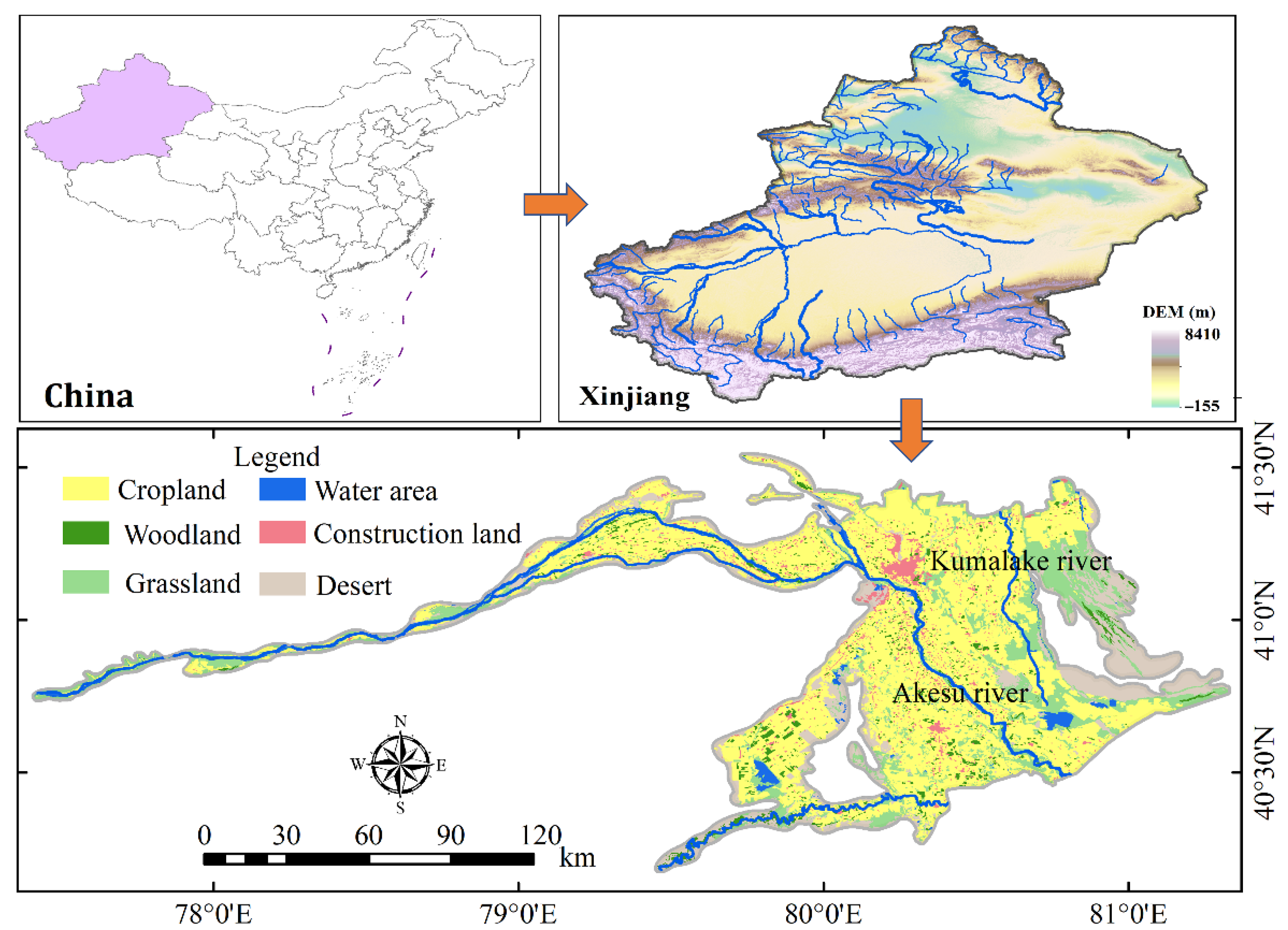
2. Overview of the Study Area

The subbasin of the Tarim River Basin is the Aksu River Basin. It originates near the base of the western portion of the middle Tianshan Mountains in the south. Study area is situated in northwest China (Figure 1, 77°25’~81°19’ E, 40°10’ ~ 41°33’ N) and encompasses around 1.1 × 10⁴ km² (Figure 1). The basin has a mild temperate arid climate with distinct continental climatic features, including aridity, high evaporation, and little precipitation. It is one of China’s and the world’s most environmentally sensitive regions. The basin terrain in the north is high, in the south is low, slopes from northwest to southeast, and is dominated by mountainous and flat regions of the two primary landscapes.

The Aksu basin is the largest irrigated oasis agricultural region in Xinjiang, a significant grain and fruit production center, and a significant cotton-producing region in China. With the adoption of China’s western development policy, agriculture and industry in the basin have seen significant growth, while urbanization and industrialization have grown steadily. The development has presented possibilities for the economic and social growth of the basin, as well as new concerns for the basin’s ecological protection: the groundwater level has been lowering, and significant habitats such as the Populus forest have been damaged progressively. Consequently, with the aid of high-resolution remote sensing data to achieve large-scale and high-precision ecological environment monitoring and driving research, it is possible to scientifically evaluate the ecological security of the basin, to coordinate the relationship between rapid economic development and ecological environment, and to promote the basin’s sustainable development.

3. Research Method

In this paper, a remote sensing ecological index (RSEI) model was developed using principal component analysis and remote sensing images from the GEE platform as the data source in order to investigate the spatial and temporal variation characteristics of ecological environment quality in Aksu watershed from 2000 to 2020. In addition, the Mann–Kendall trend test was employed to examine the trend of change in RSEI. Using the Pearson correlation coefficient and Moran’s I index, the combined RSEI indicators’ reliability and spatial rationality were evaluated. Using seven assessment indicators of greenness, humidity, dryness, heat, temperature, land use, and soil type as independent variables and RSEI grade as the dependent variable, a geographic probe was used to investigate the driving forces of geographical variability of RSEI in the watershed. To match the vegetation growing season, select the growing season (June–October) for the Rain, Vegetation Coverage, Groundwater reserves data to calculate the mean for use with correlation analysis.

3.1. Calculation Method Data Sources

In this research, the MODIS product set served as the data source, and MODIS data for the study region from 2000 to 2020 were imported online using the JavaScript API and the GEE platform. The necessary RSEI data were retrieved or estimated based on the atmospheric conditions (such as gas, aerosol, and Rayleigh scattering). The 500 m resolution (16-day composite) NDVI vegetation index was taken from the MOD13A1 V6 picture collection, while the time series LST images were extracted from the MOD11A2 product. The surface reflectivity data of MOD09A1 V6 products is utilized to determine the relative humidity and dryness components [27]. Data and sources used in the study are shown in

Table 1. Data and sources used by the Institute.

Ecological Indicators	Time Period	Time Resolution	Spatial Resolution	Data Source
RSEI	2000–2020	8 days/8 days/16 days	500 m/1000 m/500 m	MOD09A1/MOD11A2/MOD13A1
LUCC	2000–2020	—	30 m	Institute of Geography, Chinese Academy of Sciences (http://www.dsac.cn) accessed on 13 August 2022
TEM	2000–2020	1 month	1000 m	Monthly Mean Temperature Data of China (http://www.geodata.cn), accessed on 13 July 2022
ST	2008	—	10°	ISRIC report 2008/06 and GLADA report 2008/03
Rain	2000–2020	1 month	1000 m	Monthly precipitation data of China (http://www.geodata.cn), accessed on 13 July 2022
Vegetation Coverage	2000–2018	8 days	0.05°	GLASS_FVC_avhrr products (http://www.geodata.cn/) accessed on 13 May 2022
Groundwater reserves	2003–2020	1 month	0.25°	GRACELevel-2(RL06)/GLDAS
Construction’s GDP	2000–2020	per annum	—	Xinjiang Bureau of Statistics

.

Moreover, the 2000–2020 land use data utilized in this research were obtained from the Institute of Geography of the Chinese Academy of Sciences/Geographical Conditions Monitoring Cloud Platform (http://www.dac.cn, accessed on 13 August 2022), with a data spatial resolution of 30 m. The temperature and precipitation data are from the National Earth System Science Data Center (http://www.geodata.cn, accessed on 13 July 2022), with a data spatial resolution of 1000 m. The vegetation coverage data from 2000 to 2018 were obtained from the National Earth System Science Data Center’s GLASS FVC_avhrr product (http://www.geodata.cn, accessed on 13 May 2022). The data has a geographical resolution of 0.05 degrees and a temporal resolution of 8 days. ISRIC and GLADA 2008 global soil type data with a spatial resolution of 10° are used to generate soil type data. GRACELevel-2 (RL06)/GLDAS provides groundwater storage data from 2003 to 2020 with a geographical resolution of 0.25° and a time resolution of January. From the figures of the Xinjiang Bureau of Statistics, we may calculate the construction industry’s 2000–2020 GDP.

3.2. Analysis Method

1.

RSEI calculation technique

This research employed MOD09A1, MOD13A1, and MOD11A2 data from the GEE platform to determine the humidity, greenness, dryness, and heat index for each year. After normalizing each indicator’s data, the ecological index for remote sensing was produced using principal component analysis (PCA) [27,28], the RSEI calculation process is shown in Figure 2.

(1)

Greenness index

This study directly extracts the vegetation index (NDVI) of MOD13A to represent the greenness index.

(2)

Dryness index

In this study, the dryness index (NDBSI) is used to represent the dryness index, or the degree of surface “dryness”. In addition to bare property, development land must also be considered. The following is the formula:

$$\mathrm{NDBSI}=\frac{\mathrm{SI}+\mathrm{IBI}}{2}$$

(1)

$$\mathrm{SI}=\frac{\left[\left({\mathsf{\rho }}_{\mathrm{SWIR}1}+{\mathsf{\rho }}_{\mathrm{Red}}\right)-\left({\mathsf{\rho }}_{\mathrm{NIR}}+{\mathsf{\rho }}_{\mathrm{Blue}}\right)\right]}{\left[\left({\mathsf{\rho }}_{\mathrm{SWIR}1}+{\mathsf{\rho }}_{\mathrm{Red}}\right)+\left({\mathsf{\rho }}_{\mathrm{NIR}}+{\mathsf{\rho }}_{\mathrm{Blue}}\right)\right]}$$

(2)

SI is the index of bare soil; IBI is the building index, which is computed as follows:

$$\mathrm{IBI}=\frac{\{2{\mathsf{\rho }}_{\mathrm{SWIRI}}+\left({\mathsf{\rho }}_{\mathrm{SWIR}1}+{\mathsf{\rho }}_{\mathrm{NIR}}\right)-[\frac{{\mathsf{\rho }}_{\mathrm{NIR}}}{{\mathsf{\rho }}_{\mathrm{NIR}}+{\mathsf{\rho }}_{\mathrm{Red}}}+\frac{{\mathsf{\rho }}_{\mathrm{Green}}}{\left({\mathsf{\rho }}_{\mathrm{Green}}+{\mathsf{\rho }}_{\mathrm{SWIR}1}\right)}\}}{\{2{\mathsf{\rho }}_{\mathrm{SWIRI}}+\left({\mathsf{\rho }}_{\mathrm{SWIR}1}+{\mathsf{\rho }}_{\mathrm{NIR}}\right)+[\frac{{\mathsf{\rho }}_{\mathrm{NIR}}}{{\mathsf{\rho }}_{\mathrm{NIR}}+{\mathsf{\rho }}_{\mathrm{Red}}}+\frac{{\mathsf{\rho }}_{\mathrm{Green}}}{\left({\mathsf{\rho }}_{\mathrm{Green}}+{\mathsf{\rho }}_{\mathrm{SWIR}1}\right)}\}}$$

(3)

(3)

Wetness index

This study chooses the wetness index component (WET) to represent wetness. The wetness component is obtained by remote sensing the transformation of tasseled cap. The following is the formula:

$$\begin{gathered} \mathrm{WET} =0.2408{\mathsf{\rho }}_{\mathrm{Blue}}+0.3132{\mathsf{\rho }}_{\mathrm{Green}}+0.1147{\mathsf{\rho }}_{\mathrm{Red}}+ \\ 0.2489\mathsf{\rho }\_\mathrm{NIR}-0.6416\mathsf{\rho }\_\mathrm{SWIR}1-0.3122\mathsf{\rho }\_\mathrm{LWIR}-0.5087{\mathsf{\rho }}_{\mathrm{SWIR}2}) \end{gathered}$$

(4)

(4)

Heat index

In this work, the MOD11A2 surface temperature (LST$\_$Day 1 km) is used and the heat index is calculated.

LST = 0.02 (LST_Day_1 km) − 273.15

(5)

In summary, ${\mathsf{\rho }}_{\mathrm{NIR}}$ represents the reflectivity of the near-infrared band in all calculations, while ${\mathsf{\rho }}_{\mathrm{SWIR}1}$ and ${\mathsf{\rho }}_{\mathrm{SWIR}2}$ represent the reflectivity of the shortwave infrared bands 1 and 2, respectively. The values ${\mathsf{\rho }}_{\mathrm{Red}}$, ${\mathsf{\rho }}_{\mathrm{Blue}}$, and ${\mathsf{\rho }}_{\mathrm{Green}}$ represent the reflectance of the red band, blue band, and green band, respectively.

The normalization of the four computed indicators is as follows:

$${\mathrm{ND}}_{\mathrm{i}}=\left({\mathrm{D}}_{\mathrm{i}}-{\mathrm{D}}_{\min }\right)/\left({\mathrm{D}}_{\max }-{\mathrm{D}}_{\min }\right)$$

(6)

$N{D}_i$ is the result of index normalization; $D_i$ is the value of the i-th pixel; $D_{min}$ is the lowest value; and $D_{max}$ is the maximum value [29].

After standardizing the four indicators, the ENVI program [27] conducted principal component analysis, combining the four normalized indicator bands into a new picture. The baseline ecological index RSEI₀ was calculated by subtracting 1 from PC1 such that a big value would indicate a healthy ecosystem.

$${\mathrm{RSEI}}_0=1-\left\{ \mathrm{PC}1\left[\mathrm{f}\left( \mathrm{NDVI}, \mathrm{Wet}, \mathrm{LST}, \mathrm{NDSI}\right)\right]\right\}$$

(7)

${\mathrm{RSEI}}_0$ is the starting ecological index; $\mathrm{PC}1$ is the contribution value of the first main component; and NDVI, Wet, LST, and NDSI are the normalized values of humidity, greenness, dryness, and temperature, respectively.

Normalization of PC1 after positive and negative transposition yielded the remote sensing ecological index (RSEI):

$$\mathrm{RSEI}=\left({\mathrm{RSEI}}_0-{\mathrm{RSEI}}_{0\min }\right)/\left({\mathrm{RSEI}}_{0\max }-{\mathrm{RSEI}}_{0\min }\right)$$

(8)

RSEI is the remote sensing ecological index [30] in the formula, and its value is between 0 and 1. The better the ecological quality, the greater the RSEI value. RSEI_0min and RSEI_0max correspond to the least and maximum values of RSEI₀. This publication separates the RSEI index into four categories of habitat conditions based on the RSEI scenario in the study region and prior research findings [27]: low (RSEI 0.2), medium (0.2 RSEI 0.4), good (0.4 RSEI 0.6), and excellent (RSEI > 0.6).

2.

Average correlation

During the study period, the Pearson correlation coefficients between the five indicators (RSEI, WET, NDVI, NDSI, and LST) were computed, and the average correlation was determined [24] (S_p). The phrase is: the closer the S_p result is to 1, the more thorough the representation of the index. The expression is:

$${\mathrm{S}}_{\mathrm{p}}=\left(\left|{\mathrm{S}}_{\mathrm{q}}\left|+\right|{\mathrm{S}}_{\mathrm{r}}\left|+\cdots \right|{\mathrm{S}}_{\mathrm{s}}\right|\right)/\left(\mathrm{n}-1\right)$$

(9)

S_p is the average correlation degree, S_q, S_r, and S_s are the Pearson correlation coefficients between the indicators, and n is the number of indicators in the correlation analysis.

3.

Global Moran’s I

The Global Moran’s I tool (ArcGIS) is used to compute the z-score and p-value in order to determine the Moran’s I index value. Here, z-score closely resembles the standard deviation, whereas p denotes the likelihood. The distribution of Moran’s index value is [−1, 1]. Positive values show a positive connection between geographical entities, and the closer the value is to 1 the stronger the positive association. There is a negative connection between [−1, 0]; however, there is no correlation for the number 0.

4.

Mann–Kendall trend test

To investigate the trend of RSEI, the significance of the change is assessed and tested using the monotonic trend test technique of Mann–Kendall. Using a two-sided test to examine the data, when |Zc| is less than 1.96, the sample sequence exhibits a noticeable trend shift at the 0.05 significance level; when |Zc| is more than 2.58, the sample sequence’s trend changes considerably at the 0.01 significance level. A positive Zc represents an upward trend, whereas a negative Zc represents a downward trend [27].

5.

Geographic detector

Wang Jinfeng et al. [31] hypothesized that geodetectors are mostly used for the detection of geographical heterogeneity. In this work, the geographical heterogeneity of RSEI in the Aksu Basin was quantified using factor detection, interaction detection, and risk detection using geodetector [22,32]. Both human and natural causes influence the ecological environment quality of Aksu Basin. The seven evaluation indices of greenness, humidity, dryness, heat, temperature, land use, and soil type were used as independent variables, and the RSEI level was used as the dependent variable, in conjunction with the local dry and hot climate conditions and the effect of human activities on the ecological environment. The natural breakpoint approach was used to identify the independent variables, and a 2 × 2 km grid distribution sampling was constructed to exclude the aberrant points. Additionally, 2714 grid point sampling data were gathered and inputted into the geographic detector for computation.

(1)

The calculation formula for the factor detector is:

$$q=1-\frac{{{\displaystyle \sum }}_{\mathrm{h}=1}^{\mathrm{L}}{\mathrm{N}}_{\mathrm{h}}{\mathsf{\sigma } }_{\mathrm{h}}^2}{{\mathrm{N}\mathsf{\sigma } }^2}$$

(10)

In the formula, q is the influence of evaluation index X on Y, h = 1,2,..., L is the stratification of variable Y or factor X, N and Nh are the number of elements in the entire region and layer h, respectively, and ${\mathsf{\sigma } }_{\mathrm{h}}^2$ and σ² are the variances of the value of Y in layer h and the entire region, respectively [33]. The value of q is spread between 0 and 1; the bigger the value, the greater the effect, and vice versa.

(2)

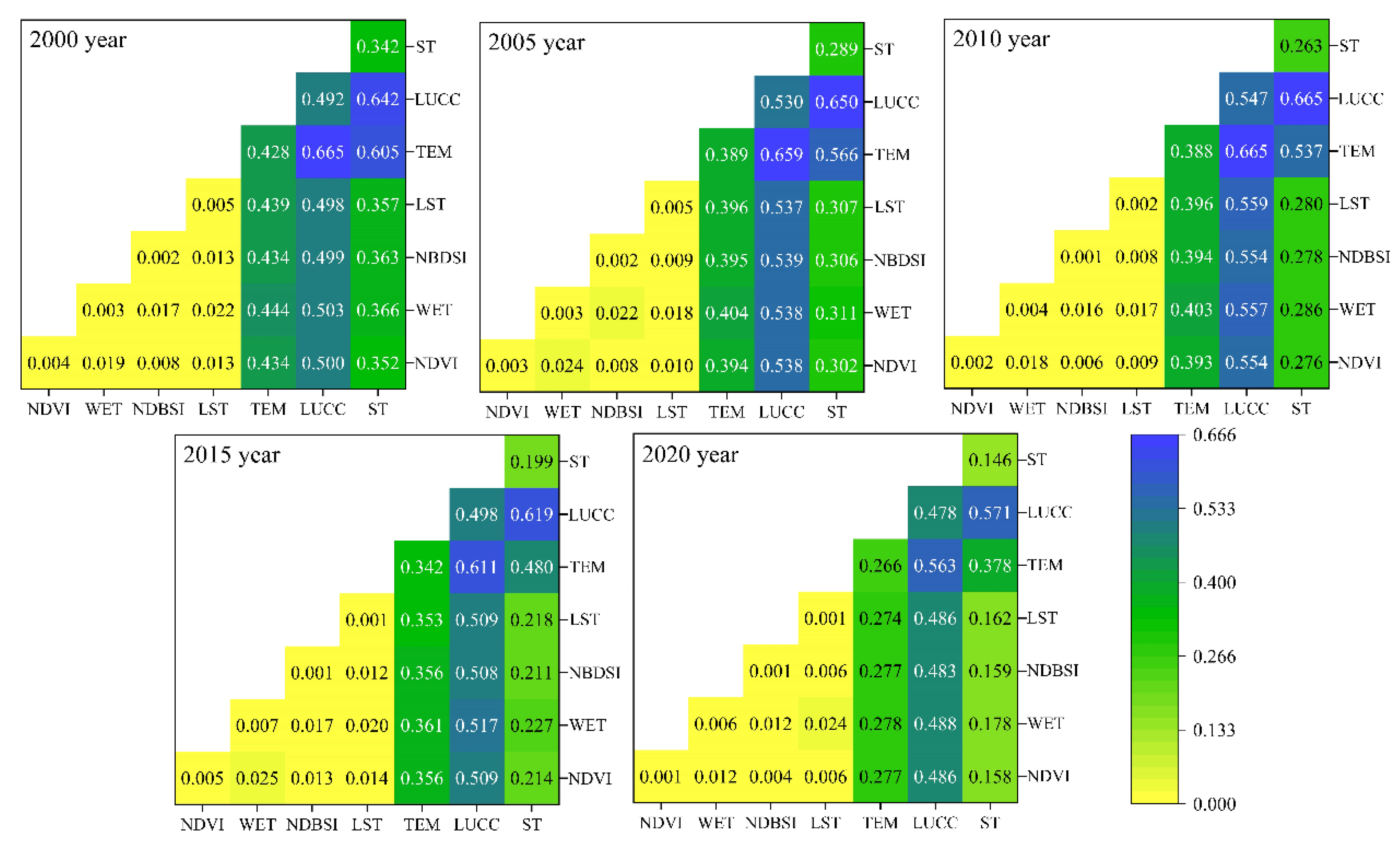
Interaction detector: Interaction detectors are primarily used to determine the interac tion between input index (X₁, X₂) and output index (Y) [28]. In this work, interaction detector is used to investigate the effect of multi-factor interaction on ecological environment quality. By comparing the respective q values [$q$ (X1), $q$ (X2)], interaction q values [$q$(X1 X2)], and the total of the q values [$q$(X1) + $q$ (X2)] of the output variable Y, [34] the interactions are classified into five groups (

Table 2. Interaction classification criteria.

Interaction Type	Judgment Criterion
Nonlinear weakening	$q$(X1∩X2) < Min[$q$(X1), $q$(X2)]
Single factor nonlinear weakening	Min[$q$(X1), q(X2)] < $q$(X1∩X2) < Max[$q$(X1), $q$(X2)]
wo-factor enhancement	$q$(X1∩X2) > Max[$q$(X1),$q$(X2)]
Mutually independent	$q$$($$\left($(X2)
Nonlinear Enhancement	$q$$($$\left($(X2)

).

4. Results

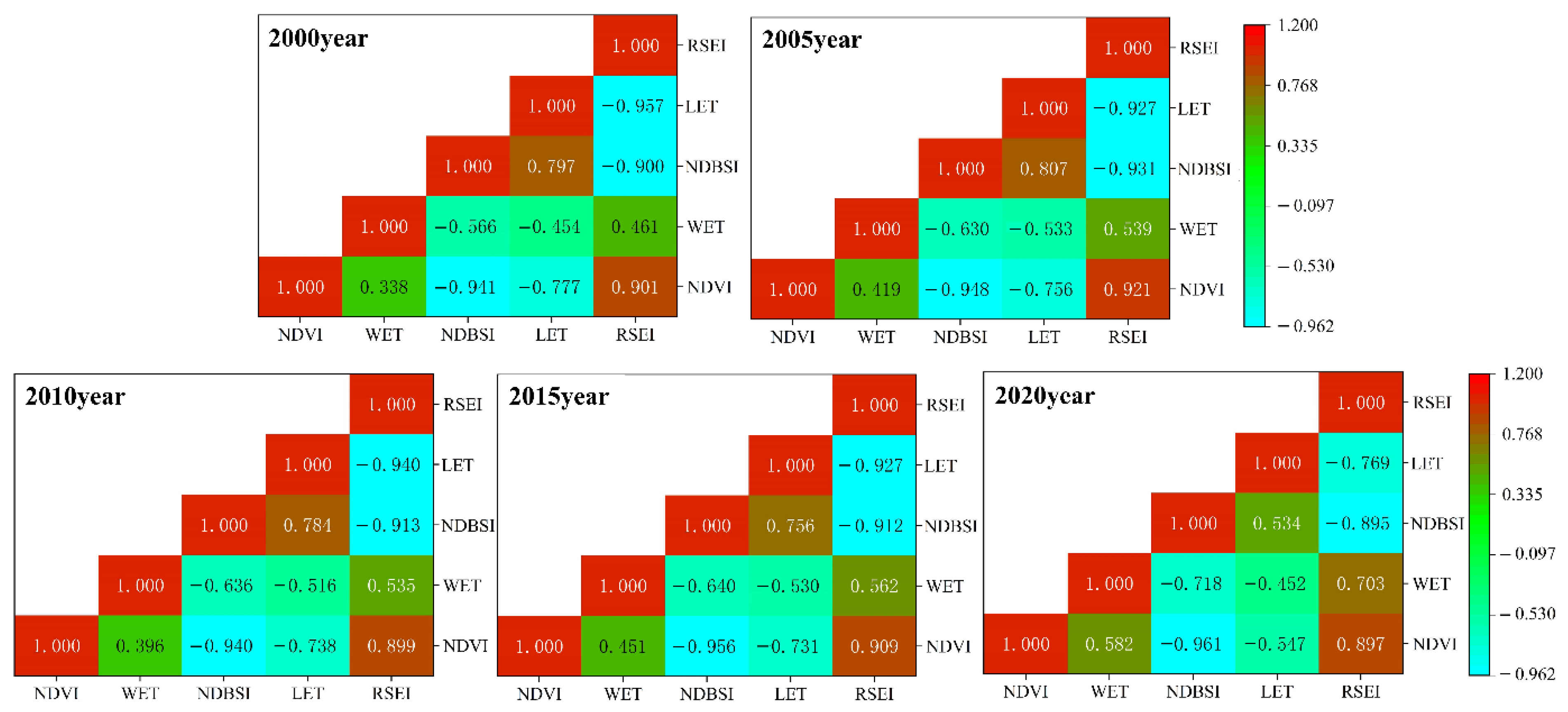
4.1. Advantages of RSEI

Correlation coefficient between RSEI and ecological variables as measured by Pearson (Figure 3). The results demonstrated that ecological variables and RSEI were important at the 1% level. RSEI was favorably connected with WET and NDVI and negatively correlated with NDBSI and LST, indicating that greenness and humidity had a large beneficial effect in the ecological environment, while dryness and heat played a substantial detrimental one (Figure 3). During the research period, the correlation between WET and RSEI rose, suggesting that its favorable impact on the natural environment increased. The average degree of association between each measure is as follows: RSEI > NDBSI > NDVI > LST > WET (

Table 3. Statistical chart of average correlation degree based on correlation coefficient.

Year	RSEI	NDVI	WET	NDBSI	LET
2000	0.805	0.739	0.455	0.801	0.746
2005	0.830	0.761	0.530	0.829	0.756
2010	0.822	0.743	0.521	0.818	0.745
2015	0.828	0.762	0.546	0.816	0.736
2020	0.816	0.747	0.614	0.777	0.576
Mean	0.820	0.750	0.533	0.808	0.712

). RSEI has a correlation coefficient that is 9.26%, 53.81%, 1.44%, and 15.22% more than NDVI, WET, NDSI, and LST, respectively. The multi-factor composite RSEI model is shown to be more practicable and applicable than any single index.

The findings of Global Moran I (Figure 4) indicate that the p values of the five-period data from 2000 to 2020 are all 0.000, which is statistically significant, and the z-score is very high (z-score > 281.28), with a 99% level of confidence. This analysis can thus confidently reject the null hypothesis that there is a substantial autocorrelation between the RSEI of each geographical unit, and the spatial distribution of the composite RSEI model is plausible.

In comparison to the five Global Moran’s I, the Moran’s I of every year throughout the research period was larger than 0.9118, indicating a substantial positive autocorrelation and spatial self-correlation. Among them, Moran’s I in 2000 was 0.9248, had a very high z-score (281,286) and a very low p-value (0.000) [35], and had the largest positive autocorrelation. Incorporating the average correlation degree with the findings of Global Moran’s I, the composite RSEI model is more practicable, adaptable, and spatially acceptable, and it has significant spatial autocorrelation.

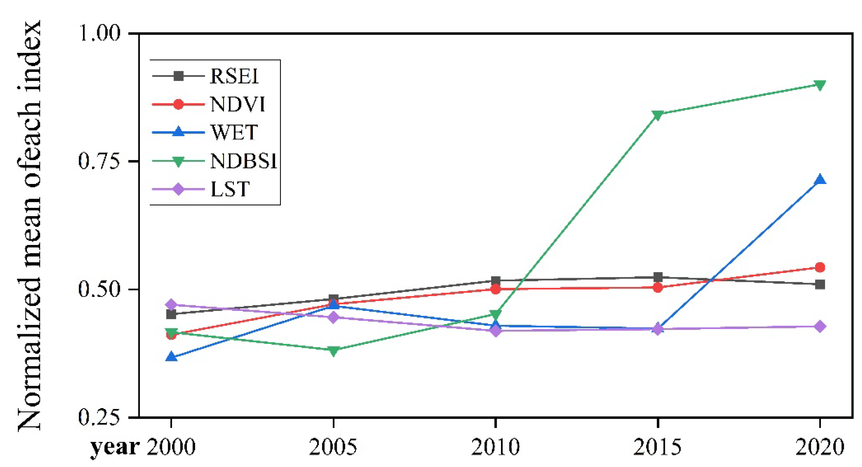
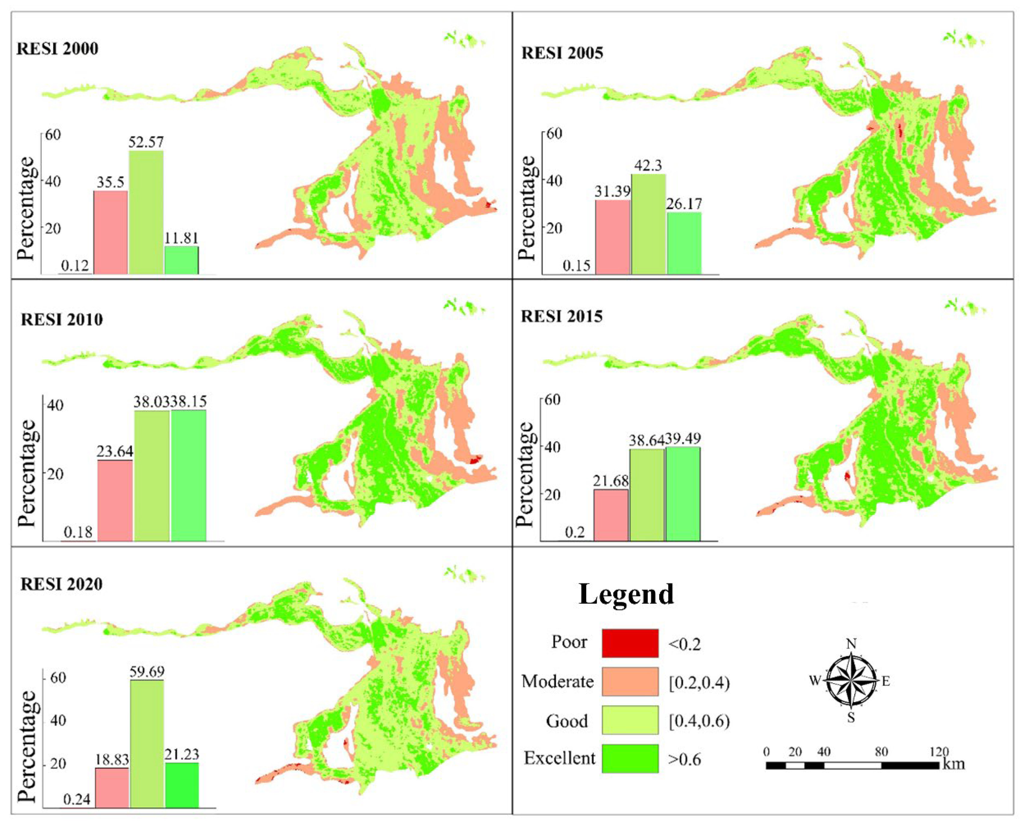
4.2. Temporal and Spatial Variation of Remote Sensing Ecological Index (RSEI)

Based on the temporal variations of each indicator and the mean value of the RSEI from 2000 to 2020 (Figure 5), the RSEI of the Aksu River Basin throughout the research period increased by 12.89%, from 0.4522 to 0.5105. In the last 21 years, the greenness, humidity, and dryness of the single index have grown by 31.95%, 94.278%, and 116.09%, respectively, while the temperature has declined by 9.022%. The increased trend of NDVI and WET is compatible with RSEI, which encourages the improvement of the natural environment. The declining trend of LST might also contribute to the rise of the regional RSEI index. The expansion of NDBSI impeded the environmental progress. The full research reveals that the indicators have contributed to the rise of the RSEI index and the improvement of the natural environment in the Aksu River Basin.

To more intuitively represent the ecological context and distribution, the RSEI values are categorized as bad, medium, good, and excellent. The ecological grades and proportions are tallied according to the RSEI values [0, 0.2], [0.2, 0.4], [0.4, 0.6], and [0.6, 1]. Figure 6 illustrates that the ecological environment quality level of the Aksu River Basin is mostly good and outstanding, with an area percentage of more than 64 percent, and the proportion of bad grade is the lowest (<0.25 percent).

Based on the regional distribution of the remote sensing ecological environment index (Figure 6), the Gobi, alluvial fan, and human settlements have the lowest environmental quality levels. The natural environment is degraded due to the effects of a dry and hot temperature and human building activity. The region around the Aksu basin, which is dominated by agriculture, has a higher quality level due to improved water conditions, increased plant covering, and an improved biological environment. Since the adoption of a series of ecological measures in 2000, such as ecological water conveyance, the change trend of good and outstanding grades has increased from 64.38 percent to 80.92 percent, and the ecological environment quality of the basin has improved.

According to Figure 7, the percentage of pixel area with a growing RSEI trend (Zc ≥ 0) in the Aksu River basin from 2000 to 2020 is 79.97%, which is much greater than the proportion of pixel area with a dropping RSEI trend (Zc > 2.58], which reaches up to 45.1%. The ecological quality of Aksu River Basin showed an improving trend [36]. The pixel area of substantial increasing trend [1.96 < Zc < 2.58) and non-significant rising trend [0 < Zc < 1.96) is 9.66% and 24.52%, respectively, whereas the pixel area of falling trend (Zc < 0) is 20.03%. A considerable drop (Zc < −1.96) barely reached 4.84 percent) The majority of regions with an increasing tendency in RSEI (Zc > 0) are located to the southeast of Aksu City, to the east and south of Wensu County, to the east of Keping County, to the southwest of Awati County, and to the northwest of Alar City from a spatial viewpoint. Flood irrigation of farmland, ecological water distribution, and other techniques to enhance regional water conditions, encourage the development of agricultural plants, and progressively improve ecological quality. The regions with a falling trend (Zc < 0) are mostly located in the southern portion of Wensu County, the northern portion of Aksu City, and the northern and northeastern portions of Awati County.

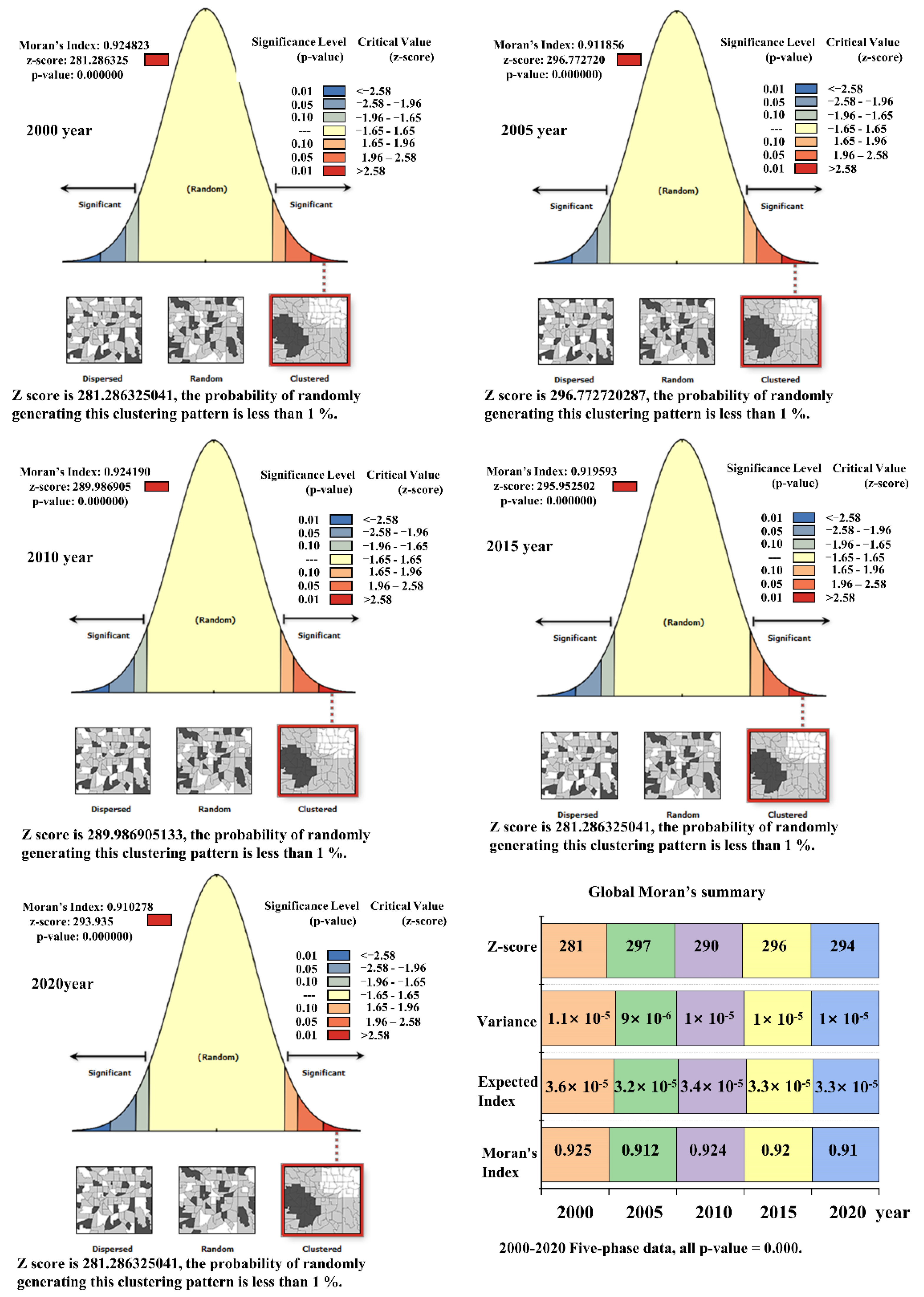
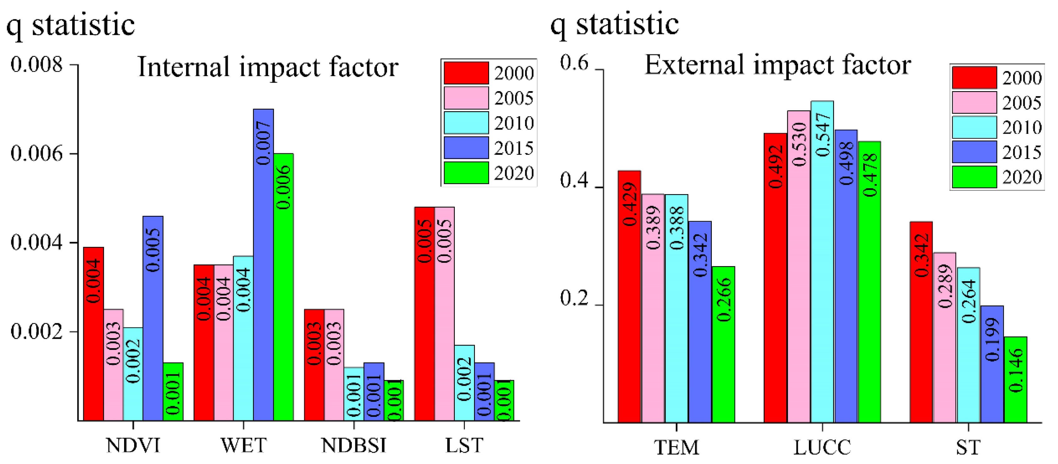
4.3. Spatial Heterogeneity Detection

Figure 8 displays that the explanatory power of the spatial differentiation characteristics of external factors was much greater than that of internal factors, indicating that the spatial heterogeneity of the ecological environment in the Aksu Basin was primarily driven by [36] external factors such as temperature (TEM) and land use (LUCC). The external explanatory power of the basin’s natural environment is enough (p = 0); however, the internal elements are lacking. In general, the explanatory power of land use indicators exceeds 45 percent, which is a significant factor influencing the change in the basin’s natural environment. Temperature and soil type are secondary variables with an explanatory power of more than 10%. The four internal driving elements of DVI, WET, NDBSI, and LST have less explanatory power for environmental quality. According to the time series, the effect of land use initially grew and subsequently reduced, but the temperature and soil type decreased gradually.

The findings of factor interaction (Figure 9) demonstrated that the contribution rate of interaction between any two variables to eco-environmental quality was more than that of a single component, and that both of them were two-factor enhancements. It demonstrates that the Akesu basin’s biological environment is not the product of a single element, but rather the interplay of several variables. From the viewpoint of external factors, the contribution of interaction between land use (LUCC) and other variables were larger than 0.478, suggesting that the largest effect of single factor test findings in the interaction with other factors to detect, its influence would be substantially amplified. The temperature (TEM) and soil type (ST) interaction forces with other indicators were more than 0.26 and 0.146, respectively. In general, exogenous variables (LUCC, TEM, and ST) have a substantial influence on the geographic variation of RSEI within the basin.

5. Discussion

1. 

The superiority of RSEI model

The RSEI composite score eliminates the influence of human weighing and takes into account the four primary environmental impact elements of green, wet, hot, and dry. Additionally, the RSEI composite index has both positive and negative components. RSEI is favorably connected with WET and NDVI, and negatively correlated with NDSI and LST, as shown by its spatial correlation coefficient (Figure 3). In contrast to a single index, the assessment findings are therefore objective and exhaustive.

In addition, the average degree of association based on Pearson’s correlation coefficient reveals (Table 3) that RSEI > NDBSI > NDVI > LST > WET. The average correlation degree of RSEI (0.820) is superior to that of single indicators, suggesting that RSEI is more effective and representative than single indicators. Five global Moran’s I indicate that RSEI’s Moran’s I is larger than 0.9118, indicating a positive autocorrelation and a substantial spatial autocorrelation. It demonstrates that the geographical distribution of the RSEI composite model is realistic. Nonetheless, we must recognize the limits of analyzing RSEI only by correlation analysis of other satellite derivatives. If ground observation data can be used in future study, the RSEI assessment impact will be enhanced.

2. 

Double effects of human factors

(1) Ecological measures to promote ecological quality. From the timeline (Figure 10) it can be seen that during the implementation of ecological protection measures between 2000 and 2020, the groundwater storage in the Aksu Basin increased, the vegetation coverage increased annually, and the ecological environment quality of Aksu was significantly enhanced. RSEI simple linear regression (Figure 10 reveals that the slope of the yearly average RSEI change is larger than zero, suggesting that the ecological environment quality is rising. From 2000 to 2020, the average RSEI climbed by 12.89 percent. Overall good and exceptional ratings grew from 64.38 percent to 80.92 percent, and the quality of the ecological environment was enhanced. Moreover, the enhancement of plant cover plays a crucial role in the restoration and management of ecological environments [36]; thus, we must pay close attention to the conservation of watershed vegetation.

From 2000 to 2020, 79.97% of pixel area in the Aksu River Basin exhibited an increasing trend (Zc > 0) for RSEI. From a geographical standpoint (Figure 7), the southeast portion of Aksu City, the eastern and southern portions of Wensu County, the eastern portion of Keping County, the southwestern portion of Awati County, and the northwest portion of Alar City have greatly improved. This region is mostly agricultural. Due to the execution of a series of ecological measures in the year 2000, the water-holding capacity of agricultural soil was increased, the development of farmland vegetation was encouraged, and the ecological quality was steadily upgraded.

(2) Urban expansion inhibits ecological quality improvement. Due to the delicate biological environment of the oasis basin, coordinating economic growth and environmental conservation remains a formidable problem [37]. The primary causes of environmental degradation [38,39] are the negative consequences of human activities on ecosystems. Significant degradation of ecological environment quality is spatially localized mostly in the urbanization growth zone (Figure 7). This outcome is inextricable from economic building operations. Increase in building land is more likely to result in high temperatures and dry soil, NDBSI grew dramatically, and the urban heat island effect is evident, leading in the degradation of the original regional ecological environment. After 2005, the construction industry’s GDP in the Aksu River Basin has been very consistent with the NDBSI trend (Figure 11). In 2012, Aksu started implementing urban system planning in conjunction with faster urbanization, increasing building activity, and a considerable growth in NDBSI. In 2015 and 2020, the NDBSI will exceed 0.75, increasing the pressure on RSEI progress. In addition, the growth of the city absorbs the cultivated land and forest land around the city, which diminishes the vegetation cover in the urban area and hinders the improvement of the quality of the ecological environment.

3. 

Spatial heterogeneity driving factors

Through the identification of geographical detector components, it is possible to determine that both human and natural causes contribute to RSEI. The findings indicate that temperature and land use are the primary drivers of geographical variation in RSEI. Land use is the key element influencing the spatial variation of the basin’s biological environment, and the synergistic impact of its interaction with other variables is considerably amplified. The findings of single factor and interaction between components indicate that land use has the most explanatory power; hence, land use is the most influential factor. Changes in land use are mostly influenced by urbanization. Construction land replaces agricultural land, woodland, and grassland, resulting in decreased plant covering, exposed surface, and severe dryness [26,40]. Additional examination of the link between temperature, precipitation, and RSEI (Figure 12). Except for the years 2007–2011, the RSEI had a definite upward trend, with slight fluctuations. The precipitation reduced first, then surged, and then decreased again. Beginning in 2012, the temperature soared and then plummeted, and the oscillation was evident. The significant coefficients (

Table 4. Chart of correlation statistics of temperature, rainfall and RSEI.

Spearman Correlation Coefficient		Rain	Tem
RSEI	correlation coefficient	0.38	0.376
	Significance (two-tailed)	0.871	0.093

) between the three variables are more than 0.05, and the correlation is not significant. Therefore, temperature and precipitation are not the most influential elements on RSEI. According to the detector’s findings, land use is the key factor influencing the regional variation of the basin’s biological environment, and its influence on RSEI is much greater than that of precipitation and temperature. Additionally, groundwater storage and RSEI exhibited a consistent upward tendency (Figure 9).

Therefore, in regions with dense human activity, sensible landscape pattern design may further enhance the ecological quality of the regional environment. Expanding building land may expand green space, such as parks and green belts, to guarantee that metropolitan areas have sufficient plant covering and soil retention. In addition, research on the connection between groundwater storage change land use, and vegetation covering, as well as NDBSI, should be bolstered in the future to support the growth of regional green economies.

6. Conclusions

Based on the GEE platform, MODIS image data, Pearson correlation coefficient, Moran’s I index, and geographic detector, the RSEI comprehensive index’s reliability was determined, the ecological environment status and its change trend of Aksu River Basin from 2000 to 2020 were analyzed, and the external driving factors of spatial heterogeneity of RSEI were discussed.

(1)

Compared to the single index, the composite RSEI model has a higher average correlation, and the RSEI model’s Moran’s I index is more than 0.9118, suggesting that the spatial positive correlation is stronger. Therefore, the composite RSEI model has more practicability, dependability, and geographical plausibility.

(2)

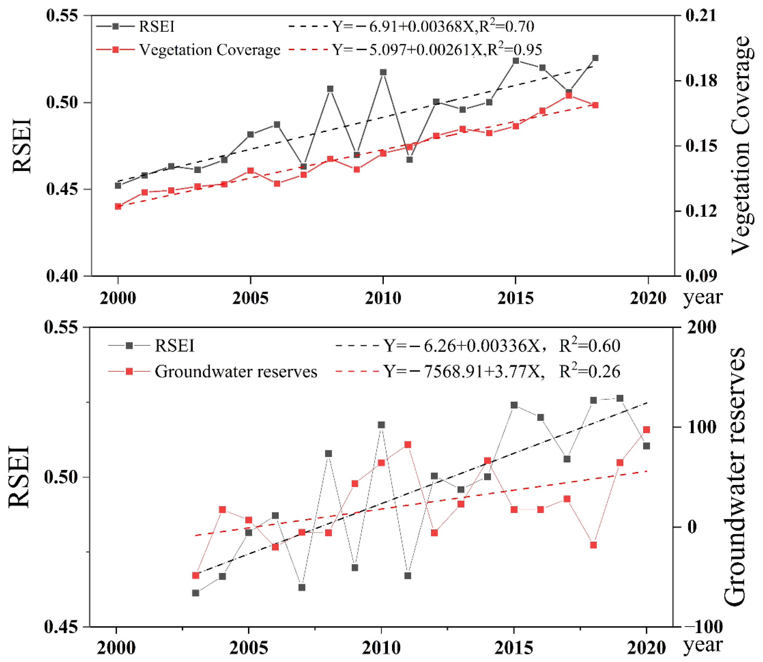
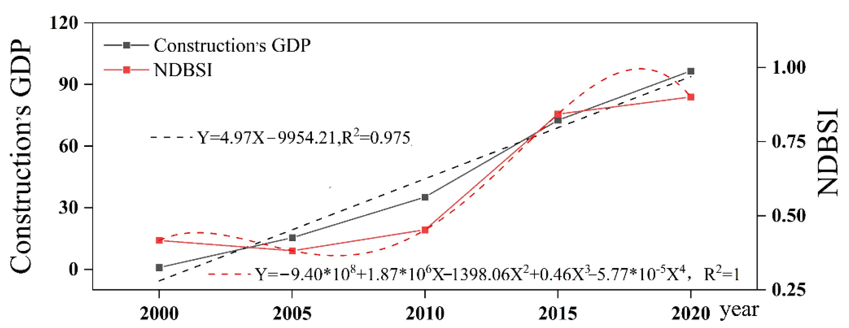
The natural environment quality of Aksu basin is impacted in two ways by human influences. (1) The adoption of ecological protection measures to boost the Aksu groundwater storage and increased plant covering, and to enhance the ecological environment’s quality. Following the adoption of ecological protection measures, the average RSEI rose by 12.89%, the ecological quality of the farmland-based region improved considerably, and the quality of the ecological environment was enhanced. (2) Urban growth hinders the improvement of ecological quality. As urbanization accelerates, NDBSI rises dramatically, exerting pressure on RSEI enhancements. In addition, the growth of cities and towns, the occupancy of arable land and forest land, and the decline of urban area vegetation cover diminish the quality of the natural environment.

(3)

Both human and environmental causes contribute to the regional variability of RSEI in Aksu Basin. The geographical heterogeneity is mostly caused by temperature and land use, with land use being the most important driver. Strengthening research on the connection between groundwater storage change, land use, vegetation cover, and NDBSI may facilitate the growth of regional green economies.

References

- Gao, P.; Kasimu, A.; Zhao, Y.; Lin, B.; Chai, J.; Ruzi, T.; Zhao, H. Evaluation of the Temporal and Spatial Changes of Ecological Quality in the Hami Oasis Based on RSEI. Sustainability 2020, 12, 7716. [Google Scholar] [CrossRef]
- Zuo, L.; Zhang, Z.; Zhao, X.; Wang, X.; Wu, W.; Yi, L.; Liu, F. Multitemporal analysis of cropland transition in a climate-sensitive area: A case study of the arid and semiarid region of northwest China. Reg. Environ. Change 2014, 14, 75–89. [Google Scholar] [CrossRef]
- Fan, Q.D.; Ding, S.Y. Landscape pattern changes at a county scale: A case study in Fengqiu, Henan Province, China from 1990 to 2013. Catena 2016, 137, 152–160. [Google Scholar] [CrossRef]
- Li, A.; Wang, A.; Liang, S.; Zhou, W. Eco-environmental vulnerability evaluation in mountainous region using remote sensing and GIS—A case study in the upper reaches of Minjiang River, China. Ecol. Model. 2006, 192, 175–187. [Google Scholar] [CrossRef]
- Das, S.; Pradhan, B.; Shit, P.; Alamri, A. Assessment of Wetland Ecosystem Health Using the Pressure-State-Response (PSR) Model: A Case Study of Mursidabad District of West Bengal (India). Sustainability 2020, 12, 5932. [Google Scholar] [CrossRef]
- Li, N. Analysis of Water Resources Carrying Capacity in Planning Environmental Impact Assessment. Urban Environ. Urban Ecol. 2012, 25, 22–26. [Google Scholar]
- Qing, Q.P.; Wang, Y. Dynamic evaluation and study on difference of eco-environmental quality in the provinces. China Environ. Sci. 2019, 39, 750–756. [Google Scholar]
- An, M.; Li, W.; Wu, H.; An, H.; Huang, J. Evolution and Influencing Factors of the Spatial-Temporal Pattern of Ecological Environment Quality in the Three Gorges Reservoir Area. Sustainability 2018, 10, 3854. Available online: https://www.mdpi.com/355808 (accessed on 25 November 2022).
- Strobel, C.J.; Buffum, H.W.; Benyi, S.J.; Paul, J.F. Environmental Monotoring and Assessment Program: Current Status of Virginian Province (U.S.) Estuaries. Environ. Monit. Assess. 1999, 56, 1–25. [Google Scholar] [CrossRef]
- Ramírez-Cuesta, J.; Minacapilli, M.; Motisi, A.; Consoli, S.; Intrigliolo, D.; Vanella, D. Characterization of the main land processes occurring in Europe (2000–2018) through a MODIS NDVI seasonal parameter-based procedure. Sci. Total Environ. 2021, 799, 149346. [Google Scholar] [CrossRef]
- Moghimi, M.M.; Zarei, A.R.; Mahmoudi, M.R. Seasonal drought forecasting in arid regions, using different time series models and RDI index. J. Water Clim. Change 2020, 11, 633–654. [Google Scholar] [CrossRef]
- Xu, P.W.; Zhao, D. Ecological environmental quality assessent of Hangzhou urban area based on RS and GIS. Chin. J. Appl. Ecol. 2006, 17, 1034–1038. [Google Scholar]
- Xu, H.Q. A remote sensing index for assessment of regional ecological changes. China Environ. Sci. 2013, 33, 889–897. [Google Scholar]
- Wu, S.; Gao, X.; Lei, J.; Zhou, N.; Guo, Z.; Shang, B. Ecological environment quality evaluation of the Sahel region in Africa based on remote sensing ecological index. J. Arid. Land 2022, 14, 14–33. [Google Scholar] [CrossRef]
- Lin, Y.; Nan, X.; Hu, Z.; Li, X.; Wang, F. Fractional vegetation cover change and its evaluation of ecological security in the typical vulnerable ecological region of Northwest China: Helan Mountains in Ningxia. J. Ecol. Rural. Environ. 2022, 38, 599–608. [Google Scholar]
- Ariken, M.; Zhang, F.; Liu, K.; Fang, C.; Kung, H.-T. Coupling coordination analysis of urbanization and eco-environment in Yanqi Basin based on multi-source remote sensing data. Ecol. Indic. 2020, 114, 106331. [Google Scholar] [CrossRef]
- Yang, Z.; Tian, J.; Li, W.; Su, W.; Guo, R.; Liu, W. Spatio-temporal pattern and evolution trend of ecological environment quality in the 13 Yellow River Basin. Acta Ecol. Sin. 2021, 41, 7627–7636. [Google Scholar]
- Chun, L.; Hui, L.; Yue, Q.L. Ecological change assessment based on remote sensing index-taking Changning City as an example. Remote Sens. Land Resour. 2014, 26, 145–150. [Google Scholar]
- Wang, S.; Zhang, X.; Zhu, T.; Yang, W.; Zhao, J. Remote sensing evaluation of eco-environmental quality in Changbaishan Nature Reserve. Adv. Geogr. 2016, 35, 1269–1278. [Google Scholar]
- Cheng, P.G.; Tong, C.Z.; Chen, X.Y.; Nie, Y.J. Urban Ecological Environment Monitoring and Evaluation Based on Remote Sensing Ecological Index. In Proceedings of the International Conference on Intelligent Earth Observing and Applications 2015, Guilin, China, 23 October 2015. [Google Scholar]
- Liu, Z.; Xu, H.; Li, L.; Tang, F.; Lin, Z. Urban Ecological Change of Hangzhou Based on Remote Sensing Ecological Index. J. Appl. Basic Eng. Sci. 2015, 23, 728–739. [Google Scholar]
- Lin, S.; Xu, H.; Lin, Z. Dynamic changes and ecological analysis of bare soil in Changting soil erosion area. Fujian For. Sci. Technol. 2015, 42, 7–12+39. [Google Scholar]
- Liao, W.H.; Jiang, W.G. Evaluation of the Spatiotemporal Variations in the Eco-environmental Quality in China Based on the Remote Sensing Ecological Index. Remote Sens. 2020, 12, 2462. [Google Scholar] [CrossRef]
- Ning, L.; Wang, J.Y.; Fen, Q. The improvement of ecological environment index model RSEI. Arab. J. Geosci. 2020, 13, 403. [Google Scholar] [CrossRef]
- Xiong, J.; Li, W.; Zhang, H.; Cheng, W.; Ye, C.; Zhao, Y. Selected Environmental Assessment Model and Spatial Analysis Method to Explain Correlations in Environmental and Socio-Economic Data with Possible Application for Explaining the State of the Ecosystem. Sustainability 2019, 11, 4781. [Google Scholar] [CrossRef] [Green Version]
- Zhang, K.; Feng, R.; Zhang, Z.; Deng, C.; Zhang, H.; Liu, K. Exploring the Driving Factors of Remote Sensing Ecological Index Changes from the Perspective of Geospatial Differentiation: A Case Study of the Weihe River Basin, China. Int. J. Environ. Res. Public Health 2022, 19, 10930. [Google Scholar] [CrossRef]
- Jiao, A.; Wang, W.; Deng, X.; Ling, H.; Yan, J.; Chen, F. Effect evaluation of ecological water conveyance in Tarim River Basin, China. Front. Environ. Sci. 2022, 10, 1718. [Google Scholar] [CrossRef]
- Shi, H.; Shi, T.; Liu, Q.; Wang, Z. Ecological Vulnerability of Tourism Scenic Spots: Based on Remote Sensing Ecological Index. Pol. J. Environ. Stud. 2021, 30, 3231–3248. [Google Scholar] [CrossRef]
- Guo, B.; Fang, Y.; Jin, X. Monitoring the effects of land consolidation on the ecological environmental quality based on remote sensing: A case study of Chaohu Lake Basin, China. Land Use Policy 2020, 95, 104569. [Google Scholar] [CrossRef]
- Li, P. Research on Ecoenvironmental Quality Evaluation System Based on Big Data Analysis. Comput. Intell. Neurosci. 2022, 2022, 5191223. [Google Scholar] [CrossRef]
- Kumar, P.; Sharma, M.C.; Saini, R.; Singh, G.K. Climatic variability at Gangtok and Tadong weather observatories in Sikkim, India, during 1961–2017. Sci. Rep. 2020, 10, 15177. [Google Scholar] [CrossRef]
- Geng, J.; Yu, K.; Xie, Z.; Zhao, G.; Ai, J.; Yang, L.; Yang, H.; Liu, J. Analysis of Spatiotemporal Variation and Drivers of Ecological Quality in Fuzhou Based on RSEI. Remote Sens. 2022, 14, 4900. [Google Scholar] [CrossRef]
- Fu, J.; Zhang, Q.; Wang, P.; Zhang, L.; Tian, Y.; Li, X. Spatio-Temporal Changes in Ecosystem Service Value and Its Coordinated Development with Economy: A Case Study in Hainan Province, China. Remote Sens. 2022, 14, 970. [Google Scholar] [CrossRef]
- He, Y.; Wang, W.; Chen, Y.; Yan, H. Assessing spatio-temporal patterns and driving force of ecosystem service value in the main urban area of Guangzhou. Sci. Rep. 2021, 11, 3027. [Google Scholar] [CrossRef] [PubMed]
- Boori, M.S.; Choudhary, K.; Paringer, R.; Kupriyanov, A. Spatiotemporal ecological vulnerability analysis with statistical correlation based on satellite remote sensing in Samara, Russia. J. Environ. Manag. 2021, 285, 112138. [Google Scholar] [CrossRef] [PubMed]
- Xiong, Y.; Xu, W.; Lu, N.; Huang, S.; Wu, C.; Wang, L.; Dai, F.; Kou, W. Assessment of spatial temporal changes of ecological environment quality based on RSEI and GEE: A case study in Erhai Lake Basin, Yunnan province, China. Ecol. Indic. 2021, 125, 107518. [Google Scholar] [CrossRef]
- Liu, R.; Dong, X.; Zhang, P.; Zhang, Y.; Wang, X.; Gao, Y. Study on the Sustainable Development of an Arid Basin Based on the Coupling Process of Ecosystem Health and Human Wellbeing Under Land Use Change-A Case Study in the Manas River Basin, Xinjiang, China. Sustainability 2020, 12, 1201. [Google Scholar] [CrossRef] [Green Version]
- Runting, R.K.; Bryan, B.A.; Dee, L.E.; Maseyk, F.J.; Mandle, L.; Hamel, P.; Wilson, K.A.; Yetka, K.; Possingham, H.P.; Rhodes, J.R. Incorporating climate change into ecosystem service assessments and decisions: A review. Glob. Change Biol. 2017, 23, 28–41. [Google Scholar] [CrossRef] [Green Version]
- Wang, H.; Liu, G.; Li, Z.; Zhang, L.; Wang, Z. Processes and driving forces for changing vegetation ecosystem services: Insights from the Shaanxi Province of China. Ecol. Indic. 2020, 112, 106105. [Google Scholar] [CrossRef]
- Yan, N.; Zeyue, M.; Profeng, Z.; Lei, Y.; Jing, Y. Research on soil moisture inversion and monitoring in the Aksu River basin. J. Ecol. 2019, 39, 5138–5148. [Google Scholar]