Application of Soil Moisture Data Assimilation in Flood Forecasting of Xun River in Hanjiang River Basin

Abstract

Accurate projection of floods is of great significance to safeguard economic and social development as well as people’s life and property. The development of hydrological models can improve the level of flood projection, however, the numerous uncertainties in the models limit the projection accuracy. By adding observations to correct the operation of prediction models, the accuracy can be improved to some extent. In this paper, taking the Xun River, of the Hanjiang River Basin in China, as the research object, combined with the soil moisture satellite data obtained by the soil moisture active and passive satellite (SMAP), the ensemble Kalman filter (EnKF) algorithm was used to assimilate the upper soil water content (WU) of the Xinanjiang model. In addition, based on the simultaneous assimilation of state variables and parameters, two improved assimilation schemes were proposed here, namely, the augmented ensemble Kalman filter (AEnKF) scheme and the dual ensemble Kalman filter (DEnKF) scheme. The results showed that compared with the WU assimilation scheme, the simultaneous assimilation of parameters and WU improved the prediction ability of the Xinanjiang model to a greater extent. The two improved schemes had similar effects on flood prediction accuracy, and improved the overall Nash–Sutcliffe efficiency coefficient (NSE) from 0.725 for non-assimilated, and 0.758 for assimilated WU, to 0.781. Among them, AEnKF and DEnKF schemes, respectively, improved the NSE by 10.1% and 11% at maximum. This study demonstrated that the application of data assimilation for the Xun River effectively improved the flood forecast accuracy of the Xinanjiang model, which will provide a reference basis and technical support for future flood prevention and mitigation and flood projection in this basin.

1. Introduction

The frequent occurrence of extreme hydrological events creates flood disasters causing more and more damage to people’s lives [1], which has become an important issue affecting economic and social development. The complex and diverse topography and continental monsoon climate cause most of the rainfall in China to be concentrated within a period of time, which to a certain extent also exacerbates the frequency and extent of floods [2]. In July 2021, the city of Zhengzhou, China, was hit by a once-in-a-millennium extraordinarily heavy rainfall [3], with more than 200 mm of precipitation in just one hour from 16:00 to 17:00 on the 20th; and about 620 mm of precipitation in three days, from the 17th to the 20th. According to the “7.20 rainstorm disaster investigation report” released by the State Council Disaster Investigation Group in China, a total of 150 counties (cities and districts) in Henan Province, with a population of 14.78 million people, were affected, with direct economic losses amounting to RMB 120.6 billion. This shows that flood prevention and mitigation is of great significance to ensure people’s safety, social stability and economic development. Based on the available hydro-meteorological data, flood projection can qualitatively and quantitatively analyze and predict possible future floods [4]. It is regarded as a very important non-engineering initiative to provide a reference for flood control and scheduling decisions. Timely and accurate flood projection is useful for making scientific flood control decisions to avoid risks, but the question of how to further improve flood projection accuracy above the current level is still a research focus for hydrologists.

Hydrological models can simulate a real system and predict changes in relevant variables [5]. With the development of hydrology, more and more practical hydrological models have been put forward, such as the Stanford model [6], API model [7], Xinanjiang model [8], SWAT model, etc. These models can be classified into three categories: empirical models, conceptual models, and physically based models [5]. Of these, empirical models lack the relevant physical mechanism; they only obtain information from the existing data, resulting in a large randomness of prediction results. Physically based models are constructed based on the principles of physical processes. They require a large number of data, and the non-linear calculation process is complicated, causing their application to be limited. Compared with the above two types of models, conceptual models are both physical and empirical, and can describe the water cycle process in the basin with simplified equations. The conceptual models have good applicability to most basins in China because of their low requirements regarding the number of parameters and accuracy of the modeling data, and simple structure. Actually, the widely used Xinanjiang model is a conceptual model type. Considering that the Xun River in the Hanjiang River Basin belongs to the subtropical semi-humid climate zone, which meets the storage and flow production mechanism of the Xinanjiang model, this paper has chosen it as the appropriate flood prediction model.

Hydrological model parameters can quantify the characteristics of vegetation, soil, and stream channels in a watershed [9]. In general, it is not easy to obtain their true values due to the numerous uncertainties in the models, but it is necessary to estimate the parameters in a practical study that takes into account the spatial and temporal heterogeneity of the watershed and the scale of the parameters. The parameter values affect the accuracy of the models. The mainstream method used by hydrologists to determine the parameters is to continuously tune them to obtain simulation results that are highly consistent with past observations, which is called parameter calibration [10]. It is essentially a robust optimization problem under the model uncertainties from a mathematical point of view [11]. Compared with manual calibration methods with certain subjectivity and experience, automatic calibration has been favored by many scholars because of its efficiency and objectivity. However, due to the randomness and uncontrollability of hydrological processes, predicting future floods by using parameters obtained from historical hydrological data calibration will lead to inestimable errors. Therefore, it is necessary to correct the hydrological state variables and model parameters by means of relevant technical methods. At present, the correction algorithms have been greatly enriched, such as feedback simulation technology, error autoregression algorithm (AR) [12], recursive least squares algorithm (RLS) [13,14], Kalman filter (KF) [15,16] and dynamic system response curve algorithm (DSRC) [17], etc. Generally, AR and RLS are more commonly used to estimate the model parameter, while KF is used to estimate the state.

The development of remote sensing observation technology has broadened the access to data and enriched the existing sources of observation data, which makes data assimilation more applicable to hydrological projection. Data assimilation takes into account both forecast and observational information, helps to quantify and reduce uncertainty in hydrological applications, and is effective in water level forecasting and/or flood forecasting [18]. The assimilation methods currently used in hydrology are divided into two categories according to the optimization path: one is the variational assimilation for global fitting, and the other is the sequential assimilation for real-time optimization [19]. Variational assimilation transforms the data assimilation process into a solution of extreme values by constructing a cost function to represent the difference between the analyzed and true values of the variables. After meeting the dynamic constraints, the state variable value that minimizes the difference between the observed and predicted values is taken as the optimal analysis value. However, the adjoint model established by variational assimilation requires continuous differentiability of the state variables, and the nonlinearity of the hydrological model makes it difficult to satisfy this, thus, limiting its application. Based on the error estimation theory, sequential assimilation updates the forecast in time sequence by adding new observations at each time step, generates the forecast background at the next moment, advances forward by time, and finally obtains the optimal estimation of parameters or state variables for the whole period. KF is the basic form of sequential assimilation, which was proposed by R.E. Kalman in 1960 [20]. It has the advantages of simplicity, small dependence on initial values, and good convergence, but it can only have unbiased optimal estimation if the system is linear and the noise is Gaussian white noise [21]. For nonlinear systems, some processing of KF is required.

Based on this, Evensen used the idea of ensemble projection in Kalman filtering and proposed the ensemble Kalman filter (EnKF) algorithm, which solved the shortcomings of the traditional KF when applied to a nonlinear system [22]. EnKF adds Gaussian white noise disturbances to model state variables and observation data, calculates Kalman gain and generates analysis ensemble at that time. Assuming that the mean value of analysis is the truth, the errors of the members of the analysis ensemble are calculated, and the error covariance of the analysis can be obtained. The mean value of the analysis and the error covariance matrix at that moment are applied to initialize the background in the next moment, so that the simulation is more consistent with the real probability distribution of the state variables. Reichle et al. [23] applied EnKF to the retrieval problem of soil moisture distributions and investigated the effect of ensemble size and non-Gaussian forecast errors on estimation accuracy, and the results showed that EnKF was a flexible and robust data assimilation option that could give satisfactory estimates. Reichle et al. [24] assessed the performance of the extended Kalman filter (EKF) and EnKF for soil moisture estimation, and the results indicated that EnKF was a promising approach for soil moisture initialization problems. Zhang et al. [25] investigated the ability to retrieve the true soil moisture profile by assimilating near-surface soil moisture into a soil moisture model with an EnKF assimilation scheme. Shen et al. [26] analyzed the basic theory and steps for data assimilation by using EnKF with an example based on numerical modeling, and drew the conclusion that EnKF can be used in groundwater level forecasting and pre-warning. Li et al. [27] applied a coupling model of support vector machines (SVM) and EnKF (SVM + EnKF) for rainfall–runoff simulation, and found that this model could substantially improve the accuracy of flood prediction compared with SVM. KF with state and parameter updating is the so-called adaptive Kalman filter (AKF). Additionally, there is the corresponding adaptive EnKF, e.g., [28], which can accelerate the speed of convergence and significantly improve the identification accuracy and search efficiency.

In this paper, the EnKF algorithm was applied to the Xinanjiang model to construct the EnKF data assimilation model, taking the Xun River of the Hanjiang River Basin as the study area. Combined with the measured data, WU and sensitive parameters (i.e., soil storage capacity curve index (B), and basin average free water storage capacity (SM)) of the model were assimilated and updated. The improvement of flood projection accuracy after assimilation was analyzed to assess the practicality of the data assimilation for flood projection for the Xun River, with a view to providing a reference basis and technical support for future flood prevention and mitigation, and flood projection. The paper is organized as follows: Section 2 introduces an overview of Xun River and the data, Section 3 describes the methods, Section 4 provides the results, and Section 5 is a summary.

2. Study Area and Data

2.1. Study Area

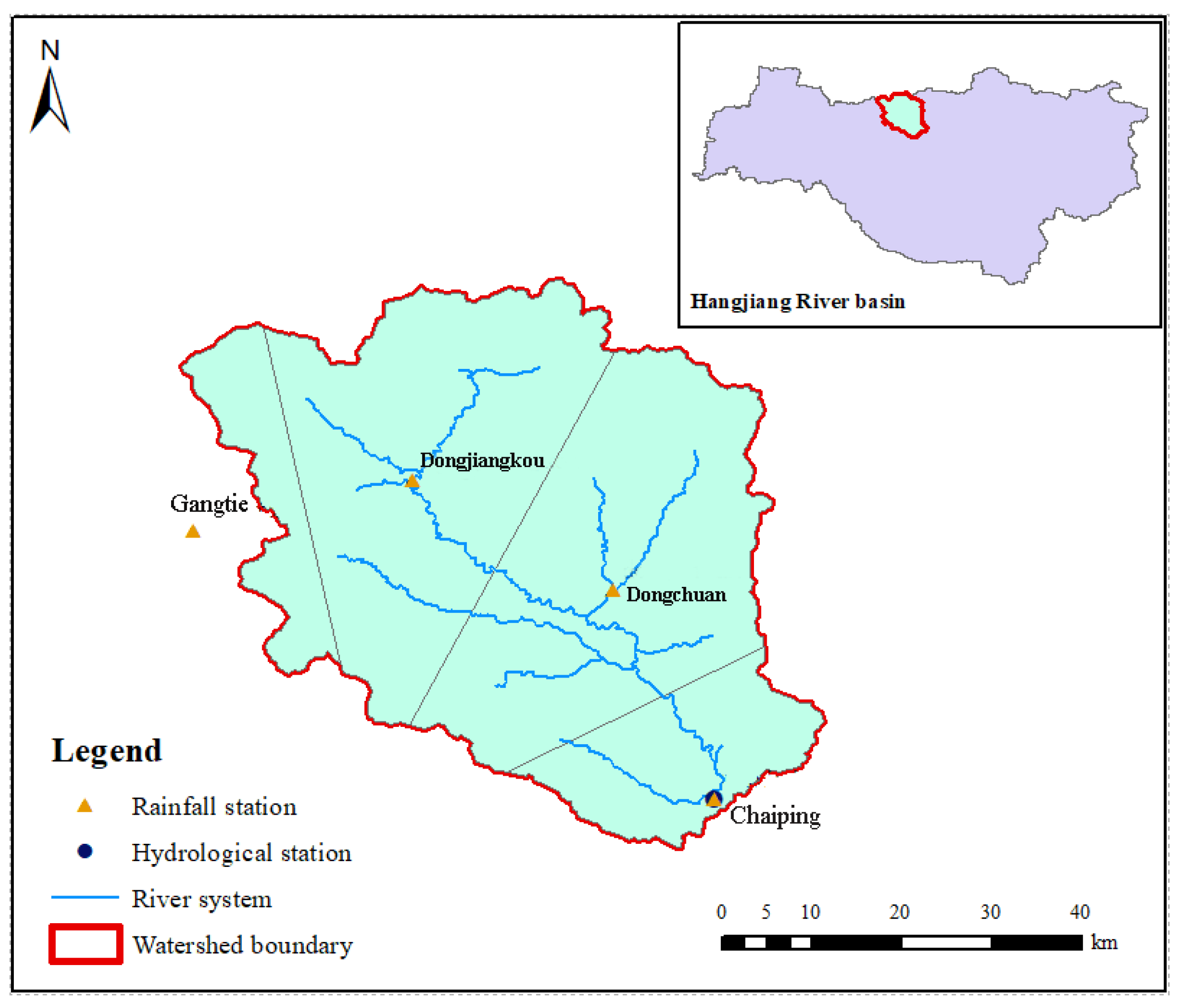
The Xun River originates from Ningshan County, Shaanxi Province, and is a first-class tributary of the Hanjiang River, with a length of 218 km. The upper reaches of the Xun River are located above Chaiping Station, with a length of 117 km and a watershed area of 2364 km². Abundant rainfall causes frequent floods in this area, which is characterized by a large peak volume (2690 m³/s). Therefore, accurate flood projection is necessary to maintain the safety of downstream power stations and people’s lives.

In this paper, the flood projection study was carried out for the watershed above Chaiping Station, the specific location of which is shown in Figure 1. The measured discharge of Chaiping Station in 1999–2021 was used for the flow data, in hourly units. Based on the rainfall observation data of four local major rainfall stations, the mean rainfall in the area for the corresponding period was calculated using Tyson polygon. For the surface evaporation observation E₀, due to the lack of actual measurement data, this study assumed 0.1 mm uniformly with reference to the adjacent watershed.

2.2. Data

2.2.1. Precipitation and Discharge Data

In this study, the measured runoff data from 1999 to 2021 at Chaiping Station in the upper reaches of Xun River were used. Rainfall data were selected from four rainfall stations in this area, namely, Gangtie, Dongjiangkou, Dongchuan and Chaiping. The Tyson polygon method was applied to determine the mean rainfall in this basin for the corresponding period, and the locations and weights of each rainfall station are shown in

Table 1. Location of each rainfall station and Tyson polygon weights.

Rainfall Stations	Gangtie Station	Dongjiangkou Station	Dongchuan Station	Chaiping Station
Location (east longitude/°)	108.42	108.64	108.84	108.94
Location (northern latitude/°)	33.60	33.65	33.54	33.33
Weights	0.0865	0.3889	0.3903	0.1343

. The 27 floods with better rainfall–flow relationships were selected based on the above information for subsequent analysis and research.

2.2.2. Soil Moisture Data

Soil moisture is one of the key variables characterizing the earth’s energy flow and hydrological cycle, which not only reflects evaporation, infiltration and runoff in hydrological models, but also has an important impact on flood prediction accuracy [29]. Currently, soil moisture data can be obtained by three main means, including traditional monitoring, model simulation and remote sensing observation. Among them, traditional monitoring methods rely on the establishment of meteorological stations in the field. Such data are generally of high accuracy, but the cost of manpower and material resources is large and not easily accessible to the public. The spatial heterogeneity of soil vegetation also limits the data obtained by this means for large watershed studies. Based on the principle of water balance, real-time soil moisture data can also be simulated by models, but it is still difficult to obtain accurate data in the modeling process and parameter setting. Remote sensing observation can monitor the earth’s soil moisture with the help of remote sensing satellites, which has the advantages of wide coverage, high accessibility, real time and convenience. Active microwave remote sensing and passive microwave remote sensing together constitute the current soil moisture data observed by satellites. The best performance in soil moisture observation is currently recognized as L-band, because it reflects higher sensitivity to the observed variables, compared with other bands.

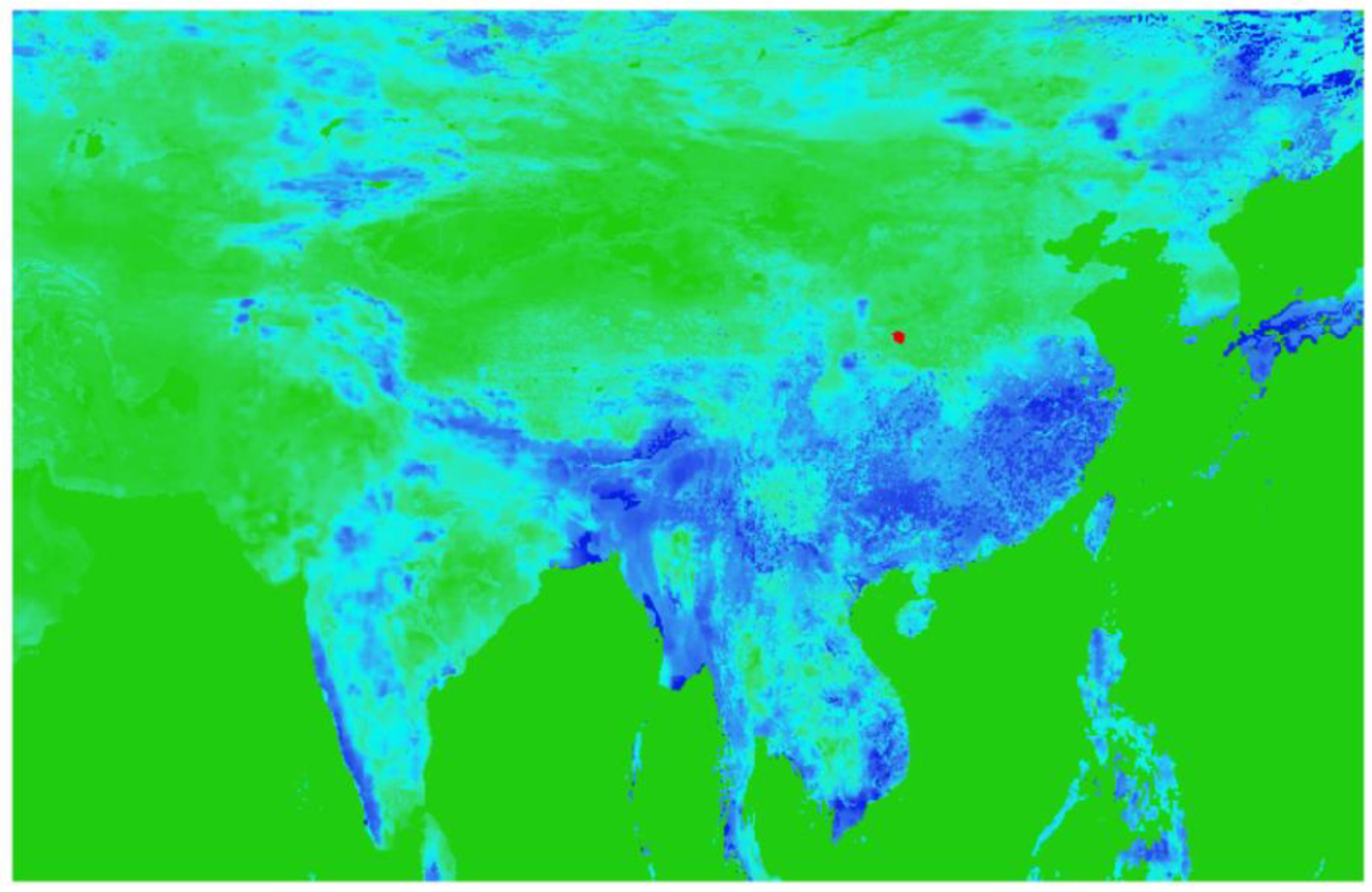
SMAP is an L-band satellite that can be used to observe soil moisture, launched by the National Aeronautics and Space Administration (NASA) in 2015 [30]. It has a combination of active and passive microwave sensors. Although the SMAP active radar is no longer available, its radiometer still provides highly accurate observations that can acquire surface 5 cm soil moisture data at spatial resolutions of 3 km, 10 km, and 40 km, and temporal resolutions of 1 to 3 days [31]. As the latest soil moisture monitoring satellite in orbit, the global soil moisture information provided by SMAP will make an important contribution to hydrometeorological studies and flood and drought prediction. The soil moisture data used in this paper were from the SMAP L4 product, which provides global 3-hour 9-km surface 5 cm soil moisture based on EASE-Grid 2.0. The global soil moisture data downloaded from the SMAP official website (Figure 2) were imported into ArcGIS for batch cropping to generate the corresponding raster data for the watershed above Chaiping (Figure 3), and the average soil moisture values of the watershed at each time were extracted as the data used for this assimilation.

The soil moisture observation data provided by SMAP represent the volumetric water content $\theta$ (cm³/cm³), and their characteristic values corresponding to the eight floods that will be assimilated are shown in

Table 2. Characteristic values of water content (cm³/cm³) corresponding to floods for assimilation.

	Volumetric Water Content	Maximum Value	Minimum Value	Average Value
Flood Number
1 (No. 20170927)		0.272	0.392	0.309
2 (No. 20171004)		0.304	0.361	0.322
3 (No. 20180704)		0.223	0.349	0.266
4 (No. 20190628)		0.149	0.329	0.196
5 (No. 20190807)		0.151	0.329	0.222
6 (No. 20190915)		0.210	0.357	0.297
7 (No. 20200819)		0.229	0.352	0.291
8 (No. 20210424)		0.213	0.372	0.272

. Since the subsequent state variables to be assimilated include WU of the Xinanjiang model, these data should be converted into watershed surface water depth ${\mathrm{D}}_{\mathrm{w}}$ (mm) in advance when used, as shown in Equation (1). In addition, the soil moisture data observed by SMAP, which had a temporal resolution of 3 h, was interpolated into a 1-hour form in this study to correspond to the rainfall–runoff data.

$${\mathrm{D}}_{\mathrm{w}}=h\times \theta \times 10$$

(1)

where h is the soil thickness observed by SMAP, taken as 5 cm; due to the unit conversion involved (cm converted to mm), it is also multiplied by 10.

3. Methodology

3.1. Xinanjiang Rainfall–Runoff Model

Zhao [32] proposed the Xinanjiang model after years of research and practical work experience, which was proved to achieve good results in flood simulation in most humid and sub-humid areas in China. Initially, the model divided the runoff into two parts, i.e., surface runoff and underground runoff. It did not take into account the subsurface runoff, which caused a high degree of nonlinear variation in the confluence process, and the flood simulation differed greatly from the actual situation. Subsequently, many domestic and foreign research results on production and confluence were referred, and a three-source model was formed by adding the subsurface flow [32]. Based on the good simulation effect of the Xinanjiang model for most areas in China, and the fact that Xun River in Hanjiang River Basin belongs to the subtropical semi-humid climate zone, which satisfies the mechanism of flood storage and production of the model, the Xinanjiang model was chosen as the flood projection model in this paper.

Due to the spatial and temporal heterogeneity of the rainfall in an actual basin, the Xinanjiang model uses a scattered structure to determine the basin outlet runoff, which mainly involves four steps: evapotranspiration calculation, runoff generation calculation, water source division, and confluence calculation. The calculation of runoff generation in the second step is particularly critical and has a significant impact on the accuracy of flood simulation. The runoff yield can be calculated according to the principle of full flow, i.e., when precipitation causes the soil water content of a watershed to meet its storage capacity, the difference between the storage capacity and soil moisture value at the beginning of rainfall is considered as the rainfall loss. At the same time, the uneven distribution of soil water shortage is solved through the basin water storage capacity area distribution curve, and the total runoff volume calculated is used for flood simulation [33]. The Xinanjiang model takes rainfall P and surface evaporation EM as inputs, and basin outlet section flow Q and actual evapotranspiration E as outputs [8].

At the beginning of rainfall, the amount of soil water content in the vadose zone will influence the process of rainfall forming runoff. Under the same rainfall conditions, a larger soil water content will produce more runoff volume. In the Xinanjiang model, the soil water content of the watershed is generally based on the evaporation, runoff and rainfall process in the early period, and can be derived from the water balance principle using the following recursive formula:

$$W_{t+1}=W_t+P_t-E_t-R_t$$

(2)

where $W_t$ is the soil water content at the initial moment at time t, measured in mm; $P_t$ is the rainfall at time t, measured in mm; $E_t$ is the evapotranspiration at time t, in mm; and $R_t$ is the runoff produced at time t, measured in mm. A constraint needs to be added in the calculation, namely, $0\le W\le W_m$, and $W_m$, which is the upper limit of soil water content in the basin, also known as the basin storage capacity.

3.2. SCE-UA Method

In principle, Xinanjiang model parameters should be determined by actual measurements or experiments according to their physical significance, but in practice, many parameters exist in the absence of observations or due to unsatisfactory observations. Many methods of parameter calibration have been developed. The general process is as follows: firstly, assume a set of initial parameters to drive the model simulation, compare the simulation with the measured data to further optimize the parameters, and gradually determine the parameter values that are closest to the actual situation. Finally, the unreasonable values should also be corrected by combining their physical meanings. Among them, the shuffled complex evolution (SCE-UA) algorithm developed by Duan et al. [34] is considered as a classic algorithm in this field because of its mature development, high efficiency in processing the non-smooth, insensitive and non-convex conditions of the reflection surface of the objective function, and its ability to ignore the influence of local minima.

The SCE-UA algorithm can consider both deterministic search and stochastic search, treating globalized search as a process of natural biological evolution. The algorithm constitutes a competitive complex evolutionary algorithm (CCE) by linking the complex search approach with the theory of competitive evolution of natural organisms. In this paper, the Xinanjiang model of Xun River in the basin above Chaiping was constructed based on the available hydrological data, and 27 representative floods were selected for the study. In view of the relatively mature development of the SCE-UA algorithm, its fast convergence speed and high operational efficiency, this paper adopted it to optimize the parameters of the Xinanjiang model with NSE as the objective function. The first 19 floods (1999–2013) were used for parameter calibration, and the last 8 floods (2017–2021) were applied for parameter verification. The parameter values, objective function, and calibration results of SCE-UA used in this paper are described as follows.

(1)

SCE-UA algorithm parameters

The first step in SCE-UA is to determine the number of complex forms, p. Zhang and Jiang [35] studied the influence of different p values on model parameter calibration when data are ideal. The results showed that, when the value of p is 1 or 2, the parameter truth value basically cannot be searched. When the value of p is increased (4 and 10 examples), the true values of most parameters can be searched. In general, when the data are in good condition, p ≥ 4 can basically meet the needs of optimization parameters. The more complex the shapes, the better the applicability to higher-order nonlinear scenarios. The parameter settings of SCE-UA in this study are shown in

Table 3. Parameter values in SCE-UA.

Parameter	n	m	q	p	s	α	β	k	P
Value	15	31	16	4	124	1	31	5	0.01%

.

In this table, n is the number of parameters; m is the number of complex vertices; q is the number of subcomplex vertices; p is the number of complex forms; s is the population size; α is the number of children generated by the parent; β is the number of generations generated by the parent; k is the number of cycles to stop the iteration; and P is the critical precision to stop the iteration.

(2)

Objective function

In this paper, NSE was chosen as the objective function. When NSE is closer to 1, it indicates the better simulation effect of the Xinanjiang model. The NSE calculation formula is as follows:

$$NSE=1-\frac{{\sum }_{t=1}^T{\left(Q_o^t-Q_m^t\right)}^2}{{\sum }_{t=1}^T(Q_o^t-{\overline{Q_o)}}^2}$$

(3)

where $Q_o^t$ is the measured runoff at time t; $Q_m^t$ is the simulated runoff at time t; and $\overline{Q_o}$ is the average of the observed runoff in this flood.

(3)

Parameter calibration results

The SCE-UA was used to optimize the parameters of the Xinanjiang model in the Xun River watershed above Chaiping, where the first 19 floods (1999–2013) were used for parameter calibration and the last 8 floods (2017–2021) were used for parameter validation and data assimilation. The parameter calibration ranges and final values are shown in

Table 4. SCE-UA algorithm parameter calibration range and values.

Parameter	K	UM	LM	DM	C	IM	B	SM
Upper limit	1.1	30	100	50	0.2	0.05	0.6	100
Lower limit	0.1	10	50	20	0.1	0.01	0.1	30
Value	0.38	20	73.30	48.61	0.18	0.04	0.5	70.6
Parameter	EX	KI	KG	CS	CI	CG	L
Upper limit	1.5	0.6	0.6	0.99	0.99	1	10
Lower limit	1	0.1	0.1	0.70	0.70	0.98	0.1
Value	1.24	0.25	0.5	0.92	0.90	0.998	4.92

.

(3)

Evaluation Indicators

Common indicators for evaluating a flood simulation include the relative error of flood peak ($Q_{re}$), peak time difference (ΔT), and NSE. NSE is given in Equation (3), and the remaining two indicators are as follows:

$$Q_{re}=\frac{Q_{m,max}-Q_{o,max}}{Q_{o,max}}\times 100\%$$

(4)

$$\Delta T=\left|T_m-T_o\right|$$

(5)

where $Q_{o,max}$ and $Q_{m,max}$ are the measured and simulated flood, respectively; and $T_o$ and $T_m$ are the measured and simulated peak occurrence times, respectively.

3.3. Ensemble Kalman Filter

KF is only suitable for linear systems. For nonlinear systems, some processing of KF is required. To improve the traditional KF algorithm, Evensen [22] used the idea of ensemble projection and proposed EnKF. The main idea is that after considering the model’s characteristics and the error distribution of the background and observation, a set of Gaussian white noise perturbations are added to the model state variables and observation data, respectively. The background and observation after the addition of the perturbations will enter the analysis step and generate the analysis ensemble at that moment. The statistical samples of the analysis errors are determined by the differences among the members of this ensemble, from which the error covariance of the analysis fields is estimated. This ensemble of analysis values is used to determine the initial state of the model at the next moment, to calculate the prediction ensemble of the next model run, and estimate the covariance of the prediction error according to the differences among the members of the ensemble.

The EnKF algorithm uses the Monte Carlo method to determine the prediction error covariance of state variables, and makes the calculation of the error covariance less difficult by ensemble. The advantage of this method is not only its lightweight computation, but also its usability in nonlinear systems. Due to its simplicity and efficiency, it is widely used in hydrology. The algorithm consists of two steps: prediction step (time update) and the analysis step (observation update). The prediction step is the update of the state variable in time dimension, predicting the value by the previous value. The analysis step is to add observation data to the prediction model and obtain the analysis value of state variables based on the update. The EnKF algorithm is as follows [36]:

(1)

Initialize background: given the background ensemble of EnKF $X_0=(X_{0,1}^a, X_{0,2}^a , \dots X_{0,n}^a$), the set number is n, and the state variable $X_{0,i}^a$ obeys the Gaussian distribution with mean $X_0^a$ and covariance $P_0^a$;

(2)

Add the state variable ensemble at time t to the prediction model, and calculate the next moment state variables $X_{t+1,i}^f$ and the prediction error covariance $P_{t+1}^f$.

$$X_{t+1,i}^f=M\left(X_{t,i}^a,{\alpha }_{t+1},{\beta }_{t+1}\right)+W_i$$

(6)

$$P_{t+1}^f=\frac{1}{n-1}{\displaystyle \sum }_{i=1}^n\left(X_{t+1,i}^f-\overline{X_{t+1}^f}\right){\left(X_{t+1,i}^f-\overline{X_{t+1}^f}\right)}^T$$

(7)

where $X_{t+z,i}^f$ is the i-th value in the state variable predicted ensemble at time t + 1; $\overline{X_{t+1}^f}$ is the average of the state variable predicted ensemble at time t + 1; $X_{t,i}^a$ is the i-th value in the analysis ensemble at time t; M(*) is the prediction model, which refers to the Xinanjiang model in this paper; $a_{t+1}^{}$ and ${\beta }_{t+1}$ correspond to the driving data and parameters of the model at time t + 1; and $W_i$ is the prediction error, which is assumed to be Gaussian white noise with mean 0 and variance Q;

(3)

Calculate the gain matrix $K_{t+1}$ at t + 1.

$$K_{t+1}=P_{t+1}^f{H}^T{\left(H{P}_{t+1}^f{H}^T+R\right)}^{-1}$$

(8)

$$P_{t+1}^f{H}^T=\frac{1}{n-1}{\displaystyle \sum }_{i=1}^n\left(X_{t+1,i}^f-\overline{X_{t+1}^f}\right)[H(X_{t+1,i}^f-H{\left(\overline{X_{t+1}^f}\right)]}^T$$

(9)

$$H{P}_{t+1}^f{H}^T=\frac{1}{n-1}{\displaystyle \sum }_{i=1}^n\left[H\left(X_{t+1,i}^f\right)-H\left(\overline{X_{t+1)}^f}\right)\right]{\left[H\left(X_{t+1,i}^f\right)-H\left(\overline{X_{t+1)}^f}\right)\right]}^T$$

(10)

where H(*) is the observation operator, which reflects the link between the predicted and observed values of state variables—a linear observation operator was used in this paper; and R is the observation error covariance;

(4)

Combine the predicted ensemble and observation at t + 1, and calculate the analysis ensemble $X_{t+1,i}^a$ and the analysis error covariance $P_{t+1}^a$ at this moment.

$$X_{t+1}^a,i=X_{t+1,i}^f+K_{t+1}\left(Z_{t+1}-H\left(X_{t+1,i}^f\right)+u_i\right)$$

(11)

$$P_{t+1}^a=\frac{1}{n-1}{\displaystyle \sum }_{i=1}^n\left(X_{t+1,i}^a-\overline{X_{t+1}^a}\right){\left(X_{t+1,i}^a-\overline{X_{t+1}^a}\right)}^T$$

(12)

where $X_{t+1,i}^a$ and $X_{t+1,i}^a$ are the i-th value in the predicted and analyzed ensembles of state variables at t + 1, respectively; $\overline{X_{t+1}^a}$ is the average of the state variables analyzed ensemble at t + 1; $Z_{t+1}$ is the observation corresponding to t + 1; H($X_{t+1,i}^f$) is the projection of state variables on the observation space; $u_i$ is the perturbation added to the observation, obeying a Gaussian distribution with mean 0 and variance R;

(5)

After the prediction update step, the cycle moves to the next moment.

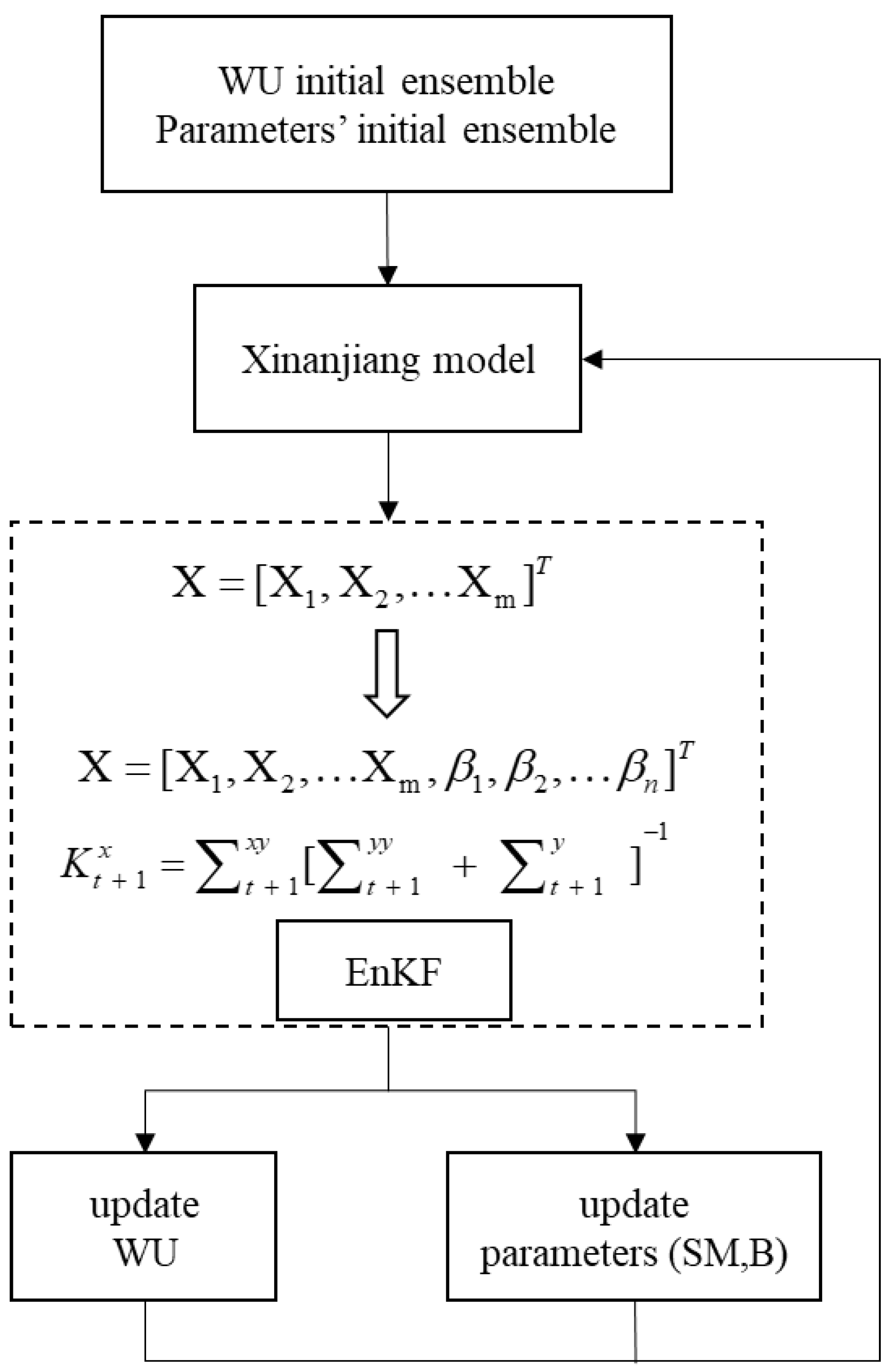
3.4. Augmented Ensemble Kalman Filter

The augmented ensemble Kalman filter (AEnKF) also treats the model parameters as special state variables, and combines the assimilated parameters and other state variables to form a multidimensional vector [37]. When there are observations, the parameters and state variables will be updated simultaneously to obtain the optimal estimate at that moment. In other words, parameters are added to $X={\left[X_1,X_2,\dots X_m\right]}^T$ to make it $X={\left[X_1,X_2,\dots X_m, {\beta }_1,{\beta }_3,\dots ,{\beta }_n\right]}^T$. m and n are the number of state variables X and model parameters β, respectively. The observation operator in this algorithm also needs to be adjusted to adapt to the vector dimension after adding the parameters. The subsequent filter process is the same as EnKF, where the ensemble of parameters and state variables is continuously updated during the assimilation process.

In this section, the original single-state variable WU was represented as a multi-state variable $X={\left[\mathrm{WU},B,SME\right]}^T$ after adding the parameters. B as the soil storage capacity curve index. The observed data were SMAP remote sensing soil moisture data, and the corresponding operator was $H={\left[1,0,0\right]}^T$. Generally, the value of observation error variance is 5% to 10% of the observed value, while the initial error variance tends to be higher due to the initial conditions are uncertain [38]. Thus, the observation error variance was set as 1, which was about 7% of the observed value, and the initial error variance was empirically set as 5, which was large enough to account for their uncertainties. The mean value of the WU initial ensemble was taken as the observed soil moisture at the initial moment to generate the background. For parameters B and SM, the mean values of the initial background ensemble were taken as the calibration value of SCE-UA, and the variances were taken as 0.12 and 102, i.e., $B~N(0.5,{0.1}^2)$ and $SM~N(70,{10}^2)$, respectively. During the model operation, WU and parameters B and SM of the Xinanjiang model were updated as a continuous forward filter. For comparison with the scheme of assimilating WU, other settings remained unchanged and the number of ensemble samples was still 200. The flow of the AEnKF algorithm is shown in Figure 4.

3.5. Dual Ensemble Kalman Filter

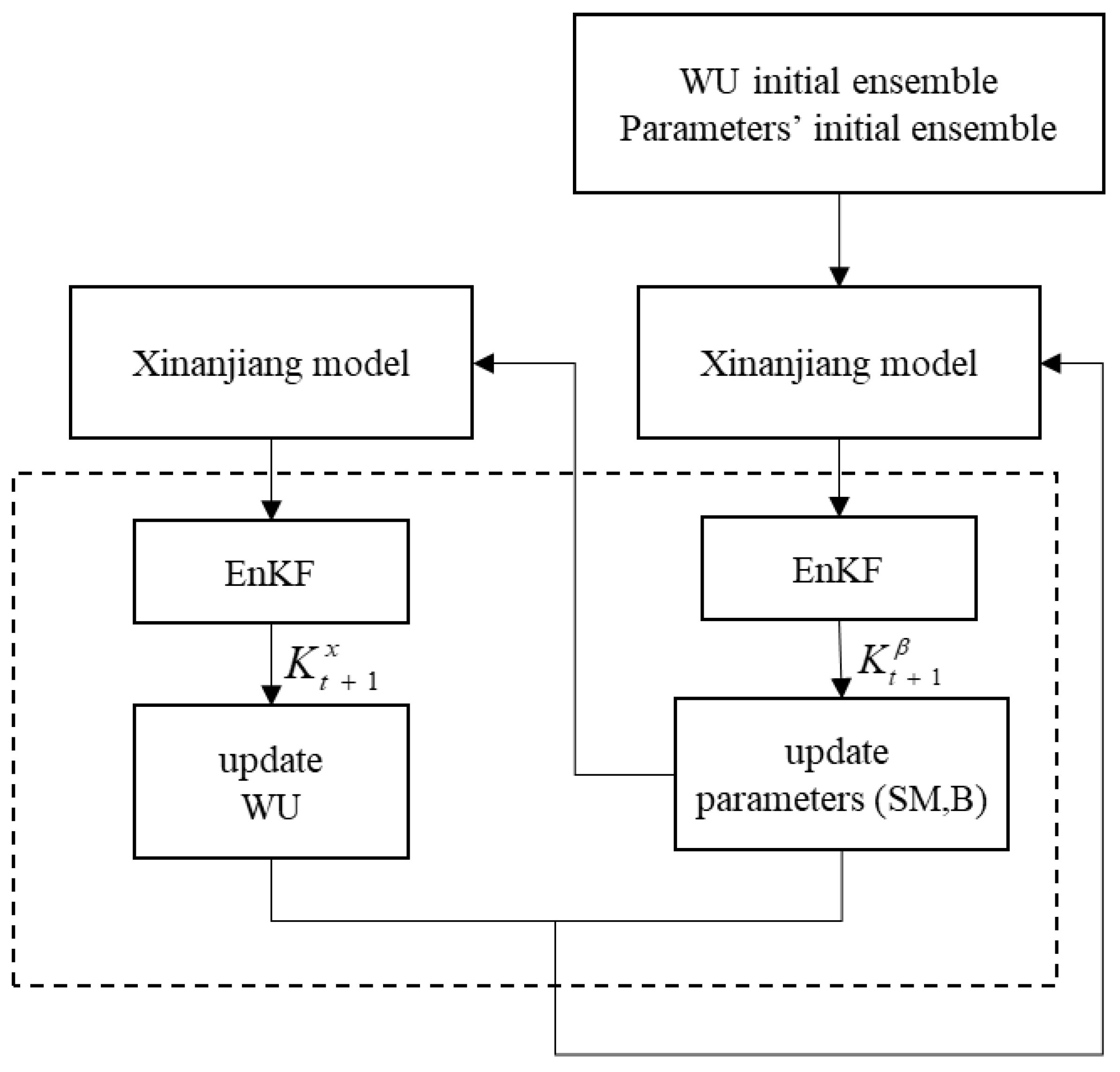
The dual ensemble Kalman filter (DEnKF) cycled through EnKF twice when estimating parameters and state variables at a certain time, and its algorithm diagram is shown in Figure 5. First, the parameter background was added to the model to predict the state variables. The filter gain of parameters $K_{t+1}^{\beta }$ was calculated when there were observations, and the parameter analysis ensemble $K_{t+1}^a$ was obtained. The parameter analysis ensemble was input to the model again at that moment to obtain the new prediction ensemble of state variables $X_{t+1}^a$. The DEnKF algorithm was divided into two filters to determine the optimal estimation of parameters and state variables. The optimal parameter obtained by the first filter was used to predict the state variables, and the optimal estimation of state variables was obtained by the second filter.

The two gains were calculated as follows:

$$K_{t+1}^{\beta }={{\displaystyle \sum }}_{t+1}^{\beta y}{[{{\displaystyle \sum }}_{t+1}^{yy}+{{\displaystyle \sum }}_{t+1}^y]}^{-1}$$

(13)

$$K_{t+1}^x={{\displaystyle \sum }}_{t+1}^{xy}{[{{\displaystyle \sum }}_{t+1}^{yy}+{{\displaystyle \sum }}_{t+1}^y]}^{-1}$$

(14)

where ${\sum }_{t+1}^{\beta y}$ is the covariance of the parameter with the state variable on the observed projection, ${\sum }_{t+1}^{xy}$ is the covariance of the state variable with the state variable on the observed projection, ${\sum }_{t+1}^{yy}$ is the variance of the state variable on the observed projection, and ${\sum }_{t+1}^y$ is the observation error.

It should be noted that the initial background was uniformly sampled in the parameter space. After parameters were updated each time, the parameter ensemble needed to be resampled using the kernel smoothing algorithm, as shown in Equation (15) [39]. This sampling method avoided the potential sample divergence and information loss, and ensured the stability of parameter assimilation. In addition, the parameter background error needed to be reflected by the function of the mean and variance of the parameter ensemble at the previous moment.

$${\beta }_{t+1}^i~N\left(\alpha {\beta }_t^i+\left(1-\alpha \right){\beta }_t,h^2{V}_t\right)$$

(15)

where $a=\frac{3\delta -1}{2\delta }$ and $\delta$ are in the range of 0 to 1, $h=\sqrt{1-a^2}$.

4. Results

4.1. Simulation of Xinanjiang Model

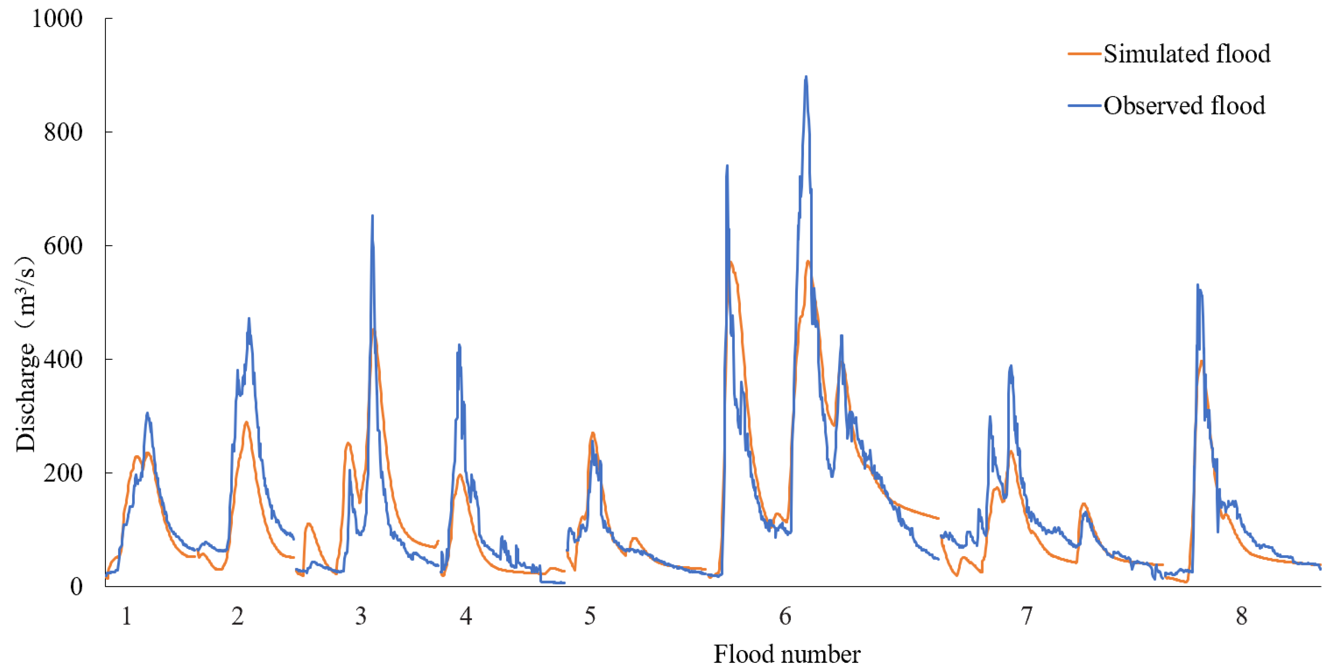
With NSE as the objective function, the model parameters were determined by the SCE-UA algorithm, in which the first 19 floods (1999–2013) were used for parameter calibration, and the last 8 floods (2017–2021) were applied for parameter verification. The flood peak relative error, peak time difference and NSE were used as indexes to evaluate the simulation results of the Xinanjiang model, as shown in

Table 5. Results of simulated floods in the Xinanjiang model (calibration period).

Flood Number	Flood Peak Relative Error	Peak Time Difference (h)	NSE
No. 19990705	0.31	0	0.860
No. 20000628	0.00	0	0.823
No. 20000713	0.36	1	0.815
No. 20000808	0.23	4	0.873
No. 20030716	0.17	0	0.898
No. 20030920	0.31	3	0.854
No. 20040930	0.16	3	0.882
No. 20050817	0.31	4	0.840
No. 20060927	0.01	4	0.943
No. 20070705	0.04	10	0.731
No. 20070720	0.14	0	0.835
No. 20090803	0.03	5	0.912
No. 20090819	0.14	1	0.703
No. 20090829	0.11	3	0.815
No. 20100608	0.01	7	0.872
No. 20109010	0.15	8	0.804
No. 20110622	0.28	4	0.851
No. 20110805	0.05	2	0.775
No. 20130719	0.08	5	0.853
Average	0.15	3.37	0.839

and

Table 6. Results of simulated floods in Xinanjiang model (validation period).

Flood Number	Flood Peak Relative Error	Peak Time Difference (h)	NSE
1 (No. 20170927)	0.23	0	0.846
2 (No. 20171004)	0.39	4	0.580
3 (No. 20180704)	0.31	2	0.622
4 (No. 20190628)	0.54	2	0.661
5 (No. 20190807)	0.06	0	0.805
6 (No. 20190915)	0.36	3	0.779
7 (No. 20200819)	0.39	1	0.604
8 (No. 20210424)	0.25	6	0.910
Average	0.32	2.25	0.725

, and Figure 6.

As can be seen from Table 6, the Xinanjiang model had applicability in the Xun River, and the floods simulated by this set of parameters fit well with actual floods. In the calibration period, the overall flood peak error and NSE of the simulated floods were 0.15 and 0.839, respectively, among which the flood peak error of 13 floods was within 0.2, and the peak time difference of more than half the floods was controlled within 3 h. The NSE of all floods was above 0.7, and the NSE of simulated floods closest to the measured flood was as high as 0.943.

It can be seen from Table 6 and Figure 6 that the Xinanjiang model had applicability in the runoff simulation of the Xun River. In the validation period, the overall flood peak error and NSE of the simulated floods were 0.32 and 0.725, and the peak time difference of most floods could be controlled within 3 h. The NSE of the simulated flood was as high as 0.910, which was closest to the measured value. However, generally speaking, the flood peak error was relatively large compared with the calibration period, and there were also unsatisfactory simulated floods with an NSE less than 0.7. Improving the prediction accuracy of such floods was the focus of subsequent data assimilation.

4.2. Assimilation Scheme of WU

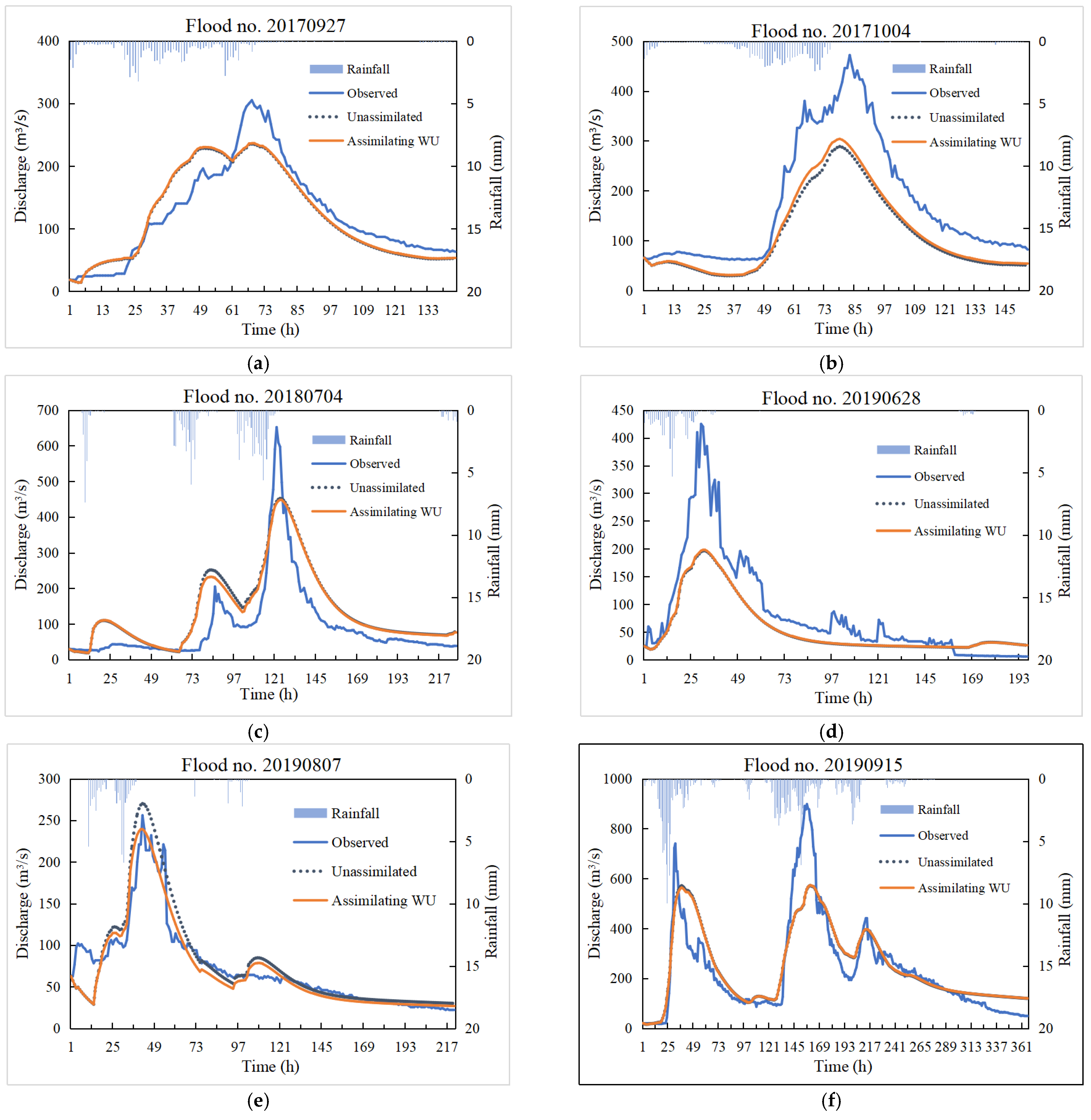
To explore the application effect of data assimlation in the flood prediction of the Xun River Basin above Chaiping, an assimilation scheme for soil moisture was proposed for eight floods during the validation period (2017–2021). The assimilation results were subsequently analyzed with the original simulations of the Xinanjiang model. The state variable in assimilating soil moisture was the WU of the Xinanjiang model, and the observation utilized SMAP remote sensing soil moisture data. The observation error variance was set as 1, and the initial error variance was set as 5. The mean value of the initial ensemble was taken as the soil moisture at the initial observation time to generate the initial background of WU, which was input to the Xinanjiang model to update WU through a continuous forward filter. The sample number N was set to 200. Based on the above settings, EnKF was used to assimilate the WU of the Xinanjiang model to explore its improvement effect on flood projection in the Xun River Basin above Chaiping, and the results are shown in

Table 7. Simulation results of assimilated WU.

Flood Number	Flood Peak Relative Error	Peak Time Difference (h)	NSE
1 (No. 20170927)	0.22	0	0.845
2 (No. 20171004)	0.36	3	0.655
3 (No. 20180704)	0.31	2	0.662
4 (No. 20190628)	0.53	2	0.668
5 (No. 20190807)	0.06	0	0.873
6 (No. 20190915)	0.36	3	0.781
7 (No. 20200819)	0.36	1	0.656
8 (No. 20210424)	0.22	5	0.924
Average	0.30	2	0.758

and Figure 7.

As can be seen from Table 7, assimilation after the addition of soil moisture data observed by remote sensing improved the prediction accuracy of the eight floods in the validation period to a certain extent. The overall flood peak relative error decreased from 0.32 to 0.3, NSE increased from 0.725 to 0.758, and the peak time difference also improved to a certain extent. The flood peak error of flood no. 20170927, flood no. 20171004, flood no. 20190628, flood no. 20200819 and flood no. 20210424 were all reduced, and the best decrease was by 3%. The peak time difference has been reduced by 1 h for flood no. 20171004 and flood no. 20210424. In terms of NSE, except for flood no. 20170927, which had a slight decrease (0.1%) after assimilation, the other floods all improved to a certain extent, increasing by 7.5%, at most.

On the whole, flood no. 20170927, flood no. 20190807 and flood no. 20210424 performed well in flood simulation, and the NSE reached above 0.8. As for the flood peak overestimation of flood no. 20190807, the possible reason was that the rainfall concentrated in the upper reaches of the basin after the area mean conversion did not take into account the flood attenuation. Although most flood peak errors are large, they basically reflect each flood peak. For multi-peak flooding, such as flood no. 20190915 and flood no. 20200819, although the largest flood peak for each was underestimated, there were smaller flood peaks whose simulations were very close to those observed. In general, the assimilation of WU was shown to improve the accuracy of flood prediction to a certain extent, but its ability was limited. In the future, SMAP remote sensing data could be combined with the soil moisture data measured at watershed stations or other remote sensing data to further explore the improvement of flood prediction by soil moisture assimilation.

4.3. Simultaneous Assimilation of Parameters and WU

The parameters applied in the previously established model were the optimal parameters obtained by SCE-UA using the historically measured floods. However, the parameters in the actual situation are often not definite values. They usually change with climate and underlying surface. It is not reliable to predict future floods with fixed parameters determined by historical hydrological data. In this paper, the scheme of assimilating WU was improved, i.e., the model parameters were assimilated and updated in the prediction process. Referring to the parameter sensitivity analysis of the Xinanjiang model performed by Lü, et al. [40], two sensitive parameters (i.e., soil storage capacity curve index (B) and basin average free water storage capacity (SM)) and WU were assimilated simultaneously in this paper.

WU was assimilated with the parameters B and SM simultaneously by augmented ensemble Kalman filter, and the corresponding AEnKF assimilation scheme has been proposed here. The obtained results are shown in

Table 8. Simulation results of AEnKF assimilation.

Flood Number	Flood Peak Relative Error	Peak Time Difference (h)	NSE
1 (No. 20170927)	0.21	0	0.825
2 (No. 20171004)	0.32	3	0.709
3 (No. 20180704)	0.39	3	0.763
4 (No. 20190628)	0.45	1	0.674
5 (No. 20190807)	0.07	1	0.872
6 (No. 20190915)	0.30	2	0.827
7 (No. 20200819)	0.29	1	0.655
8 (No. 20210424)	0.21	5	0.926
Average	0.28	2	0.781

.

As can be seen from Table 8, the ensemble Kalman filter assimilation considering the parameters and WU at the same time was shown to improve flood prediction accuracy. The overall NSE increased from 0.725 without assimilation, and 0.758 with assimilated WU, to 0.781, and the peak time difference also improved. After assimilation, the peak relative errors of the eight floods decreased to different degrees, except for flood no. 20180704 and flood no. 20190807. Compared with the unassimilated and assimilating WU schemes, the flood peak errors reduced by 9% and 8%, at most, respectively. The peak time difference between flood no. 20190628 and flood no. 20190915 decreased by 1 h compared with assimilating WU. The NSEs of all floods improved except for flood no. 20170927, which reduced by 2%. Compared with the unassimilated simulations by the Xinanjiang model, NSE increased by a maximum of 14.1%, and the number of floods with an NSE of 0.7 in the eight floods, increased from four to six. Compared with the simulations of WU assimilation, NSE increased by 10.1% at most, and the number of floods with NSE above 0.7 in the eight floods also increased by two.

On the whole, flood no. 20170927, flood no. 20190807, flood no. 20190915 and flood no. 20210424 performed well in flood simulation, and their NSEs reached above 0.8. The results showed that assimilating WU and model parameters SM and B by state variables expansion had a positive effect on the improvement of flood prediction accuracy.

The dual ensemble Kalman filter method was used to assimilate WU with parameters B and SM simultaneously, and the corresponding DEnKF assimilation scheme has also been proposed here. The obtained results are shown in

Table 9. Simulation results of DEnKF assimilation.

Flood Number	Flood Peak Relative Error	Peak Time Difference (h)	NSE
1 (No. 20170927)	0.21	0	0.822
2 (No. 20171004)	0.29	3	0.655
3 (No. 20180704)	0.42	3	0.772
4 (No. 20190628)	0.41	1	0.695
5 (No. 20190807)	0.09	1	0.874
6 (No. 20190915)	0.32	2	0.804
7 (No. 20200819)	0.31	1	0.692
8 (No. 20210424)	0.16	6	0.925
Average	0.27	2.125	0.779

.

It can be seen from Table 9 that the dual ensemble Kalman filter method better simulated the flood process by assimilating parameters and WU at the same time. The overall NSE increased from 0.725 for unassimilated, and 0.758 for assimilated WU, to 0.779, and the peak time difference also improved. Compared with the results of unassimilated and assimilating WU, the peak error with parameter updating reduced by 13% and 12%, at most, respectively. The peak time difference between the two floods was improved compared with assimilating WU. The NSEs of all floods improved except for flood no. 20170927, which reduced by about 2.3%. Compared with the results of unassimilated and WU assimilation, NSE improved by a maximum of 15% and 11%, respectively. The number of floods with NSE above 0.7 increased to five.

On the whole, flood no. 20170927, flood no. 20190807, flood no. 20190915 and flood no. 20210424 still performed well in flood simulation, and NSEs reached above 0.8. Combined with the results of the WU assimilation scheme, it was seen that the dual ensemble Kalman filter method effectively improved the accuracy of flood prediction by simultaneously assimilating parameters and WU.

4.4. Comparison of Results

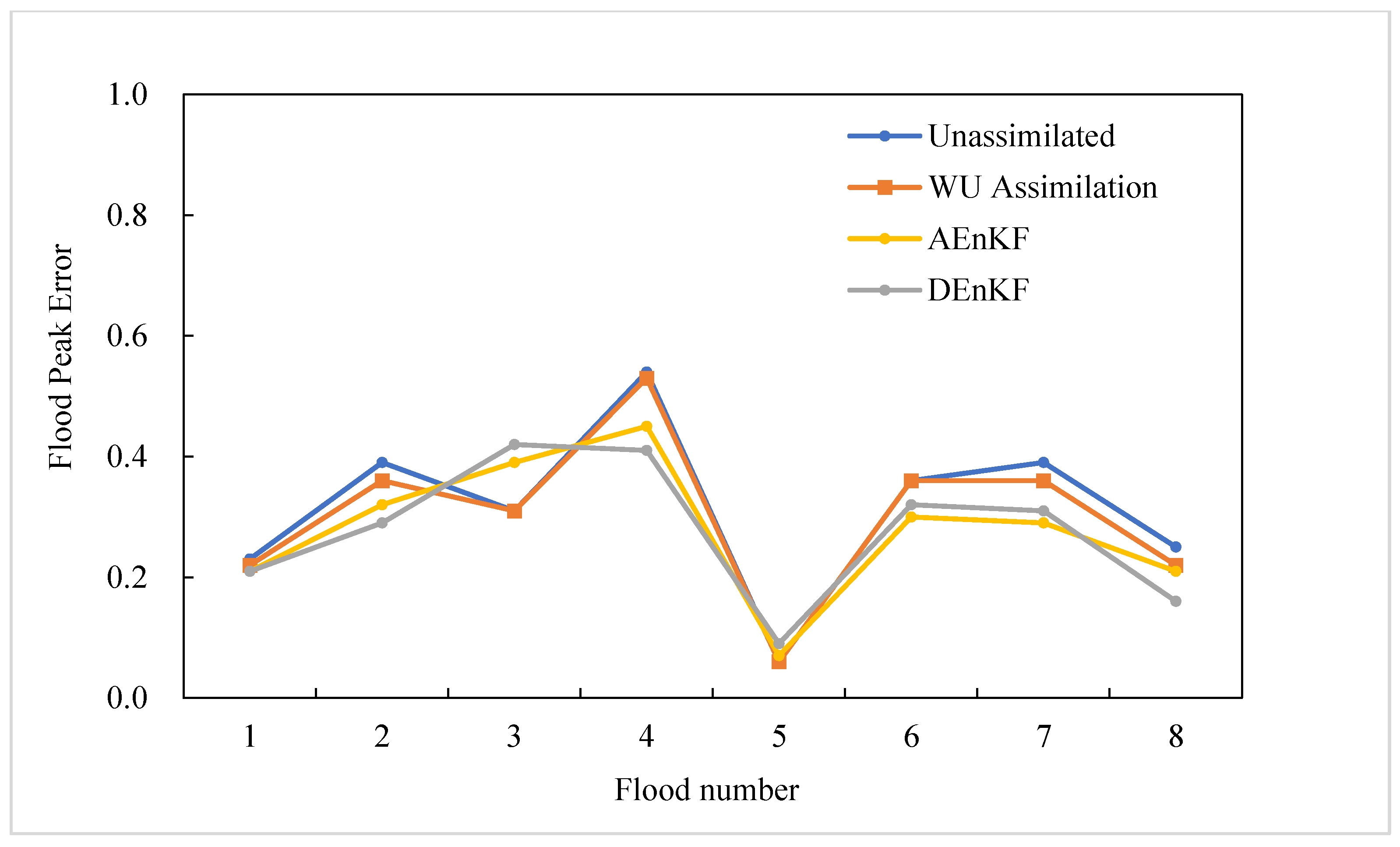
The two schemes (AEnKF scheme and DEnKF scheme) with simultaneous assimilation of parameters and state variables were compared with the simulations of the unassimilated scheme and WU assimilation scheme. The flood peak error of each scheme was calculated, as shown in

Table 10. Comparison of flood peak errors.

	Flood Peak Error	Unassimilated	WU Assimilation	AEnKF	DEnKF
Flood Number
1 (No. 20170927)		0.23	0.22	0.21	0.21
2 (No. 20171004)		0.39	0.36	0.32	0.29
3 (No. 20180704)		0.31	0.31	0.39	0.42
4 (No. 20190628)		0.54	0.53	0.45	0.41
5 (No. 20190807)		0.06	0.06	0.07	0.09
6 (No. 20190915)		0.36	0.36	0.30	0.32
7 (No. 20200819)		0.39	0.36	0.29	0.31
8 (No. 20210424)		0.25	0.22	0.21	0.16
Average		0.32	0.30	0.28	0.27

. The overall flood peak error of the four simulation schemes from large to small was: unassimilated, assimilated WU, AEnKF, and DEnKF, thus, proving that assimilating parameters and WU had a certain reduction effect on flood peak error. Compared with the unassimilated scheme, the overall flood peak error of assimilated WU was reduced by 2%, and the flood peak error of three floods was reduced by 3%. Compared with the results of WU assimilation, the flood peak errors of the two improved schemes decreased except for flood no. 20180704 and flood no. 20190807. In the AEnKF scheme and DEnKF scheme, the flood peak errors decreased by 8% and 12%, at most. Both of these considered parameter assimilation schemes reduced the flood peak error in more than half of floods by 4% or more.

Using the data in Table 10 to draw Figure 8, it can also be visually concluded that the flood peak errors, when assimilating parameters and WU simultaneously, were reduced to different degrees, compared with both unassimilated and WU assimilation. WU assimilation had little effect on flood peak error. The schemes with assimilating parameters reduced flood peak error and had a better assimilation effect. In general, the data assimilation method reduced the error of flood peak prediction, and the Xinanjiang model with simultaneous assimilation of parameters and state variables was better in flood peak prediction.

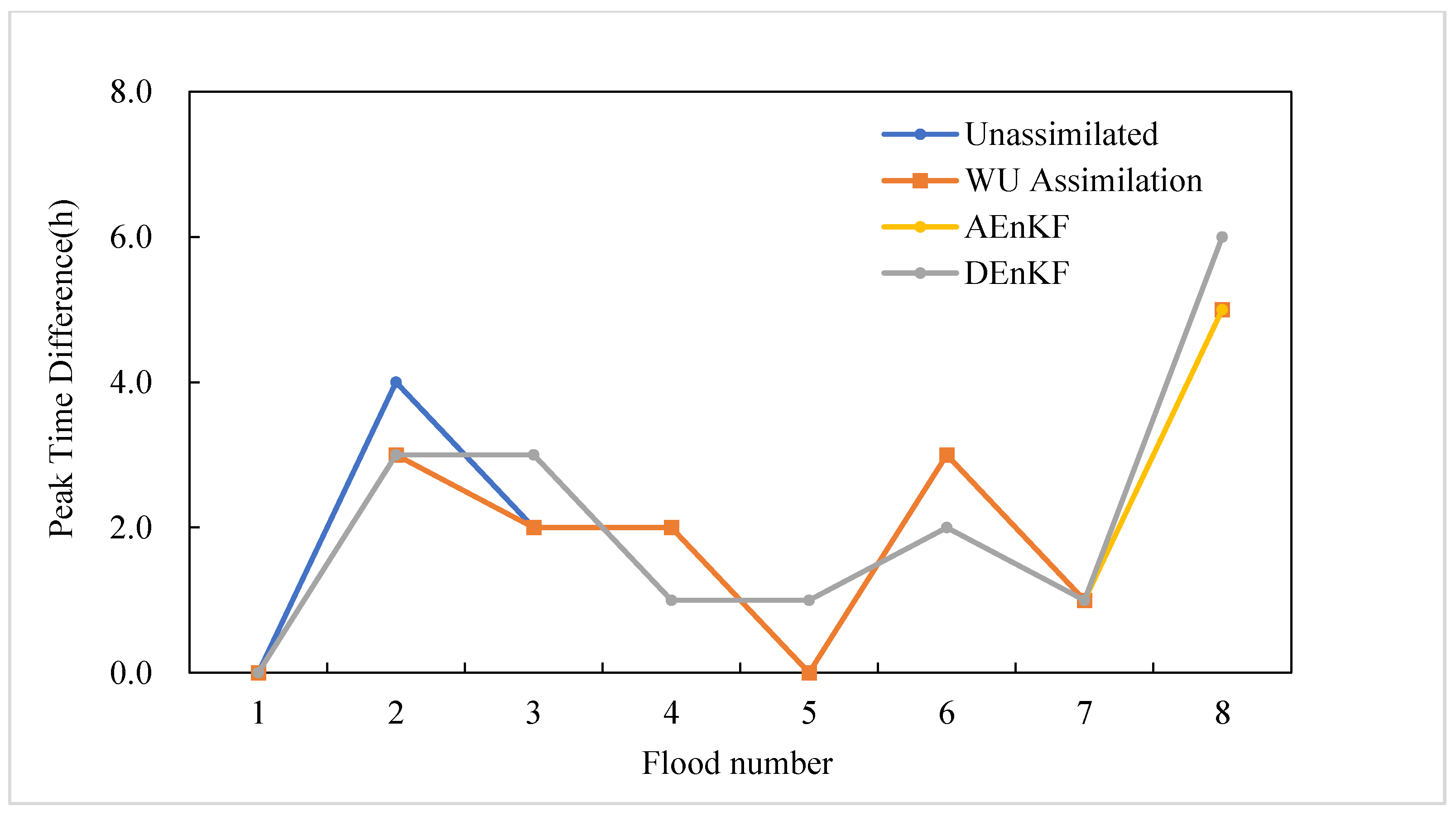
According to

Table 11. Comparison of peak time difference.

	Peak Time Difference (h)	Unassimilated	WU Assimilation	AEnKF	DEnKF
Flood Number
1 (No. 20170927)		0	0	0	0
2 (No. 20171004)		4	3	3	3
3 (No. 20180704)		2	2	3	3
4 (No. 20190628)		2	2	1	1
5 (No. 20190807)		0	0	1	1
6 (No. 20190915)		3	3	2	2
7 (No. 20200819)		1	1	1	1
8 (No. 20210424)		6	5	5	6

, the number of floods with a peak time difference exceeding 3 h was two in the unassimilated scheme, and one flood in the other three schemes, indicating that data assimilation played a role in reducing the flood peak time difference. The maximum peak time difference was 6 h in the unassimilated scheme. After assimilating WU, the peak time difference of flood no. 20171004 and flood no. 20210424 decreased by 1 h, respectively. After adding the parameter assimilation, the peak time differences of flood no. 20190628 and flood no. 20190915 were both reduced by 1 h.

Using the data in Table 11 to draw Figure 9, it can also be seen visually that with the addition of the parameter assimilation, the peak time difference of the AEnKF scheme was reduced in four and two floods, respectively, compared with those unassimilated and WU assimilation. The peak time difference of the DEnKF scheme compared with that of unassimilated and assimilating WU decreased in three and two floods, and both decreased by 1 h. In general, data assimilation predicted flood peak time closer to the actual situation.

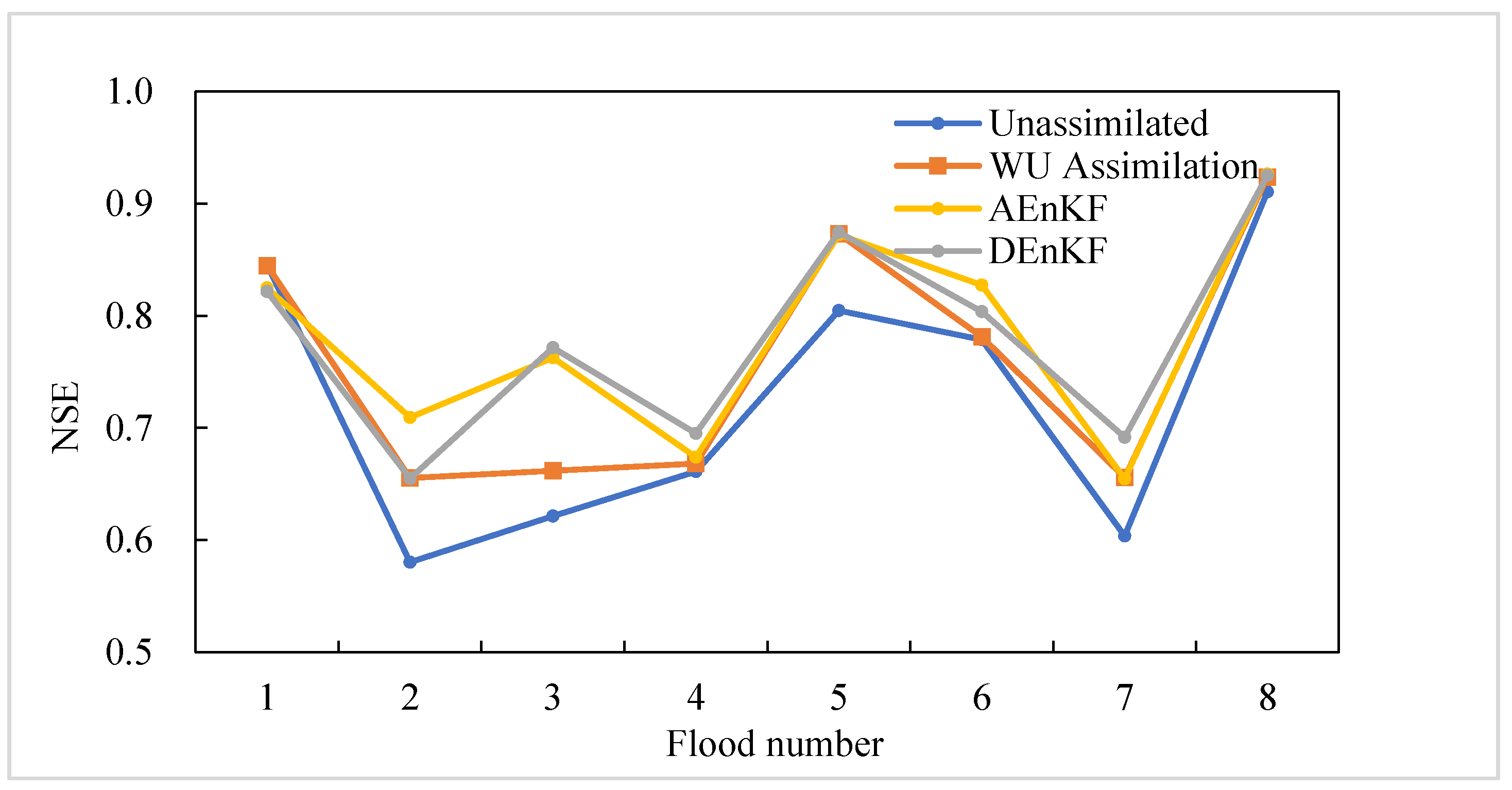
Through the NSE statistics of each scheme for each flood, it can be seen from

Table 12. Comparison of NSE.

	NSE	Unassimilated	WU Assimilation	AEnKF	DEnKF
Flood Number
1 (No. 20170927)		0.846	0.845	0.825	0.822
2 (No. 20171004)		0.580	0.655	0.709	0.655
3 (No. 20180704)		0.622	0.662	0.763	0.772
4 (No. 20190628)		0.661	0.668	0.674	0.695
5 (No. 20190807)		0.805	0.873	0.872	0.874
6 (No. 20190915)		0.779	0.781	0.827	0.804
7 (No. 20200819)		0.604	0.656	0.655	0.692
8 (No. 20210424)		0.910	0.924	0.926	0.925
Average		0.725	0.758	0.781	0.779

that the average NSE of the four simulation schemes, from large to small, were: AEnKF, DEnKF, WU assimilation and unassimilated. It proved that considering parameters and WU assimilation at the same time improved the accuracy of flood simulation. Compared with the unassimilated scheme, the overall NSE improved by 3.3% after assimilating WU. The NSE of flood no. 20171004 and flood no. 20190807 increased by 7.5% and 6.8%, respectively. Compared with the unassimilated and WU assimilation, the average NSE of eight floods in the AEnKF scheme increased by 5.6% and 2.3%, respectively, and those in DenKF increased by 5.4% and 2.1%, respectively. Compared with WU assimilation, the number of floods with NSE above 0.7 after adding parameters assimilation increased by two and one, respectively. For flood no. 20180704, NSE improved the most after considering parameters assimilation, with AEnKF increasing the NSE by 14.1% compared with unassimilated, by 10.1% compared with WU assimilation, and the DEnKF increasing NSE by 15% compared with unassimilated and by 11% compared with WU assimilation.

Using the data in Table 12 to draw Figure 10, it can also be visually concluded that, after assimilating WU with the observational data, the NSE of all floods except flood no. 20170927 improved, but some only had a small increase. Assimilation of model parameters and WU improved the NSE to a greater extent. Compared with assimilating WU, AEnKF had a better NSE improvement effect on flood no. 20171004 and flood no. 20180704, while DEnKF performed better on flood no. 20180704 and flood no. 20200819. On the whole, the improvement effect of AEnKF and DEnKF on NSE were similar, and NSE was improved to a certain extent compared with the unassimilated and WU assimilation schemes.

Root mean square error (RMSE) is another common indicator used to measure the deviation between model simulations and measured values when evaluating flood prediction. The RMSE can reflect the deviation between observation and prediction. The smaller it is, the closer the predicted value is to the measured value, and the better the prediction is, as shown in Equation (16):

$$\mathrm{RMSE}=\sqrt{\frac{{\sum }_{t=1}^T{\left(Q_o^t-Q_m^t\right)}^2}{T}}$$

(16)

where T is the total time duration (h) corresponding to each flood, $Q_o^t$ is the measured runoff at t, and $Q_m^t$ is the predicted runoff at t.

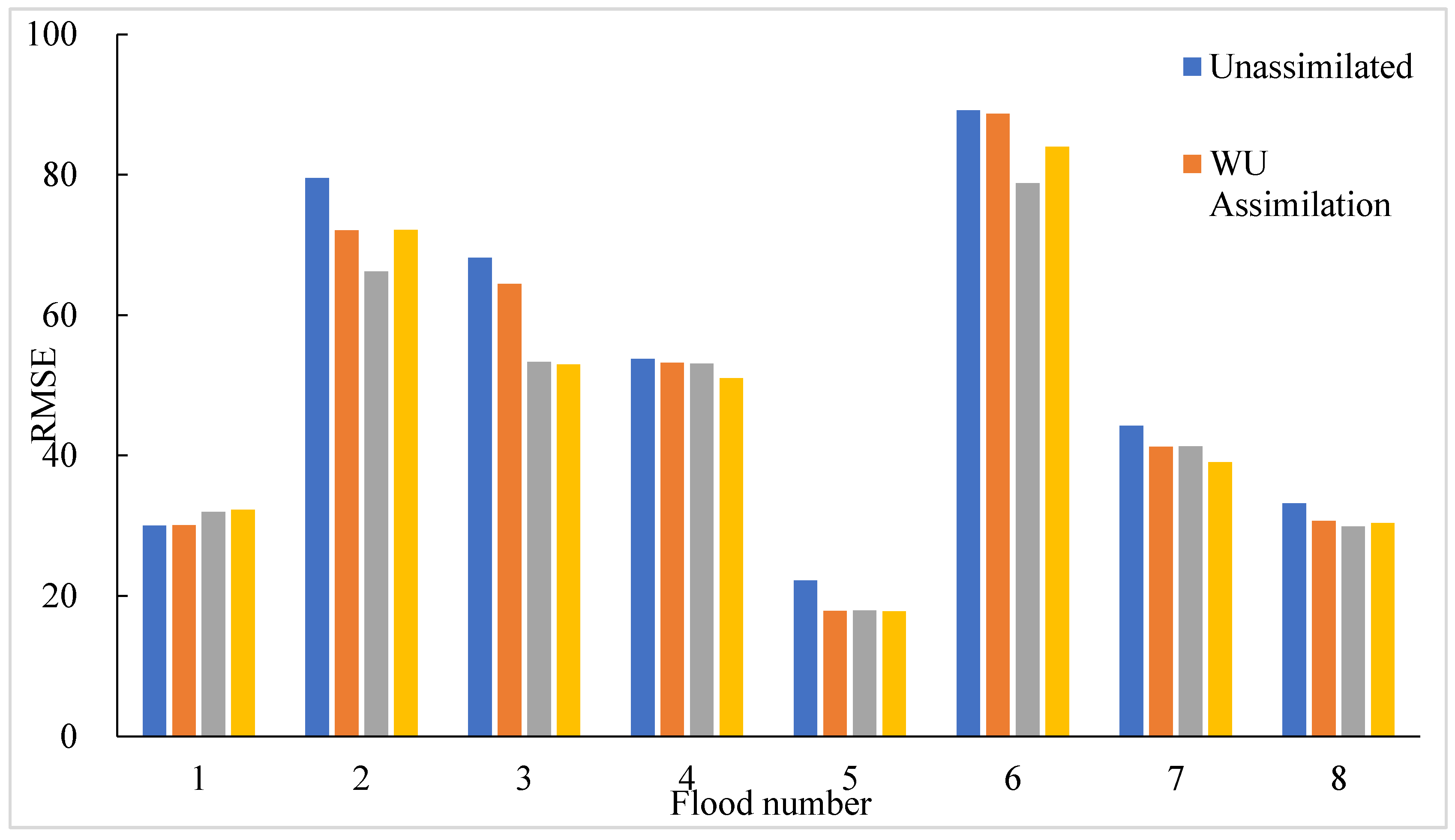
In this paper, the results of the above four simulation schemes were compared with the measured runoff data. The RMSE of runoff in each flood was counted, as shown in

Table 13. Root mean square error results of runoff (m³/s).

	RMSE	Unassimilated	WU Assimilation	AEnKF	DEnKF
Flood Number
1 (No. 20170927)		30.033	30.100	31.991	32.279
2 (No. 20171004)		79.529	72.073	66.196	72.111
3 (No. 20180704)		68.184	64.442	53.311	52.966
4 (No. 20190628)		53.793	53.216	53.069	51.032
5 (No. 20190807)		22.188	17.888	17.938	17.787
6 (No. 20190915)		89.175	88.673	78.769	83.995
7 (No. 20200819)		44.267	41.245	41.315	39.048
8 (No. 20210424)		33.213	30.685	29.884	30.376
Average		52.548	49.790	46.559	47.449

. Except that the RMSE of flood no. 20170927 increased slightly in the two schemes of assimilating parameters and WU, the RMSE of the other floods decreased to different degrees compared with WU assimilation. The overall RMSE from large to small was: unassimilated, assimilated WU, DEnKF and AEnKF scheme.

Figure 11 was drawn based on the RMSE of runoff for each flood in Table 10. It can also be seen visually that the simultaneous assimilation of model parameters and state variables effectively reduced model errors in flood prediction. Except for flood no. 20170927, the RMSE of the other floods all reached the maximum in the unassimilated scheme, which indicated that the prediction of the Xinanjiang model without assimilation was quite different from the measured data, and data assimilation was effective in improving the simulation accuracy. On the whole, the AEnKF scheme had a better flood prediction effect than DEnKF, and its average RMSE was smaller. By comparing the RMSEs of WU assimilation, DEnKF and AEnKF schemes, it could be seen that the schemes with dynamic parameter update performed better in reducing the runoff prediction errors.

5. Conclusions

The numerous uncertainties in flood projection models have limited the forecast accuracy, while data assimilation has been proved to improve the flood prediction accuracy by combining the prediction model with the actual observations. In addition, the development of remote sensing technology has broadened access to data, which provides more possibilities for the application of assimilation in flood projection. In this study, the Xun River of the Hanjiang River Basin was selected as the research object. The EnKF algorithm was applied to the Xinanjiang model, and a data assimilation scheme for the WU of the Xinanjiang model was proposed to explore the improvement effect of assimilation on the forecast accuracy. Thereafter, the WU assimilation scheme was further improved, and two novel assimilation schemes (AEnKF scheme and DEnKF scheme) were proposed to update the model-sensitive parameters and WU simultaneously. The main conclusions are as follows.

(1) Using SMAP remote-sensing soil moisture data, WU assimilation improved the flood forecast accuracy to some extent. The overall flood peak error of the eight floods in the validation period decreased from 0.32 to 0.3, the NSE improved from 0.725 to 0.758, and the peak time difference also improved to a certain extent. The flood peak error of flood no. 20170927, flood no. 20171004, flood no. 20190628, flood no. 20200819 and flood no. 20210424 improved, and the flood peak error decreased by 3% at most. The peak time difference of flood no. 20171004 and flood no. 20210424 were each reduced by 1 hour. In terms of the NSE, except for flood no. 20170927, whose NSE had a slight decrease (0.1%), all the other floods improved to some extent, and NSE was increased by 7.5%, at most;

(2) The dynamic update of model parameters during the projection process was more realistic than taking fixed values. Compared with the WU assimilation scheme, the simultaneous assimilation of parameters and WU effectively improved the prediction ability of the Xinanjiang model. The AEnKF scheme improved the overall NSE of flood from 0.725 for unassimilated, and 0.758 for assimilated WU, to 0.781. Compared with the unassimilated simulation results, NSE increased by 14.1%, at most. In comparison with the results of assimilating WU, NSE improved by 10.1% at most, and the number of floods with NSE above 0.7 increased by two. The overall NSE of flood in the DEnKF scheme was improved to 0.779, and it was close to that of the AEnKF scheme. Compared with the results of unassimilated and WU assimilation, the flood peak errors after considering the parameter update reduced by 13% and 12% at most, respectively, and the NSE improved by a maximum of 15% and 11%, respectively. The above results indicated that the two improved schemes with simultaneous assimilation of model parameters and WU performed better in terms of improvement of forecast accuracy compared with the assimilating WU scheme.

References

- Chou, J.M.; Xian, T.; Dong, W.J.; Xu, Y. Regional Temporal and Spatial Trends in Drought and Flood Disasters in China and Assessment of Economic Losses in Recent Years. Sustainability 2019, 11, 55. [Google Scholar] [CrossRef] [Green Version]
- Huang, C.C.; Pang, J.L.; Zha, X.C.; Su, H.X.; Jia, Y.F.; Zhu, Y.Z. Impact of monsoonal climatic change on Holocene overbank flooding along Sushui River, middle reach of the Yellow River, China. Quat. Sci. Rev. 2007, 26, 2247–2264. [Google Scholar] [CrossRef]
- Yin, J.F.; Gu, H.D.; Liang, X.D.; Yu, M.; Sun, J.S.; Xie, Y.X.; Li, F.; Wu, C. A Possible Dynamic Mechanism for Rapid Production of the Extreme Hourly Rainfall in Zhengzhou City on 20 July 2021. J. Meteorol. Res. 2022, 36, 6–25. [Google Scholar] [CrossRef]
- Han, S.S.; Coulibaly, P. Bayesian flood forecasting methods: A review. J. Hydrol. 2017, 551, 340–351. [Google Scholar] [CrossRef]
- Devi, G.K.; Ganasri, B.P.; Dwarakish, G.S. A Review on Hydrological Models. In Proceedings of the International Conference on Water Resources, Coastal and Ocean Engineering (ICWRCOE), Mangalore, India, 11–14 March 2015; pp. 1001–1007. [Google Scholar]
- Crawford, N.H.; Burges, S.J. History of the Stanford watershed model. Water Resour. Impact 2004, 6, 3–6. [Google Scholar]
- Fedora, M.A.; Beschta, R.L. Storm runoff simulation using an antecedent precipitation index (API) model. J. Hydrol. 1989, 112, 121–133. [Google Scholar] [CrossRef]
- Ren-Jun, Z. The Xinanjiang model applied in China. J. Hydrol. 1992, 135, 371–381. [Google Scholar] [CrossRef]
- Vrugt, J.A.; Diks, C.G.; Gupta, H.V.; Bouten, W.; Verstraten, J.M. Improved treatment of uncertainty in hydrologic modeling: Combining the strengths of global optimization and data assimilation. Water Resour. Res. 2005, 41. [Google Scholar] [CrossRef]
- Gupta, H.V.; Sorooshian, S.; Yapo, P.O. Status of automatic calibration for hydrologic models: Comparison with multilevel expert calibration. J. Hydrol. Eng. 1999, 4, 135–143. [Google Scholar] [CrossRef]
- Yi, S.L.; Zorzi, M. Robust Kalman Filtering Under Model Uncertainty: The Case of Degenerate Densities. IEEE Trans. Autom. Control. 2022, 67, 3458–3471. [Google Scholar] [CrossRef]
- Chao, Z.; Hua-sheng, H.; Wei-min, B.; Luo-ping, Z. Robust recursive estimation of auto-regressive updating model parameters for real-time flood forecasting. J. Hydrol. 2008, 349, 376–382. [Google Scholar] [CrossRef]
- Guo, S.; Xu, G.; Zhang, H.; Li, C. A Real-Time Flood Updating Model Based on the Bayesian Method; IAHS Press: Wallingford, UK, 2007; pp. 210–215. [Google Scholar]
- Liu, Z.; Guo, S.; Zhang, H.; Liu, D.; Yang, G. Comparative study of three updating procedures for real-time flood forecasting. Water Resour. Manag. 2016, 30, 2111–2126. [Google Scholar] [CrossRef]
- Ricci, S.; Piacentini, A.; Thual, O.; Le Pape, E.; Jonville, G. Correction of upstream flow and hydraulic state with data assimilation in the context of flood forecasting. Hydrol. Earth Syst. Sci. 2011, 15, 3555–3575. [Google Scholar] [CrossRef] [Green Version]
- Wu, X.-L.; Xiang, X.-H.; Wang, C.-H.; Chen, X.; Xu, C.-Y.; Yu, Z. Coupled hydraulic and Kalman filter model for real-time correction of flood forecast in the three gorges interzone of Yangtze river, China. J. Hydrol. Eng. 2013, 18, 1416–1425. [Google Scholar] [CrossRef]
- Si, W.; Bao, W.; Gupta, H.V. Updating real-time flood forecasts via the dynamic system response curve method. Water Resour. Res. 2015, 51, 5128–5144. [Google Scholar] [CrossRef]
- Muñoz, D.F.; Abbaszadeh, P.; Moftakhari, H.; Moradkhani, H. Accounting for uncertainties in compound flood hazard assessment: The value of data assimilation. Coast. Eng. 2022, 171, 104057. [Google Scholar] [CrossRef]
- Walker, J.P.; Houser, P.R. Hydrologic data assimilation. In Advances in Water Science Methodologies; CRC Press: Boca Raton, FL, USA, 2005; pp. 25–48. [Google Scholar]
- Welch, G.; Bishop, G. An Introduction to the Kalman Filter; University of North Carolina at Chapel Hill: Chapel Hill, NC, USA, 1995. [Google Scholar]
- Li, Q.; Li, R.; Ji, K.; Dai, W. Kalman filter and its application. In Proceedings of the 2015 8th International Conference on Intelligent Networks and Intelligent Systems (ICINIS), Tianjin, China, 1–3 November 2015; pp. 74–77. [Google Scholar]
- Evensen, G. Sequential data assimilation with a nonlinear quasi-geostrophic model using Monte Carlo methods to forecast error statistics. J. Geophys. Res. Ocean. 1994, 99, 10143–10162. [Google Scholar] [CrossRef]
- Reichle, R.H.; McLaughlin, D.B.; Entekhabi, D. Hydrologic data assimilation with the ensemble Kalman filter. Mon. Weather. Rev. 2002, 130, 103–114. [Google Scholar] [CrossRef]
- Reichle, R.H.; Walker, J.P.; Koster, R.D.; Houser, P.R. Extended versus ensemble Kalman filtering for land data assimilation. J. Hydrometeorol. 2002, 3, 728–740. [Google Scholar] [CrossRef]
- Zhang, S.; Li, H.; Zhang, W.; Qiu, C.; LI, X. Estimating the soil moisture profile by assimilating near-surface observations with the ensemble Kaiman filter (EnKF). Adv. Atmos. Sci. 2005, 22, 936–945. [Google Scholar]
- Shen, Y.; Li, H.; Li, T.; Li, W. Groundwater level forecast: Overview of application of the Ensemble Kalman filter(EnKF). Hydrogeol. Eng. Geol. 2014, 41, 21–24. [Google Scholar]
- Li, X.-L.; Lü, H.; Horton, R.; An, T.; Yu, Z. Real-time flood forecast using the coupling support vector machine and data assimilation method. J. Hydroinform. 2014, 16, 973–988. [Google Scholar] [CrossRef] [Green Version]
- Wang, Z.; Lu, W.; Chang, Z.; Wang, H. Simultaneous identification of groundwater contaminant source and simulation model parameters based on an ensemble Kalman filter—Adaptive step length ant colony optimization algorithm. J. Hydrol. 2022, 605, 127352. [Google Scholar] [CrossRef]
- Tavakol, A.; McDonough, K.R.; Rahmani, V.; Hutchinson, S.L.; Hutchinson, J.S. The soil moisture data bank: The ground-based, model-based, and satellite-based soil moisture data. Remote Sens. Appl. Soc. Environ. 2021, 24, 100649. [Google Scholar] [CrossRef]
- Chan, S.K.; Bindlish, R.; Neill, P.E.O.; Njoku, E.; Jackson, T.; Colliander, A.; Chen, F.; Burgin, M.; Dunbar, S.; Piepmeier, J.; et al. Assessment of the SMAP Passive Soil Moisture Product. IEEE Trans. Geosci. Remote Sens. 2016, 54, 4994–5007. [Google Scholar] [CrossRef]
- Kerr, Y.H.; Waldteufel, P.; Richaume, P.; Wigneron, J.P.; Ferrazzoli, P.; Mahmoodi, A.; Al Bitar, A.; Cabot, F.; Gruhier, C.; Juglea, S.E. The SMOS soil moisture retrieval algorithm. IEEE Trans. Geosci. Remote Sens. 2012, 50, 1384–1403. [Google Scholar] [CrossRef]
- Zhao, R.; Liu, X. Computer models of watershed hydrology. In The Xinanjiang Model; Water Resources Publications: Littleton, CO, USA, 1995; pp. 215–232. [Google Scholar]
- Jayawardena, A.; Zhou, M. A modified spatial soil moisture storage capacity distribution curve for the Xinanjiang model. J. Hydrol. 2000, 227, 93–113. [Google Scholar] [CrossRef]
- Duan, Q.; Sorooshian, S.; Gupta, V. Effective and efficient global optimization for conceptual rainfall-runoff models. Water Resour. Res. 1992, 28, 1015–1031. [Google Scholar] [CrossRef]
- Zhang, C.; Jiang, J. Research on the application of SCE-UA algorithm for automatic parameters optimization of Xin’anjiang model. J. China Three Gorges Univ. 2020, 42, 18–23. [Google Scholar]
- Evensen, G. Data Assimilation: The Ensemble Kalman Filter; Springer: New York, NY, USA, 2009; Volume 2. [Google Scholar]
- Monsivais-Huertero, A.; Graham, W.D.; Judge, J.; Agrawal, D. Effect of simultaneous state–parameter estimation and forcing uncertainties on root-zone soil moisture for dynamic vegetation using EnKF. Adv. Water Resour. 2010, 33, 468–484. [Google Scholar] [CrossRef]
- Xie, X.; Zhang, D. Data assimilation for distributed hydrological catchment modeling via ensemble Kalman filter. Adv. Water Resour. 2010, 33, 678–690. [Google Scholar] [CrossRef]
- Moradkhani, H.; Sorooshian, S.; Gupta, H.V.; Houser, P.R. Dual state–parameter estimation of hydrological models using ensemble Kalman filter. Adv. Water Resour. 2005, 28, 135–147. [Google Scholar] [CrossRef] [Green Version]
- Lü, H.; Hou, T.; Horton, R.; Zhu, Y.; Chen, X.; Jia, Y.; Wang, W.; Fu, X. The streamflow estimation using the Xinanjiang rainfall runoff model and dual state-parameter estimation method. J. Hydrol. 2013, 480, 102–114. [Google Scholar] [CrossRef]
Figure 1.
The watershed above Chaiping Station in Xun River.
Figure 2.
Raw raster map of SMAP soil moisture data (red area is the study area).
Figure 3.
Raster map of the watershed above Chaiping after cropping.
Figure 4.
Flow diagram of AEnKF.
Figure 5.
Flow diagram of DEnKF.
Figure 6.
The chart of a simulated flood in the Xinanjiang model (validation period).
Figure 7.
Assimilation of WU.
Figure 8.
Comparison of flood peak errors for each flood of each scheme.
Figure 9.
Comparison of peak time difference for each flood of each scheme.
Figure 10.
Comparison of NSE for each flood of each scheme.
Figure 11.
Comparison of RMSE of runoff for each flood of each scheme.