


Numerical Modelling of an Innovative Conical Pile Head Breakwater
by
 , , , and
Arunakumar Hunasanahally Sathyanarayana
1 ,
,
Praveen S. Suvarna
2,
Pruthviraj Umesh
1,
Kiran G. Shirlal
1,
Hans Bihs
3 and
Arun Kamath
3,* 1
Department of Water Resources and Ocean Engineering, NITK Surathkal, Mangaluru 575025, Karnataka, India
2
Department of Civil Engineering, PACE, Mangaluru 575018, Karnataka, India
3
Department of Civil and Environmental Engineering, Norwegian University of Science and Technology, 7491 Trondheim, Norway
*
Author to whom correspondence should be addressed.
Water 2022, 14(24), 4087; https://doi.org/10.3390/w14244087
Submission received: 15 November 2022
/
Revised: 5 December 2022
/
Accepted: 9 December 2022
/
Published: 14 December 2022
(This article belongs to the Special Issue Computational Methods for Ocean Wave Interaction with Marine Structures)
Abstract
:When moderate wave activity at the shoreline is acceptable, pile breakwaters can serve as an alternative to conventional breakwaters. Increasing the size of the pile breakwater in the vicinity of the free surface increases the hydraulic efficiency, as most of the wave energy is concentrated around the free surface. Therefore, a conical pile head breakwater (CPHB) is proposed in the present study by gradually widening the diameter of the piles towards the free surface. Using the open-source computational fluid dynamics (CFD) model REEF3D, the transmission, reflection, and dissipation characteristics of the CPHB with monochromatic and irregular waves are examined. The investigation is carried out for both perforated and non-perforated CPHBs using monochromatic waves, and the numerical results are validated using experimental data. Further, optimally configured non-perforated and perforated CPHBs are investigated numerically by subjecting them to irregular waves using the Scott–Wiegel spectrum. The wave attenuation characteristics of the CPHBs are found to be better with irregular waves compared to monochromatic waves. With irregular waves, the minimum transmission coefficients for non-perforated and perforated CPHBs are 0.36 and 0.34, respectively. Overall, the CPHB appears to be a potential solution for coastal protection.
1. Introduction
Constructing breakwaters to provide partial or complete protection from waves is the key concept in coastal engineering for a variety of purposes, including coastal infrastructure protection, erosion management, and beach realignment. For some coastal facilities, such as fishing harbours, recreational harbours, oil jetties, and marinas, partial wave attenuation is sufficient. A certain extent of wave activity is desirable in coastal protection work to facilitate some sediment motion to maintain the dynamic equilibrium of beaches. Traditional breakwaters such as rubble mound and caisson breakwaters may not be an economical solution in these cases due to the massiveness of the structure. In such cases, the pile breakwater is an alternative that is capable of sheltering the coastal area to a reasonable extent.
Pile breakwaters are non-gravity structures composed of single or several rows of prismatic circular piles that are equally spaced. Pile breakwaters maintain the water quality of the sheltered area with minimal interference to sediment movement and do not hamper the aesthetics of the beach [1]. The attenuation of wave energy is mainly due to the obstruction, turbulence, vortex shedding and reflection around the structure during the wave–structure interaction. The wave–structure interaction occurs while the projected area of piles obstructs a major portion of the wave propagation. The small gap between the piles offers a narrow passage for the remaining portion of the wave to propagate, where the waves have to squeeze themselves. This concept has been innovatively used to discover new types of breakwaters, such as floating box structures [2]. The pile breakwater partially dissipates and partially transmits the incident wave energy with minimal reflection. Reflection from coastal structures may sometimes be important depending upon the site conditions that need to be curbed. This goal can be achieved by an innovative Bragg breakwater [3].
Pile breakwater structures have been constructed around the globe and are seen to be working effectively. Some of examples of existing pile breakwater structures are a reinforced concrete pile breakwater at Hanstholm, Denmark; closely spaced cylinder shells at Marsa el Brega, Libya; a steel pipe breakwater at the Port of Osaka, Japan; a concrete pipe breakwater at Pass Christian, Mississippi [4]; closely spaced piles at Half Moon Bay Marina, New Zealand [5]; a steel pipe breakwater at Pelangi Beach Resort, Malaysia [6]; sheet pile breakwaters at Bay St. Louis, USA; an interlocking type pipe breakwater at the Port of Ust-Luga, Russia; a steel pipe breakwater at Tanah Merah, Singapore [7]; and Zhoushan Islands, east China [8].
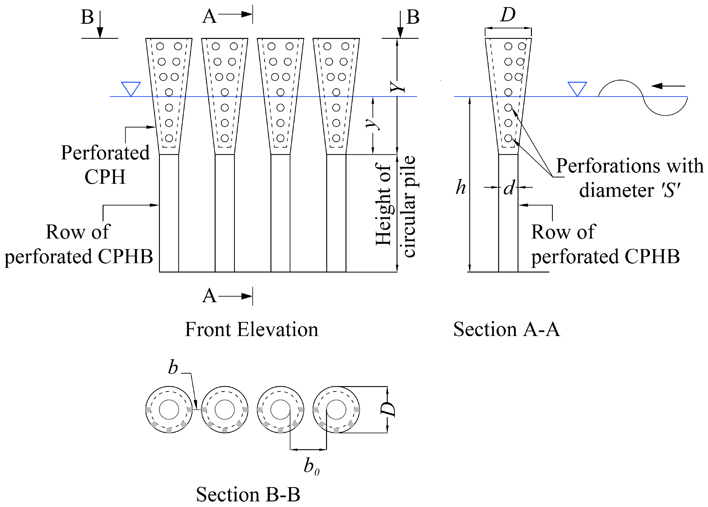
Many studies [1,9,10,11,12,13,14] have been conducted to assess the effectiveness of pile breakwaters. The results reveal that the wave transmission characteristics are directly proportional to the distance between the piles. Additionally, the transmission characteristics are inversely proportional to the incident wave steepness, the number of rows and the pile diameter. Van Weele et al. [15] demonstrated that a staggered pile arrangement resulted in higher wave attenuation and lower reflection. Several researchers [16,17,18,19,20] have identified that the efficiency of the pile breakwater can be increased by increasing the cross-sectional area of the structure near the free surface where most of the wave energy is concentrated. However, studies carried out to evaluate the hydraulic performance of pile breakwaters with an increased area at the top of the pile are scanty. In this context, the present study aims to bridge the existing knowledge gap by proposing innovative pile breakwaters. The cross-section of the pile breakwater is increased gradually near the free surface, as illustrated in Figure 1. This structure is designated as a conical pile head breakwater (CPHB). The enlarged area at the top is known as the conical pile head (CPH). Due to the increased area of the obstruction compared to a conventional pile breakwater, additional energy losses are expected to occur along with reduced wave transmission. The additional energy losses may occur due to the intense flow between the CPH, vortex formation, turbulence and reflection. The CPH is made hollow so that water can enter the conical structure, interact, and flush out after energy damping, resulting in further energy loss and reduced transmission. Basic modification of piles by itself without any additional components to dissipate wave energy is the novel concept of this study.
Perforated pile structures are found to be superior in wave attenuation compared to non-perforated structures by about 12 to 15% due to enhanced wave energy losses [21,22,23,24,25,26]. Therefore, this study also examines the influence of seaside perforations on the CPH (refer to Figure 1). In this study, the wave transmission coefficient (Kt), reflection coefficient (Kr) and dissipation coefficient (Kd) of non-perforated and perforated CPHBs are examined using the computational fluid dynamics (CFD) model REEF3D with both monochromatic and irregular waves. Before carrying out the numerical modelling of the CPHB, a sensitivity analysis is carried out to determine the optimal grid size and CFL number for accurate representation of waves. First, simulations on non-perforated and perforated CPHBs are performed using monochromatic waves. The numerical results are validated with experimental data [27,28], and the most efficient structural CPHB configurations are chosen. Further, the performance of the efficient CPHB models is examined with irregular waves. Finally, the performance characteristics with both types of waves are compared.
2. Modelling of CPHB Structure
2.1. Details of Physical Modelling
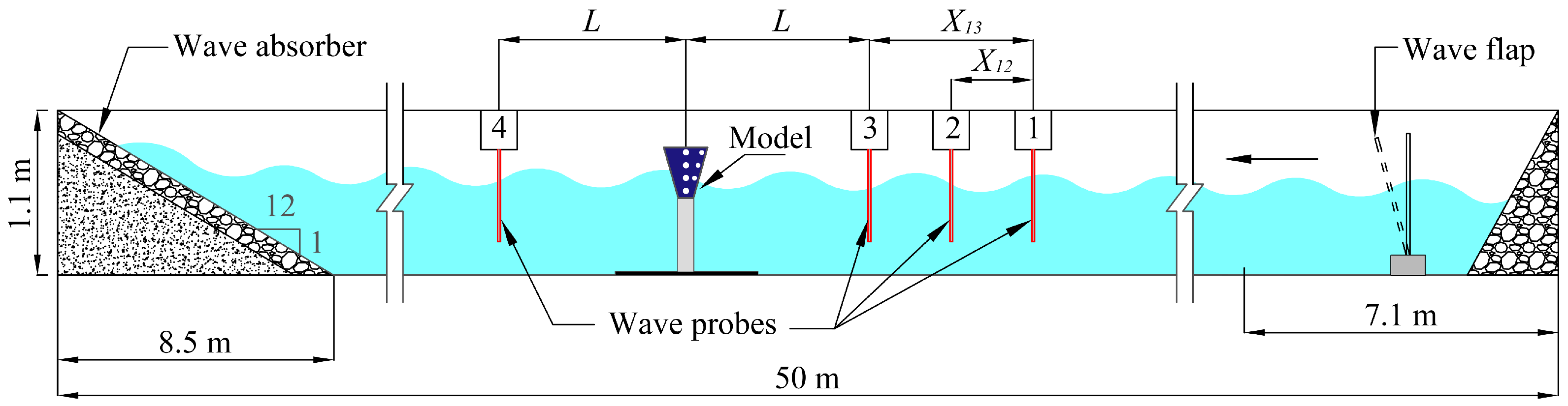
In order to validate the numerical results in the present work, the results are compared to the observations from physical model studies on non-perforated CPHBs [27] and perforated CPHBs [28]. The physical modelling studies were carried out in a wave flume (50 m × 0.71 m × 1.1 m) at the NITK Surathkal experimental facility in India. As the CPHB structure deals with surface waves, the modelling was carried out on a 1:30 scale employing Froude’s law. According to Froude’s law, gravity serves as the primary physical force counteracting the inertial force, and the influence of other physical forces is minimal. This may lead to scale effects when other forces, such as viscous forces, are dominant in the problem. However, viscous scale effects are expected to be minimal in this study, as the CPHB was tested under non-breaking wave conditions and the Reynolds numbers were always in the totally turbulent flow range [29]. The viscosity scale effects of the CPHB structure were evaluated by calculating the Reynolds number as described by Sarpkaya [30]. Additionally, the CPHB structure allows a considerable portion of the waves to enter the hollow region of the pile head. Hence, the potential viscous scale effect may be very minimal and can be neglected [31].
Monochromatic waves were generated using a bottom-hinged flap-type wave-maker, and the transmitted wave energy was absorbed by the wave absorber. An illustration of the physical wave tank along with the details of wave gauge placement are presented in Figure 2. A total of four wave gauges (WG) were used for logging the wave data. Three gauges were placed on the seaward side of the structure as per the three-probe methodology proposed by Isaacson [32] to calculate wave reflection. WG2 and WG3 were placed at a distance of L/3 and 2L/3, respectively, with reference to WG1, i.e., X12 = L/3 and X13 = 2L/3. The position of the gauges was adjusted in relation to the wavelength (L) of each generated wave. Using the three-probe approach [32], the composite wave data recorded in three gauges were separated into incident and reflected wave components (Hi and Hr, respectively). The transmitted wave height (Ht) was measured using WG4, which was located at a distance of ‘L’ from the structure. Further, an additional wave gauge (WG5) was employed to collect the wave data before placing the structure. These data were used for wave reconstruction in the numerical wave tank.
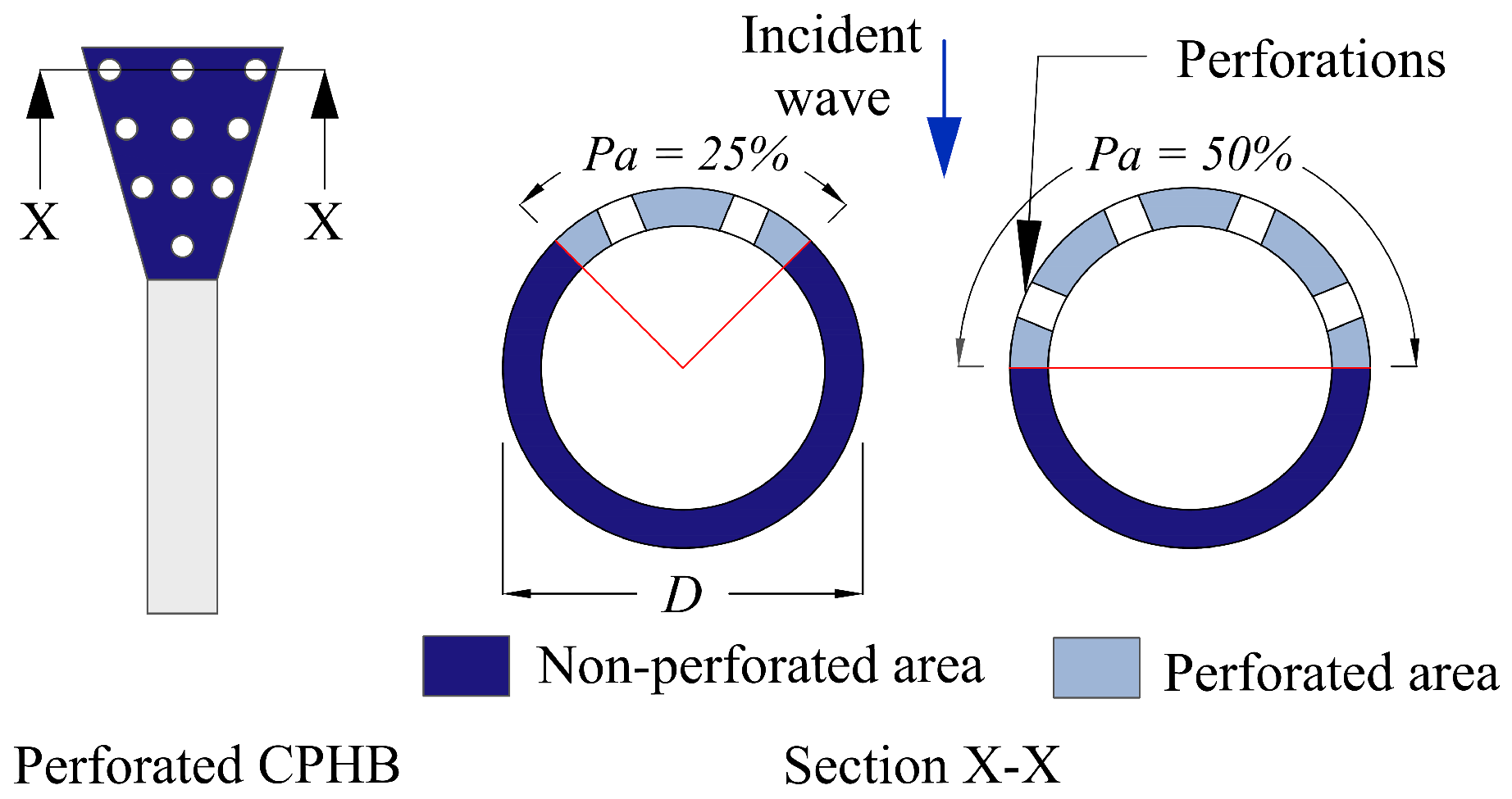
The CPHB structure was modelled by placing the hollow CPH on the supporting circular pile by means of a bolted connection, as presented in Figure 1. The supporting piles were fabricated with hollow galvanised iron pipes of 0.002 m thickness, and CPHs were 3D-printed using polylactic acid (PLA) material. The bottom of the supporting piles was firmly connected to a 0.01 m thick metal plate placed at the bottom of the flume, which replicates firm support at the seabed. Sathyanarayana et al. [27] carried out experiments on non-perforated CPHB by varying relative spacing between the pile heads (b/D) and relative diameter (D/Hmax) and height of the pile heads (Y/Hmax) with different wave climates. The study found that b/D = 0.1, D/Hmax = 0.4 and Y/Hmax = 1.5 is the optimum configuration in terms of wave attenuation. Further, Sathyanarayana et al. [28] introduced perforations on the optimum CPHB and investigated the influence of perforation distribution (Pa), percentage of perforations (P) and relative size of perforations (S/D). The typical tabulation of Pa is illustrated in Figure 3. The percentage of perforations is the ratio of the total area of perforations to the corresponding surface area of the CPH. According to the study, the optimum configuration of perforated CPHBs is Pa = 50%, P = 19.2% and S/D = 0.25.
The CPHB structure and wave parameters were modelled using the prevalent wave climate at the coast of Mangaluru, India. For this coast, the significant wave height reported by the Karnataka Regional Engineering College (KREC) study team [33] is about 3.44 m with an average zero-crossing period of 10.4 s. During the fair-weather season, the wave height rarely exceeds 1 m. The predominant wave period is between 8 and 11 s. For design purposes, the KREC study team [33] recommended considering a wave height of 4.8 m. The details of the structural and wave parameters considered in the experiments are listed in Table 1.
2.2. Numerical Modelling
2.2.1. REEF3D
In the present study, the widely used open-source CFD model REEF3D [34] was used for simulating the complex wave–structure interaction. REEF3D is highly useful for investigating coastal problems such as wave breaking [35,36], wave–structure interaction [37,38], seabed scouring [39], coastal structures [40,41] and aquaculture structures [42].
REEF3D solves flow problems using Reynolds-Averaged Navier–Stokes (RANS) equations.
where ui is the averaged velocity over time t, is the density of water, is the kinematic viscosity, t is the eddy viscosity, p is the pressure, and g is the acceleration due to gravity. The pressure terms in the RANS equation are solved by the projection method proposed by Chorin [43]. The BiCGStab algorithm [44] is applied to solve the Poisson equation for pressure. The fifth-order weighted essentially non-oscillatory (WENO) scheme developed by Jiang and Shu [45] is employed to discretise the convection terms of the RANS equation. Time discretisation is achieved through the third-order TVD Runge–Kutta scheme [46]. According to Brackbill et al.’s [47] continuum surface force (CSF) model, the material characteristics of the two phases are calculated for the numerical domain. REEF3D uses the Courant–Friedrichs–Lewy (CFL) criterion, which determines the optimal time steps to maintain numerical stability throughout the simulation. MPI (Message Passing Interface) is used for parallel computation between multiple cores to maximise the efficiency of the numerical model. The k-ω model presented by Wilcox [48] is applied for turbulence modelling, in which k and denote the turbulent kinetic energy and the specific turbulence dissipation rate, respectively. The two-equation k– model is defined by the following equations.
where Pk denotes the rate of turbulent production, and the values of the closure coefficients are σk = 2, = 2, = 5/9, βk = 9/100 and = 3/40. To limit the overproduction of eddy viscosity outside the boundary layer, the eddy viscosity is regulated by the eddy viscosity limiters presented by [48] as:
where |S| is the mean rate of strain. The interface between the air and water is identified based on the level set method [49]. The level set function ( ) gives the shortest distance from the interface between two fluid domains. The phases are distinguished based on the sign of the level set function as follows:
Bihs et al. [34] may be referred for detailed information on the numerical model. In the present study, the spectrum decomposition approach is used to reconstruct the free surface elevation from the time-domain data of the experiments. The reconstruction of the free surface elevation is based on the coupling between Dirichlet inlet boundary conditions and input wave characteristics. Aggarwal et al. [50] used theoretical and experimental data to evaluate the potential of REEF3D to generate waves through spectral wave components in this manner and demonstrated that the model can accurately generate the expected free surface waves.
2.2.2. Numerical Model Setup
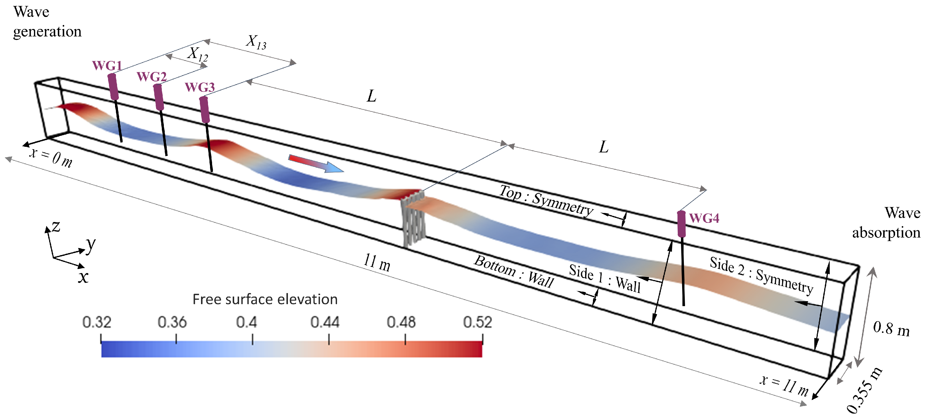
The performance of CPHB is numerically investigated by simulating the structure in a numerical wave tank (NWT). The numerical setup is similar to the setup from the experiments. The dimensions of the NWT are smaller than those of the physical wave tank to reduce the computational domain. The length of the NWT is 11 m based on the minimum requirement to compute Kt and Kr as per Isaacson [32] and Mansard and Funke [51]. The width of the tank is truncated by half (0.71 m to 0.355 m) using the symmetric plane boundary condition applied on one side of the tank. The other side of the tank has a no-slip wall boundary condition. Similar boundary conditions are also applied at the bottom of the tank. The waves are generated at one end using the Dirichlet inlet boundary condition. The active absorption method is adopted at the opposite end to absorb the transmitted waves, requiring no additional tank length. At the top of the NWT, a symmetric plane boundary condition is applied to represent the tank being open to the atmosphere. The potential effects of re-reflection in the NWT may be at the very minimum and not cognisable such that they may not have a noticeable effect on the results [52]. The details of the boundary conditions of NWT are presented in Figure 4. The same scale as that of the physical model (1:30) is adopted in the numerical model. In the case of monochromatic waves, the waves are reconstructed using the free surface elevation data measured by WG5 (refer to Figure 2).
In REEF3D, the free surface elevation is calculated using numerical wave gauges. The Kr for monochromatic waves is calculated using the three-probe approach in order to ensure consistency between physical and numerical modelling. The positioning of wave gauges is in accordance with the physical modelling (X12 = L/3 and X13 = 2L/3) as shown in Figure 4. For monochromatic waves, the Kt, Kr and Kd are calculated as per Equations (7)–(9), respectively.
where Hi represents the incident wave height, and Ht and Hr represent the transmitted and reflected wave heights, respectively. The dissipation coefficient Kd is computed using the wave energy conservation formula.
However, because the three-probe approach is confined to monochromatic waves, the Mansard and Funke [51] methodology is employed for irregular waves to separate the partial standing waves into incident and reflected wave components, (Hi and Hr, respectively). WG3 is positioned at a distance of L towards the seaside of the structure. WG1 and WG2 are separated by X12 = L/10. The distance between WG1 and WG3 is constrained to lie within the ranges of L/6 < X13 < L/3, X13 ≠ L/5 and X13≠ 3L/10. Hence, X13 = L/4 is selected to adhere to these limitations. The transmitted wave height is measured using WG4, which is positioned at a distance of L, as shown in Figure 2.
The wave climate conditions considered in the study area (Mangaluru Coast, west coast of India) are satisfactorily represented by the Scott–Wiegel spectra [53,54,55,56]. Therefore, the present study chooses the Scott–Wiegel spectrum [57] to generate the irregular waves (refer to Equation (10)). The Scott–Wiegel spectrum is expressed in terms of significant incident wave height as given below:
where S(ω) is the spectral energy at angular wave frequency , and ωp is the peak angular wave frequency. The wave surface elevation data are generated theoretically for the required His and Tp by employing the equation of the Scott–Wiegel spectrum. Using the theoretical time-domain data, the waves are reconstructed in the NWT. The waves are simulated for a duration of 120 s. The wave transmission coefficient is calculated as Kt = Hts/His. The significant incident wave height (His) and significant transmitted wave height (Hts) are obtained using a frequency domain analysis. The significant incident wave height is estimated as His = 4.0, where m0i is the zeroth moment of the incident wave spectrum obtained using the numerical probe located at x = 0.02 m. Similarly, the significant transmitted wave height is calculated using Hts = 4.0, where m0t is the zeroth moment of the transmitted wave spectrum obtained using Wave Probe 4. The reflection coefficient (Kr) is estimated using the procedure proposed by Mansard and Funke [51]. The dissipation coefficient (Kd) is calculated using Equation (9), which is derived based on the law of conservation of wave energy.
3. Results and Discussion
Before carrying out simulations with a CPHB, the quality of the generated waves is examined with different grid sizes and CFL numbers to determine their optimal values for the current study. The numerical results for non-perforated and perforated CPHBs with monochromatic waves are validated by comparison with the experimental data described in Section 2.1. The best-performing non-perforated and perforated CPHB models are further investigated with irregular waves.
3.1. Validation of Wave Generation
Validation of the reconstructed waves is carried out in a two-dimensional (2D) NWT at a water depth of 0.4 m without including the structure. Since the reconstructed waves are unidirectional, the validation study is conducted in a 2D NWT. The 2D tank is modelled with symmetric boundary conditions on both side planes. No turbulence modelling is used for simulations in the numerical wave tank without structures. To evaluate the accuracy of the free surface data, the experimental and numerical profiles for different grid sizes and CFL numbers are compared. Numerical simulations with finer grid sizes and smaller CFL numbers result in more accurate results, although with higher computational time.
3.1.1. Monochromatic Waves
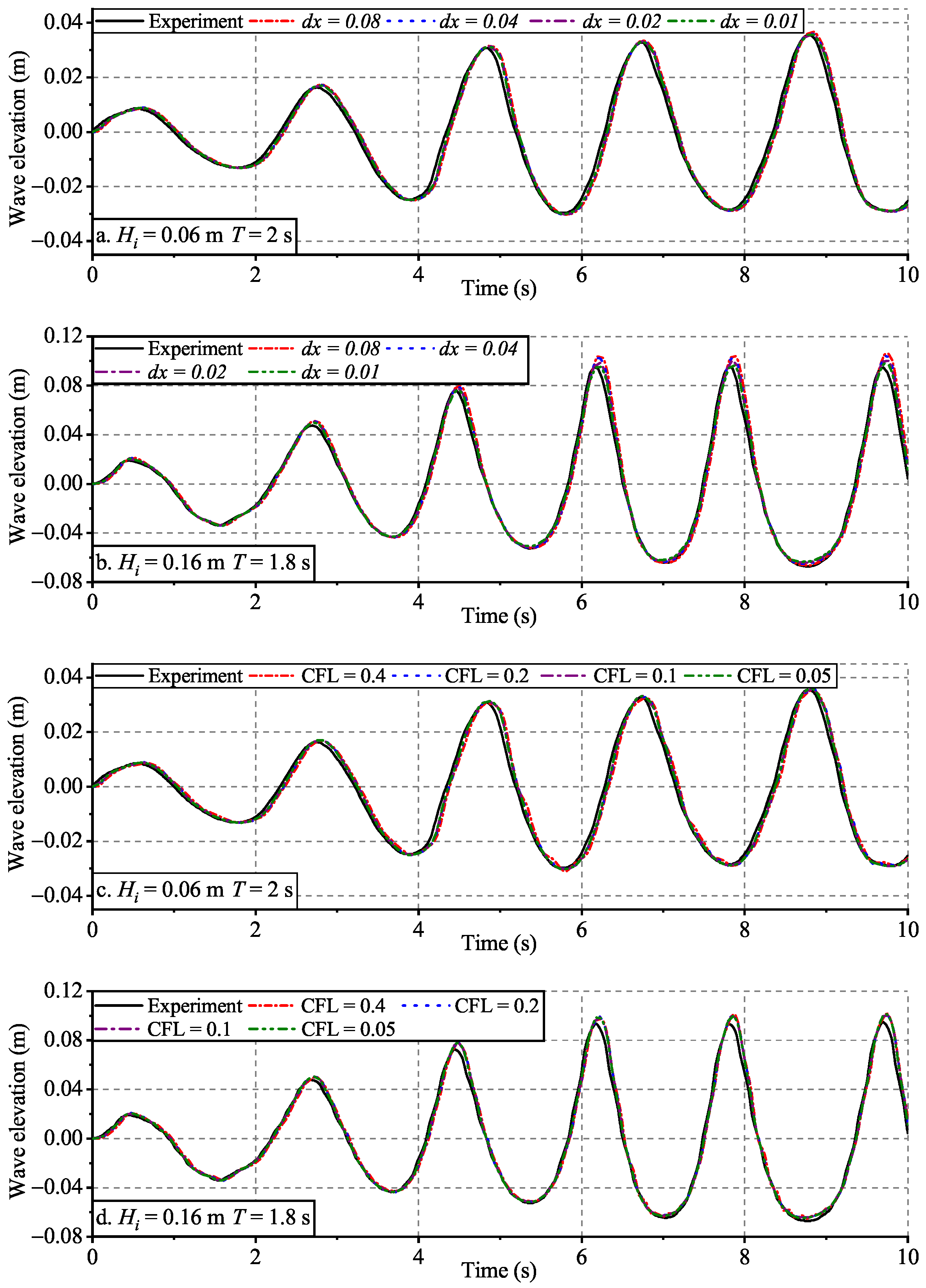
To maintain similitude between physical and numerical modelling, the time-series data from the experiments are used to generate the same waves in NWT. The quality of wave generation is verified for steeper (Hi = 0.16 m, T = 1.8 s) and gentler (Hi = 0.06 m, T = 2.0 s) wave heights for various grid sizes, as shown in Figure 5. For grid size optimisation, uniform grid sizes dx = dy = dz = 0.08 m, 0.04 m, 0.02 m or 0.01 m are considered while keeping the CFL number constant at 0.1. Table 2 presents the root-mean-square error (RMSE) values obtained by comparing the experimental data with the numerically reconstructed wave surface elevation. The grid size analysis clearly shows that lowering the grid size from 0.08 m to 0.04 m results in a reduction in the RMSE values. The free surface elevation is found to agree well with the measured data for a grid size of 0.02 m. Further reducing the grid size from 0.02 to 0.01 m shows a negligible improvement with higher computational time. It can be concluded from the grid refinement study that a grid size of 0.02 m is sufficient for accurate wave generation with a maximum RMSE of 0.0053 m. Therefore, dx= 0.02 m is used for further investigation of the influence of CFL number on wave generation. The CFL numbers considered for the sensitivity study are 0.4, 0.2, 0.1 and 0.05, as shown in Figure 5, and the errors associated are listed in Table 2.
Similar to the grid refinement study, a CFL number of 0.1 appears to be optimal: an increase improves the wave quality, whereas a reduction shows negligible improvement and with higher computational time. From the above sensitivity study on grid size and CFL number, it is clear that simulating the waves with a CFL number of 0.1 with a grid size less than or equal to 0.02 m results in an accurate representation of the free surface elevation. The computed RMSE values of the reconstructed waves are reasonable. Further, it is essential to ensure that the quality of wave generation in 2D (11 m × 0.02 m × 0.8 m) and 3D (11 m × 0.355 m × 0.8 m) NWTs is consistent. Hence, a simulation is run in a 3D NWT for the Hi = 0.16 m and T = 1.8 s case by employing the optimum grid size and CFL number (dx = 0.02 m and CFL = 0.1). It is found that the free surface elevations calculated in the 2D and the 3D NWT are in agreement.
3.1.2. Irregular Waves
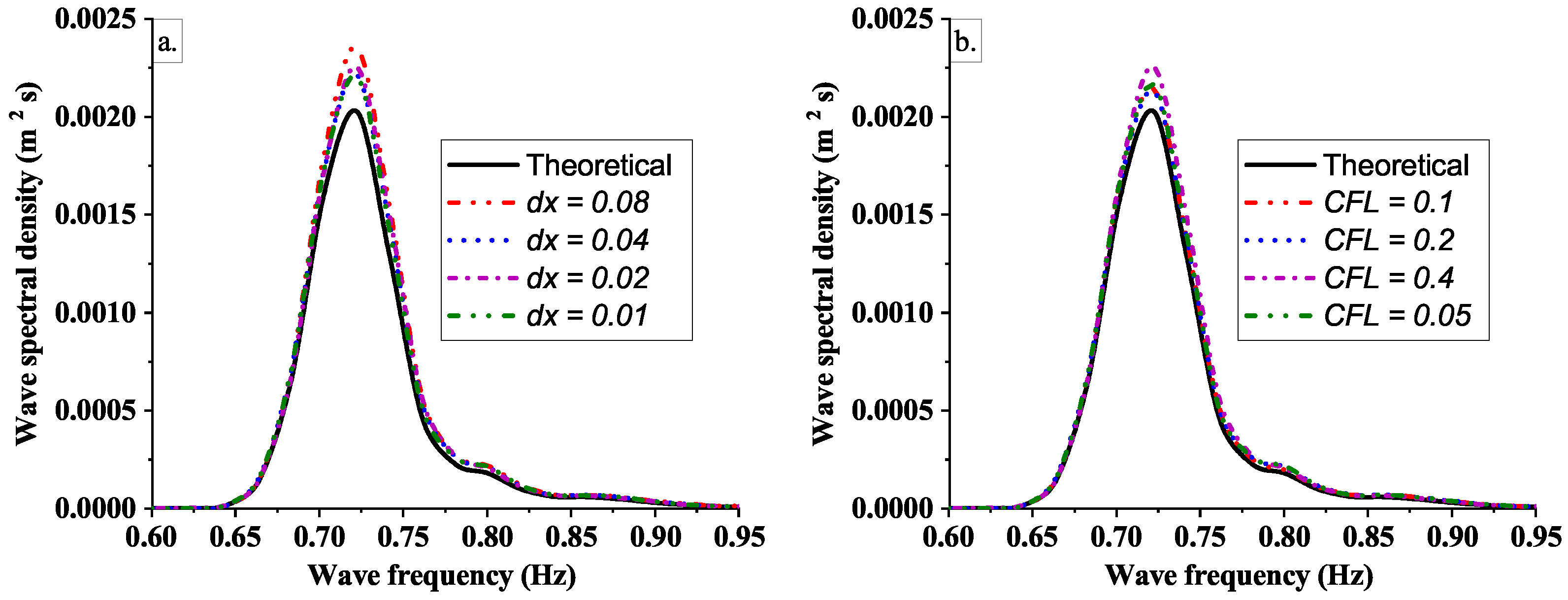
The quality of the reconstructed irregular wave profile and free surface elevation spectra are evaluated with different grid sizes and CFL numbers for the steeper wave: (His = 0.12 m and Tp = 1.4 s). Similar to monochromatic waves, the simulations are performed in a 2D NWT by considering uniform grid sizes of 0.08 m, 0.04 m, 0.02 m or 0.01 m while maintaining CFL= 0.1. The free surface elevation is measured in the NWT using the numerical wave probe at x = 0.02 m. Figure 6a represents the spectral wave density obtained for different grid sizes. The numerical peak spectral wave density is higher than the experimental peak spectral wave density by 15.82% and 10.76% for grid sizes of 0.08 m and 0.04 m, respectively. The difference between the numerical and experimental peak spectral wave density decreases to 9.34% when the grid size is reduced to 0.02 m. Further reduction in grid size from 0.02 m to 0.01 m resulted in a reduction in error of only 0.38% (9.34% to 8.95%). Since the improvement of results is negligible between grid sizes of 0.02 m and 0.01 m, a grid size of 0.02 m is fixed for determining the optimum CFL number.
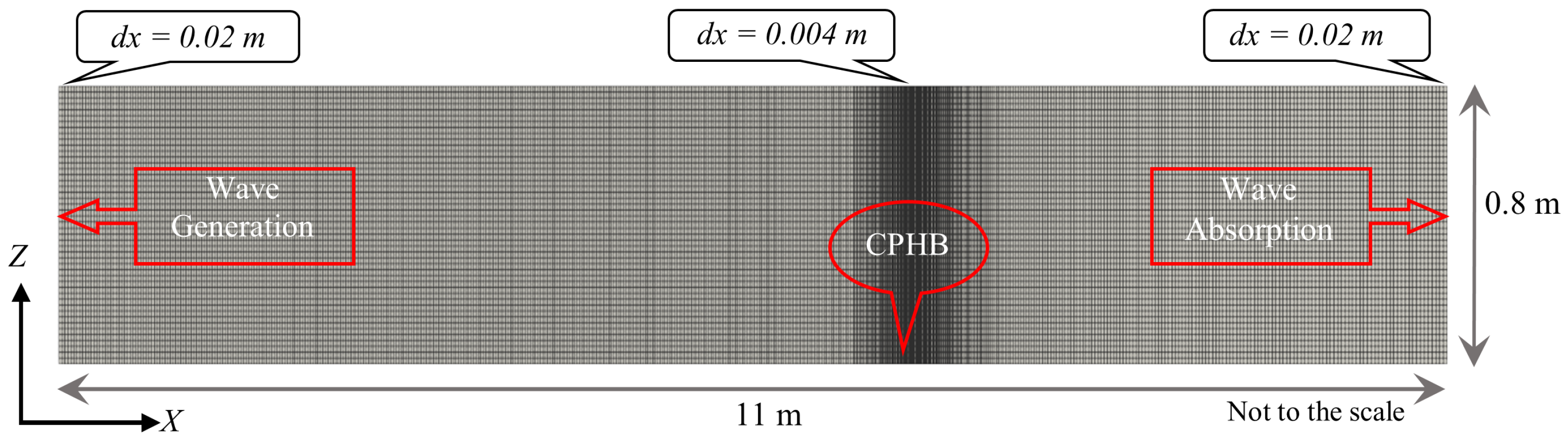
While simulating the CPHB, a non-uniform grid distribution based on a Cartesian system is adopted in the present work to reduce computational effort. In the x-direction, a coarser grid size of 0.02 m is maintained at the generation and absorption zone. In the numerical simulations, a grid with a size of 0.004 m is employed to accurately characterize the CPHB structure. The grid sizes are varied gradually from 0.02 m to 0.004 by employing a sine-based stretching function (refer to Figure 7). At the same time, a uniform grid size of 0.004 m is adopted in both the y- and z-directions. Using these non-uniform grids (refer to Figure 7), a without-structure simulation is performed in 2D NWT to assess the reliability of wave generation. The free surface elevations of the 2D uniform grid and 2D non-uniform grid are seen to be in harmony. Therefore, it can be concluded that the accuracy of wave generation is unaffected by the non-uniform grid distribution adopted for the 3D NWT simulations.
3.2. Performance of CPHB with Monochromatic Waves
Initially, simulations of non-perforated and perforated CPHBs with monochromatic waves are performed. The influence of pile head diameter on non-perforated CPHBs is investigated using two different pile head diameters (D/Hmax = 0.4 and 0.5). Perforations with the optimum size and arrangement (Pa = 50%, P = 19.2%, and S/D = 0.25) indicated by Sathyanarayana et al. [28] are used for the perforated structure. The results of the non-perforated and perforated CPHBs are validated with the experimental data and analysed to arrive at the best-performing configuration of CPHBs. The study is carried out in various wave energy regions with intermediate water depth conditions. The different combinations of wave heights and periods considered for the simulation of monochromatic waves are listed in Table 3. The cases are selected such that the wave steepnesses (Hi/gT2) are of the same range as those in the experiments. Finally, The CPHBs with the best-performing configuration with and without perforations are subjected to irregular wave conditions.
3.2.1. Validation of Numerical Results with Experimental Data
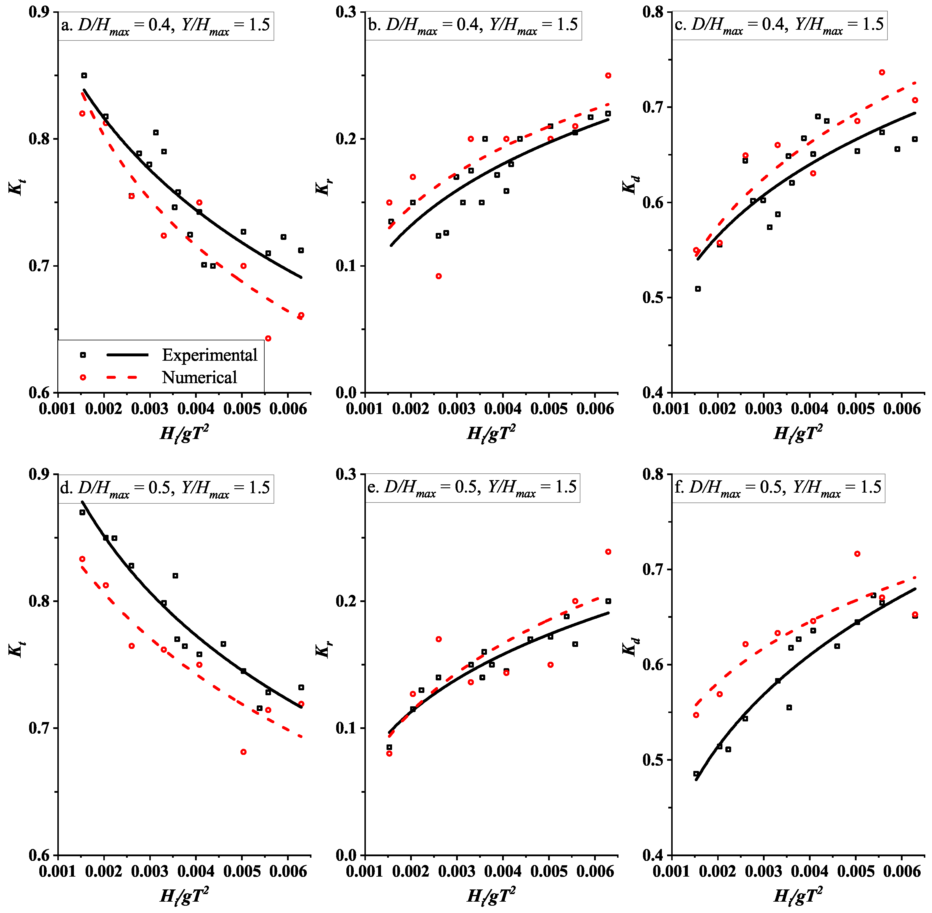
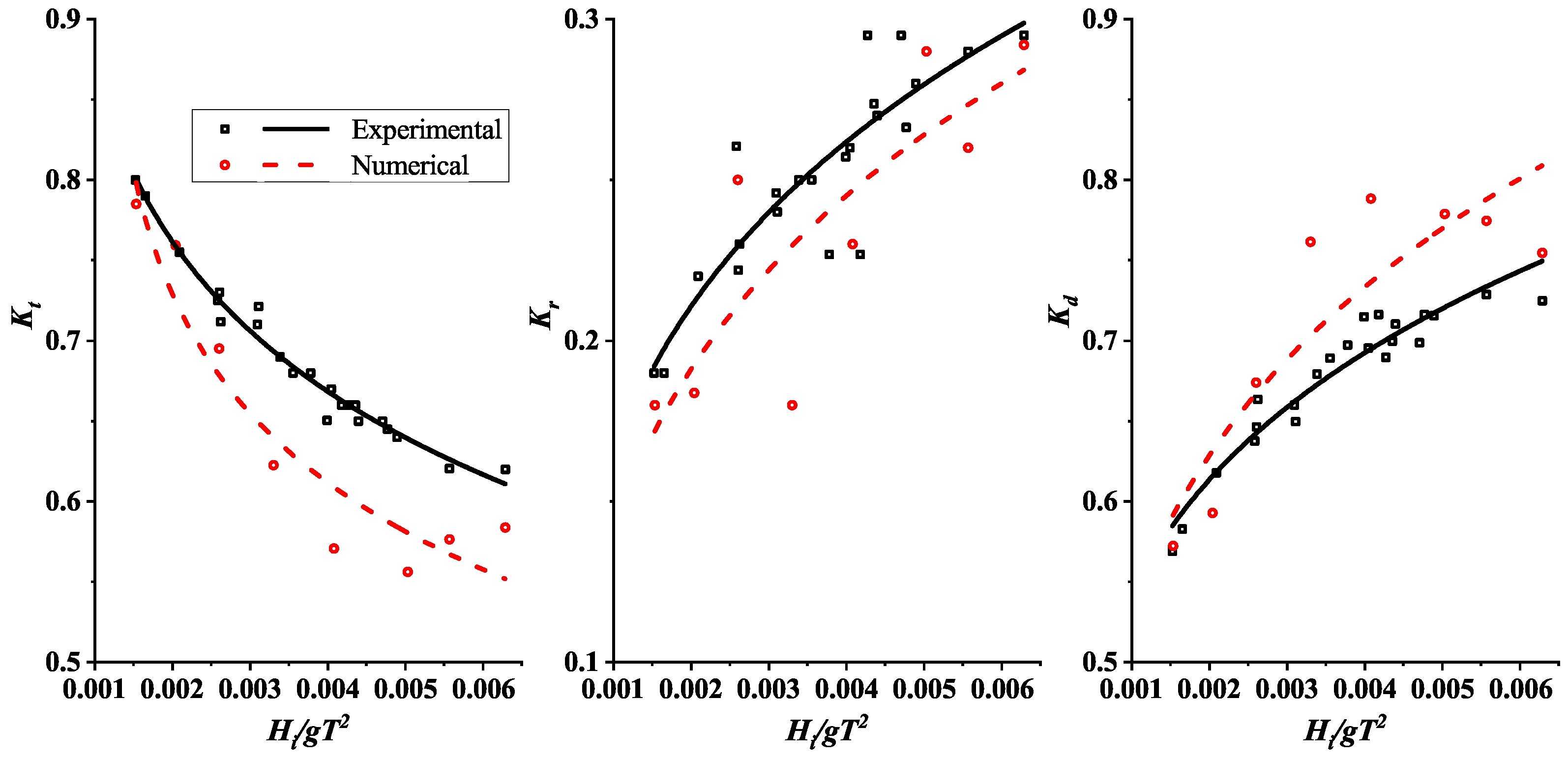
The Kt, Kr and Kd of two non-perforated pile heads (D/Hmax = 0.4 and 0.5) are compared to experimental data [27] in Figure 8. Figure 9 presents the validation of numerical results with the experimental data for the case of the perforated CPHB. Best-fit lines are drawn to gain a better understanding and interpretation of the results. The trend lines plotted for the numerical results of both non-perforated and perforated CPHBs match with those of the experimental results to a reasonable extent. In the case of non-perforated CPHBs, the numerical results slightly under-predict for Kt (less than 4%) and over-predict for Kr and Kd (less than 9%) for both cases of D/Hmax. For the perforated CPHB, the variation is slightly higher (up to 12%) compared to the non-perforated structure. The RMSE calculated by comparing the experimental and numerical results is summarised in Table 4. The comparison of results shows that the numerically determined performance characteristics of both non-perforated and perforated CPHBs are in relatively good agreement with the experimental data.
3.2.2. Effect of Relative Pile Head Diameter
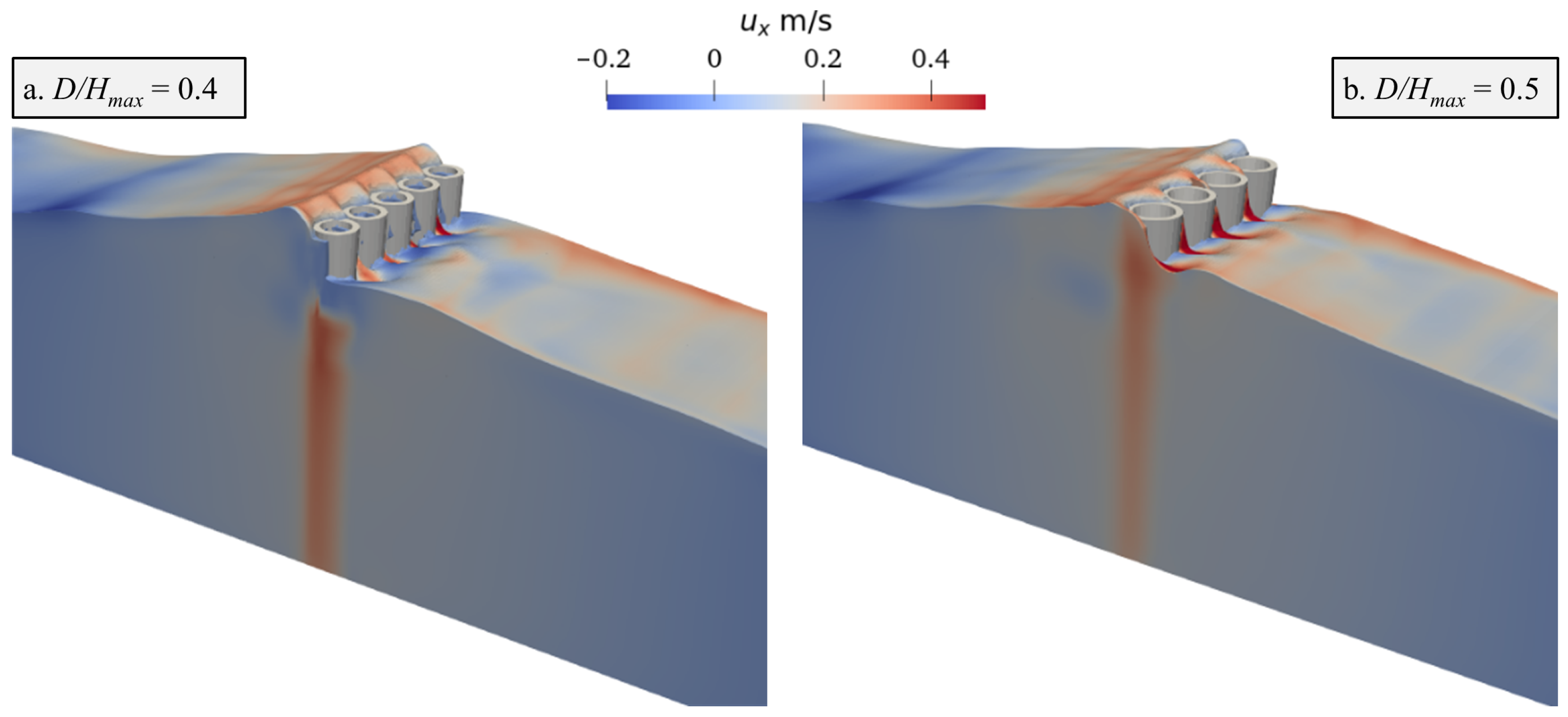
Simulations of two different diameters (D/Hmax = 0.4 and 0.5) of non-perforated CPHBs are performed to determine the influence of the pile head diameter and to arrive at the optimum-performing configuration. Figure 10 presents the simulated images of the wave crest interaction with non-perforated CPHBs for various D/Hmax at the same time step (t = 9.10 s). Due to the larger numbers and smaller spacing of pile heads, the horizontal velocity of waves (ux) is obstructed to a significant amount in the case of D/Hmax = 0.4 compared to that of D/Hmax= 0.5 (refer to Figure 10). To overcome the obstruction, a relatively considerable number of waves may enter into the hollow portion of the pile head for D/Hmax = 0.4 compared to D/Hmax = 0.5. The water that enters the perforated pile head flushes out and results in additional energy loss, as demonstrated in Figure 10a. When D/Hmax = 0.5, a relatively higher quantity of waves are transmitted between the pile heads with an intensified velocity, as seen in Figure 10b. The CPHB with D/Hmax = 0.4 configuration has a higher number of piles and about 9.8% higher blockage area compared to D/Hmax = 0.5. The higher blockage area increases the effectiveness of the obstruction of wave energy, leading to wave breaking over the structure along with higher wave reflection.
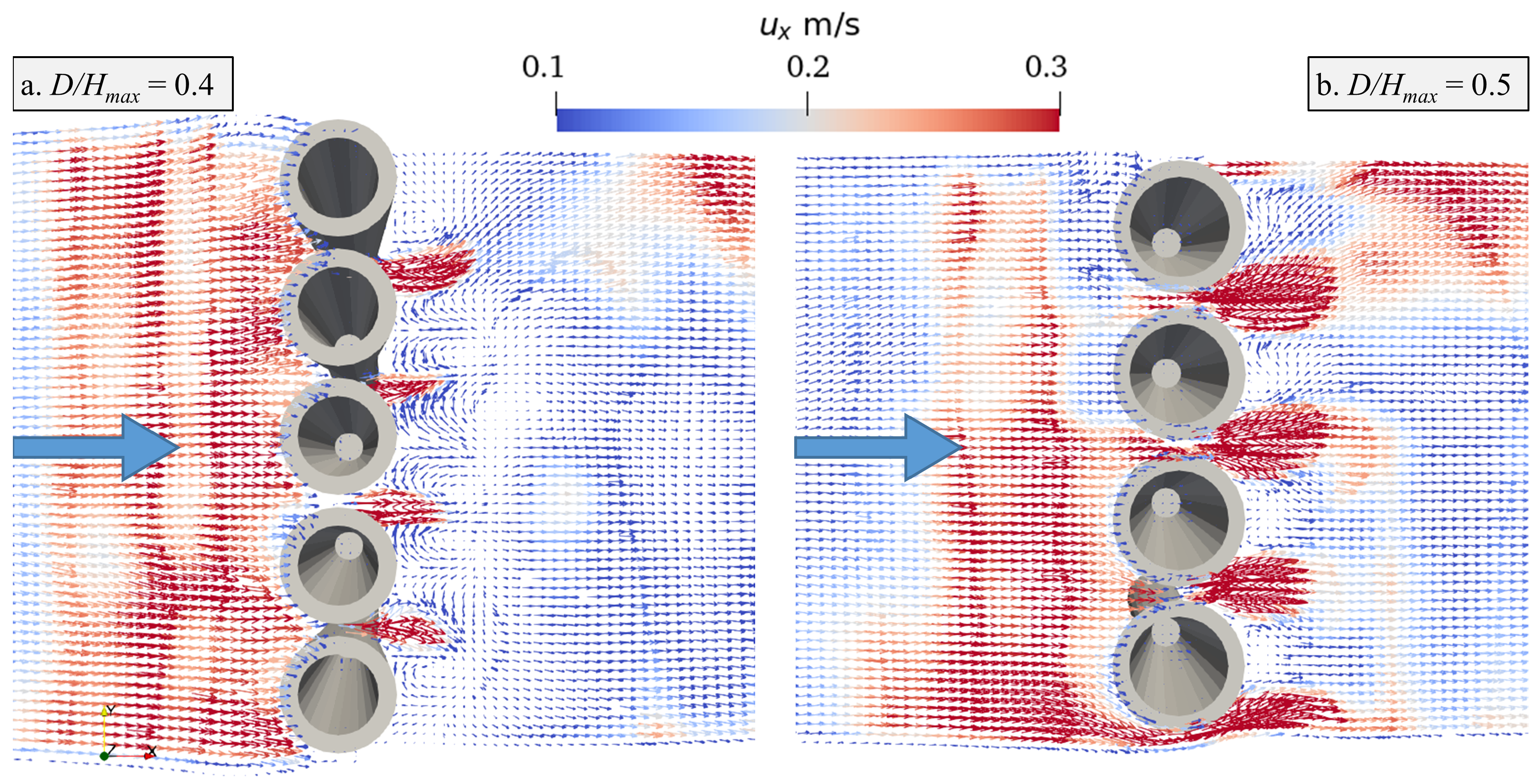
The plan-view of the particle path lines during the propagation of the wave crest over the non-perforated pile head is presented in Figure 11. When D/Hmax = 0.4, the horizontal propagation of the incident wave at the free surface is obstructed by the structure to a substantial extent, whereas, for D/Hmax = 0.5, the wave easily propagates through the larger gaps without a significant reduction in velocity. In addition, the formation of vortices is clearly noticed on the lee side of the structure for D/Hmax = 0.4 (Figure 11a), which contributes to energy losses. When D/Hmax = 0.5, the energy dissipation through vortex formation is reduced, possibly due to lower blockage resulting from a long distance between the pile heads.
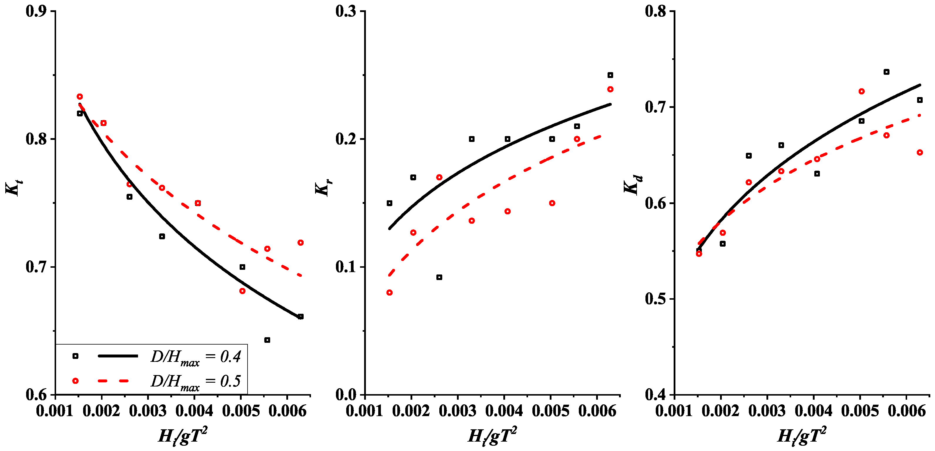
The wave attenuation characteristics determined by numerical modelling are compared in Figure 12 to examine the influence of pile head diameter (D/Hmax). For higher wave steepness, D/Hmax = 0.4 exhibits about 8% lower Kt, 18.2% higher Kr and 6% higher Kd compared to D/Hmax = 0.5. At lower wave steepness, it is noticed that the Kt and Kd are comparable. The lowest Kt of 0.64 is obtained for D/Hmax = 0.4 at a higher wave steepness along with Kr of 0.22 and Kd of 0.73.
3.2.3. Effect of Perforations
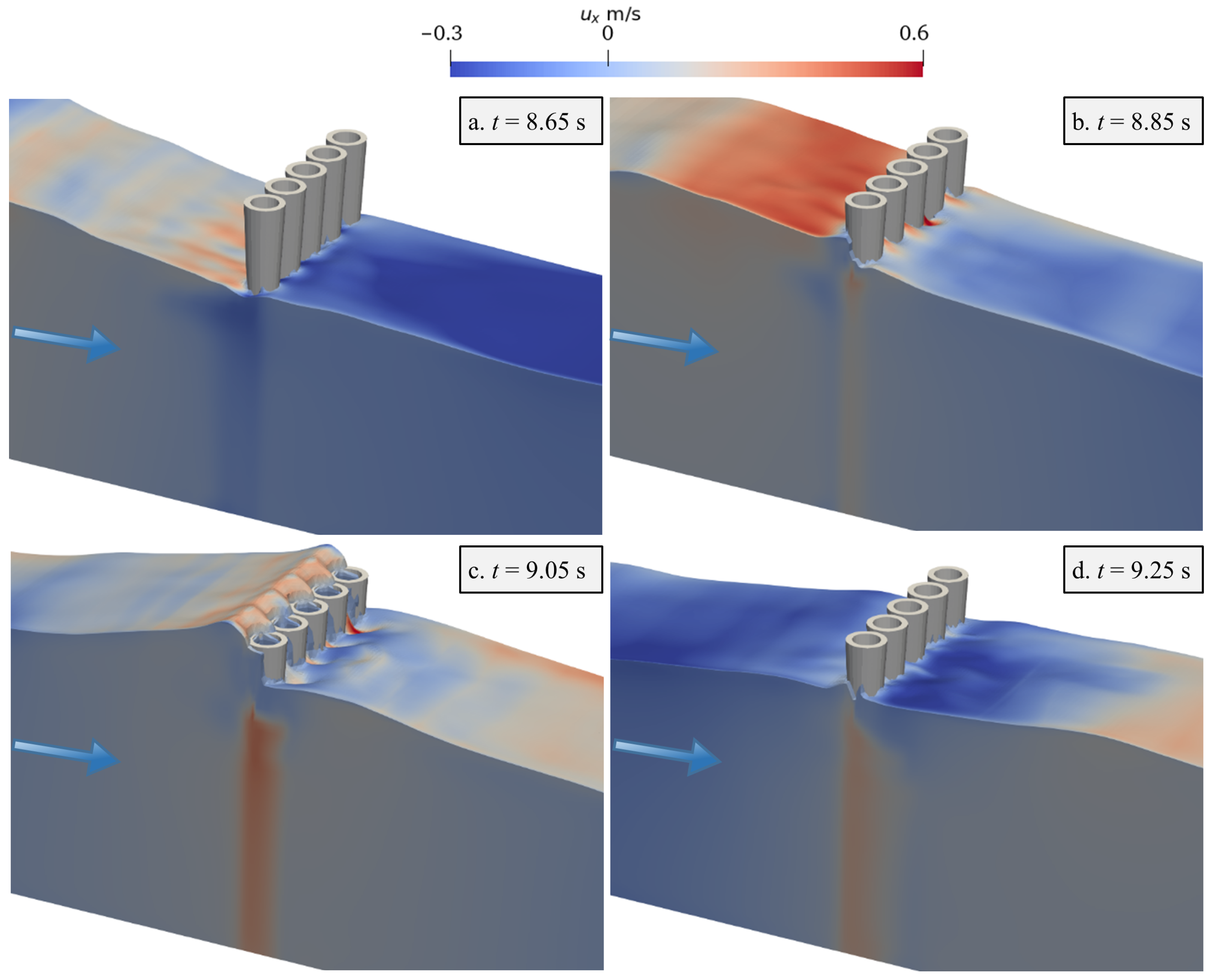
The key factors responsible for pile breakwater’s wave attenuation are inertial resistance, contraction, vortex shedding and wave reflection. The idea behind providing a higher obstruction area near the free surface is to distort the orbital motion of the waves, which is maximal at the free surface. Figure 13 clearly demonstrates the changes in the horizontal component of the orbital velocity (ux) as the wave interacts with the non-perforated CPHBs at different time instances (t). The increased area of the piles (CPHBs) contributes to a comparatively higher obstruction than conventional pile breakwaters, due to which the horizontal velocity of the waves is obstructed (refer to Figure 13b). Due to this obstruction, a part of the wave may propagate through the gaps between pile heads with an intensified velocity. Another part may flow over the pile head and enter the hollow portion of CPH (refer to Figure 13c). This results in turbulence and energy dissipation along with partial reflection of waves, as presented in Figure 13c.
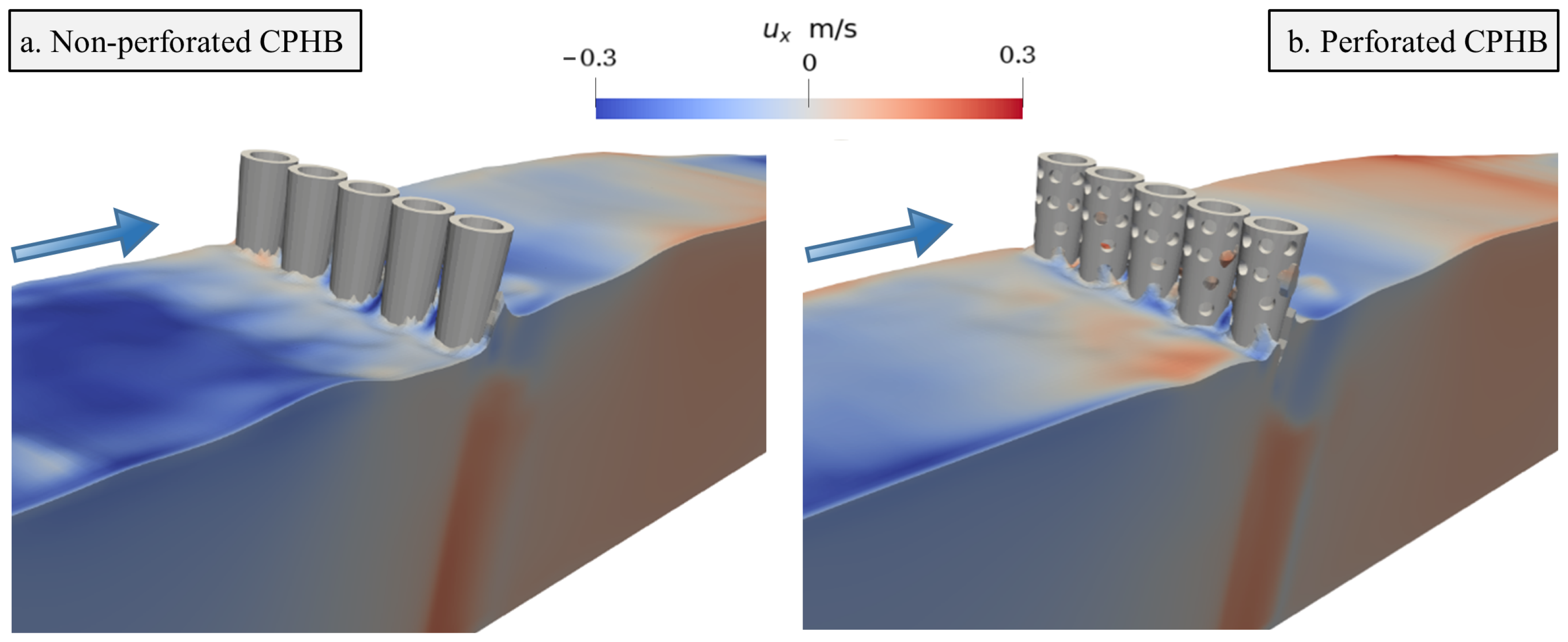
The gentler waves flow around the CPHB structure without entering the hollow part of the CPH. Therefore, to increase the wave–structure interaction, perforations are incorporated on the seaside surface of the CPH so that the waves, irrespective of their steepness, enter the hollow portion of the pile head. Under wave trough incidence, the water that enters during crest incidence flows back through the perforations and confronts the following incident wave crest, creating a disturbance on the seaside of the structure. The optimum configuration of perforations (Pa = 50%, S/D = 0.25 and P =19.2%) from Sathyanarayana et al. [28] is used in the present study. Figure 14 compares the changes in the horizontal velocity during the wave trough’s interaction with the non-perforated and perforated CPHBs. It is noticed (refer to Figure 14a,b) that water that entered the CPHB flows out of perforations, causing comparatively higher reflection and increased turbulence on the seaside of the structure compared to the non-perforated structure.
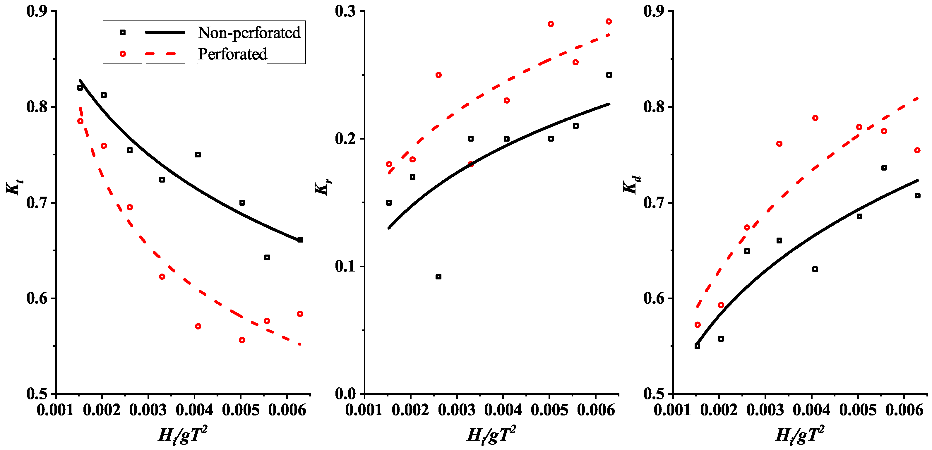
The performance characteristics of non-perforated and perforated CPHBs are compared in Figure 15 to determine the influence of the perforations. Introducing perforations on the CPHs reduces Kt by about 5% to 16.5%. The values of Kr and Kd are increased by about 27.25% and 10.28% on average, respectively. A minimum Kt of 0.54 is calculated for the perforated CPHB at higher wave steepness, associated with a Kr and Kd of 0.28 and 0.80, respectively. The observed performances of the non-perforated and perforated CPHBs are in agreement with the experimental data [28] and other similar studies on pile breakwaters [21,22,24,26].
3.2.4. Effect of Wave Steepness
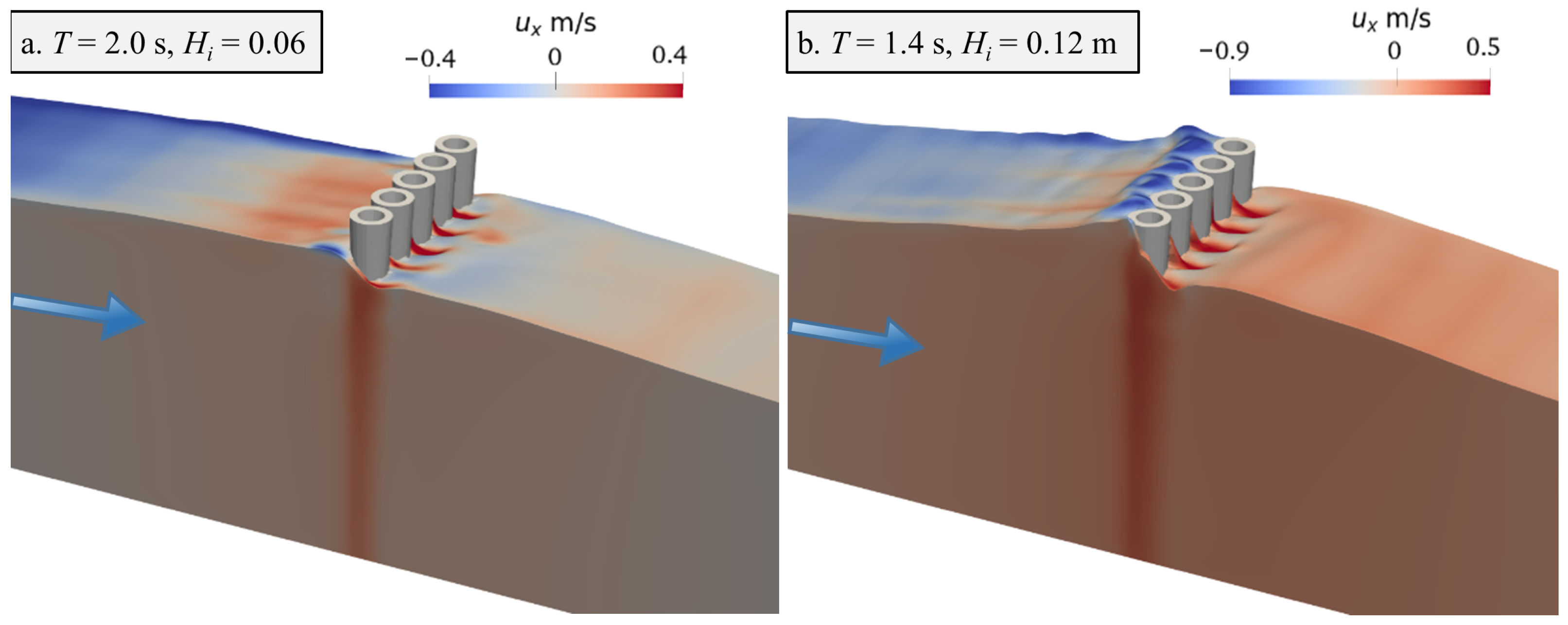
The wave steepness parameter (Hi/gT2) accounts for both the effects of wave height and period. Steeper waves tend to be unstable in nature, and the slightest obstruction to their propagation triggers wave breaking and energy loss, while gentler waves are comparatively stable. Figure 16 presents the wave interaction with the steeper and gentler waves, in which the steeper wave and gentler wave correspond to cases M1 and M8, respectively (refer to Table 3). As noticed in Figure 16, turbulence generation is higher for M1 than M8, which results in higher energy losses and higher wave attenuation. In the case of M8, the wave energy transmits smoothly around the pile heads without losing much energy, leading to higher Kt values. In addition, higher reflection is calculated for the M1 case than for M8, as illustrated in Figure 16. In general, it can be inferred from Figure 8 and Figure 9 that Kt is indirectly proportional to the wave steepness, while Kr and Kd are directly proportional. The wave attenuation capability of the CPHB is more pronounced for steeper incident waves than for gentler waves for both non-perforated and perforated CPHBs. For the non-perforated CPHB (D/Hmax = 0.4), the value of Kt obtained against steeper waves is about 22% smaller than that of gentler waves. Similarly, for the same CPHB configuration with perforations, about a 23.6% smaller Kt is obtained.
In the present study, the CPHB structure is tested considering the wave climate off the Mangaluru Coast. From the test results, the structure appears to be more efficient in wave attenuation against steep waves than gentle waves with increased energy dissipation. Further, if the structure is tested for a wider range of wave periods, the structure performance is expected to be better with smaller transmission and higher energy dissipation when subjected to steep waves (T < 1.4 s), whereas gentle waves (T > 2 s) are expected to propagate with the least interaction at the pile structure, thus indicating increased wave transmission and the smallest energy dissipation.
From both the experimental and numerical studies, it is evident that the non-perforated CPHB with D/Hmax = 0.4 performs better than D/Hmax = 0.5. Further, perforations on the CPH surface proved to be advantageous in enhancing CPHB wave attenuation characteristics. Therefore, the best-performing non-perforated CPHB (D/Hmax = 0.4, Y/Hmax = 1.5 and b/D = 0.1) and perforated CPHB (Pa = 50%, P = 19.2% and S/D = 0.25) are considered for further investigation with irregular waves.
3.2.5. Performance Comparison with Other Pile Breakwater Structures
In order to understand the possible benefits of CPHB over other similar pile breakwater structures, the performances are compared and listed in Table 5. The optimally configured non-perforated and perforated CPHBs with monochromatic waves are considered for the comparison study. The results of the present study are compared with non-perforated and perforated hollow pile breakwaters [24,26], non-perforated and perforated suspended pipe breakwaters [23,25], rectangular pile breakwaters [58] and zigzag porous screen breakwaters [59]. It is found that the wave attenuation characteristics of the CPHB structure are in line with the other structures with a minimal number of pile units. The number of CPHB units per meter length is about 45.3% less than both hollow pile breakwaters and suspended pipe breakwaters, 74.8% less than rectangular pile breakwaters and 30.7% less than zigzag porous screen breakwaters. Overall, the comparison demonstrated that the CPHB structure is a better wave attenuator than the other structures considered in the comparison.
3.3. Comparison of CPHB Performance with Monochromatic and Irregular Waves
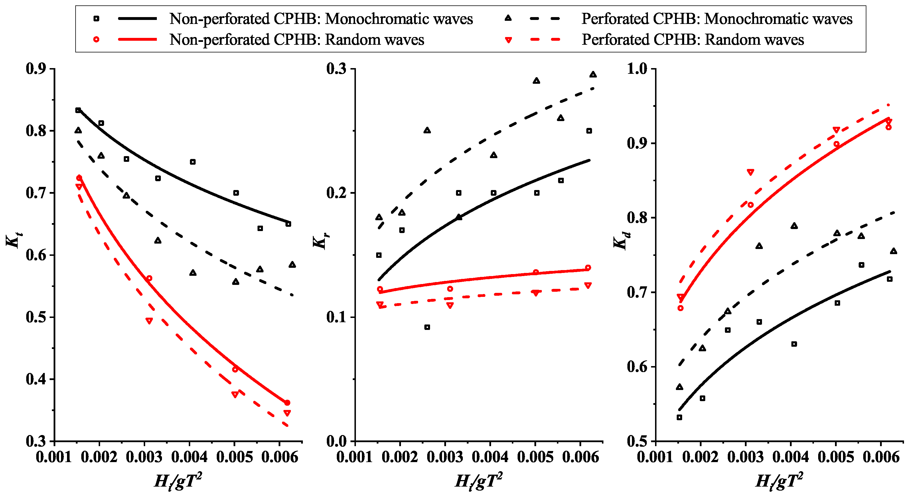
The hydraulic performance of the CPHB structure is studied with irregular waves by employing the Scott–Wiegel spectrum. The investigation is carried out only for the best-performing non-perforated (D/Hmax = 0.4, Y/Hmax = 1.5 and b/D = 0.1) and perforated CPHBs Pa = 50%, (P = 19.2% and S/D = 0.25) obtained against monochromatic waves. The combination of significant incident wave height (His) and peak wave period (Tp) is selected to match the experimental wave steepness range with uniform distribution. The Tp and His values considered in the study are listed in Table 6. Figure 17 presents the comparison of performance characteristics between monochromatic and irregular waves for both non-perforated and perforated CPHBs. The trend lines are drawn for the discrete data in order to clearly comprehend CPHB performance, and the results are then evaluated using the trend lines. A close examination of Figure 17 reveals that the trend of Kt, Kr and Kd with respect to wave steepness is similar to that seen for monochromatic waves.
The wave attenuation characteristics of the CPHBs are found to be better with irregular waves than monochromatic waves. The Kt values obtained for the non-perforated CPHBs with monochromatic wave test conditions range from 0.83 to 0.64, whereas for irregular waves, the range is between 0.72 and 0.36. Similarly, for the perforated CPHBs, the Kt varied from 0.8 to 0.54 with monochromatic waves and 0.68 to 0.33 in the case of irregular waves. It is observed that the Kr obtained for the irregular waves is lower than that of the monochromatic waves for both the non-perforated and perforated CPHBs. Additionally, the dissipation characteristics are higher for both cases (non-perforated and perforated) of CPHBs with irregular waves. Therefore, it can be stated that the performance characteristics calculated using the monochromatic wave conditions are conservative. Similar deviations in the performance characteristics between monochromatic and irregular waves have been reported in the literature for other pile structures, including partially immersed twin vertical barriers [60], T-type breakwaters [61] and ⊥-type breakwaters [62]. Overall, it is evident that the non-perforated CPHB with the structural configuration of max = 0.4, max = 1.5 and = 0.1 can attenuate waves up to 67% with irregular wave conditions. Incorporating the perforations enhances the wave attenuation capability of the structure by about 5% to 10% with irregular wave climates.
4. Conclusions
Numerical investigation of the performance characteristics of conical pile head breakwaters is carried out using the open-source CFD tool REEF3D with monochromatic and irregular waves. The following conclusions are drawn from the analysis of the results.
- (1)
- In general, Kt is found to be indirectly proportional to the wave steepness, whereas Kr and Kd exhibit the opposite pattern.
- (2)
- Validation of the numerical results with the experimental data shows that REEF3D produces reliable results with acceptable RMSE values.
- (3)
- The hydraulic performance of the CPHB structure is found to be more conservative with monochromatic waves than with irregular waves.
- (4)
- In the case of irregular waves, Kt ranges from 0.72 to 0.36 for the non-perforated CPHB with an optimum configuration of D/ = 0.4, = 1.5 and = 0.1. For the same configuration, Kt ranges between 0.83 and 0.64 with monochromatic waves.
- (5)
- Introducing perforations with the optimum configuration ( = 50%, = 0.25 and P = 19.2%) on the CPHs enhanced the transmission capability of the CPHB by about 5% to 16.5% with monochromatic waves and 5% to 10% with irregular waves.
Overall, the numerical model of the CPHB mimics the physical phenomenon of experimental studies, and the perforated CPHB with the proposed configuration is capable of reducing the wave transmission up to 67% with irregular waves. Hence, taking the site characteristics into consideration, the CPHB may be suitable for coastal protection where partial wave protection is adequate.
Author Contributions
Conceptualization, A.H.S., P.U. and K.G.S.; Investigation, A.H.S. and P.S.S.; Methodology, A.H.S., P.S.S. and K.G.S.; Formal analysis, A.H.S.; Funding acquisition, P.U.; Resources, P.U., A.K. and H.B.; Software, H.B.; Supervision, P.U., K.G.S. and A.K.; Validation, A.H.S. and P.S.S.; Visualization, A.H.S.; Writing—original draft, A.H.S.; Writing—review and editing, P.U., K.G.S., H.B. and A.K. All authors have read and agreed to the published version of the manuscript.
Funding
The Ministry of Education (MoE), Government of India, supported this research work through the SPARC initiative under the project “Environmental innocuous pile head breakwater for the mitigation of coastal erosion” (Project ID. 262).
Data Availability Statement
All relevant data are included in the article.
Acknowledgments
The authors gratefully acknowledge the computational resources provided by NTNU, Norway, by the National Research Infrastructure Service (NRIS) under project number: NN2620K.
Conflicts of Interest
The authors declare no conflict of interest. The founding sponsors had no role in the design of the study; in the collection, analyses, or interpretation of data; in the writing of the manuscript, and in the decision to publish the results.
References
- Zhu, D.T.; Xie, Y.F. Hydrodynamic characteristics of offshore and pile breakwaters. Ocean Eng. 2015, 104, 257–265. [Google Scholar] [CrossRef]
- Gao, J.; He, Z.; Huang, X.; Liu, Q.; Zang, J.; Wang, G. Effects of free heave motion on wave resonance inside a narrow gap between two boxes under wave actions. Ocean Eng. 2021, 224, 108753. [Google Scholar] [CrossRef]
- Gao, J.; Ma, X.; Dong, G.; Chen, H.; Liu, Q.; Zang, J. Investigation on the effects of Bragg reflection on harbor oscillations. Coast. Eng. 2021, 170, 103977. [Google Scholar] [CrossRef]
- Herbich, J.B.; Douglas, B. Wave transmission through a double-row pile breakwater. In Proceedings of the 21st Coastal Engineering Conference, Costa del Sol-Malaga, Spain, 20–25 June 1988; pp. 2229–2241. [Google Scholar]
- Hutchinson, P.; Raudkivi, A. Case history of a spaced pile breakwater at Half Moon Bay Marina Auckland, New Zealand. In Proceedings of the 19th International Conference on Coastal Engineering, Houston, TX, USA, 3–7 September 1984; Volume 84, pp. 2530–2533. [Google Scholar]
- Koraim, A.; Salem, T. The hydrodynamic characteristics of a single suspended row of half pipes under regular waves. Ocean Eng. 1984 2012, 50, 1–9. [Google Scholar] [CrossRef]
- Jeya, T.J.; Sriram, V.; Sundar, V. Hydrodynamic characteristics of vertical and quadrant face pile supported breakwater under oblique waves. Proc. Inst. Mech. Eng. Part M J. Eng. Marit. Environ. 2022, 236, 62–73. [Google Scholar] [CrossRef]
- Yin, M.; Zhao, X.; Luo, M.; Sun, H. Flow pattern and hydrodynamic parameters of pile breakwater under solitary wave using OpenFOAM. Ocean Eng. 2021, 235, 109381. [Google Scholar] [CrossRef]
- Elsharnouby, B.; Soliman, A.; Elnaggar, M.; Elshahat, M. Study of environment friendly porous suspended breakwater for the Egyptian Northwestern Coast. Ocean Eng. 2012, 48, 47–58. [Google Scholar] [CrossRef]
- Liu, H.; Ghidaoui, M.S.; Huang, Z.; Yuan, Z.; Wang, J. Numerical investigation of the interactions between solitary waves and pile breakwaters using BGK-based methods. Comput. Math. Appl. 2011, 61, 3668–3677. [Google Scholar] [CrossRef] [Green Version]
- Park, W.S.; Kim, B.H.; Suh, K.D.; Lee, K.S. Scattering of irregular waves by vertical cylinders. Coast. Eng. J. 2000, 42, 253–271. [Google Scholar] [CrossRef] [Green Version]
- Suh, K.D.; Shin, S.; Cox, D.T. Hydrodynamic characteristics of pile-supported vertical wall breakwaters. J. Waterw. Port Coast. Ocean Eng. 2006, 132, 83–96. [Google Scholar] [CrossRef]
- Zhu, D. Hydrodynamic characteristics of a single-row pile breakwater. Coast. Eng. 2011, 58, 446–451. [Google Scholar] [CrossRef]
- Zhu, D.T. Full wave solution for hydrodynamic behaviors of pile breakwater. China Ocean Eng. 2013, 27, 323–334. [Google Scholar] [CrossRef]
- Van Weele, B.J.; Herbich, J.B. Wave reflection and transmission for pile arrays. In Proceedings of the 13th Conference on Coastal Engineering, Vancouver, BC, Canada, 10–14 July 1972; pp. 1935–1953. [Google Scholar]
- Ahmed, H.; Schlenkhoff, A. Numerical investigation of wave interaction with double vertical slotted walls. World Acad. Sci. Eng. Technol. Int. J. Environ. Ecol. Geol. Min. Eng. 2014, 8, 536–543. [Google Scholar]
- Koraim, A.; Iskander, M.; Elsayed, W. Hydrodynamic performance of double rows of piles suspending horizontal c shaped bars. Coast. Eng. 2014, 84, 81–96. [Google Scholar] [CrossRef]
- Ramnarayan, S.K.; Sannasiraj, S.; Sundar, V. Hydrodynamic characteristics of curved and vertical front face pile-supported breakwaters in regular waves. Ocean Eng. 2020, 216, 108105. [Google Scholar] [CrossRef]
- Suvarna, P.S.; Sathyanarayana, A.H.; Umesh, P.; Shirlal, K.G. Laboratory investigation on hydraulic performance of enlarged pile head breakwater. Ocean Eng. 2020, 217, 107989. [Google Scholar] [CrossRef]
- Ramnarayan, S.K.; Sundar, V.; Sannasiraj, S. Hydrodynamic performance of concave front pile-supported breakwaters integrated with a louver wave screen. Ocean Eng. 2022, 254, 111394. [Google Scholar] [CrossRef]
- Huang, Z.; Li, Y.; Liu, Y. Hydraulic performance and wave loadings of perforated/slotted coastal structures: A review. Ocean Eng. 2011, 38, 1031–1053. [Google Scholar] [CrossRef]
- Kondo, H.; Toma, S. Reflection and transmission for a porous structure. In Proceedings of the 13th Conference on Coastal Engineering, Vancouver, BC, Canada, 10–14 July 1972; pp. 1847–1866. [Google Scholar]
- Rao, S.; Rao, N. Laboratory investigation on wave reflection characteristics of suspended perforated pipe breakwater. ISH J. Hydraul. Eng. 1999, 5, 22–32. [Google Scholar] [CrossRef]
- Rao, S.; Rao, N.B.S.; Sathyanarayana, V.S. Laboratory investigation on wave transmission through two rows of perforated hollow piles. Ocean Eng. 1999, 26, 675–699. [Google Scholar] [CrossRef]
- Rao, S.; Rao, N. Laboratory investigation on wave transmission through suspended perforated pipes. ISH J. Hydraul. Eng. 2001, 7, 23–32. [Google Scholar] [CrossRef]
- Rao, S.; Shirlal, K.G.; Rao, N. Wave transmission and reflection for two rows of perforated hollow piles. Indian J. Mar. Sci. 2002, 31, 283–289. [Google Scholar]
- Sathyanarayana, A.H.; Suvarna, P.S.; Umesh, P.; Shirlal, K.G. Performance characteristics of a conical pile head breakwater: An experimental study. Ocean Eng. 2021, 235, 109395. [Google Scholar] [CrossRef]
- Sathyanarayana, A.H.; Suvarna, P.S.; Umesh, P.; Shirlal, K.G. Investigation on innovative pile head breakwater for coastal protection. J. Eng. Marit. Environ. 2022, submitted.
- Teh, H.M.; Venugopal, V.; Bruce, T. Hydrodynamic characteristics of a free-surface semicircular breakwater exposed to irregular waves. J. Waterw. Port Coast. Ocean Eng. 2012, 138, 149–163. [Google Scholar] [CrossRef]
- Sarpkaya, T. Vortex Shedding and Resistance in Harmonic Flow about Smooth and Rough Circular Cylinders at High Reynolds Numbers; Technical Report; Naval Postgraduate School: Monterey, CA, USA, 1976. [Google Scholar]
- Hughes, S.A. Physical Models and Laboratory Techniques in Coastal Engineering; World Scientific: Singapore, 1993; Volume 7. [Google Scholar]
- Isaacson, M. Measurement of regular wave reflection. J. Waterw. Port Coast. Ocean Eng. 1991, 117, 553–569. [Google Scholar] [CrossRef]
- KREC Study Team. Study on Coastal Erosion (Dakshina Kannada District), Input to Environmental Master Plan Study; Karnataka Regional Engineering College: Surathkal, India, 1994; pp. 80–125. [Google Scholar]
- Bihs, H.; Kamath, A.; Chella, M.A.; Aggarwal, A.; Arntsen, Ø.A. A new level set numerical wave tank with improved density interpolation for complex wave hydrodynamics. Comput. Fluids 2016, 140, 191–208. [Google Scholar] [CrossRef]
- Aggarwal, A.; Bihs, H.; Shirinov, S.; Myrhaug, D. Estimation of breaking wave properties and their interaction with a jacket structure. J. Fluids Struct. 2019, 91, 102722. [Google Scholar] [CrossRef]
- Kamath, A.; Roy, T.; Seiffert, B.R.; Bihs, H. Experimental and numerical study of waves breaking over a submerged three-dimensional bar. J. Waterw. Port Coast. Ocean. Eng. 2022, 148, 04021052. [Google Scholar] [CrossRef]
- Bihs, H.; Chella, M.A.; Kamath, A.; Arntsen, Ø.A. Numerical investigation of focused waves and their interaction with a vertical cylinder using REEF3D. J. Offshore Mech. Arct. Eng. 2017, 139. [Google Scholar] [CrossRef]
- Kamath, A.; Bihs, H.; Alagan Chella, M.; Arntsen, Ø.A. Upstream-cylinder and downstream-cylinder influence on the hydrodynamics of a four-cylinder group. J. Waterw. Port, Coast. Ocean. Eng. 2016, 142, 04016002. [Google Scholar] [CrossRef] [Green Version]
- Ahmad, N.; Bihs, H.; Myrhaug, D.; Kamath, A.; Arntsen, Ø.A. Numerical modeling of breaking wave induced seawall scour. Coast. Eng. 2019, 150, 108–120. [Google Scholar] [CrossRef]
- Sasikumar, A.; Kamath, A.; Bihs, H. Modeling porous coastal structures using a level set method based VRANS-solver on staggered grids. Coast. Eng. J. 2020, 62, 198–216. [Google Scholar] [CrossRef]
- Srineash, V.; Kamath, A.; Murali, K.; Bihs, H. Numerical simulation of wave Interaction with submerged porous structures and application for coastal resilience. J. Coast. Res. 2020, 36, 752–770. [Google Scholar] [CrossRef]
- Martin, T.; Kamath, A.; Bihs, H. A Lagrangian approach for the coupled simulation of fixed net structures in a Eulerian fluid model. J. Fluids Struct. 2020, 94, 102962. [Google Scholar] [CrossRef]
- Chorin, A.J. Numerical solution of the Navier-Stokes equations. Math. Comput. 1968, 22, 745–762. [Google Scholar] [CrossRef]
- Van der Vorst, H.A. Bi-CGSTAB: A fast and smoothly converging variant of Bi-CG for the solution of nonsymmetric linear systems. SIAM J. Sci. Stat. Comput. 1992, 13, 631–644. [Google Scholar] [CrossRef]
- Jiang, G.S.; Shu, C.W. Efficient implementation of weighted ENO schemes. J. Comput. Phys. 1996, 126, 202–228. [Google Scholar] [CrossRef] [Green Version]
- Shu, C.W.; Osher, S. Efficient implementation of essentially non-oscillatory shock-capturing schemes. J. Comput. Phys. 1988, 77, 439–471. [Google Scholar] [CrossRef] [Green Version]
- Brackbill, J.U.; Kothe, D.B.; Zemach, C. A continuum method for modeling surface tension. J. Comput. Phys. 1992, 100, 335–354. [Google Scholar] [CrossRef]
- Wilcox, D. Turbulence Modelling for CFD; DCW Industries: La Canada, CA, USA, 1994. [Google Scholar]
- Shu, C.W.; Osher, S. Fronts propagating with curvature-dependent speed: Algorithms based on Hamilton-Jacobi formulations. J. Comput. Phys. 1988, 79, 12–49. [Google Scholar]
- Aggarwal, A.; Pákozdi, C.; Bihs, H.; Myrhaug, D.; Chella, M. Free Surface Reconstruction for Phase Accurate Irregular Wave Generation. J. Mar. Sci. Eng. 2018, 6, 105. [Google Scholar] [CrossRef] [Green Version]
- Mansard, E.; Funke, E. The measurement of incident and reflected spectra using a least squares method. In Proceedings of the 17th Coastal Engineering Conference, Sydney, Australia, 23–28 March 1980; Volume 1, pp. 154–172. [Google Scholar]
- Miquel, A.; Kamath, A.; Chella, M.A.; Archetti, R.; Bihs, H. Analysis of different methods for wave generation and absorption in a CFD-based numerical wave tank. J. Mar. Sci. Eng. 2018, 6, 73. [Google Scholar] [CrossRef] [Green Version]
- Dattatri, J.; Raman, H.; Shankar, N.J. Performance characteristics of submerged breakwaters. Coast. Eng. Proc. 1978, 16, 130. [Google Scholar] [CrossRef]
- Kumar, V.; Kumar, K.; Anand, N. Characteristics of Waves off Goa, West Coast of India. J. Coast. Res. 2000, 16, 782–789. [Google Scholar]
- Kumar, V.; Anand, N.; Ashok Kumar, K.; Mandal, S. Multipeakedness and groupiness of shallow water waves along Indian coast. J. Coast. Res. 2003, 19, 1052–1065. [Google Scholar]
- Narasimhan, S.; Deo, M. Spectral Analysis of Ocean Waves—A Study. Proc. Conf. Civ. Eng. Ocean. 1979, 1, 877–892. [Google Scholar]
- Wiegel, R. Design wave. In Lecture Notes of Short Term Course on Small Harbour Engineering; Indian Institute of Technology: Bombay, Mumbai, 1980; Volume 1, pp. 4.1–4.55. [Google Scholar]
- Huang, Z. Wave interaction with one or two rows of closely spaced rectangular cylinders. Ocean Eng. 2007, 34, 1584–1591. [Google Scholar] [CrossRef]
- Mani, J. Experimental and numerical investigations on zigzag porous screen breakwater. Nat. Hazards 2009, 49, 401–409. [Google Scholar] [CrossRef]
- Neelamani, S.; Vedagiri, M. Wave interaction with partially immersed twin vertical barriers. Ocean Eng. 2002, 29, 215–238. [Google Scholar] [CrossRef]
- Neelamani, S.; Rajendran, R. Wave interaction with T-type breakwaters. Ocean Eng. 2002, 29, 151–175. [Google Scholar] [CrossRef]
- Neelamani, S.; Rajendran, R. Wave interaction with ‘⊥’-type breakwaters. Ocean Eng. 2002, 29, 561–589. [Google Scholar] [CrossRef]
Figure 1.
Schematic representation of the proposed CPHB concept.

Figure 2.
Typical view of the physical wave tank.

Figure 3.
Typical computation of distribution of perforations (Pa).

Figure 4.
Detailed view of the numerical wave tank.

Figure 5.
Influence of grid size (dx) and CFL number on reconstruction of monochromatic wave surface. (a) Hi = 0.06 m, T = 2 s and CFL = 0.1, (b) Hi = 0.16 m, T = 1.8 s and CFL = 0.1, (c) Hi = 0.06 m, T = 2 s and dx = 0.02 m, (d) Hi = 0.16 m, T = 1.8 s and dx = 0.02 m.
Figure 5.
Influence of grid size (dx) and CFL number on reconstruction of monochromatic wave surface. (a) Hi = 0.06 m, T = 2 s and CFL = 0.1, (b) Hi = 0.16 m, T = 1.8 s and CFL = 0.1, (c) Hi = 0.06 m, T = 2 s and dx = 0.02 m, (d) Hi = 0.16 m, T = 1.8 s and dx = 0.02 m.

Figure 6.
Influence of grid size (dx) and CFL number on the reconstruction of irregular waves for the case of Tp = 1.4 s and His = 0.12 m. (a) CFL = 0.1 and varying dx, (b) dx = 0.02 m and varying CFL numbers.
Figure 6.
Influence of grid size (dx) and CFL number on the reconstruction of irregular waves for the case of Tp = 1.4 s and His = 0.12 m. (a) CFL = 0.1 and varying dx, (b) dx = 0.02 m and varying CFL numbers.

Figure 7.
Typical representation of non-uniform grid in the numerical wave tank.

Figure 8.
Comparison of numerical and experimental results for various D/Hmax of non-perforated CPHBs. (a) Kt for D/Hmax = 0.4 and Y/Hmax = 1.5, (b) Kr for D/Hmax = 0.4 and Y/Hmax = 1.5, (c) Kd for D/Hmax = 0.4 and Y/Hmax = 1.5, (d) Kt for D/Hmax = 0.5 and Y/Hmax = 1.5, (e) Kr for D/Hmax = 0.5 and Y/Hmax = 1.5, (f) Kd for D/Hmax = 0.5 and Y/Hmax = 1.5.

Figure 9.
Comparison of numerical and experimental results for perforated CPHBs.

Figure 10.
Simulated free surfaces with velocity magnitude (m/s) during the wave–structure interaction for different D/Hmax of non-perforated CPHBs.
Figure 10.
Simulated free surfaces with velocity magnitude (m/s) during the wave–structure interaction for different D/Hmax of non-perforated CPHBs.

Figure 11.
Plan-view of particle path lines during the interaction of the wave crest with the non-perforated CPHBs for different D/Hmax at t = 9.10 s.
Figure 11.
Plan-view of particle path lines during the interaction of the wave crest with the non-perforated CPHBs for different D/Hmax at t = 9.10 s.

Figure 12.
Performance comparison between different diameters of non-perforated CPHBs.

Figure 13.
Wave interaction with the non-perforated CPHB (D/Hmax = 0.4) at different time instances (t).
Figure 13.
Wave interaction with the non-perforated CPHB (D/Hmax = 0.4) at different time instances (t).

Figure 14.
Simulated free surfaces of non-perforated and perforated CPHB cases with velocity magnitude (m/s).
Figure 14.
Simulated free surfaces of non-perforated and perforated CPHB cases with velocity magnitude (m/s).

Figure 15.
Performance comparison between non-perforated and perforated CPHBs.

Figure 16.
Wave interaction with the CPHB structure (D/Hmax = 0.4) for gentler and steeper waves.

Figure 17.
Comparison of performance characteristics between monochromatic and irregular waves for non-perforated and perforated CPHBs.
Figure 17.
Comparison of performance characteristics between monochromatic and irregular waves for non-perforated and perforated CPHBs.


Table 1.
Structural and wave parameters of the experimental study.
| Governing Parameters | Expression | Test Range |
|---|---|---|
| Maximum wave height (m) | Hmax | 0.16 |
| Top diameter of conical pile head (m) | D | 0.064, 0.080 |
| Diameter of supporting pile (m) | d | 0.04 |
| Height of conical pile head (m) | Y | 0.24 |
| Draft or submergence of pile head (m) | y | 0.12 |
| Size of perforation (m) | S | 0.016 |
| Water depth (m) | h | 0.40 |
| Wave period (s) | T | 1.4, 1.6, 1.8, 2.0 |
| Incident wave height (m) | Hi | 0.06, 0.08, 0.10, 0.12, 0.14, 0.16 |
| Angle of wave attack (degrees) | 90 | |
| Non-Dimensional Parameters | ||
| Relative pile head diameter | D/Hmax | 0.4, 0.5 |
| Relative pile head height | Y/Hmax | 1.5 |
| Clear spacing between pile heads | b/D | 0.1 |
| Clear spacing between the supporting piles | b0/d | 0.76 |
| Distribution of perforations (%) | Pa | 50 |
| Percentage of perforation (%) | P | 19.2 |
| Relative size of perforations | S/D | 0.25 |
| Incident wave steepness | Hi/gT2 | 0.00152 to 0.0062 |
Table 2.
Accuracy comparison between numerical and experimental wave profile.
| T (s) | H (m) | Grid Study (with CFL = 0.1) | CFL Study (with dx = 0.02 m) | ||
|---|---|---|---|---|---|
| dx (m) | RMSE | CFL No. | RMSE | ||
| 2.0 | 0.06 | 0.08 | 0.0033 | 0.40 | 0.0025 |
| 0.04 | 0.0021 | 0.20 | 0.0025 | ||
| 0.02 | 0.0020 | 0.10 | 0.0023 | ||
| 0.01 | 0.0018 | 0.05 | 0.0023 | ||
| 1.8 | 0.16 | 0.08 | 0.0085 | 0.40 | 0.0068 |
| 0.04 | 0.0053 | 0.20 | 0.0063 | ||
| 0.02 | 0.0053 | 0.10 | 0.0055 | ||
| 0.01 | 0.0036 | 0.05 | 0.0045 | ||
Table 3.
Simulated cases of monochromatic waves.
| Cases | T (s) | Hi (m) | L (m) | Hi/gT2 | Wave Theory |
|---|---|---|---|---|---|
| M1 | 1.4 | 0.12 | 2.39 | 0.00624 | Stokes 3rd order |
| M2 | 1.6 | 0.14 | 2.84 | 0.00557 | Stokes 3rd order |
| M3 | 1.8 | 0.16 | 3.27 | 0.00503 | Cnoidal |
| M4 | 1.8 | 0.10 | 3.27 | 0.00315 | Stokes 3rd order |
| M5 | 2.0 | 0.16 | 3.70 | 0.00408 | Cnoidal |
| M6 | 2.0 | 0.10 | 3.70 | 0.00255 | Stokes 3rd order |
| M7 | 2.0 | 0.08 | 3.70 | 0.00204 | Stokes 2nd order |
| M8 | 2.0 | 0.06 | 3.70 | 0.00153 | Stokes 2nd order |
Table 4.
Comparison of experimental and numerical results using RMSE.
| CPHB | D/Hmax | RMSE | ||
|---|---|---|---|---|
| Kt | Kr | Kd | ||
| Non-perforated | 0.4 | 0.0313 | 0.0142 | 0.0242 |
| 0.5 | 0.0355 | 0.0090 | 0.0476 | |
| Perforated | 0.4 | 0.048 | 0.017 | 0.0422 |
Table 5.
Comparison of CPHB performance with other pile breakwaters.
| Type of Breakwater | Structural Details | No. of | Kt | Kr | Kd | ||
|---|---|---|---|---|---|---|---|
| d (m) | b0/d | P (%) | Pile Units | ||||
| (per m) | |||||||
| Non-perforated hollow piles [24,26] | 0.034 | 0.15 | NA | 25.96 | 0.71 to 0.78 | 0.28 to 0.29 | 0.56 to 0.64 |
| Perforated hollow piles [24,26] | 0.034 | 0.15 | 25 | 25.96 | 0.66 to 0.73 | 0.22 to 0.30 | 0.64 to 0.69 |
| Non-perforated suspended pipes [23,25] | 0.034 | 0.15 | NA | 25.96 | 0.73 to 0.82 | 0.19 to 0.25 | 0.55 to 0.64 |
| Perforated suspended pipes [23,25] | 0.034 | 0.15 | 25 | 25.96 | 0.67 to 0.79 | 0.16 to 0.22 | 0.59 to 0.71 |
| Rectangular piles [58] | 0.006 | 1.77 | 21 | 56.41 | 0.73 to 0.88 | 0.09 to 0.28 | 0.49 to 0.64 |
| Zigzag porous screens [59] | 0.040 | 0.22 | 40 | 20.49 | 0.67 to 0.83 | 0.16 to 0.18 | 0.57 to 0.73 |
| Non-perforated CPHB | 0.040 | 0.76 | NA | 14.20 | 0.66 to 0.83 | 0.13 to 0.23 | 0.55 to 0.73 |
| Perforated CPHB | 0.040 | 0.76 | 19.2 | 14.20 | 0.54 to 0.80 | 0.17 to 0.28 | 0.59 to 0.80 |
Table 6.
Simulated cases with irregular waves.
| Cases | T (s) | Hi (m) | Hi/gT2 |
|---|---|---|---|
| M1 | 1.4 | 0.12 | 0.00624 |
| M2 | 1.8 | 0.10 | 0.00315 |
| M3 | 1.8 | 0.16 | 0.00503 |
| M4 | 2.0 | 0.06 | 0.00153 |
Publisher’s Note: MDPI stays neutral with regard to jurisdictional claims in published maps and institutional affiliations. |
© 2022 by the authors. Licensee MDPI, Basel, Switzerland. This article is an open access article distributed under the terms and conditions of the Creative Commons Attribution (CC BY) license (https://creativecommons.org/licenses/by/4.0/).
Share and Cite
MDPI and ACS Style
Sathyanarayana, A.H.; Suvarna, P.S.; Umesh, P.; Shirlal, K.G.; Bihs, H.; Kamath, A. Numerical Modelling of an Innovative Conical Pile Head Breakwater. Water 2022, 14, 4087. https://doi.org/10.3390/w14244087
AMA Style
Sathyanarayana AH, Suvarna PS, Umesh P, Shirlal KG, Bihs H, Kamath A. Numerical Modelling of an Innovative Conical Pile Head Breakwater. Water. 2022; 14(24):4087. https://doi.org/10.3390/w14244087
Chicago/Turabian StyleSathyanarayana, Arunakumar Hunasanahally, Praveen S. Suvarna, Pruthviraj Umesh, Kiran G. Shirlal, Hans Bihs, and Arun Kamath. 2022. "Numerical Modelling of an Innovative Conical Pile Head Breakwater" Water 14, no. 24: 4087. https://doi.org/10.3390/w14244087
Note that from the first issue of 2016, this journal uses article numbers instead of page numbers. See further details here.