Methodological Contribution to the Assessment of Generation and Sediment Transport in Tropical Hydrographic Systems

Abstract

The efficiency and useful life of reservoirs are directly related to the production and input rates of sediments resulting from erosive processes at the edges and those resulting from the action of surface runoff in contribution areas and transported via tributary channels. Knowledge of the intensity, as well as the relationship between generation and input, allows more precise identification of critical environments, helping in the decision-making process and allowing the definition of mitigating measures. This work aims to relate the spatial variability of soil loss with the respective sediment transfer potential in two sub-basins tributary to the HPP Batalha reservoir in the Midwest region of Brazil. The methodology comprised the bivariate analysis between estimates of soil loss in areas of contribution and the Declivity-Extent Relationship along the channels. The results point to the configuration of four spatial patterns, indicating different levels of criticality in terms of sediment generation potential and transport capacity. In addition, they highlight basins with high potential and greater proximity to the reservoir, which constitute priority areas for monitoring, especially the conditions of soil cover and management, to contribute to the reduction of sediment inputs and prolong the efficiency of these structures.

1. Introduction

Understanding the phenomena involving sediment generation and transport along hydrographic systems requires the application of appropriate methodologies when one intends to identify critical areas and implement intervention projects aimed at reducing the impacts resulting from hydrosedimentological imbalances [1,2]. The reason for that is the representation of each process involved is based on direct observations, data systematization, the definition of equations, and the implementation of spatial models representative of each stage [3]. In this sense, the definition of appropriate methodological chaining is fundamental for more assertive detection of critical environments and more efficient application of resources aimed at reducing or mitigating the impacts arising from soil loss and sediment generation. Maintaining efficiency, as well as extending the useful life of large reservoirs [4], is important for the maintenance of socioeconomic arrangements [5]. Similarly, maintaining one of the essential sources of energy today, especially in tropical countries with large dimensions and considerable hydroelectric potential, such as Brazil.

Soil erosion is a critical phenomenon to be considered both in the land use planning and management definition phase and in monitoring the processes in watersheds destined for the multiple uses of hydric resources [6]. It has direct and indirect implications not only on agricultural productivity and ecosystem services but also on the lifetime of reservoirs [7]. Although they may be a natural phenomenon, erosive processes tend to be enhanced in historical time due to anthropogenic activities, such as deforestation, silvopastoral activities, and inadequate soil use and management, which result in several geosystemic imbalances [8,9]. Erosion at an accelerated pace acts by eliminating mainly the uppermost layers, with the consequent reduction of soil fertility and infiltration capacity. Consequently, the material resulting from the disintegration tends to be transported via flow convergence, which can result in high sediment deposition rates in low-energy environments, such as backwater areas, which reduces reservoir efficiency and useful life [10,11,12,13,14].

Sediment input to reservoirs can be evaluated under two approaches, taking as criteria the source area and the mechanisms of disaggregation and transport [15]. This way, sediment-producing environments can be located at the edges or in contribution basins with varying distances. The first situation covers the phenomenon of mass movements resulting from the destabilization of edges. One of the leading causes is the soil that, in contact with water bodies, begins to acquire new behaviors in the face of changing moisture conditions. This process involves the disintegration and transfer of mass from steep areas with greater displacement power to lower areas and lower slopes, resulting in increased concavization due to the deposition process and consequent bottom flattening. Another approach concerns the generation of sediments in contribution areas and along the river channels, whose translation time varies as a function of distance, with the transfer to the reservoirs occurring via drainage channels. In this sense, sediment generation occurs in a more concentrated path, considering that the most accentuated processes tend to occur during rainy events. In this context, sediment transport capacity is related to the flow power responsible for the interaction between the slope system and the plains, being considered as the force of the processes of formation of the morphology and dynamics of the hydrographic system [16,17,18,19].

Thus, having as reference the principles that govern the processes of erosion and transport, it is possible to perform diagnostics that allow the identification of the most significant variables, as well as forms of spatial and temporal representation [20]. In the watershed context, one of the hypotheses is that the generation rate is directly proportional to the specific contribution area, which represents the influence of the factors of contribution area and flow convergence on the behavior of the processes involved. However, anthropic interventions can reverse this relationship, indicating a high potential for erosive contribution in areas near the springs due to geosystemic imbalances [21,22]. Therefore, the relationship between soil loss estimates and the Declivity-Extent Relationship index helps to identify unstable areas with distinct sediment generation and transfer potentials along hydrographic systems. This index was proposed by Hack in 1973 [23] and is proportional to the product between the extent and the respective altimetric gradient of a given channel segment. When applied in large basins, considering the constituent sub-basins, the relationship between soil loss and transfer potential becomes relevant. It occurs because it allows the connection of each contributing area with its respective channel, allowing the configuration of spatial patterns of the erosive contribution potential in the constituent basins. The process may be justified because the variability of erosive processes is highly complex and still not sufficiently understood for environments of great extension and variability of conditioning factors [24].

Considering the above, we relate the spatial variability of soil loss with the respective sediment transfer potential in the characterization of basins with distinct levels of criticality in two sub-basins of the São Marcos River in the Midwest region of Brazil. It is noteworthy that among the main advantages of working with the spatial variability of production and sediment transfer is that of integrating the results of two processes in a single plane of information in a computational environment, allowing an integrated representation and, therefore, more conducive to decision-making.

2. Materials and Methods

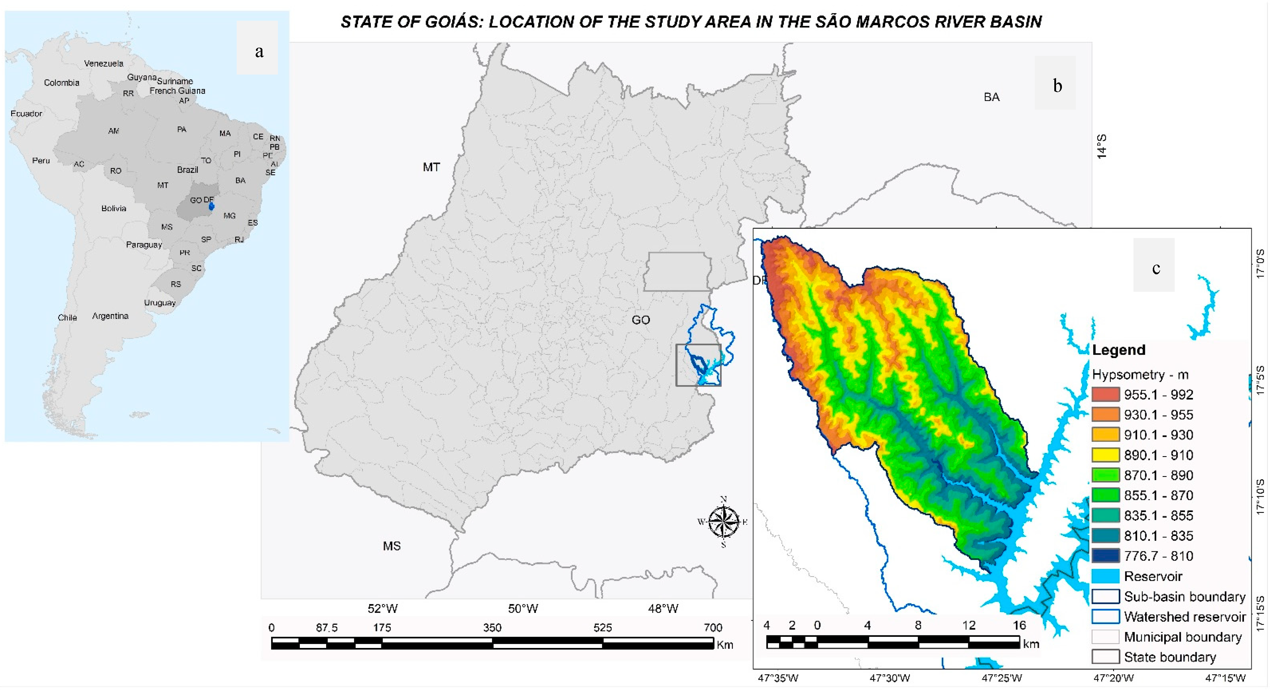
2.1. Location and Characterization of the Study Area

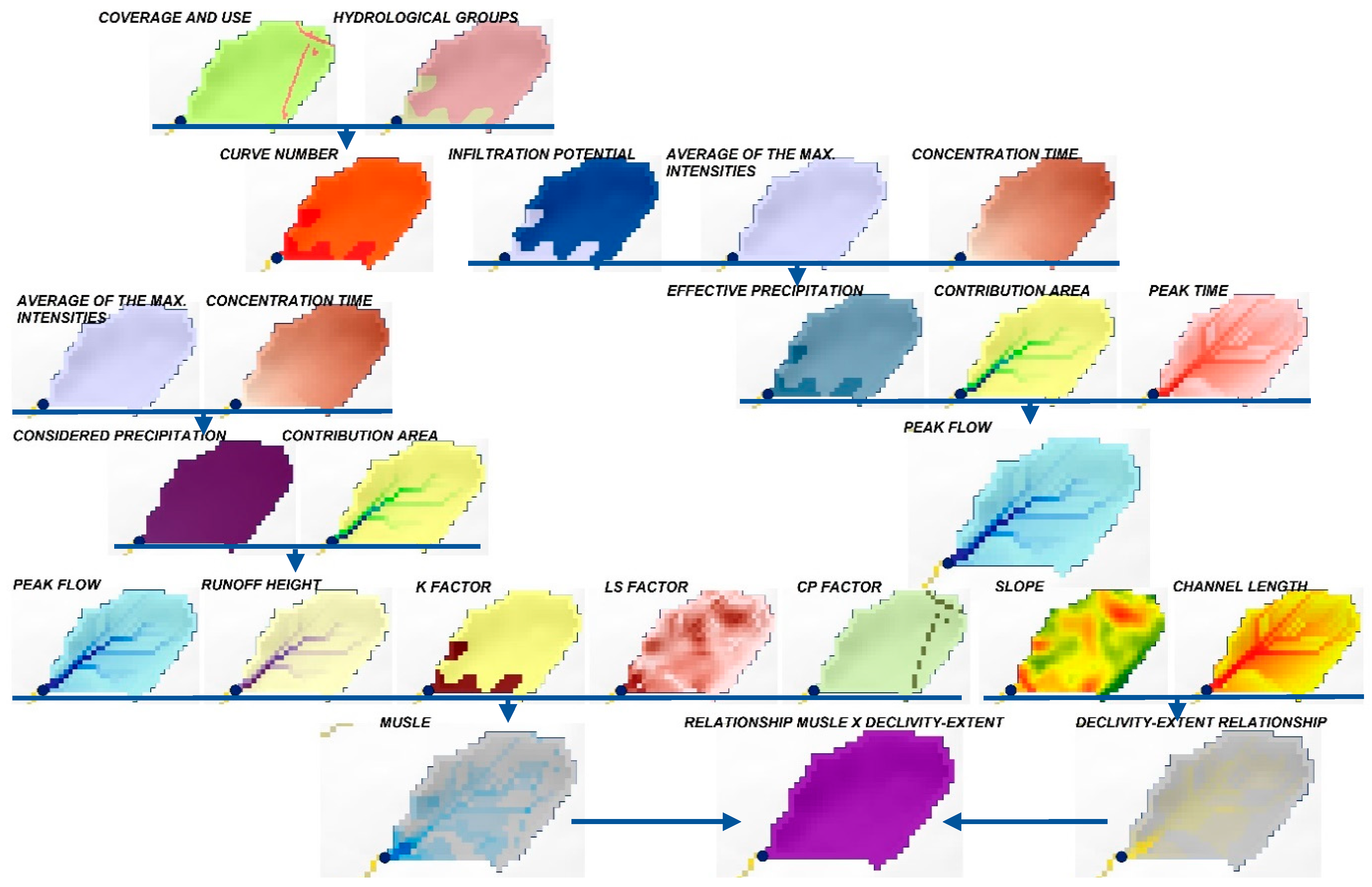
The research area corresponds to the basins of two tributaries of the right bank of the São Firmino River, a tributary of the São Marcos River in the state of Goiás, Midwestern region of Brazil (Figure 1). It comprises an area in which there is extensive and intense agricultural activity, with emphasis on irrigated cultivation [25], as well as small and large reservoirs intended for agricultural activities and hydroelectric power generation [26].

Under the physical aspect, it is characterized by high, residual tops, sometimes flat, supported by detritic–lateritic ferruginous covers composed of clusters of laterites, clay, and sand. The intermediate and steeper segments are associated with the dissection of the Canastra Geological Group—Paracatu Formation, with the predominance of rocks such as sericite and carbonaceous phyllite. Alluvial deposits, composed of sand and gravel, occur in transitioning from these to the lower and flatter parts [27]. In the higher and residual areas, there is a predominance of Plintossols (Petric) with a texture varying from clayey to gravelly, followed, sometimes, by steep segments with the occurrence of Leptsol (Litholic) with sandy to gravelly texture [28,29]. At intermediate altitudes are flatter areas with a predominance of Ferralsol (Red) with a clayey to very clayey texture and, to a lesser extent, Ferralsol (Red-Yellow) with a clayey texture. On the lower levels, with significant slopes in dissected terrains, there is a predominance of Cambisol (Haplic) of clayey to medium texture, sometimes substituted or associated in the steeper segments with Leptsol (Litholic) of sandy to gravelly texture. Along the plains, in low altimetric gradients, there is an association of Fluvisol (Dystrophic) and Gleysol (Haplic).

In general, they are very elongated basins with low circularity index, developed in the form of amphitheaters resulting from the association between the low altimetric gradient in the longitudinal direction and high slopes in the transverse direction. According to Monteiro’s classification [30], the climate of such areas can be recognized as semi-humid tropical, with a dry winter, rainfall of 5.3 to 6.9 mm from June to July, and an average temperature of 24.6 °C during the same period. The summer is hot and rainy, with temperatures around 30.3 °C in October and accumulated precipitation ranging from 243.1 mm to 275.2 mm in January and December [31].

2.2. Methodology

The evaluation of the spatial variability of the sediment production and transfer estimates comprised the bivariate spatial relationship between the soil loss estimates, resulting from the application of the Modified Universal Soil Loss Equation (MUSLE) [32,33,34] and the Declivity-Extent Relationship (DER) proposed by Hack in 1973 [23]. Therefore, the data processing and structuring of the MUSLE variables occurred cumulatively, that is, considering the gradual increase in the contribution area and the spatial variability of each variable involved using geoprocessing procedures. Otherwise, the DER index was applied considering the extension of the channels from the springs to their connection with the reservoir.

2.2.1. Sediment Generation Estimate

The relationship between the MUSLE and the DER index was established from the connection point of each contributing area with its respective channel, allowing each unit to be characterized as the generation, transport, and, consequently, the estimation of sediment input. This approach allowed, besides the simultaneous analysis of two processes, to preserve the application protocols of each model, the MUSLE being applied to the contributing area and slope scale and the DER index at the drainage channel scale. Both models were implemented via geoprocessing in the present work, with the MUSLE applied based on Equation (1).

$$\mathrm{S}=11.8\times {\left(\mathrm{Q}\times \mathrm{pq}\right)}^{0.56}·\mathrm{K}\times \mathrm{LS}\times \mathrm{CP}$$

(1)

where S = estimated soil loss per rainfall event, in tons; Q = runoff volume resulting from the relationship between effective precipitation and contribution area, in m³; pq = peak runoff rate along the rainfall event, in m³/s; K = soil erodibility factor, in t-h MJ⁻¹ mm⁻¹; LS = topographic factor (L is the slope-length factor; and S is the slope-steepness factor, both dimensionless); and CP = land cover and support practice (C is the cover and management factor, and P is the support practice factor, both dimensionless). As it is possible to observe, the soil loss estimation in MUSLE tends to be more accurate in time because it shows more correlation to rainfall conditions, directly related to the volume in runoff and to the flow resulting from the rainfall event.

The spatial variability of surface runoff and peak flow estimates were determined from the effective precipitation. This was determined based on the proposal of the Soil Conservation Service (SCS), now the Natural Resource Conservation Service (NRCS) of the U. S. Department of Agriculture, with its first version published in 1954 [35]. This proposal has undergone several revisions and consists of the ratio between the rainfall resulting from the rainfall event and the infiltration capacity of soils, as presented in Equation (2).

$$\mathrm{Qd}=\left[\frac{{\left(\mathrm{R}-0.2\times \mathrm{S}\right)}^2}{\left(\mathrm{R}+0.8\times \mathrm{S}\right)}\right],\mathrm{as}\mathrm{long}\mathrm{as}\mathrm{P}\ge \mathrm{Ia}=0.2\times \mathrm{S}$$

(2)

where Qd = effective precipitation, or resulting water sheet height, in mm; R = rainfall height resulting from the rainfall event, in mm; S = soil infiltration potential, in mm; and Ia = 0.2 S abstraction or initial loss considered, in mm.

As observed in Equation (2), an initial loss corresponding to 20% of the soil infiltration potential is considered for effective precipitation. This percentage results from interception by plants, retention in the microrelief, and other forms of environmental wetting. Thus, rainfall events that have total precipitation of less than 20% of the soil infiltration potential do not generate runoff.

The rainfall height or accumulated precipitation was determined from the product between the intensity and the duration time of the rainfall event. Following the example of other initiatives [36,37], precipitation intensity was determined using the Intensity–Duration–Frequency (IDF) relationship [38]. For this, the relationship obtained [39] was used for the municipality of Cristalina, as presented in Equation (3).

$$\mathrm{i}=\frac{\mathrm{K}\times {\mathrm{TR}}^{\mathrm{a}}}{{\left(\mathrm{tc}+\mathrm{b}\right)}^{\mathrm{c}}}=\frac{878.213\times {\mathrm{TR}}^{0.2088}}{{\left(\mathrm{t}+12\right)}^{0.7600}}$$

(3)

where i = average of maximum rainfall intensities, in mm/h; TR = return time considered, in years; t = runoff concentration time, in minutes; and K, a, b, and c being adjustment coefficients proper of the climatological station.

To calculate the average maximum rainfall intensities, a return period of 25 years was considered, considering that the present study does not involve safety works and thus allows considering a scenario with a higher probability of occurrence. As for the runoff concentration time, the longest time found among the involved contribution areas was considered. This choice is due to the need to consider a scenario in which the largest contribution area can contribute to the runoff, allowing a condition to be reached for the peak flow. For this, we used the relationship between the flow length on the slopes and the average slope of the basin [40] through Equation (4).

$$\mathrm{Tc}=7.68\times {(\mathrm{L}/{\mathrm{Sw}}^{0.5})}^{0.79}$$

(4)

where Tc = runoff concentration time, in min; L = length of the basin main flow line, in km; and Sw = average basin slope in m/m.

The infiltration potential S was calculated by determining the CN (Curve Number) values according to the Natural Resources Conservation Service (NRCS) [35], as presented in Equation (5).

$$\mathrm{S}=\frac{25400}{\mathrm{CN}}-254$$

(5)

where S = infiltration potential, in mm; CN = Curve Number, dimensionless; and 25,400 and 254 are constants originating from the model.

The CN values were defined according to the evaluation of the soil types, mainly the texture, depth, and classification in Hydrological Groups (

Table 1. Soil classes, texture, and their correspondence in Hydrological Groups and K factor. Source: adapted by authors from [28,29,41,42,43].

Soil Class	Texture	Hydrological Group	K Factor
Cambisol (Dystrophic Haplic)	Clayey to Mean	C	0.0441
Ferralsol (Dystrophic Red)	Clayey to Very Clayey	B	0.0061
Ferralsol (Dystrophic Yellow-Red)	Clayey	B	0.0081
Fluvisol (Dystrophic)	Mean to Sandy	A	0.0290
Plintossol (Concretionary Petric)	Clayey to Gravel	C	0.0438
Leptsol (Dystrophic)	Sandy to Gravel	D	0.0570

), as well as the cover and use conditions. Therefore, the CN values (

Table 2. Land cover and land use types and conditions, Hydrologic Groups, Runoff Number (considering accumulated rainfall greater than 53 mm in the last five days), and CP factor. Source: Prepared by the authors from the multi-spectral Instrument (MSI) sensor of the Sentinel-2 satellite, with passage on 8 June 2020 and adapted from [41,42,44,45].

Coverage and Use Classes	Hydrological Group				CP Factor
	A	B	C	D
	Curve Number
Agriculture—level terracing	60	71	79	82	0.005775
Bare ground—with conservation	62	71	78	81	0.051365
Pasture—medium and low transpiration	47	67	81	88	0.005
Reforestation—medium transpiration	36	60	70	76	0.01635
Forests—dense and high transpiration	26	52	62	69	0.00004
Savannas—medium transpiration	36	60	73	79	0.0007
Permanent grasslands—dense coverage and high transpiration	25	55	70	77	0.01
Permanent grasslands—dense coverage and mean transpiration	36	60	73	79	0.02

) vary from 0 (low flow capacity) to 100 (high flow capacity). Therefore, to calculate the infiltration potential, the soil was in antecedent moisture condition III, which considers accumulated rainfall in the last 5 days greater than 53 mm.

The peak flow rate was determined from the relationship between the effective precipitation, the effective contribution area, and the peak time of the hydrograph [46], as presented in Equation (6).

$$\mathrm{pq}=0.0021\times \mathrm{Qd}\times \mathrm{A}/\mathrm{Tp}$$

(6)

where pq = peak flow along the rainfall event, in m³/s; Qd = effective precipitation or portion of precipitation available for surface runoff, in mm; A = contribution area, in ha; and Tp = peak time of the hydrograph, in hours. The peak time adopted corresponded to 0.6 of the time concentration for each basin, as presented in Equation (7).

$$\mathrm{Tp}=0.6\times \mathrm{Tc}$$

(7)

The LS factor was calculated from the Digital Elevation Model NASADEM HGT v001 [47], with a spatial resolution of 30 m, based on the relationship between flow length and slope [48]. Such a proposal is an adaptation of the classic LS factor. It aims to better represent terrains that have steeper slopes, thus avoiding the overestimation of results due to higher slopes, which is calculated based on the following equation:

$$\mathrm{LS}={(\mathrm{I}/22.13)}^{\mathrm{m}}\times (16.8\times \sin \mathsf{\theta }-0.5)$$

(8)

where I = ramp length, in m; and m = dimensionless exponent calculated using the following equation:

$$\mathrm{m}=\frac{\sin \mathsf{\theta }}{\sin \mathsf{\theta }+0.269\mathrm{x}{(\sin \mathsf{\theta })}^{0.8}+0.05}$$

(9)

where θ = slope, in degrees.

The result of the factor S = 3.0 × (sine θ)^0.8 + 0.56 (for ramp length less than 4 m); S = 10.8 × sine θ + 0.53 (for ramp length greater than 4 m and slope less 9%); S = 16.8 × sine θ − 0.5 (for ramp length greater than 4 m and slope greater than 9%).

It is important to highlight that the calculation of the LS factor was applied to the slope length, as recommended by the methodological orientation. Thus, all the lineaments referring to the fluvial flows were removed so that they would not overestimate the resulting values.

2.2.2. Sediment Transport Capacity Estimates

Estimates of sediment transport capacity were calculated by relating altimetric range and horizontal distance in a given segment as a function of upstream channel length [23] by means of the following equation:

$$\mathrm{DER}=\left(\frac{\Delta \mathrm{h}}{\Delta \mathrm{l}}\right)\times \mathrm{L}$$

(10)

where ∆h = altimetric amplitude between two extreme points of a given segment along the watercourse, in m; ∆l = length or horizontal projection of the length of said segment, in m; and L = total length of the watercourse upstream of the point for which the DER index is being calculated, in km. As explicit in this proposal, the sediment transport capacity is estimated by means of the altimetric gradient of the considered segment, the upstream flow length, and, mainly, the association between the two variables.

The sequential and logical chaining of the methodology adopted in this paper is presented in Figure 2, and it can be divided into four modules. The first corresponds to the rainfall–flow relationship; the second results from applying the MUSLE variables; the third corresponds to the Declivity-Extent Relationship; the fourth to the bivariate relationship between production and sediment transport capacity.

3. Results and Discussion

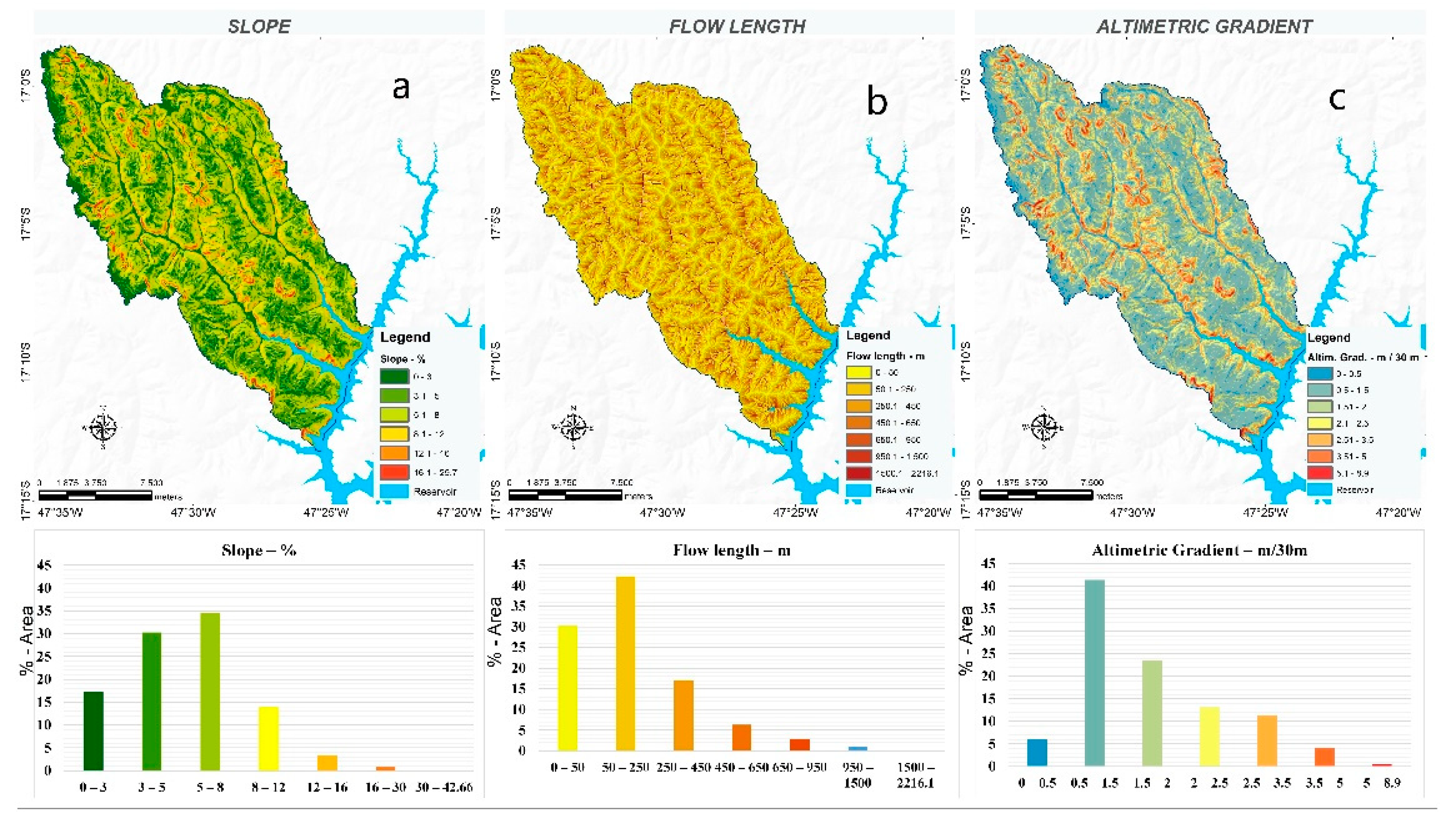
3.1. Morphometric and Morphographic Configuration of the Basins

The study area’s morphometric and morphographic configuration indicates that the development or sculpting of the relief in the four basins occurs predominantly in the longitudinal direction, i.e., following the profile of the main drainage channels. This finding can also be corroborated by the elongated format of the basins, as well as the preservation of the interfluvial tops, resulting in a notable asymmetry between the main channels and their tributaries, which confers a low circularity index.

As observed in part a of Figure 3, the highest slopes tend to occur in the transition between the various altimetric landforms, especially between the highest, dissected one and the intermediate ones. The first occurs in residual hills of the old regional flattening surface, supported by a lithology more resistant to weathering. The second occurs in the form of flatter surfaces with more rounded tops, resulting in lower slopes. Another essential aspect being highlighted refers to the difference between the flow dimensions of the main channels and their tributaries and, mainly, between the two and the length of the slopes, as can be seen in part b of Figure 3. This asymmetry results from the fact that while the area’s slopes have a maximum length of 2.216 km, the present channels have lengths of up to 34.2 km. As a result, the altimetric gradient classes present similar behavior to the slope, with differences concentrated at the edges of the interfluves and mainly at the transition between the altimetric steps, as presented in part c of Figure 3.

The main implication of this slope configuration with the length of slopes and the length of the main channels is the notable difference in the behavior of the altimetric gradient in the transversal and longitudinal directions. In the first direction and starting from the top of the interfluves until reaching the closest channels, the altimetric gradient is more accentuated, which results in high slopes, often occurring in a staggered manner, also resulting from the short length of the slopes. In the longitudinal direction or along the profile of the main channels, the predominance is of a smaller gradient varying from 0 to 0.5 m every 30 m.

On the other hand, the high gradient in the transversal direction resulting from the strong fluvial incision verified at the end of the larger channels, associated with the high declivities resulting from differential erosion that drains directly to the reservoir area implies a greater predisposition to sediment production and transport. For this reason, these environments are more propitious to the configuration of critical areas given the non-existence of dams, the short distance, and the direct contribution to the reservoir. This observation is also valid for environments with a similar configuration close to the backwater areas. In this sense, each sub-basin or contribution area should be evaluated in terms of generation capacity and its respective channel in sediment transport capacity, as presented in the following topics.

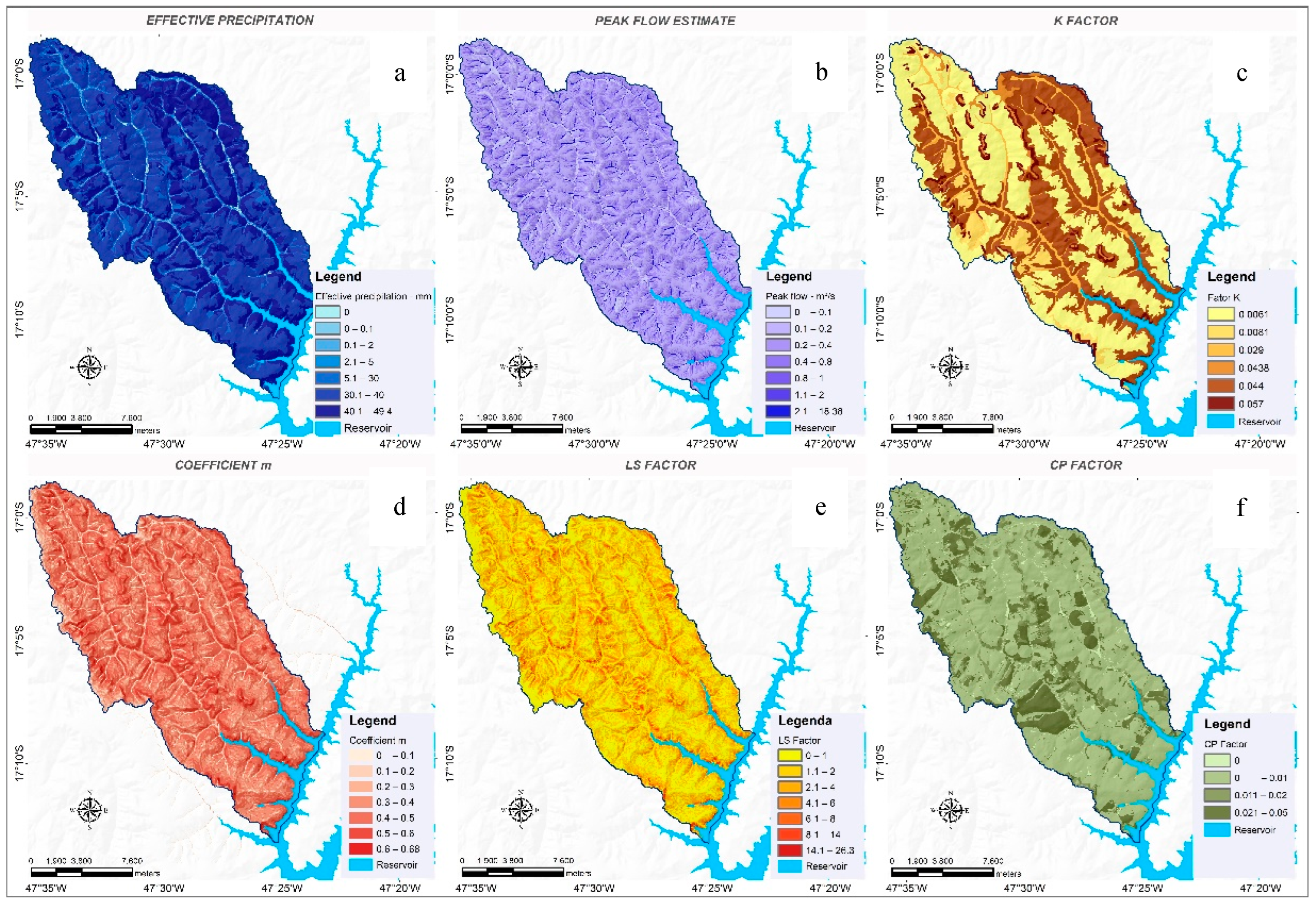
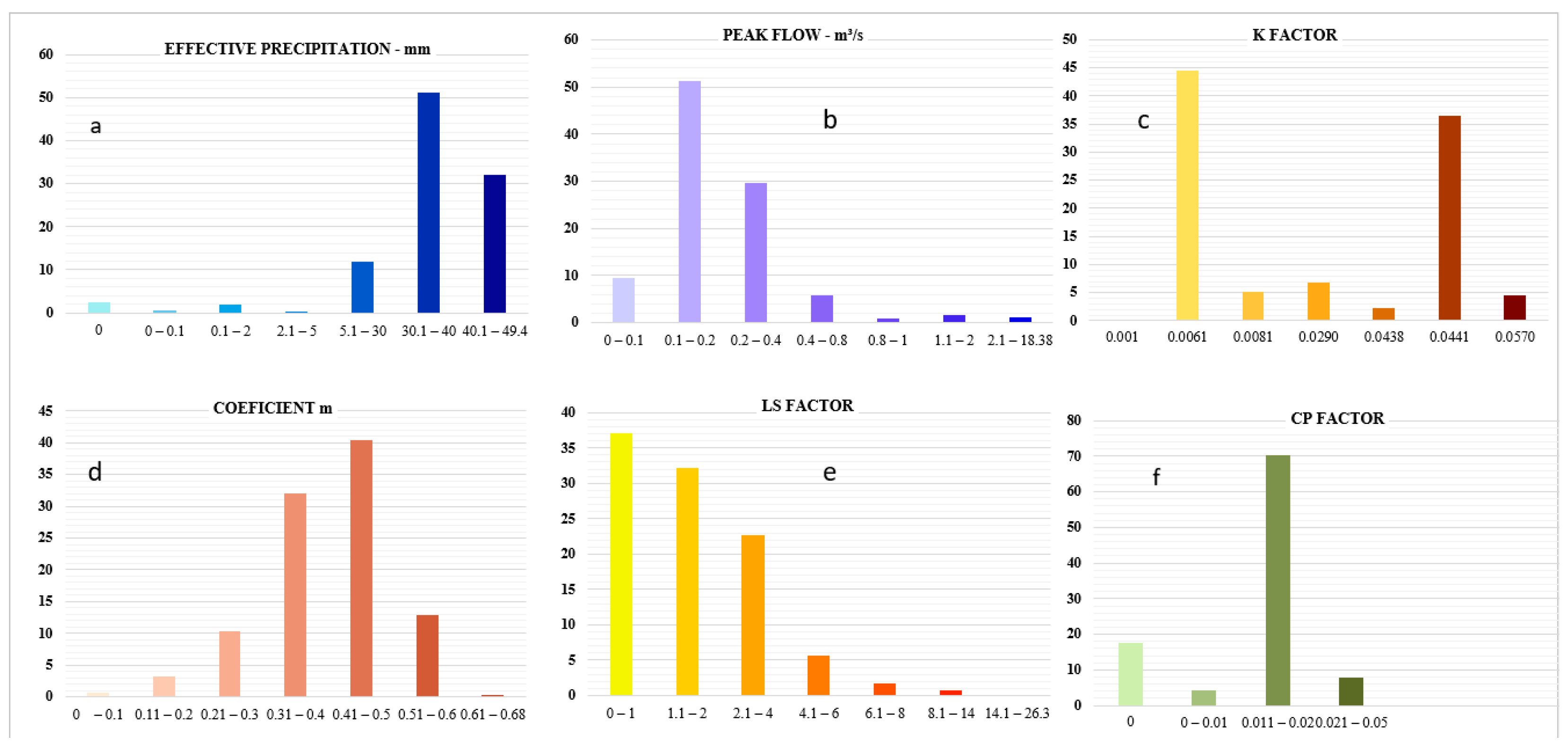
3.2. Rainfall–Runoff Relationship, Soil Erodibility, Topographic Factor, Land Use Cover and Conservation Practices in Sediment Generation Estimates

Considering the relationship between the length of the main flow line and the average slope of each basin in the study area, a maximum concentration time of 46.9 min was reached for the largest specific contribution area, which is about 145.45 ha. With this time and considering the rainfall intensity-duration-frequency equation, a maximum rainfall intensity of 77.56 mm/h was reached, which resulted in an estimated rainfall height of 60.75 mm. Given the characteristics of cover and use and the antecedent humidity considered for the area (5-day precipitation > 53 mm), the effective precipitation ranged from 0 to 49.4 mm, as can be seen in part a of Figure 4.

The portion of precipitation available for the formation of surface runoff was notoriously low in the lower areas, flat areas with sandy soils and larger vegetation cover. The most expressive values, ranging from 40 to 49.4 mm, were predominant in the steepest areas, with less developed soils where savannah and grassland formations occur.

As for the runoff volume estimates, the classes’ spatial behavior tends to correlate with effective precipitation behavior. However, the configuration of the lateral flow lines conditions a gradual increase in the downstream flow due to the increase in the effect provided by the specific contribution area. Under these conditions, the estimates of peak flows ranged from 0 m³/s—at the water dividers—to 18.38 m³/s at the point of maximum flow convergence of the largest specific contribution area, as shown in part b of Figure 4. As for the erodibility classes of the soils, one can see that they have a considerable correlation with the classes of coefficient m and the LS factor. The less developed soils with greater erodibility tend to occur associated with the classes of the greater slope. This is one of the reasons why the more erodible soils are related to the classes with a higher LS factor, resulting in a cumulative effect of soil loss. The exception is the Fluvisol, whose occurrence is associated with the low altimetric gradient prevailing along the floodplains. Given this physical–hydrological configuration, it should be emphasized that the using the area for agricultural activities with adequate management factors contributes to low CP factor values—0.01 to 0.02—in most of the basin areas. The classes of each component variable of the MUSLE and their respective percentages of area occurrence are shown in Figure 5.

3.3. Bivariate Relationship between Estimates of Sediment Generation and Transport Capacity

Considering the established hydrological conditions and their relation to soil erodibility, as well as the cover and use conditions of the area, we arrived at generation estimates ranging from 0 to, exceptionally, 115.43 tons of sediment. The lowest estimates are predominantly distributed in the central and higher portion of the interfluves. These environments are marked by the predominance of low slopes, still incipient flows, and little specific contribution area. However, it is already possible to observe estimates of more developed flows with steeper slopes and, especially, a larger area of contribution in the intermediate portions of the slopes. This can influence the volume available for surface runoff and, consequently, increase erosive power. In this sense, the segments with more accentuated values correspond to those that mark the transition from the slopes to their respective drainage channels. In the research area, the most critical point corresponds to that under the hydrological effects of a contribution area with approximately 145.45 ha, which resulted in an estimate of 115.43 tons, as highlighted in the blue rectangle in Figure 6. Similarly, the high sediment transport potentials—44.16—also occur preferentially in lower-order basins, as observed in the yellow rectangle of the same figure. The reason for their occurrence in a more localized way resides in the fact that the equation used for their calculation does not consider the hydrological conditions and, mainly, the gradual effect of the upstream area, resulting in classes with a more linear format.

From the association of these two components—estimation and sediment transport capacity—it is possible to perceive contribution basins in four distinct situations, as illustrated in part c of Figure 6.

One result from the low estimate of yield and low sediment transfer potential, resulting from flat surfaces with little surface runoff, is a little area of contribution that predominates in most of the area; another is related to the low estimate of yield and high sediment transfer capacity resulting from steep surfaces, but without a large area of contribution; another formed by the high estimate of contribution, but the low capacity of sediment transfer, resulting from the convergence of large areas of contribution, of more erodible soils, with inadequate management, predominates from the intermediate third to the lower third of the slopes; and another, more worrying one, resulting from the convergence of situations of high production estimate, as well as of high capacity of sediment transfer, whose occurrence tends to concentrate in the segments of convergence of the slopes with the drainage channels.

Of all the situations reported, the one resulting from high estimated production and sediment transport capacity, whose drainage occurs directly into the reservoir, deserves to be highlighted. This situation represents a greater probability of direct impact in a short period of time, both at the edges and in the backwater areas. For this reason, these areas require greater attention through continuous monitoring, as well as priority concerning improvements in soil management practices.

4. Concluding Remarks

The improvement and application of predictive models, such as the SCS method, is an increasingly efficient strategy to support the evaluation of phenomena involving runoff, generation, transport, and sediment input. This is extremely necessary when one aims to evaluate hydrographic systems with thousands of square kilometers, such as the contribution basins of large reservoirs, without losing sight of the level of detail required for analysis at the slope scale and its cumulative effects on the other scales of analysis. It constitutes a primordial step for evaluating systems that present a complex chain of processes involving the shape of the slopes, the profiles of drainage channels, and the area of the hydrographic systems’ contribution basins [49].

Even when it comes to predictive situations when supported by basic maps of incredible precision that allow considering the pedological, geomorphological, hydrological [50], climatological [51], land cover, land use, and management conditions in excellent levels of detail [52] offer results for the elaboration of increasingly accurate diagnoses and prognoses, especially considering the spatial-temporal variability of land cover and land use changes [53] and meteorological conditions [54]. The use of these materials at an excellent level of detail via geoprocessing resources allows weighting of the spatiotemporal variability of constraints and their application for large areas without losing the sophistication and efficiency of the SCS method [55]. Consequently, they reduce the uncertainties of the predictions [56] and allow the identification of critical areas and, therefore, priority areas for monitoring and adequate soil management, resulting in greater efficiency in the use of water resources. The calibration process is always recommended [57], and the results can be compared, for example, with suspended sediments or turbidity at reservoir edges [58], allowing us to reach increasingly more comprehensive results.

In this case, it was possible to identify with a considerable level of detail the relation between the main conditioning factors of sediment generation, the transport capacity along each drainage channel, and the resulting potential contribution of each basin. Thus, it was observed that a low estimate of sediment generation and low sediment transport capacity predominated in most of the area; a low estimate of generation and high sediment transport capacity occurred mainly in the steeper segments and close to the channels; a high estimate of generation and low transport capacity related to the areas of higher altitudes and intermediate thirds of the slopes; and high estimate of generation, as well as high transport capacity, whose occurrence in the immediate vicinity or even in the direct contribution basins draw more attention to degradation by erosive processes and sedimentological impacts.

It is understood that the representation of the spatial variability of the estimates of production and transport of sediments indicates areas with distinct levels of potential sediment contribution and, consequently, priority for field evaluations and better dimensioning of hydrosedimentological imbalances. This can subsidize the elaboration of monitoring projects and the definition of best practices for soil use and management to contribute to reducing sediment inputs and, consequently, maintain the efficiency and useful life of large reservoirs.

The proposed methodological contribution presented here is focused on sediment generation and transport along the tributaries of HPP (Hydroelectric Power Plant) contributing basins. As mitigating measures to reduce soil loss, it is proposed to improve soil management practices in the basins with the greatest potential for sediment generation and transport. Complementarily, it is known that from an integrated point of view, the debris generated needs to flow gradually along the fluvial system, obeying the natural tendency of the relationship between soil erosion, relief sculpturing, and material transport via drainage channels. The sediments generated and transported tend to be deposited initially on the less steep banks and in the backwater areas (low gradient segments that connect the channels with the reservoir). Another deposition point refers to the dam (structure installed to the dam and raises the water level). Overcoming, even if only partially, the effects of these two deposition environments requires a direct connection between the upstream portions and the dam section, in this case, at the dam’s base, allowing the sediment flow to continue downstream. In practice, this would be like installing submerged pipelines connecting the backwater areas and a passage under the dam structure. In this sense, testing this hypothesis and evaluating its efficiency is an important field to be investigated.

References

1. Liu, C.; Walling, D.E.; He, Y. Review: The International Sediment Initiative case studies of sediment problems in river basins and their management. Int. J. Sediment Res. 2018, 33, 216–219. [Google Scholar] [CrossRef]
2. Ayele, G.T.; Kuriqi, A.; Jemberrie, M.A.; Saia, S.M.; Seka, A.M.; Teshale, E.Z.; Daba, M.H.; Ahmad Bhat, S.; Demissie, S.S.; Jeong, J.; et al. Sediment Yield and Reservoir Sedimentation in Highly Dynamic Watersheds: The Case of Koga Reservoir, Ethiopia. Water 2021, 13, 3374. [Google Scholar] [CrossRef]
3. Phuong, T.T.; Shrestha, R.P.; Chuong, H.V. Simulation of Soil Erosion Risk in the Upstream Area of Bo River Watershed. In Re-Defining Diversity and Dynamism of Natural Resource Management in Asia; Thang, T.N., Dung, N.T., Hulse, D., Sharma, S., Shivakoti, G.P., Eds.; Elsevier: Amsterdam, The Netherlands, 2017; Volume 3, pp. 87–99. [Google Scholar] [CrossRef]
4. Wang, H.W.; Kondolf, M.; Tullos, D.; Kuo, W.C. Sediment Management in Taiwan’s Reservoirs and Barriers to Implementation. Water 2018, 10, 1034. [Google Scholar] [CrossRef] [Green Version]
5. Fox, G.A.; Sheshukov, A.; Cruse, R.; Kolar, R.L.; Guertault, L.; Gesh, K.R.; Dutnell, R.C. Reservoir Sedimentation and Upstream Sediment Sources: Perspectives and Future Research Needs on Streambank and Gully Erosion. Environ. Manag. 2016, 57, 945–955. [Google Scholar] [CrossRef] [Green Version]
6. Iradukunda, P.; Bwambale, E. Reservoir sedimentation and its effect on storage capacity–A case study of Murera reservoir, Kenya. Cogent Eng. 2021, 8, 1. [Google Scholar] [CrossRef]
7. Obialor, C.A.; Okeke, O.C.; Onunkwo, A.A.; Fagorite, V.I.; Ehujuo, N.N. Reservoir Sedimentation: Causes, Effects and Mitigation. Int. J. Adv. Acad. Res.–Sci. Technol. Eng. 2019, 5, 92–109. [Google Scholar]
8. Benavidez, B.; Jackson, B.; Maxwell, D.; Norton, K. A review of the (Revised) Universal Soil Loss Equation ((R)USLE): With a view to increasing its global applicability and improving soil loss estimates. Hydrol. Earth Syst. Sci. 2018, 22, 6059–6086. [Google Scholar] [CrossRef] [Green Version]
9. Ezzaouini, M.A.; Mahé, G.; Kacimi, I.; Zerouali, A. Comparison of the MUSLE Model and Two Years of Solid Transport Measurement, in the Bouregreg Basin, and Impact on the Sedimentation in the Sidi Mohamed Ben Abdellah Reservoir, Morocco. Water 2020, 12, 1882. [Google Scholar] [CrossRef]
10. Arekhi, S.; Shabani, A.; Rostamizad, G. Application of the modified universal soil loss equation (MUSLE) in prediction of sediment yield (Case study: Kengir Watershed, Iran). Arab. J. Geosci. 2012, 5, 1259–1267. [Google Scholar] [CrossRef]
11. Kumar, P.S.; Praveen, T.V.; Prasad, M.A. Simulation of Sediment Yield over Un-gauged Stations Using MUSLE and Fuzzy Model. Aquat. Procedia 2015, 4, 1291–1298. [Google Scholar] [CrossRef]
12. Colman, C.B.; Garcia, K.M.P.; Pereira, R.B.; Shinma, E.A.; Lima, F.E.; Gomes, A.O.; Oliveira, P.T.S. Different approaches to estimate the sediment yield in a tropical watershed. Braz. J. Water Resour. 2018, 23, e47. [Google Scholar] [CrossRef] [Green Version]
13. Morris, G.L. Classification of Management Alternatives to Combat Reservoir Sedimentation. Water 2020, 12, 861. [Google Scholar] [CrossRef] [Green Version]
14. Thomas, K.; Chen, W.; Lin, B.-S.; Seeboonruang, U. Evaluation of the SEdiment Delivery Distributed (SEDD) Model in the Shihmen Reservoir Watershed. J. Sustain. 2020, 12, 6221. [Google Scholar] [CrossRef]
15. Miranda, L.E. Reservoir Fish Habitat Management; Lightning Press: Totowa, NJ, USA, 2017. [Google Scholar]
16. De Rosa, P.; Fredduzzi, A.; Cencetti, C. Stream Power Determination in GIS: An Index to Evaluate the Most ‘Sensitive’ Points of a River. Water 2019, 11, 1145. [Google Scholar] [CrossRef] [Green Version]
17. Yuan, X.P.; Braun, J.; Guerit, L.; Rouby, D.; Cordonnier, G. A New Efficient Method to Solve the Stream Power Law Model Taking Into Account Sediment Deposition. J. Geophys. Res. Earth Surf. 2019, 124, 1346–1365. [Google Scholar] [CrossRef] [Green Version]
18. Song, S.; Schmalz, B.; Fohrer, N. Simulation and comparison of stream power in-channel and on the floodplain in a German lowland area. J. Hydrol. Hydromech. 2014, 62, 133–144. [Google Scholar] [CrossRef] [Green Version]
19. Whipple, K.X.; Tucker, G.E. Dynamics of the stream-power river incision model: Implications for height limits of mountain ranges, landscape response timescales, and research needs. J. Geophys. Res. Solid Earth 1999, 104, 17661–17674. [Google Scholar] [CrossRef]
20. Albo-Salih, H.; Mays, L.W.; Che, D. Application of an Optimization/Simulation Model for the Real-Time Flood Operation of River-Reservoir Systems with One-and Two-Dimensional Unsteady Flow Modeling. Water 2022, 14, 87. [Google Scholar] [CrossRef]
21. Vente, J.; Poesen, J.; Arabkhedri, M.; Verstraeten, G. The sediment delivery problem revisited. Prog. Phys. Geogr. Earth Environ. 2007, 31, 155–178. [Google Scholar] [CrossRef] [Green Version]
22. Mishra, K.; Sinha, R.; Jain, V.; Nepal, S.; Uddin, K. Towards the assessment of sediment connectivity in a large Himalayan River basin. Sci. Total Environ. 2019, 661, 251–265. [Google Scholar] [CrossRef]
23. Hack, J.T. Stream-profile analysis and stream-gradient index. J. Res. U.S. Geol. Surv. 1973, 1, 421–429. [Google Scholar]
24. Mitasova, H.; Barton, M.; Ullah, I.; Hofierka, J.; Harmon, R.S. GIS-Based Soil Erosion Modeling. In Treatise on Geomorphology; Shroder, J.F., Ed.; Academic Press: San Diego, CA, USA, 2013; Volume 3, pp. 228–258. [Google Scholar] [CrossRef]
25. Pereira Júnior, L.C.; Ferreira, N.C.; Miziara, F. A Expansão da Irrigação Por Pivôs Centrais no Estado de Goiás (1984–2015). Bol. Goiano Geogr. 2017, 37, 323–341. [Google Scholar] [CrossRef] [Green Version]
26. Nunes, E.D.; Romão, P.A.; Sales, M.M.; Luz, M.P. Geoprocessing Applied in the Estimate of Infiltration and Surface Runoff in HPP’s Contribution Watershed. J. Geogr. Inf. Syst. 2021, 13, 643–659. [Google Scholar] [CrossRef]
27. Faria, A. Geologia do Domo de Cristalina, Goiás. Rev. Bras. Geociências 1985, 15, 231–240. [Google Scholar] [CrossRef]
28. Resende, M.J.G. Classes de Solos dos Municípios Goianos–2016; EMATER: Goiânia, Brazil, 2016. [Google Scholar]
29. Rosa, L.E.; Santos, N.B.F.; Bayer, M.; Castro, S.S.; Nunes, E.D.; Cherem, L.F.S. Atributos Para Mapeamento Digital de Solos: O Estudo de Caso na Bacia do Ribeirão Arrojado, Município de Cristalina–Goiás. In Elementos da Natureza e Propriedades dos Solos; Oliveira, A.C., Ed.; Atena Editora: Ponta Grossa, Brazil, 2018; pp. 68–82. [Google Scholar] [CrossRef]
30. Monteiro, C.A.F. Notas para o estudo do clima do Centro-Oeste Brasileiro. Rev. Bras. Geogr. 1951, 13, 3–46. [Google Scholar]
31. Novais, G.T. Climate Classification Applied to the State of Goiás and the Federal District, Brazil. Bol. Goiano Geogr. 2020, 40, 1–29. [Google Scholar]
32. Williams, J.R. Sediment-Yield Prediction with Universal Equation Using Runoff Energy Factor. In Present and Prospective Technology for Predicting Sediment Yield and Sources; USDA–Agriculture Research Service: Washington, DC, USA, 1975; pp. 244–252. [Google Scholar]
33. Williams, J.R. Testing the modified Universal Soil Loss Equation. In Proceedings of the Workshop on Estimating Erosion and Sediment Yield on Rangelands; USDA–Agriculture Research Service: Tucson, AZ, USA, 1981; pp. 157–165. [Google Scholar]
34. Smith, S.J.; Williams, J.R.; Menzel, R.G.; Coleman, G.A. Prediction of sediment yield from Southern Plains Grasslands with the Modified Universal Soil Loss Equation. Rangel. Ecol. Manag. J. 1984, 37, 295–297. [Google Scholar] [CrossRef]
35. NRCS—Natural Resources Conservation Service. National Engineering Handbook, Part 630 Hydrology, Chapter 10 Estimation of Direct Runoff from Storm Rainfall; USDA: Washington, DC, USA, 2004; pp. 1–79. [Google Scholar]
36. Sun, Y.; Wendi, D.; Kim, D.E.; Liong, S.-Y. Deriving intensity–duration–frequency (IDF) curves using downscaled in situ rainfall assimilated with remote sensing data. Geosci. Lett. 2019, 6, 17. [Google Scholar] [CrossRef] [Green Version]
37. Balmaceda, E.G.; López-Ramos, A.; Martínez-Acosta, L.; Medrano-Barboza, J.P.; López, J.F.R.; Seingier, G.; Daesslé, L.W.; López-Lambraño, A.A. Rainfall Intensity-Duration-Frequency Relationship. Case Study: Depth-Duration Ratio in a Semi-Arid Zone in Mexico. Hydrology 2020, 7, 78. [Google Scholar] [CrossRef]
38. Villela, S.M.; Mattos, A. Hidrologia Aplicada; McGrawHill do Brasil: São Paulo, Brazil, 1975; p. 245. [Google Scholar]
39. Oliveira, L.F.C.; Cortês, F.C.; Wehr, T.R.; Borges, L.B.; Sarmento, P.H.L.; Griebeler, N.P. Intensidade-Duração-Frequência de Chuvas Intensas Para Localidades no Estado de Goiás e Distrito Federal. Pesqui. Agropecuária Trop. 2005, 35, 13–18. [Google Scholar]
40. Watt, W.E.; Chow, K.C.A. A General Expression for Basin Lag Time. Can. J. Civ. Eng. 1985, 12, 294–300. [Google Scholar] [CrossRef]
41. Tucci, C.E.M. Águas urbanas. Estud. Avançados 2008, 22, 97–112. [Google Scholar] [CrossRef]
42. Tucci, C.E.M.; Marques, D.M.L.M. Avaliação e Controle da Drenagem Urbana; UFRGS: Porto Alegre, Brazil, 2000; 558p. [Google Scholar]
43. Mannigel, A.R.; Carvalho, M.P.; Moreti, D.; Medeiros. Fator erodibilidade e tolerância de perda dos solos do Estado de São Paulo. Acta Sci. Agron. 2002, 24, 1335–1340. [Google Scholar] [CrossRef]
44. Stein, D.P.; Donzelli, P.L.; Gimenez, F.A.; Ponçano, E.L.; Lombardi Neto, F. Potencial de Erosão Laminar, Natural e Antrópica na Bacia do Peixe-Paranapanema. In Simpósio Nacional de Controle de Erosão; ABGE: Marília, Brazil, 1987; pp. 105–135. [Google Scholar]
45. Oliveira, J.S. Avaliação de Modelos de Elevação na Estimativa de Perda de Solos em Ambiente SIG. Master’s Thesis, Escola Superior de Agricultura Luiz de Queiroz—Universidade de São Paulo, Piracicaba, Brazil, 2012. [Google Scholar]
46. Schwab, G.O.; Fangmeier, D.D.; Elliot, W.J.; Frevert, R.K. Soil and Water Conservation Engineering, 4th ed.; John Wiley & Sons: Chichester, UK, 1993; p. 528. [Google Scholar]
47. NASA JPL. NASADEM Merged DEM Global 1 arc Second V001 [Data Set] 2020. Distributed by NASA EOSDIS Land Processes DAAC. Available online: https://lpdaac.usgs.gov/products/nasadem_hgtv001/ (accessed on 2 April 2021). [CrossRef]
48. McCool, D.K.; Brown, L.C.; Foster, G.R.; Mutchler, C.K.; Meyer, L.D. Revised slope steepness factor for the Universal Soil Loss Equation. Trans. Am. Soc. Agric. Biol. Eng. 1987, 30, 1387–1396. [Google Scholar] [CrossRef]
49. Kand, M.; Yoo, C. Application of the SCS–CN Method to the Hancheon Basin on the Volcanic Jeju Island, Korea. Water 2020, 12, 3350. [Google Scholar] [CrossRef]
50. Caletka, M.; Michalková, M.S.; Karásek, P.; Fucík, P. Improvement of SCS-CN Initial Abstraction Coefficient in the Czech Republic: A Study of Five Catchments. Water 2020, 12, 1964. [Google Scholar] [CrossRef]
51. Krajewski, A.; Sikorska-Senoner, A.; Hejduk, A.; Hejduk, L. Variability of the Initial Abstraction Ratio in an Urban and an Agroforested Catchment. Water 2020, 12, 415. [Google Scholar] [CrossRef] [Green Version]
52. Shi, W.; Wang, N. An Improved SCS-CN Method Incorporating Slope, Soil Moisture, and Storm Duration Factors for Runoff Prediction. Water 2020, 12, 1335. [Google Scholar] [CrossRef]
53. Psomiadis, E.; Soulis, K.X.; Efthimiou, N. Using SCS-CN and Earth Observation for the Comparative Assessment of the Hydrological Effect of Gradual and Abrupt Spatiotemporal Land Cover Changes. Water 2020, 12, 1386. [Google Scholar] [CrossRef]
54. Mlynski, D.; Walega, A.; Ksiazek, L.; Florek, J.; Petroslli, A. Possibility of Using Selected Rainfall-Runoff Models for Determining the Design Hydrograph in Mountainous Catchments: A Case Study in Poland. Water 2020, 12, 1450. [Google Scholar] [CrossRef]
55. Ajmal, M.; Waseem, M.; Kim, D.; Kim, T.-W. A Pragmatic Slope-Adjusted Curve Number Model to Reduce Uncertainty in Predicting Flood Runoff from Steep Watersheds. Water 2020, 12, 1469. [Google Scholar] [CrossRef]
56. Soulis, K.X. Soil Conservation Service Curve Number (SCS-CN) Method: Current Applications, Remaining Challenges, and Future Perspectives. Water 2021, 13, 192. [Google Scholar] [CrossRef]
57. Ling, L.; Yusop, Z.; Yap, W.-S.; Tan, W.L.; Chow, M.F.; Ling, J.L. A Calibrated, Watershed-Specific SCS-CN Method: Application to Wangjiaqiao Watershed in the Three Gorges Area, China. Water 2020, 12, 60. [Google Scholar] [CrossRef] [Green Version]
58. Cui, M.; Sun, Y.; Huang, C.; Li, M. Water Turbidity Retrieval Based on UAV Hyperspectral Remote Sensing. Water 2022, 14, 128. [Google Scholar] [CrossRef]
Figure 1. (a) Location of Brazil in South America, (b) State of Goiás—Midwestern Region of Brazil, and (c) right margin of the São Firmino River.
Water 14 04091 g001
Figure 2. Sequential and logical flowchart of the methodological steps adopted in the development of this article.
Water 14 04091 g002
Figure 3. Map of slope (a); of flow length (b); and altimetric gradient (c), considering a standard horizontal distance of 30 m.
Water 14 04091 g003
Figure 4. Spatial variability of MUSLE factors: effective precipitation (a); peak flow (b); soil erodibility (c); m coefficient (d); LS factor (e); and CP factor (f).
Water 14 04091 g004
Figure 5. Classes of effective precipitation (a); peak flow (b); soil erodibility (c); m coefficient (d); LS factor (e); CP factor (f) and respective percentages of coverage areas.
Water 14 04091 g005
Figure 6. Distribution of the variable soil loss estimate (part a); distribution of the variable sediment transfer capacity (part b); and resulting from the combination of soil loss estimate × sediment transport capacity (part c).
Water 14 04091 g006