
Application of the HEC-RAS Program in the Simulation of the Streamflow Hydrograph for Air Lakitan Watershed

1
Department of Civil and Environmental Engineering, Universitas Bina Darma, Palembang 30264, Indonesia
2
Department of Civil and Environmental Engineering, Nazarbayev University, Astana 010000, Kazakhstan
3
Department of Civil Engineering, Indo Global Mandiri University, Palembang 30129, Indonesia
*
Author to whom correspondence should be addressed.
Water 2022, 14(24), 4094; https://doi.org/10.3390/w14244094
Submission received: 21 October 2022
/
Revised: 8 December 2022
/
Accepted: 9 December 2022
/
Published: 15 December 2022
(This article belongs to the Section Hydrology)
Abstract
:Floods are an issue that results in losses, and thus attempts to solve the problem of flooding are attempts to minimize losses. To mitigate the losses incurred as much as possible, there are several approaches to deal with the loss through incident management and its impacts. The objective of this study is to investigate the variations in water level within Air Lakitan Watershed to monitor the fluctuations of water level for preventing flooding issues in the future. This research was carried out by analyzing the hydrodynamics of flow in irrigation canals in Irrigation Area II with an area of 928 hectares using the HEC-RAS program with rainfall data and flow hydraulics data. The study was carried out in Air Lakitan Watershed in Sumber Harta District, Musi Rawas Regency, Sumatra, Indonesia. Each portion of the studied irrigation canal’s water level and velocity, as measured by a current meter, are shown on graphs, as are the study’s overall conclusions for each observation station along the channel. Simulated data was acquired using a river crossing that is not filled and a discharge of 0.024 m3/s. From this research, it can be concluded that the Log-Pearson Type III distribution is the frequency distribution that matches the hydrological analysis in the research area. This method can be applied in analyses of river levels in other areas with heavy rainfall. Therefore, the water level upstream and downstream is the same at 0.41 m with a discharge of 1 m3/s; the river cross-section downstream with an existing discharge of 0.024 m3/s produces water height as high as 0.08 m and with a flow rate of 0.783 m/s, the water level at the downstream cross-section is filled up to 0.75 m high, and the water level downstream of the irrigation channel is up to 0.40 m.
1. Introduction
The Kelingi watershed, the Semangus watershed, the Air Lakitan Watershed, and the Musi watershed are just a few of the water sources that feed the region’s 254 rivers, both big and tiny. The water in these rivers can be used for any purpose, but it can also cause problems, like floods, if it is not managed properly. Musi Rawas Regency’s Public Works, Irrigation Service, Spatial Planning, and Cipta Karya will be better able to use and regulate the river system with the collected data and river profile. Natural factors like heavy precipitation, sloping land, and the effect of tides are common factors resulting in flooding within a watershed or region. Human actions, such as settlement in low-lying areas near rivers or having factories dispose of their waste in waterways, frequently contribute to flood issues [1,2,3].
Inadequate river/drainage system management and/or poor maintenance are also factors contributing to the flooding problem. As a result of societal issues, more and better home environmental infrastructure is needed. A left/right inspection road design, integrated structural and non-structural riverbank reclamation and installation in Musi Rawas Regency, and immediate program outputs are required to address the issues outlined above [1,4]. In this way, it is to everyone’s advantage to work on the natural factors that lead to flooding in a given location, such as by making use of natural flow-retaining zones (retarding ponds) and spatial/land planning.
Musi Rawas Regency as a whole has an area of 1,236,582.66 Ha. The area is part of Muara Lakitan District with an area of 15.88 percent of the total area of the district. In general, the Musi Rawas Regency area has a diverse topography, ranging from lowlands to highlands. The altitude of the area ranges from 25–1000 m above sea level and has a tropical and wet climate with an average monthly rainfall of 200 mm based on the data for 15 years with an average of 11 rainy days per month. The highest average rainfall and the rainiest days occur in December, which averages 382 mm and 19 rainy days [1,4].
The Musi Rawas district is fed by five main rivers that are generally navigable, namely, the Musi River, Rawas River, Lakitan River, Kelingi River, and Semangus River. In addition, other rivers are tributaries of the main rivers, such as the Keruh River, the Lintang River, and the Kungku River, which is a tributary of the Musi River [1,4]. In addition to having large rivers, in the Musi Rawas district there are also several lakes, including Raya Lake in Rupit sub-district and Aur Lake in Sumber Harta sub-district, which function as water reservoirs, and these lakes also have tourism potential for Musi Rawas district.
Musi Rawas Regency’s river channels are in relatively good shape, meaning that they can accommodate flows of varying intensities and can even be used as river transportation routes. However, the river’s flow is severely impeded by the many places that are used as fishponds. As river levels rise, floods become more common as flow capacity is reduced. The overflow of the river will also cause flooding in several neighborhoods. That is why it is so important to check with the local authorities about whether or not there are any hard and fast rules on how the river channel is supposed to work [5,6].
Because the river channel is full of big tree branches that hinder the flow of the river and function as a factor limiting its flow capacity, there is damage to river channels and cliffs in some regions, particularly near river bends. The river in Musi Rawas Regency overflowed its banks several years ago (around 2008), causing widespread flooding in the region. An average flood can reach a height of about a meter and linger for as long as two days (results of interviews with residents). Smaller rivers gather and transmit runoff from roads and other urban areas, complementing the larger rivers. There have been reports that the storage capacity of the rivers in the Musi Rawas Regency is insufficient to evacuate the rainwater during times of heavy rainfall [5,7].
Homes were rendered uninhabitable due to flooding, public health was compromised due to the spread of numerous diseases, and transportation and the local economy were rendered inoperable as a result of the flood catastrophe in the Musi Rawas Regency. Incapable of regular mobility, many animals were lost or killed, and much property was destroyed. Because not all of the natural drainage channels or small rivers in the area have been revitalized according to conventional design, the flooding problem is exacerbated whenever there is heavy rainfall [5] lasting between one and three hours and the water from the natural drainage or small rivers overflows and fills the entire area. At the same time, the low basin carries sediment to the unplanned drainage channel, which eventually empties into the river as the “mainstream” in Musi Rawas Regency [5,8].
Since floods cannot be eliminated, the goal of flood preventive activities (flood loss management) is to reduce losses brought on by floods. The objective of this study is to investigate the variation of water levels within Air Lakitan Watershed. This research was carried out by analyzing the hydrodynamics of flow in irrigation canals in Irrigation Area II with an area of 928 hectares using the HEC-RAS program with rainfall data and flow hydraulics data.
2. Methods
2.1. Data and Investigation
This survey was carried out after studying maps that were the result of the secondary data collection stages. This survey was designed to get a clearer picture of the details of damage to existing weirs and to estimate the potential for improved dam function in the future. Data was obtained in this survey including:
- Location (administrative, coordinates, river name, and others).
- Determination of the measurement location boundary and topographic reference point.
- Water sources and irrigation water availability.
- Condition of irrigation networks (maps and schemes).
- Irrigation management status.
- Water supply, distribution, and water supply plans, cropping plans, drying plans, etc.
- Estimated area of the service area to be irrigated.
- Estimated benefits derived from plans for building a water divider building (tapping building).
- Institutional irrigation Operation and Maintenance (OM).
2.2. Research Location
3. Hydrograph Stream Flow Analysis
The Deras II Irrigation Area, which among other things aims to drain the water discharge, includes the Moyan weir in Musi Rawas Regency. Several factors must be taken into account in this regard: (1) the planning area is classified as a slightly bumpy area; (2) the topography of the area, which is relatively flat and partly marshy, is in the form of a basin or depression; (3) geologically, the soil is sedimentary soil with poor carrying capacity.
Technically, the research area is located in the Musi Rawas Regency with a measuring radius of 2.25 km. Based on the hydrological analysis, a water-use governance design will be conducted [9]. Observational data from past occurrences were used to forecast similar-sized events in the future. The likelihood that extraordinary occurrences in a year “N” will occur again in year “n” is represented as:
P (N, n) = n/(N + n)
Since adequate hydrometric data was not yet readily available, rain data were used as a foundation for hydrological computations. The average rainfall value was determined based on the maximum monthly rainfall data. The rainfall data were collected from Tugu Mulyo rainfall station, and this was the only one in the investigated area with a period of record for a reasonably long time, between 1989 and 2001 as well as between 2014 and 2016. There were no data between 2002 and 2013 in all stations due to confidentiality reasons from the government [9].
By looking at the frequently utilized distribution, frequency analysis was used to estimate rainfall [10]. Plans for estimated precipitation were implemented using frequency analysis of yearly maximum rainfall data (annual series). There are numerous statistics in the distribution, and there are four categories that are frequently employed in frequency analysis [10], namely: Normal log 2 parameters; Normal; Gumbel type I; and Log-Pearson Type III.
Every distribution has different statistical properties. It is possible to determine which distribution is appropriate for a given data set by calculating the statistical parameters of the investigated data set. The following are the intended statistical parameters:
with: S is standard deviation; xi is rainfall data; Cs is the skewness coefficient; Xr = mean value; Ck is the coefficient of kurtosis; and n is the amount of data.
Each distribution has a distinct statistical profile, which can be described as follows:
- (1)
- Dispersion of logarithms is normally distributed (two parameters). Characteristics: the constants Cs = 3 Cv and Cs are always positive; mathematical formula for a probability line: x(t) = x + K; x(t) = rainfall depth, with t being the return period (years); K = frequency factor.
- (2)
- Probability is spread out evenly in a normal fashion. Characteristics: expected value of Cs = 0; P(x − S) = 15.87%; P(x) = 50.00%; P(x + S) = 84.14%. Variables with values between −S and +S have a 68.27% chance of occurring, while values between −X and +X have a 95.44% chance.
- (3)
- Dispersion of Gumbel type I. Characteristics: Cs = 1.3960 cv; Ck = 5.4002; mathematical formula for a probability line:with: yn is the mean value and σn is reduced variated of standard deviation; y is reduced variated and σ is standard deviation.
- (4)
- Log-Pearson Type III distribution. There is no evidence that the statistical data follows any of the three aforementioned distributions. The accumulated precipitation is converted to its natural logarithm, with xi values replaced by ln xi. Once this is done, it can be computed for the mean, standard deviation, and skewness coefficient:
Probability line equation:
Finding the anti-logarithm of the value of ln’s value yields the depth of rainfall with the birthday t. K is the frequency factor based on the value of Cs computed in Equation (9). Testing the goodness of fit with Smirnov–Kolmogorov and chi-square tests was carried out to see whether the available data fall under the selected theoretical distribution.
Estimated rainfall plans with a return period of less than 1 t year cannot be obtained with the frequency analysis above. Determination of the depth of rain with the probability of being equal or done once or several times a year can be performed using the approach below.
- Determination of the length of the rain data series (for example, n years).
- Data for each year are broken down from large to small.
- For each year, the data are taken (k + 1) the largest data, where k is the number of events equaled or exceeded in the desired year. n years are obtained from n × (k + 1) data.
- The new data set is sorted from large to small.
- Rainfall with probability equaled or exceeded k times a year is data in order (n × k + 10).
4. Results and Discussion
4.1. Statistical Data Analysis
All rainfall data for 15 years (from 1989 to 2016), as in Table 1 below, were analyzed using statistical analysis and the average rainfall (), standard deviation (S), coefficient of variation (Cv), coefficient of skewness (Cs), and kurtosis coefficient (Ck) were obtained as follows:
Amount of data (n) = 15.
The average data () = 122,333.
Standard deviation (S) = 45,001.
Coefficient of variation (Cv) = 0.368.
Coefficient of skewness (Cs)= 1.9245.
Coefficient of kurtosis (Ck) = 9831.
From the results of the analysis above, the maximum rain analysis was then carried out as shown in Table 1.
As a result, it can be seen that the distribution of rainfall is categorized in the type of frequency distribution which is in accordance with Table 2 where the satisfying distribution is Log-Pearson Type III.
Table 3 presents the results of the planned rainfall analysis based on the distribution of Log-Pearson Type III.
4.2. Time of Concentration (tc)
To calculate the time of concentration (tc), several formulas are used, namely Kraven, Rhiza, and Kirpich [10].
4.2.1. Kraven Formula
In addition to the above methods to calculate concentration time, the following formula can be used:
with:
tc = L/W
tc: time of concentration (s)
L: length of the main river (m)
Slope (S) 1/100 > 1/100–1/200 < 1/200
Velocity (W) 3.5 m/s; 3.0 m/s; 2.1 m/s
4.2.2. Rhiza Formula
Here lists the formula:
with:
tc = L/W
W = 72 S0,6
tc = time of flood concentration (h)
W = flood velocity (km/h)
S = river average slope
L = river length (km)
4.2.3. Kirpich Formula
Here lists the formula:
with:
tc = m 0.00013 L0.77 S−0.383
tc = time of flood concentration (h)
S = average slope of the main river
L = length of the main river (m)
m = based on earth type; 1 for bare earth; 2 for grassy earth, 4 for concrete and asphalt
Using the Kirpich formula, the time of concentration (tc) = 0.824 min was obtained.
4.3. Rainfall Intensity
To determine the amount of rainfall intensity from the amount of rainfall, we used the formula:
4.3.1. Ishiguro
Here lists the formula:
where:
I = rainfall intensity (mm/h)
t = duration of rain (h)
N = lots of data
4.3.2. Mononobe
Here lists the formula:
In calculating the peak flood flow, t is equated with a time of tc (time of concentration). The two formulas (Formulas (15) and (16)) above are suitable for an area of irrigation of >100 Km2.
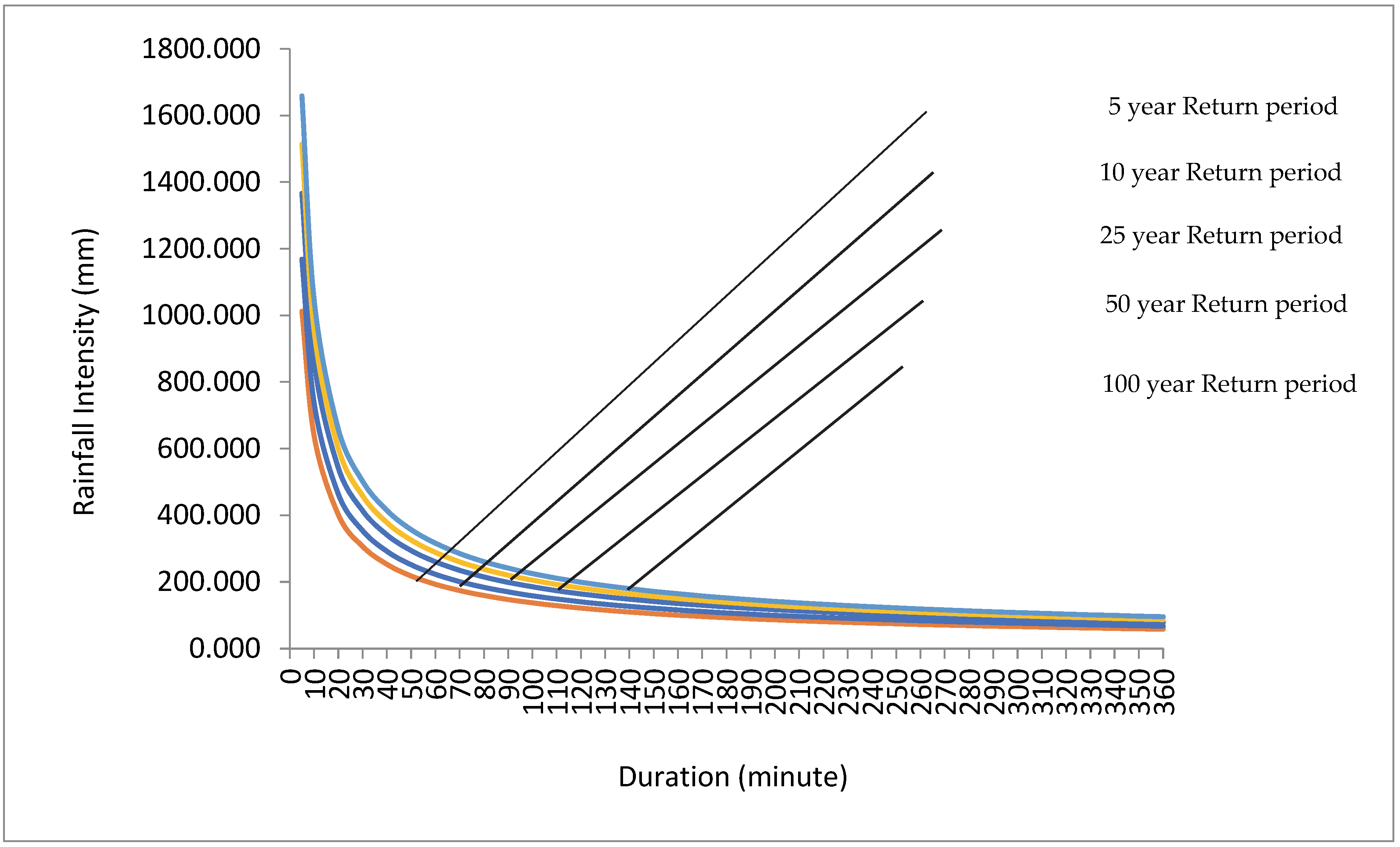
By using the Mononobe formula and rainfall design with the Log-Pearson Type III distribution, the rainfall intensity is shown in the table below [11].
Using the results of the rainfall analysis, which produces rainfall intensity with a return period (Table 4), we then created an IDF graph with the results, as shown in Figure 2.
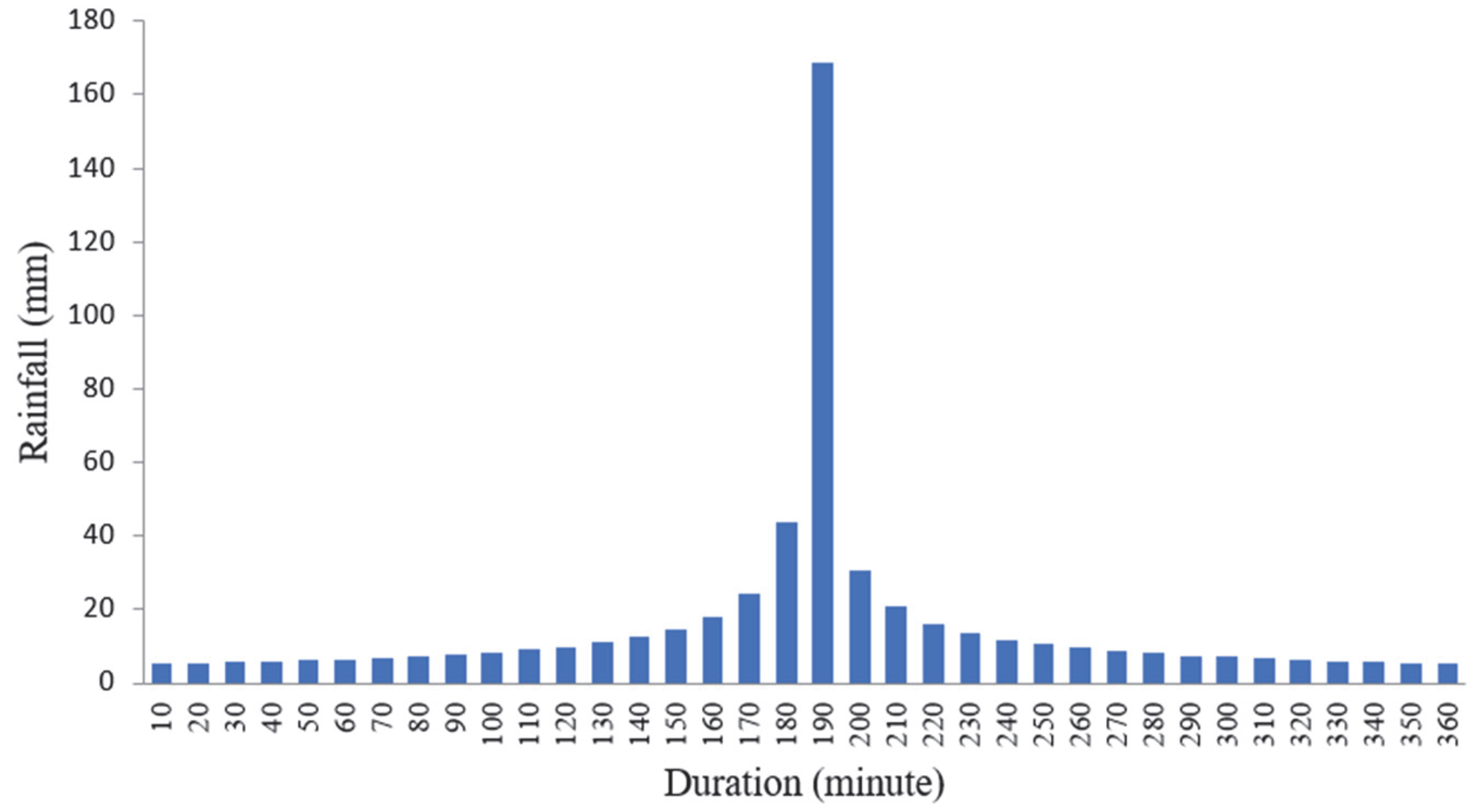
In calculating the design flood, input is needed in the form of design rain which is distributed into the hourly rainfall depth. In order to convert the design rainfall into hourly rainfall, it is necessary to obtain an hourly rainfall distribution pattern.
If what is available is daily rainfall data, to obtain hourly rainfall depth from design rainfall, a rainfall distribution model can be used. One of the rain distribution models developed to convert daily rain to hourly rain is using the Alternating Block Method (ABM) [11]. The results of the analysis were as shown in Figure 3.
4.4. Hydrodynamic Modeling Analysis
The results of hydrodynamic modeling are water level elevation, velocity, and several other hydraulic parameters. By performing this hydrodynamic modeling, the water level in each channel segment can be known so that segments that are not filled with water or overflow will be known.
With the knowledge of segments that are experiencing water shortages, the next step can be carried out, either by making reservoirs or by making channel improvements. Hydrodynamic modeling can also create plans/plans combined with control structures such as flood pumps and flood gates. Hydrodynamic modeling with HEC-RAS 2D can also compare plans between existing conditions and design conditions so that the design effect on changes in water level will be known [12].
The graphical facilities provided by HEC-RAS include X-Y graphs of river channels, cross-sections, rating curves, hydrographs, and other graphs which are X-Y plots of various hydraulic variables. HEC-RAS also provides a 3D plot feature of multiple latitudes at once. The model output results can also be displayed in tabular form. Users can choose between using tables provided by HEC-RAS or creating/editing tables as needed. Graphs and tables can be displayed on the screen, printed, or copied to the clipboard for inclusion in other application programs (word processor, spreadsheet) [13].
Along with this existing conditions modeling, simulation can also performed by not inputting from the source. This is intended to check whether the existing system can accommodate the burden of its watershed. The results of modeling the existing debit conditions and plan simulation conditions can be seen in Figure 4.
4.5. HEC-RAS Program
HEC-RAS is an application program for modeling river flow, the River Analysis System (RAS) created by the Hydrologic Engineering Center (HEC), which is a division within the Institute for Water Resources (IWR), under the US Army Corps of Engineers (USACE). HEC-RAS is a one-dimensional model of permanent and non-permanent flow (steady and unsteady one-dimensional flow model). The latest version of HEC-RAS, Version 4.1, has been in circulation since January 2010. HEC-RAS has four components of a one-dimensional model: (1) calculation of the water surface profile of permanent flows, (2) simulation of impermanent flows, and (3) calculations of sediment transport. An important element in HEC-RAS is that all four components use the same geometry data, the same hydraulic calculation routines, and several hydraulic design features that can be accessed after a successful water level profile calculation. HEC-RAS is an application program that integrates graphical user interface features, hydraulic analysis, management and data storage, graphics, and reporting [14,15].
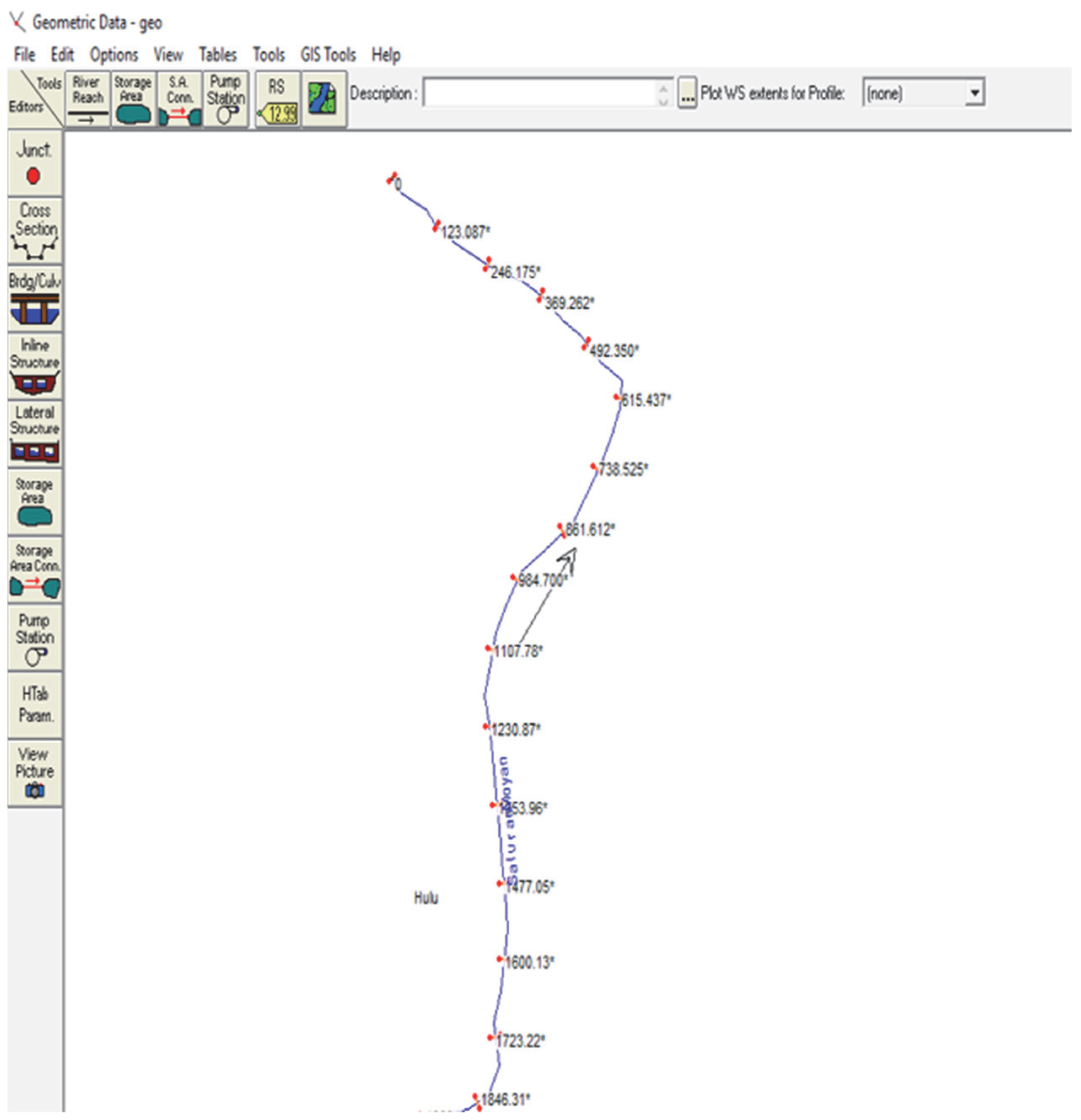
The HEC-RAS program is software used to analyze discharge where this software allows the user to perform one-dimensional steady flow, one and two-dimensional unsteady flow calculations, sediment transport/mobile bed computations, and water temperature/water quality modeling [16]. Figure 5 presents the Moyan Irrigation geometry menu in HEC-RAS software.
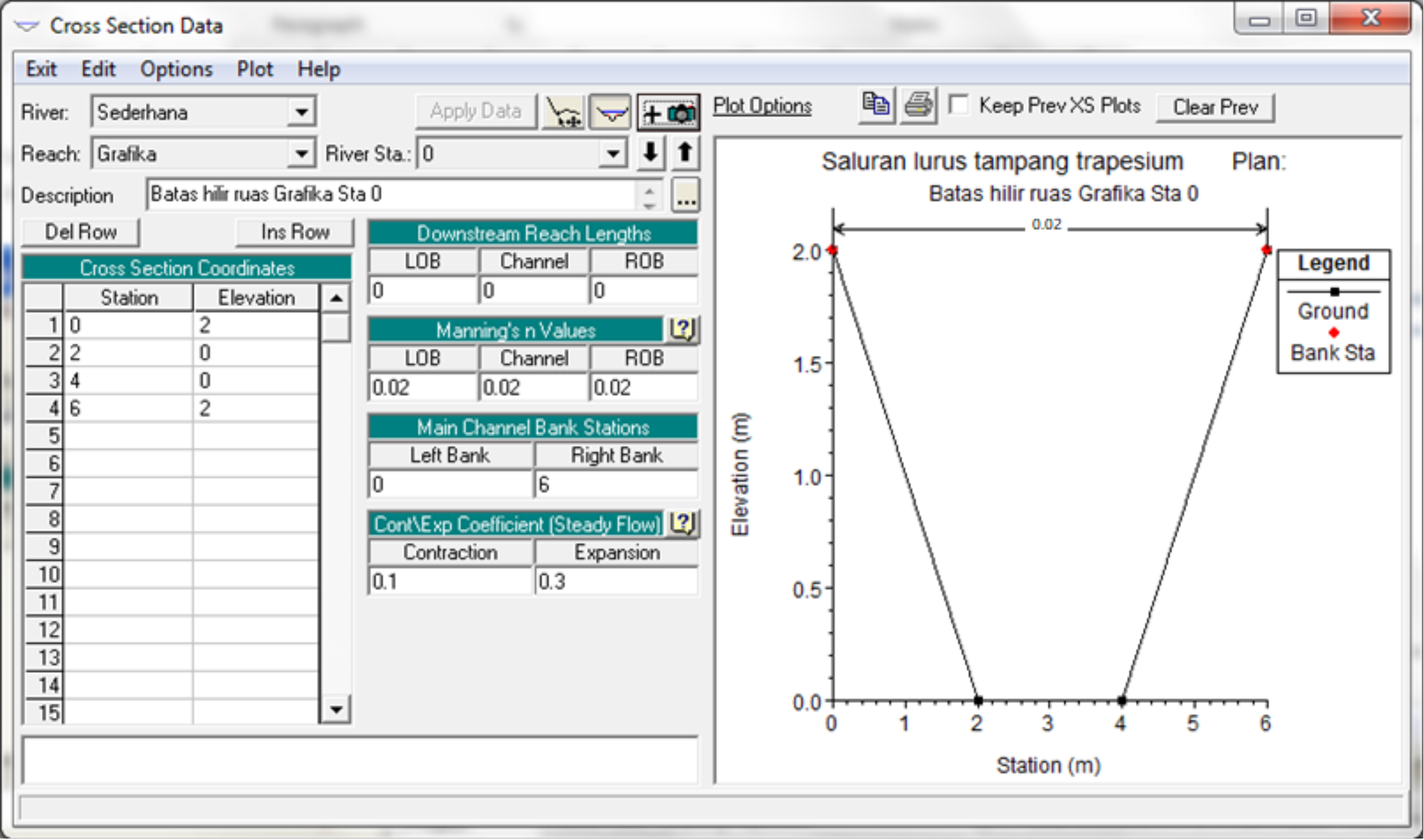
Cross Section Data
- The coordinates (Station, Elevation) of the latitude points on the River Sta are as follows: (0, 3), (2, 1), (4, 1), (6, 3). Remember, the base slope of the channel is 0.001 so the elevation at River Sta “1000” is 1 m above the elevation at River Sta “0” [18].
- Fill in the distance of the River Sta section “1000” to the downstream reach lengths with the number “1000” (the unit of length is meters), both for LOB, Channel, and ROB [19].
- Fill in Manning’s n Values, Main Channel Bank Stations, and Cont\Exp Coefficients do not need to be changed [20].
4.6. Data Input
Existing discharge was obtained from the measurement of the velocity with the current meter and water level from the bottom of the irrigation channel [21,22].
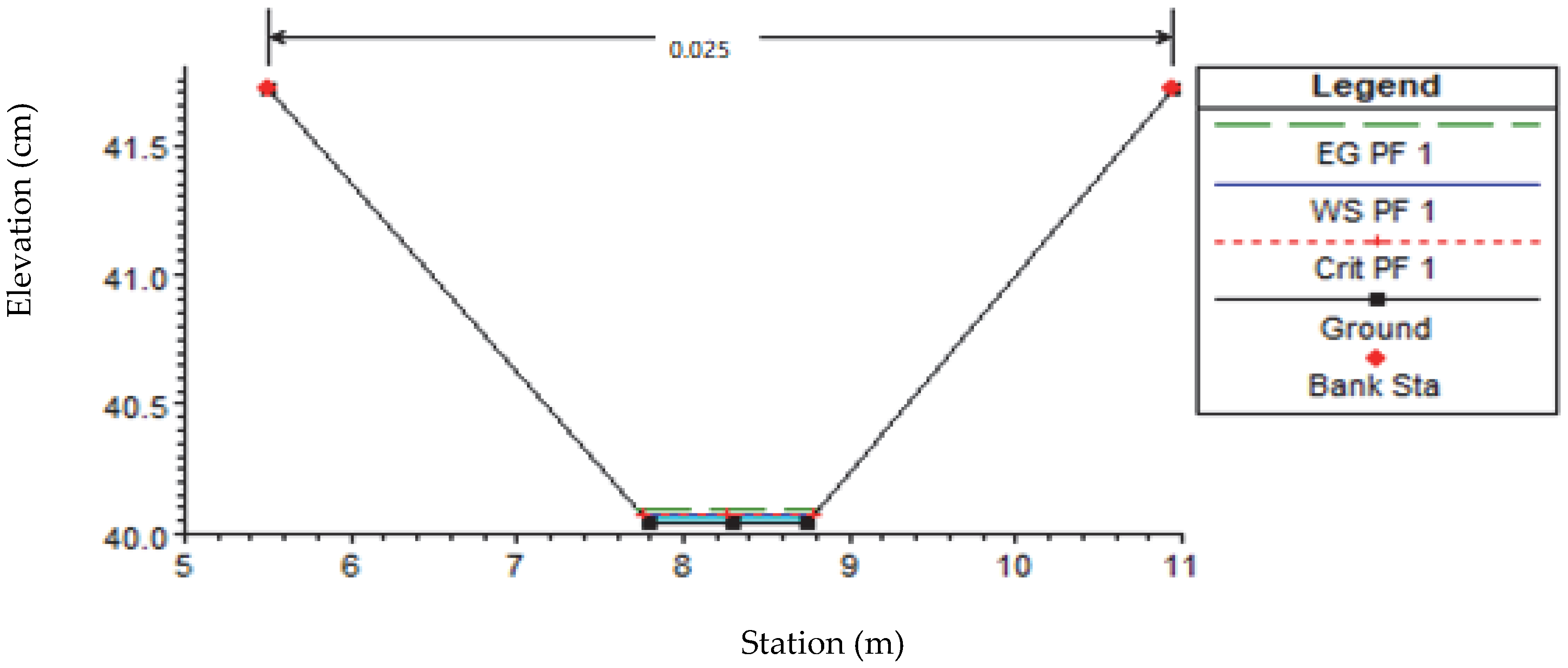
Figure 7 shows the river cross-section downstream with an existing discharge of 0.024 m3/s producing water height as high as 0.08 m.
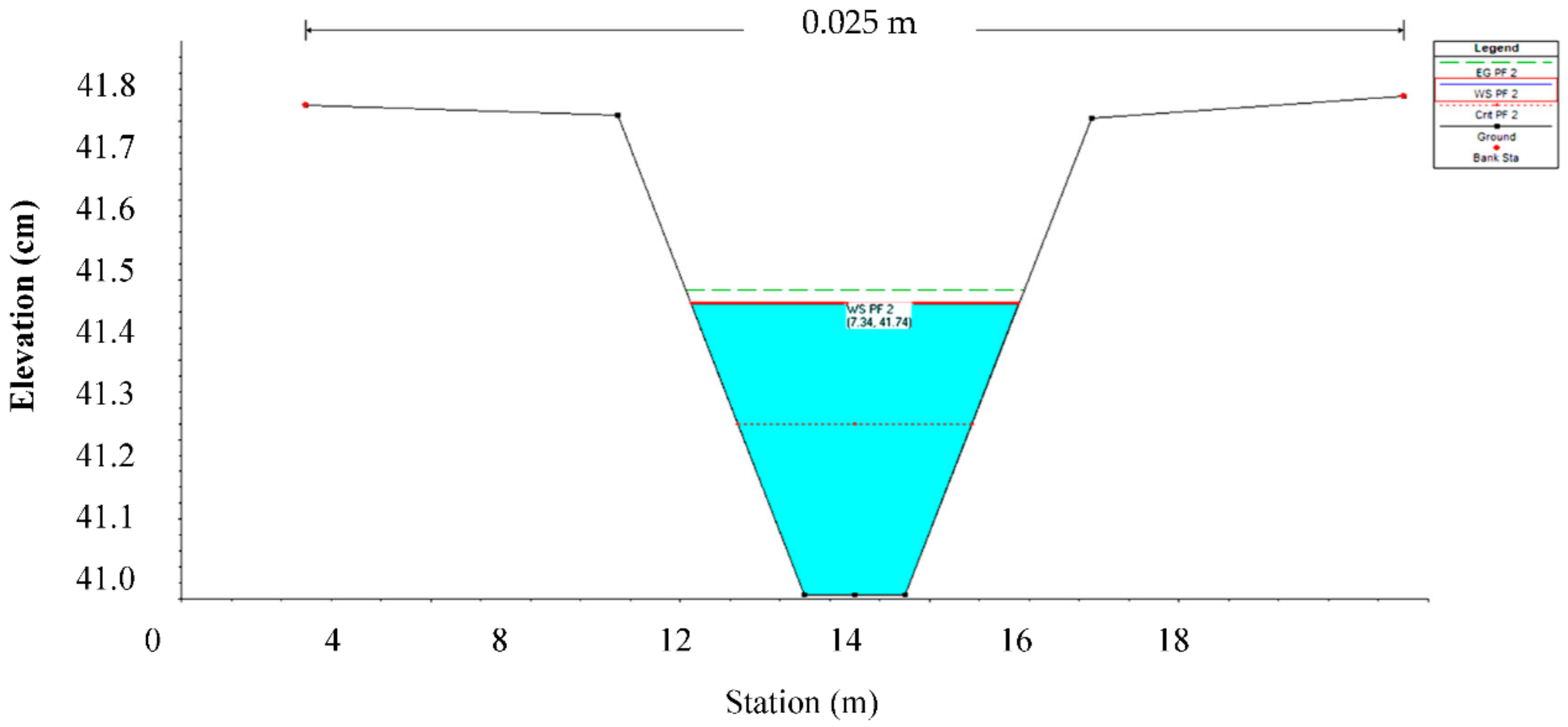
Figure 8 shows the river cross-section upstream with planned discharge 1 m3/s producing water height as high as 0.41 m.
Figure 9 shows the river cross-section downstream with a planned discharge of 1 m3/s producing water height as high as 0.404 m.
5. Conclusions
From this research, the following can be concluded:
- The Log-Pearson Type III distribution is the frequency distribution that matches the hydrological analysis in the research area. This method can be applied in analyses of river levels in other areas with heavy rainfall.
- The water level upstream and downstream is the same at 0.41 m with a discharge of 1 m3/s.
- The river cross-section downstream with the existing discharge of 0.024 m3/s produces water height as high as 0.08 m.
- With a flow rate of 0.783 m/s, the water level at the downstream cross-section is filled up to 0.75 m high, and the water level downstream of the irrigation channel is up to 0.40 m.
Author Contributions
A.S. (Alfrendo Satyanaga) and A.S. (Achmad Syarifudin) conceptualized the study; A.S. (Alfrendo Satyanaga) and H.R.D. implemented data processing under the supervision of A.S. (Achmad Syarifudin); the original draft of the manuscript was written by A.S. (Achmad Syarifudin) and H.R.D. with editorial contributions from A.S. (Alfrendo Satyanaga). All authors have read and agreed to the published version of the manuscript.
Funding
This research was supported by the Nazarbayev University Research Fund under Grant 11022021CRP1512.
Acknowledgments
The authors are grateful for this support. Any opinions, findings, and conclusions or recommendations expressed in this material are those of the author(s) and do not necessarily reflect the views of Nazarbayev University.
Conflicts of Interest
The authors declare no conflict of interest.
References
- The Republic of Indonesia Directorate General of Water Resources Ministry of Public Works and Housing. The Project for Assessing and Integrating Climate Change Impacts into the Water Resources Management Plans for Brantas and Musi River Basins (Water Resources Management Plan); Final Report, Volume II Main Report; Japan International Cooperation Agency, Nippon Koei Co., Ltd.: Jakarta, Indonesia, 2019. [Google Scholar]
- Rahardjo, H.; Satyanaga, A.; Harnas, F.R.; Leong, E.C. Use of Dual Capillary Barrier as Cover System for a Sanitary Landfill in Singapore. Indian Geotech. J. 2016, 46, 228–238. [Google Scholar] [CrossRef]
- Rahardjo, H.; Satyanaga, A.; Leong, E.C. Effects of rainfall characteristics on the stability of tropical residual soil slope. In Proceedings of the E-UNSAT 2016, E3S Web of Conferences, Paris, France, 9 September 2016; Volume 15004, pp. 1–6. [Google Scholar] [CrossRef] [Green Version]
- Syarifudin, A.; Satyanaga, A.; Wijaya, M.; Moon, S.-W.; Kim, J. Sediment Transport Patterns of Channels on Tidal Lowland. Fluids 2022, 7, 277. [Google Scholar] [CrossRef]
- CV Tata P’Setya. Final Report Assesment of River Discharge Data Air Lakitan Watershed; Department of Cipta Karya and Musi Rawas Regency Spatial Planning Public Works: Muara Beliti, Indonesia, 2017. [Google Scholar]
- Satyanaga, A.; Rahardjo, H. Unsaturated Shear Strength of Soil with Bimodal Soil-water Characteristic Curve. Geotechnique 2019, 69, 828–832. [Google Scholar] [CrossRef]
- Satyanaga, A.; Rahardjo, H. Stability of Unsaturated Soil Slopes Covered with Melastoma Malabathricum in Singapore. Geotech. Eng. 2020, 7, 393–403. [Google Scholar] [CrossRef]
- Ministry of Public Works and Public Housing of Indonesia. Law Number 7 Concerning Water Resources; Ministry of Public Works and Public Housing of Indonesia: Jakarta, Indonesia, 2004.
- Ministry of Public Works and Public Housing of Indonesia. Law Number 16 Concerning the Formation of the North Musi Rawas Regency; Ministry of Public Works and Public Housing of Indonesia: Jakarta, Indonesia, 2013.
- Syarifudin, A. Applied Hydrology; Andi Publishing Company: Yogyakarta, Indonesia, 2017; pp. 45–48. [Google Scholar]
- Yani, P.R.Y.; Saidah, H.; Wirahman, L. Hourly Rainfall Distribution Pattern at the Cliff Sate Rainfall Station and the Lingkok Lime Rainfall Station in the Central Lombok Region. Civ. Spectr. J. 2021, 8, 41–54. [Google Scholar] [CrossRef]
- Baitullah, A.A.M. HEC-RAS Short Tutorial for Beginners; Faculty of Civil Engineering, Sriwijaya University: Palembang, Indonesia, 2016. [Google Scholar]
- Istiarto. 1-D HEC-RAS Hydrodynamic Program Package for Basic Level of Flow Simulation: Simple Geometry River, Training Module; Springer Nature: Cham, Switzerland, 2014. [Google Scholar]
- Istiarto. Flood Inundation (HEC-GeoRAS), Technical Guidance; Istiarto: Yogyakarta, Indonesia, 2015. [Google Scholar]
- Syarifudin, A.; HRDestania, I.D.F. Curve Patterns for Flood Control of Air Lakitan river of Musi Rawas Regency. In the IOP Conference Series: Earth and Environmental Science, Proceedings of the 1st International Conference on Environment, Sustainability Issues and Community Development, Central Java, Indonesia, 23–24 October 2019; IOP Publishing: Bristol, UK, 2020; Volume 448. [Google Scholar]
- Syarifudin, A.; Destania, H.R. Water Overflow of the Riveranalysis Based on the Computerprogram Simulations (CPS); IAEME Publication: Palavakkam, India, 2020; Volume 11, pp. 125–136. [Google Scholar]
- Syarifudin, A. Environmentally Urban Drainage; Andi Publishing Company: Yogyakarta, Indonesia, 2017; pp. 38–42. [Google Scholar]
- Satyanaga, A.; Wijaya, M.; Zhai, Q.; Moon, S.-W.; Pu, J.; Kim, J.R. Stability and Consolidation of Sediment Tailings Incorporating Unsaturated Soil Mechanics. Fluids 2021, 6, 423. [Google Scholar] [CrossRef]
- Chua, Y.S.; Rahardjo, H.; Satyanaga, A. Structured Soil Mixture for Solving Deformation Issue in GeoBarrier System. Transp. Geotech. 2022, 33, 100727. [Google Scholar] [CrossRef]
- Satyanaga, A.; Rangarajan, S.; Rahardjo, H.; Li, Y.; Kim, Y. Soil Database for Development of Soil Properties Envelope. Eng. Geol. 2022, 304, 106698. [Google Scholar] [CrossRef]
- Li, X.; Wei, X.; Wei, N. Correlating check dam sedimentation and rainstorm characteristics on the Loess Plateau, China. Geomorphology 2016, 265, 84–97. [Google Scholar] [CrossRef]
- Satyanaga, A.; Bairakhmetov, N.; Kim, J.R.; Moon, S.-W. Role of Bimodal Water Retention Curve on the Unsaturated Shear Strength. Appl. Sci. 2022, 12, 1266. [Google Scholar] [CrossRef]
- Syarifudin, A.; Sartika, D. A Scouring Patterns around Pillars of Sekanak River Bridge. J. Phys. IOP Conf. Ser. 2019, 1167, 12019. [Google Scholar] [CrossRef]
- Yongmin, K.; Rahardjo, H.; Nistor, M.M.; Satyanaga, A.; Leong, E.C.; Sham, A.W.L. Assessment of Critical Rainfall Scenarios for Slope Stability Analyses based on Historical Rainfall Records in Singapore. Environ. Earth Sci. 2022, 81, 1–13. [Google Scholar]
Figure 1.
The location of the research works.

Figure 2.
Intensity Duration Frequency (IDF) Curve.

Figure 3.
Alternating Block Method (ABM) Log-Pearson Type III Distribution.

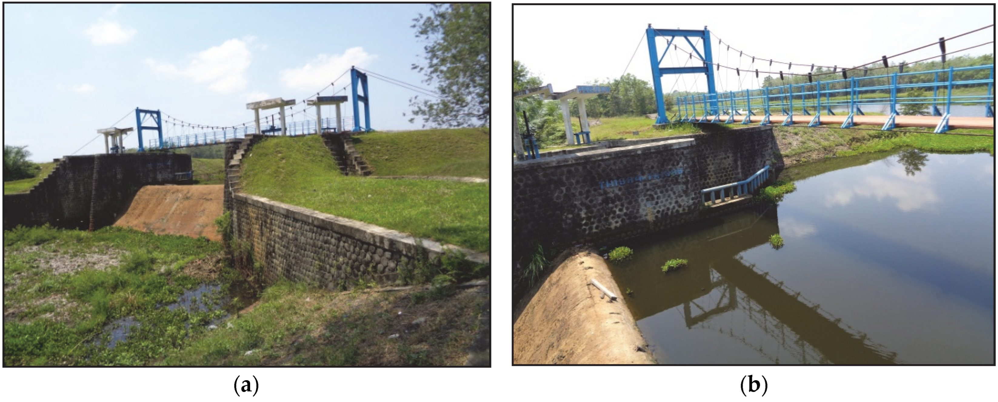
Figure 4.
(a) Downstream and water level of Moyan weir; (b) upstream of Moyan weir.

Figure 5.
Moyan Irrigation Geometry Menu.

Figure 6.
Cross section on the river.

Figure 7.
River cross-section downstream with existing discharge.

Figure 8.
River cross section upstream with planned discharge.

Figure 9.
River cross-section downstream with planned discharge.


Table 1.
Maximum rainfall data analysis result.
| Years | Rainfall (X) | LOG X | (X − Xaverage)2 | (X − Xaverage)3 | (X − Xaverage)4 |
|---|---|---|---|---|---|
| 1989 | 346 | 2.539 | 0.009 | −0.000805 | 0.000075 |
| 1990 | 448 | 2.651 | 0.000 | 0.000007 | 0.000000 |
| 1991 | 518 | 2.714 | 0.007 | 0.000556 | 0.000046 |
| 1993 | 441 | 2.644 | 0.000 | 0.000002 | 0.000000 |
| 1994 | 468 | 2.670 | 0.001 | 0.000055 | 0.000002 |
| 1995 | 417 | 2.620 | 0.000 | −0.000002 | 0.000000 |
| 1996 | 231 | 2.364 | 0.072 | −0.019358 | 0.005198 |
| 1997 | 298 | 2.474 | 0.025 | −0.003937 | 0.000622 |
| 1998 | 558 | 2.747 | 0.013 | 0.001502 | 0.000172 |
| 1999 | 365 | 2.562 | 0.005 | −0.000340 | 0.000024 |
| 2000 | 347 | 2.540 | 0.008 | −0.000773 | 0.000071 |
| 2001 | 626 | 2.797 | 0.027 | 0.004448 | 0.000731 |
| 2014 | 545 | 2.736 | 0.011 | 0.001134 | 0.000118 |
| 2015 | 417 | 2.620 | 0.000 | −0.000002 | 0.000000 |
| 2016 | 634 | 2.802 | 0.029 | 0.004910 | 0.007059 |
| Amount of data | 15 | ||||
| Amount | 39.482 | 0.113 | 0.0144 | 0.014118 | |
| Average | 2.632 | Cs | |||
| Standard of deviation | 0.090 | Ck |
Table 2.
Data Distribution of Requirements Testing for Using Frequency Analysis.
| Distribution Type | Terms | Calculation | Conclusion |
|---|---|---|---|
| Normal | Cs ≈ 0 | Cs = 1.9245 | No, fulfill |
| Ck ≈ 3 | Ck = 9.831 | ||
| Gumbel | Cs = 1.1396 | Cs = 1.9245 | No, fulfill |
| Ck = 5.4002 | Ck = 9.831 | ||
| Log Normal | Cs (ln x) = 0 | Cs (ln x) = −0.2133 | No, fulfill |
| Ck (ln x) = 3 | Ck (ln x) = 3.4689 | ||
| Log-Pearson Type III | Apart from top value | Cs = −0.2133 | Fulfill |
| Ck = 3.4689 |
Table 3.
Rainfall Design of the Log-Pearson Type III.
| T | P(%) | Cs | G | Log X | X (mm) |
|---|---|---|---|---|---|
| 2 | 50 | 0.2133 | −0.0373 | 2.0576 | 114 |
| 5 | 20 | 0.2133 | 0.8376 | 2.1894 | 155 |
| 10 | 10 | 0.2133 | 1.3117 | 2.2608 | 182 |
| 20 | 5 | 0.2133 | 1.7461 | 2.3262 | 212 |
| 25 | 4 | 0.2133 | 1.8329 | 2.3393 | 218 |
| 50 | 2 | 0.2133 | 2.1723 | 2.3904 | 246 |
Table 4.
Rainfall intensity.
| Tr (Year) | R24 (mm) | I (mm/h) |
|---|---|---|
| 5 | 114 | 45,0343 |
| 10 | 155 | 60,9973 |
| 25 | 182 | 71,8987 |
| 50 | 212 | 83,5867 |
| 100 | 218 | 86,1431 |
Note: R24 is rain for 24 h or 1 day.
Publisher’s Note: MDPI stays neutral with regard to jurisdictional claims in published maps and institutional affiliations. |
© 2022 by the authors. Licensee MDPI, Basel, Switzerland. This article is an open access article distributed under the terms and conditions of the Creative Commons Attribution (CC BY) license (https://creativecommons.org/licenses/by/4.0/).
Share and Cite
MDPI and ACS Style
Syarifudin, A.; Satyanaga, A.; Destania, H.R. Application of the HEC-RAS Program in the Simulation of the Streamflow Hydrograph for Air Lakitan Watershed. Water 2022, 14, 4094. https://doi.org/10.3390/w14244094
AMA Style
Syarifudin A, Satyanaga A, Destania HR. Application of the HEC-RAS Program in the Simulation of the Streamflow Hydrograph for Air Lakitan Watershed. Water. 2022; 14(24):4094. https://doi.org/10.3390/w14244094
Chicago/Turabian StyleSyarifudin, Achmad, Alfrendo Satyanaga, and Henggar Risa Destania. 2022. "Application of the HEC-RAS Program in the Simulation of the Streamflow Hydrograph for Air Lakitan Watershed" Water 14, no. 24: 4094. https://doi.org/10.3390/w14244094
Note that from the first issue of 2016, this journal uses article numbers instead of page numbers. See further details here.