Article

A Short Cost-Effective Methodology for Tracing the Temporal and Spatial Anthropogenic Inputs of Micropollutants into Ecosystems: Verified Mass-Balance Approach Applied to River Confluence and WWTP Release

1
Laboratoire Réactions et Génie des Procédés (LRGP), UMR CNRS 7274, Université de Lorraine, 1 Rue Grandville, 54001 Nancy, France
2
Laboratory of Materials, Catalysis, Environment and Analytical Methods, Faculty of Sciences I, Lebanese University, Campus Rafic Hariri, Beirut 1003, Lebanon
3
Luxembourg Institute of Science and Technology (LIST), 41 Rue du Brill, 4422 Belvaux, Luxembourg
4
Faculty of Science and Engineering, Maastricht University, P.O. Box 616, 6200 MD Maastricht, The Netherlands
*
Author to whom correspondence should be addressed.
Water 2022, 14(24), 4100; https://doi.org/10.3390/w14244100
Submission received: 4 November 2022 / Revised: 1 December 2022 / Accepted: 13 December 2022 / Published: 15 December 2022
(This article belongs to the Section Biodiversity and Functionality of Aquatic Ecosystems)

Abstract

:
The aim of this study is to develop a short cost-effective methodology for tracing the temporal and spatial anthropogenic inputs of micropollutants into ecosystems. The method involves a precise identification of the sampling sites based on various constraints: (1) one sampling site at each location to reduce the cost and the sampling time, (2) the sites are at sufficient mixing length from the release of micropollutants, and (3) they are identified with the aim to conduct mass balances. The methodology is applied to the identification, the quantification, and the distribution and transport of 21 emerging micropollutants in the Meurthe and Moselle river systems in the vicinity of the city of Nancy in France. The validity and reliability of the methodology is verified by using a mass-balance method at the confluence of the two rivers, where the mass fluxes upstream and downstream of the confluence compare well for nearly all the micropollutants. The methodology is employed to reveal mass fluxes of micropollutants discharged from the WWTP into the river water and point out the high efficiency of the drinking water treatment plant. The approach provides new insight into the identification of the sources of micropollutants in the rivers and the effects of hydrological and anthropogenic factors. The spatial anthropogenic inputs of micropollutants are highlighted in particular situations where discrepancies in the mass balance take place.

Graphical Abstract

1. Introduction

Water pollution is considered to be one of the global environmental challenges of the 21st century [1]. Emerging contaminants are water pollutants that are not currently regulated or only recently regulated, and there exist concerns regarding their risk on human health and the environment [2,3]. The first review article on emerging contaminants in water was published in 2003 [4]. When these chemicals are present in water bodies at trace-level concentrations up to a microgram per liter (µg/L), they are called micropollutants [5]. The emerging micropollutants family is very large and complex. It includes pharmaceuticals, personal care products, steroid hormones, endocrine-disrupting chemicals, and many other compounds [6,7,8]. These groups of chemical pollutants are emphasized most because they are recently proposed for addition to the list of priority substances in surface water by the European Commission (EC) and are also emerging contaminants of concern by U.S. EPA regulations. They originate from anthropogenic, agricultural, and industrial activities reaching the environment through sewer leaking, surface runoff, industrial discharges, and wastewater treatment plants discharges [9]. These contaminants find their way into surface water, groundwater, and even drinking water [10,11]. They have been reported to be present in water bodies at ng/L to pg/L concentration levels [11]. For example, diclofenac contamination was reported at concentrations ranging from 1 ng/L to 10 µg/L in surface water and 1 ng/L to 10 ng/L in drinking water [12]. It was proved that the occurrence of some of them in water bodies cause short- and long-term toxicity to wildlife, such as disruption of endocrines systems, bioaccumulation in the environment, and carcinogenicity [13]. In the European Union Directive 2013/39/EU, the standards for a group of 45 pharmaceuticals were studied. In 2015, a first watch list of 10 compounds was created in Decision 2020/1161/EU (see Table S1 of the Supplementary Materials).
Many studies performed in Europe and the whole world highlight the presence of a large variety of micropollutants in different water compartments at relatively high concentration levels above the limits and regulations [14,15,16]. As an example, it appears that one of the main sources of micropollutants in surface water is wastewater treatment plants (WWTPs) [17,18]. Their removal in WWTPs is not complete. In addition, the WWTPs exhibit variable removal rates between the compounds [6,19] and even for the same compound. For instance, the removal efficiency varies from 0% to 81.4% for diclofenac, while it ranges between 0% and 62.3% for carbamazepine [20,21]. In certain cases, some treatment processes end with the formation of by-products with significant estrogenic and antimicrobial activity [22,23]. Then a lot of micropollutants remain untreated or partially removed in the WWTP effluents and are discharged into receiving waters.
Some methodologies for the measurement and analysis of the source and transport of micropollutants into rivers, lakes, ground water, WWTPs, and drinking water have already been developed. Some are based on mass-balance approaches based on the mass flux of micropollutants in different positions [9,24,25]. These methodologies have been extended to larger areas to understand the sources, the occurrences, and the transport of micropollutants in the rivers [8]. The approach has been also used to follow the transformation of micropollutants during environmental transport into rivers [26]. However, measuring the micropollutants in rivers is still considered a long complex process that needs a lot of samples to achieve the desired analysis and studies. Then, the methodologies to be followed are generally long and expensive. This was one of our challenges, to develop and use a method to make a minimum number of samples to make an analysis with minimum expense and length with good, valuable results.
In this study, the presence of 21 micropollutants in river water samples from the Meurthe and Moselle rivers around the city of Nancy in France is analyzed and quantified. The studied contaminants are composed of pharmaceuticals, personal care products, plastic additive, and perfluorinated compounds. A short, inexpensive, and practical methodology for tracing the temporal and spatial hydrological and anthropogenic inputs of micropollutants into this ecosystem is established and implemented. Mass-balance approaches, based on mass flux of micropollutants, are developed. They allow the verification of the proposed methodology’s accuracy by comparing the micropollutants’ mass fluxes downstream of the confluence to the sum of the mass fluxes upstream of the confluence. Moreover, to allow the taking of samples at only one single location on the river cross-section, a good mixing is needed (same micropollutant concentration on the cross-section of the river). Consequently, a minimum distance is needed between the location of the micropollutants’ release upstream and the sampling location. Different methods of mixing-length estimation are presented. The variability of the mass flows of micropollutants depending on time, season and weather is studied. Based on this, the impact of anthropogenic (social and industrialized) activities, as well as hydrologic factors, on the transport and the distribution of the micropollutants along the two rivers is evaluated. Water samples are collected from five different sampling sites on both rivers from four sampling events over 18 months. The efficiency of the wastewater treatment plant and the drinking-water treatment plant is evaluated. It is also employed to identify the sources of micropollutants in the rivers and the effect of hydrological and anthropogenic factors.

2. Sample Collection and Analytical Methods

River waters were collected from the two rivers, the Moselle River (A) and the Meurthe River (B), close to the city of Nancy in France. The Meurthe River is a tributary of the Moselle River. The confluence is close to Nancy. Figure 1 represents a map of the sampling zone with the rivers and sampling locations, and Table 1 lists the codes used to represent the two rivers, the sampling locations, and the codes for other terms used in the article. River A has a length of 545 km and a 28,286 km2 catchment area where the French part covers 15,360 km2. Epinal is one of the French cities located along river A. River B is the largest tributary of A with a 161 km length flowing in the northeast of France through Nancy city in the Lorraine region. It flows into river A at Pompey (A2) on the northern edge of Nancy. On the one hand, the A-B area considered here contains three cities. Nancy, the biggest of the area, has 25,7431 inhabitants when coupled to its metropole that is constituted of 20 urban communities. Toul is a rather smaller city with 15,580 inhabitants. The city of Epinal is not reported on the map; it is located upstream 52 km from Messein (A1) along river A; 30,861 inhabitants live in this city.
On the other hand, the studied area has a wastewater treatment plant (WWTP) and a drinking-water treatment plant (DWTP). The WWTP of Nancy is located on river B. It treats wastewater with a capacity equivalent to 300,000 inhabitants for treatment of all the wastewater of the 20 communes of Nancy city. It uses different treatments such as screening and de-oiling, as well as an innovative biolift treatment developed by NANCIE, the International Water Center. The DWTP catchment is based along river A. The water is pumped in A1 on river A.
In this study, the water samples were taken from five different sites located on the two rivers (Figure 1 and Table 1). The positions of the sites were chosen to validate the mass-balance approach at the confluence of the two rivers, to investigate the release of the WWTP and the DWTP, and also to assess the anthropogenic inputs that are due to the cities of Nancy and Toul. The sampling site of Belleville (A3) is situated on river A downstream of the confluence of the two rivers A and B. Upstream of the confluence are located the sites of Moulin Noir (B2) on river B while Pompey (A2) is on river A. The sampling site of Malzéville (B1) is situated close to Nancy. More particularly, it is upstream of and very close to the WWTP (530 m). The comparison of the mass fluxes in B1 and B2 allows us to investigate the efficiency of the WWTP toward micropollutants. In the same vein, A1 is the place of the water catchment of the DWTP. In addition, drinking water obtained from the tap of the LRGP laboratory in Nancy is used to evaluate the efficiency of the DWTP. Four sampling campaigns were performed over two years (on 11 September 2015, 5 January 2016, and 14 October 2016). The samplings were conducted in all the sites that allow studying the seasonal and anthropogenic conditions. To cover all the seasons, an additional sampling was performed on 17 March 2017 only from B2. Two drinking-water samples from the LRGP laboratory in Nancy were sampled twice in January and October 2016. The weather conditions are presented in Table S2.
Twenty-one micropollutants from different classes including pharmaceuticals (Phs), endocrine disruptors (EDC), personal care products (PCPs), and some perfluorinated compounds (PFCs) were investigated. The list of the target compounds is presented in Table 2 with some data regarding the quantification and analysis. The selection of these micropollutants was based on various factors such as the usage (pharmaceuticals, hormones, and industrial compounds), the occurrence in the municipal wastewater, water systems, and different physical–chemical properties.
The samples taken were filtrated and preserved under the proper conditions. Then, they were extracted by offline solid-phase extraction (SPE) using an Auto-Trace SPE Workstation (Thermo Fisher Scientific, Waltham, MA, USA), based on the procedures explained in our previous works in detail [27,28]. The initial samples were concentrated with a ratio of 1000, and final volumes of 0.5 mL were kept at −20 °C until quantitative analysis. The SPE recoveries for each compound are listed in Table 2. After this step, the final extract was analyzed by liquid chromatography (1260 Series, Agilent, Santa Clara, CA, USA) coupled to triple-quadrupole mass spectrometry (QTRAP 4500, AB Sciex, Framingham, MA, USA). The chromatographic separation was achieved on a Zorbax Eclipse Plus C18 column displaying the following characteristics: 150 × 2.1 mm ID and 3.5 µm particle size (Agilent). The flow rate of the mobile phase was kept constant at 0.25 mL/min while the oven was maintained at 40 °C. The nature of the mobile phases and the eluent programs are given in Table S3 of the Supplementary Materials. According to the target compounds, the mass spectrometer was operated in positive or negative electrospray ionization (Table 2). The MS/MS was operated in multiple reaction monitoring (MRM) mode. Two MRM transitions were used for each compound of interest for quantification and confirmation. Quantitative results were provided thanks to the internal calibrations shown in Table 2.

3. Materials and Methods Developed

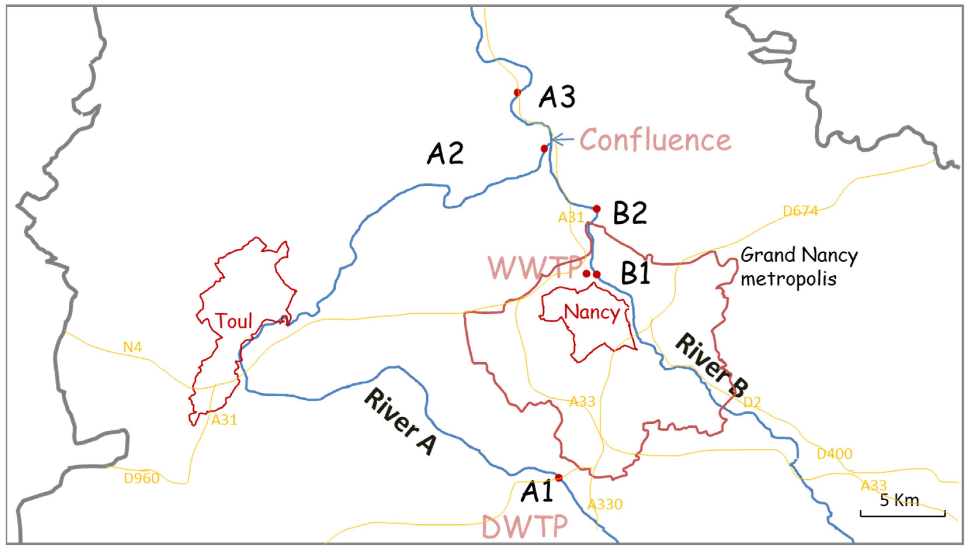
3.1. Objective and Constraints of the Sampling Zones
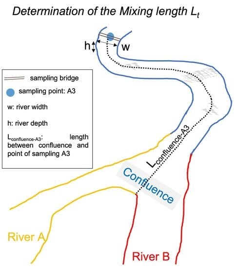
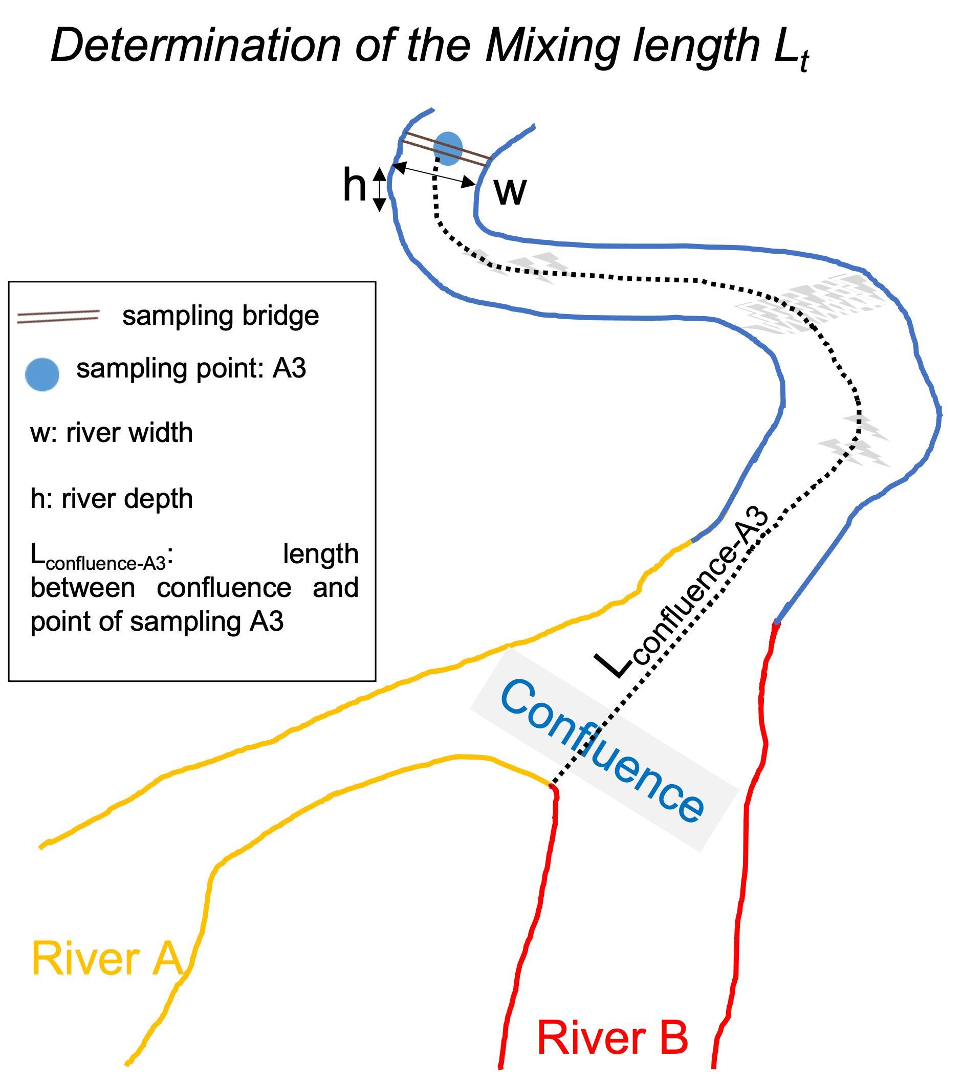
The choice of the sampling zone is very important. It was driven by several objectives and constraints. The aim was to conduct only one sampling at each site from only one position. For this, it was necessary to ensure that the micropollutant concentration was the same everywhere in the river section. Samples at each site were collected from only one sampling point in the middle of the bridge (which is in the middle of the river far from bridge pillars) to reduce cost. This served also to ensure the good mixing of the water content. The samples were collected using brown glass bottles surrounded by iron covers to avoid its breakage, using a thick long ribbon that was dropped from the bridge into the river to take the water samples. Samples were placed in 1 L dark glass bottles and transported to the laboratory. For being representative, the measured concentration should be the same everywhere on the river section. Then, there is a need for a sufficiently long distance between the sampling point and the last release of micropollutants (WWTP, brook, or confluence with another river). This distance is called “Mixing length”. It allows a good mixing of the two joined streams upstream (the river and the other stream carrying micropollutants, whether from a WWTP or another river) so that the micropollutant at the sampling point becomes uniformly distributed over the whole river cross-section, and then its concentration is constant over this cross-section. It was then necessary to estimate accurately this mixing length.

3.2. Mixing Length

Turbulent flows can be separated into two complementary flows: the advective flow that is related to mean velocity of the flow and the diffusive flow caused by its fluctuating components. This global diffusion is often called dispersion. This is modeled by Equation (1) for an infinitesimal volume of the river for a conservative flow (no transformation reactions):
u C i x D 2 C i x 2 + C i t = 0
where Ci is the concentration of micropollutant i in the elementary volume, t the time, u the river water velocity, x the unity of length along the river, and D the dispersion coefficient.
The dispersion is composed of three components at three different diffusion scales. The molecular diffusion, happening at the scale of the molecules, is due to Brownian movement. Molecular diffusion is very small compared to the two other diffusion processes, and then that is negligible in our configuration of rivers. The second component is the turbulent diffusion, also called eddy diffusion. The turbulence is characterized by the fluctuating component of the instantaneous velocity of the fluid particles. This mixing is due to eddies that happen at a wide range of scales from almost the scale of the river to the Kolmogorov microscale. It is an important process for the global diffusion (dispersion) in rivers. Finally, the differential advection can be due to the nonuniform advective flows (nonuniform velocity distribution) that are the consequence of the natural streams that possess different velocity gradients in horizontal and vertical directions [29].
As for molecular diffusion, there are diffusion coefficients for turbulence and dispersion, namely the turbulent diffusion coefficient and dispersion coefficient. The latter could be also called the axial dispersion coefficient. It is necessary to determine the mixing length that is the minimum distance on the river between the spread of pollutants and the location where the concentration of these pollutants can be considered the same over the whole width of the river. This ensures a good sample for measuring a micropollutant, since its concentration is the same over the whole width of the river, and then only one sample location is necessary in the middle of the river stream.
Dispersion coefficient could be measured by tracing experiments. Then different authors proposed correlations to determine it and to calculate the mixing length. Often, some authors propose a single dispersion coefficient to model the diffusion in a river; other authors propose two coefficients: a vertical dispersion coefficient and a transverse (or lateral) dispersion coefficient. In this case, two mixing lengths must be calculated and the longest should be chosen. The U.S. EPA describes in its report [30] the transverse mixing length Equations (2) and (6) (the necessary distance from the location of the confluence to obtain a perfect transverse mixing, i.e., the same concentration along the whole river width) using the transverse coefficient and shear velocity represented in Equations (3) and (4), respectively.
Actually, the authors used different equations, but they can be described as follows: the transverse mixing length Lt can be obtained from the velocity of the river flow U, the river width w, and the transverse dispersion coefficient Dt. The general form of Lt is generally given by:
L t = C o e f   U   w 2 D t
where Coef refers to a coefficient that differs based on the various models used to estimate Lt. Similarly, the general form of the expression used to determine the transverse mixing dispersion coefficient Dt reads as:
D t = C o e f   h   u
where h denotes the river depth (m), u* the shear velocity (m/s), and Coef’ a coefficient that varies depending on the models employed. The shear velocity can be expressed as:
u = ( g h S ) 0.5
where g is the classical g-force (m/s2) and S the river slope. Finally, Dt can be rewritten as:
D t = C o e f   h 1.5   ( g S ) 0.5
Consequently, all the expressions of Lt found in the literature are of the same form of:
L t = C o e f   U   w 2 h 1.5   ( g S ) 0.5
where only the coefficient Coef″ is modified based on the approximations employed (Coef″ = Coef/Coef′). The various expressions resulting from the different equations are summarized in Table 3.
Table 3. Calculation of the transverse mixing length for confluence and for WWTP using the different methods and equations. Our study parameters: for Lt (confluence): U = 0.14 m/s, h = 2.5 m, g = 9.8 m/s2, S = 0.0008, w = 127.62 m; for Lt (WWTP): U = 0.081 m/s, h = 2.5 m, g = 9.8 m/s2, S = 0.00027, w = 127.62 m.
CoefCoefCoefModel EquationLt (Confluence) (km)Lt (WWTP) (km)References
0.40.60.667 L t = 0.667   U   w 2 h 1.5   ( g S ) 0.5 4.32.1[30,31]
0.1250.160.78 L t = 0.78   U   w 2 h 1.5   ( g S ) 0.5 5.02.5[29,32,33]
0.0750.230.33 L t = 0.33   U   w 2 h 1.5   ( g S ) 0.5 2.21.1[34,35,36,37]
0.07590.60.133 L t = 0.133   U   w 2 h 1.5   ( g S ) 0.5 0.90.4[38]
Note: based on the altitude difference between the confluence and sampling point divided by their distance. Altitude values from https://fr-fr.topographic-map.com/, accessed on 1 June 2021.
Using these different equations developed by the different authors, the mixing length corresponding to our case study is calculated (Lt) using the different models. The results are represented in Table 3. These values are compared to the chosen length distance between the different sampling sites in our study. First, we consider the distance between the confluence of the two rivers and the sampling point downstream of the confluence, which is equal to 5.02 km (Lconfluence-A3). The different equations of mixing length are of the same base; they differ in the coefficient that is related to the estimation factor of the diffusion coefficient. This resulted in variable values to estimate the minimum sufficient transverse mixing length, as shown in Table 3. The sufficient transverse mixing length Lt (confluence) ranges between 0.9 km and 5.0 km with an average of 3.1 km. A distance Lconfluence-A3 of 5.02 km can ensure good mixing, taking into consideration also the advantage of the presence of a bridge allowing the taking of samples from the middle of the river. The sufficiency of the distance chosen will be validated below by the mass-balance model applied upstream and downstream of the confluence. This average minimum distance is also taken into consideration when the sampling points were chosen for the WWTP and B2 where LWWTP-B2 measures 3.69 km. The calculated Lt (WWTP) values range between 0.4 km and 2.5 km (Table 3). Based on these two Lt values, the three sampling sites A1, A2, and B1 were chosen, i.e., the distance between each of these three sites and any previous upstream release (intersecting river, wastewater release, etc.) is higher than the Lt calculated.
We can also add small remarks for the special cases of narrow waterways. We need to sample at a distance from the last pollutant release where the concentration of the pollutant is the same in the whole vertical section of the river. In our previous modeling, we only considered the transverse mixing, but there is also a second process, which is the vertical mixing. This assumption is justified, since in a large river, complete vertical mixing is reached before complete transverse mixing, and then the mixing length to reach complete transverse mixing is much higher than the one to reach complete vertical mixing. Then, only the transverse mixing length is calculated. However, for narrower waterways, the two parameters can be of the same order, and for very narrow ones, the vertical mixing length can be the limiting process.
Among the authors we cited in this article, Elhadi et al. [29] and Socolofsky and Jirka [38] also proposed two similar equations to model vertical mixing. The mixing length to reach vertical mixing can be written as follows:
L v =   K v U h 0.5 ( g S ) 0.5
However, the authors proposed two different Kv values: 1.79 for Elhadi et al. [29] and 1.19 for Socolofsky and Jirka [38].
To ensure that we reach the best mixing, we propose to use the highest Lv value, which is given by Elhadi et al. [29] with Kv = 1.79.
Then, for narrow rivers, the procedure would be to calculate Lv and Lt and to use the highest one. When the ratio Lt/Lv is lower than one, it is necessary to use Lv instead of Lt.
We can estimate the limit of the proportion of the waterway section (w/h) that separates the two domains where Lv or Lt is dominant.
Then, it is possible to compare them by the ratio Lt/Lv:
L t / L v =     K t U w 2 h 1.5 ( g S ) 0.5 / K v U h 0.5 ( g S ) 0.5
Giving:
L t / L v =     K t K v w 2 h 2
To ensure that we reach the best mixing, we propose to use the highest Lv value, which is given by Elhadi et al. [29] as Kv = 1.79. The same reasoning was previously applied to Lt in previous section, and again Elhadi et al. [29] gave the highest coefficient Kt of 0.78. Both values should be used to calculate the Lt/Lv ratio.
Using these parameters in Equation (9), we can calculate the proportion of the waterway section w/h that leads to two equals values for both the vertical and transverse mixing length. This situation occurs when:
L t / L v = 1               1 = 0.78 1.79 w 2 h 2
L t / L v = 1               w = 1.51 h
In conclusion, when the width (w) of a waterway is lower than 1.51 times its depth (h), the vertical mixing length should be used instead of the transverse one.

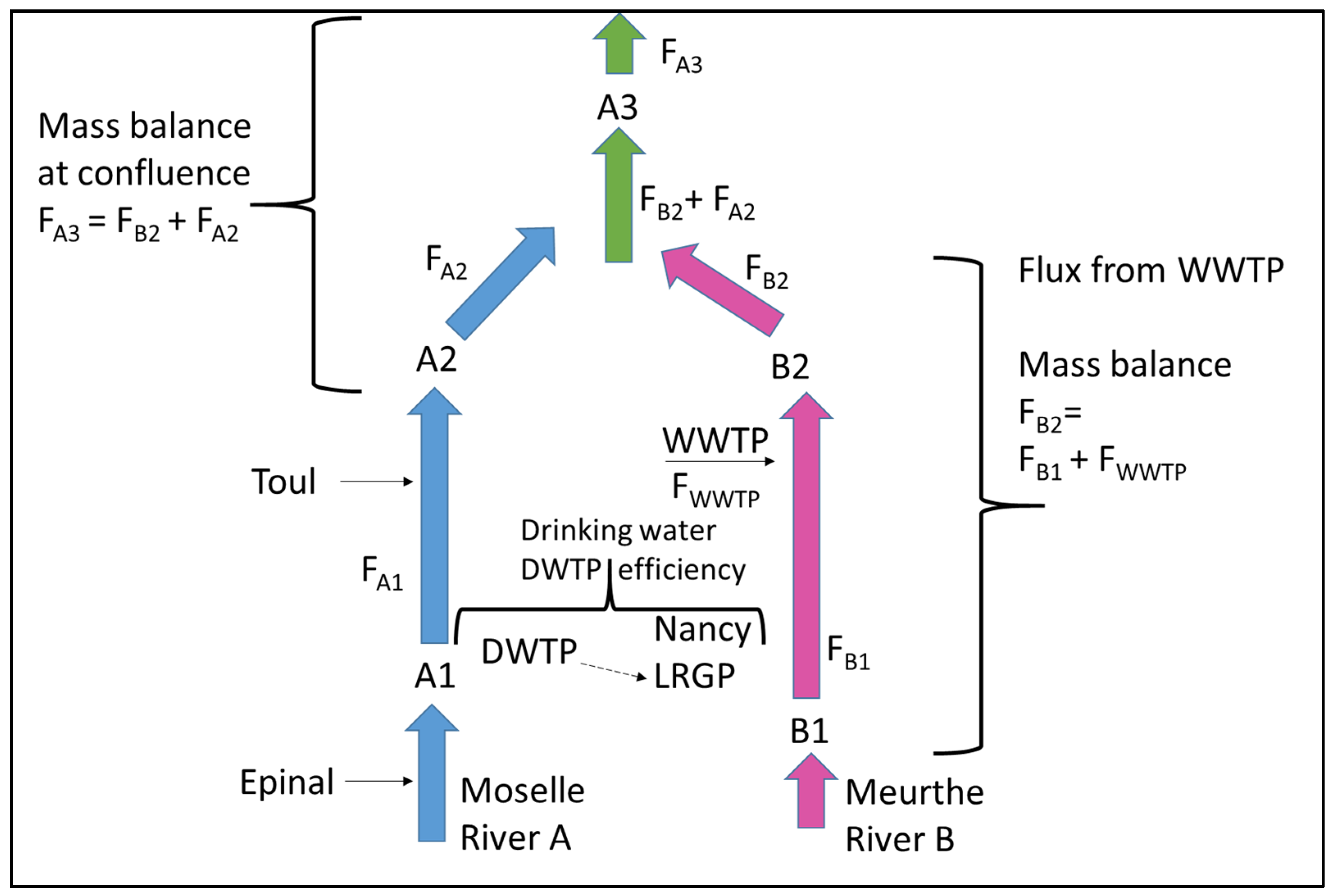
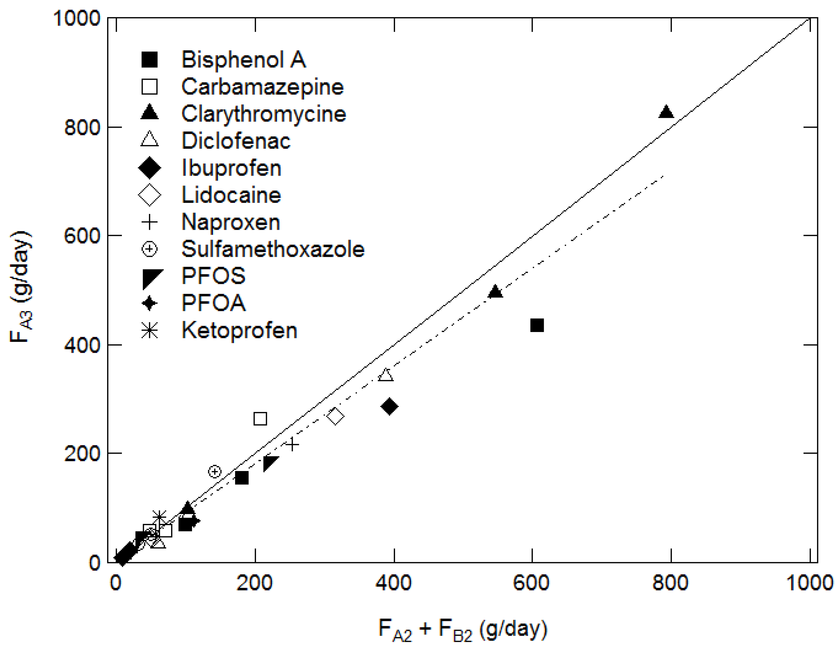
3.3. Verification of the Mixing Length Method by Using Mass Balance at a River Confluence

The flow rate data at each sampling site were provided by the “Ministère de l’écologie, du développement durable et de l’énergie” (site address: http://www.hydro.eaufrance.fr/, accessed on 1 May 2017). The values are presented in Figure S1 and also in Table S4 of the Supplementary Materials. The mass flux (Fijt) of each micropollutant i at location j and time t was calculated using the flow rate data (Q) and the concentration of the selected micropollutant (C) according to Equation (12).
F i j t = Q j t   C i j t
where Q is the river flow rate at the location j and time t, and Cijt is the concentration of micropollutant i at location j, time t of sampling.
Figure 2 illustrates the schematic representation of the rivers and the sampling sites with the corresponding flux of micropollutants. The zones where the mass balance was conducted are highlighted by brackets. In this part, the mass balance at the confluence is described to illustrate the development of the mass-balance approach. The mixing length is also discussed because it can impact the mass-balance results.
The mass balance at the confluence of rivers A and B is studied. More precisely, the mass flux of micropollutants from A2 and B2 is compared to that measured at A3. At the same time, the mass flux of river A downstream of the confluence should be equal to the sum of the two mass fluxes of the two rivers A and B upstream of the confluence:
F i   A d o w n s t r e a m = F i   A u p s t r e a m + F i   B u p s t r e a m
In our study, this mass balance is written as:
F i A 3 t = F i A 2 t + F i B 2 t
To validate the approach, the calculated mass flux upstream of the confluence, i.e., FA2 + FB2, is compared to the real flux downstream of the confluence at A3 represented by Fdownstream. The mass-balance precision percentage (fit%) for each micropollutant during a sampling day was defined by:
f i t % = F u p s t r e a m   F d o w n s t r e a m F u p s t r e a m × 100
Then, the average of fit% in the three sampling periods for each micropollutant was calculated using its absolute value according to Equation (16).
Average   f i % = | f i September % + f i January % + f i October % | 3
The study of the mass balances upstream and downstream of the confluence of the two rivers can be a way to control the quality of the measurements. For this goal, based on Equation (13), the agreement between the sum of the fluxes upstream of the confluence and the flux downstream of the confluence is represented in the scatterplot in Figure 3. The data points, for the various micropollutants and periods, fall on a single line close to the straight-line y = x, indicating that FA3 increases linearly with FA2 + FB2 (dotted line in Figure 3). The results highlight the good agreement between the sum of the fluxes upstream and the flux downstream of the confluence where the data fits with a high regression coefficient (R2 = 0.957). The slope of the line of the best fit to the complete dataset is 0.898. With respect to a perfect correlation, the slope would be 1 (see solid line in Figure 3). However, the slope of the averaged experimental straight line (0.89) is within the confidence range of the measurements. Some discrepancies are observed for some points, greatly for bisphenol A and less for ibuprofen. Not considering these two compounds, the correlation coefficient would be R2 = 0.9795. These points are related to the mass flux values in January when the flow rate is very high.
It appears that the studied compounds are of different concentration ranges (from a few ng/L to hundreds of ng/L), and thus of different mass flux measurement scales, i.e., Fupstream(PFOA) = 6 g/day while Fupstream(Clarithromycin) = 793 g/day. Consequently, it is not enough to validate the mass-balance approach by only comparing globally the fluxes upstream and downstream of the confluence. For this reason, the mass-balance precision percentage (fit%) and, more particularly, the average mass precision factor (average fi%) are used to evaluate the deviation from the mass balance for each compound when three values are available. The values are presented in Table 4 in increasing order of the average fi% values. The absolute values of the mass-balance precision percentage range between 6.3% as a minimum and 24.3%. The fit% values remain below 25% in the cases when it is possible to calculate an average for three sampling periods. As for the average fi%, it is mostly below 25% and even below 12% for the first four compounds. Such values remain relatively good, taking into consideration the difficulty of quantifying at the very low concentration of ng/L. For instance, PFOA has a concentration range between 2 and 5 ng/L in October. In addition, the percentage error of the chemical analysis is comprised of between 10% and 20%. Thus, the mass-balance approach is validated and it demonstrates the good quality of the measurements, as well as their precision and reliability. However, we need to take precautions when analyzing the mass flux and mass balance with some compounds such as diclofenac, ketoprofen, and PFOA.
Concluding on this, the validation of the mass-balance approach at the confluence verifies the mixing length method developed. It confirms that the distance taken between the confluence and the following sampling location (B3) is sufficient to ensure perfect mixing between the two rivers.

4. Results and Discussions

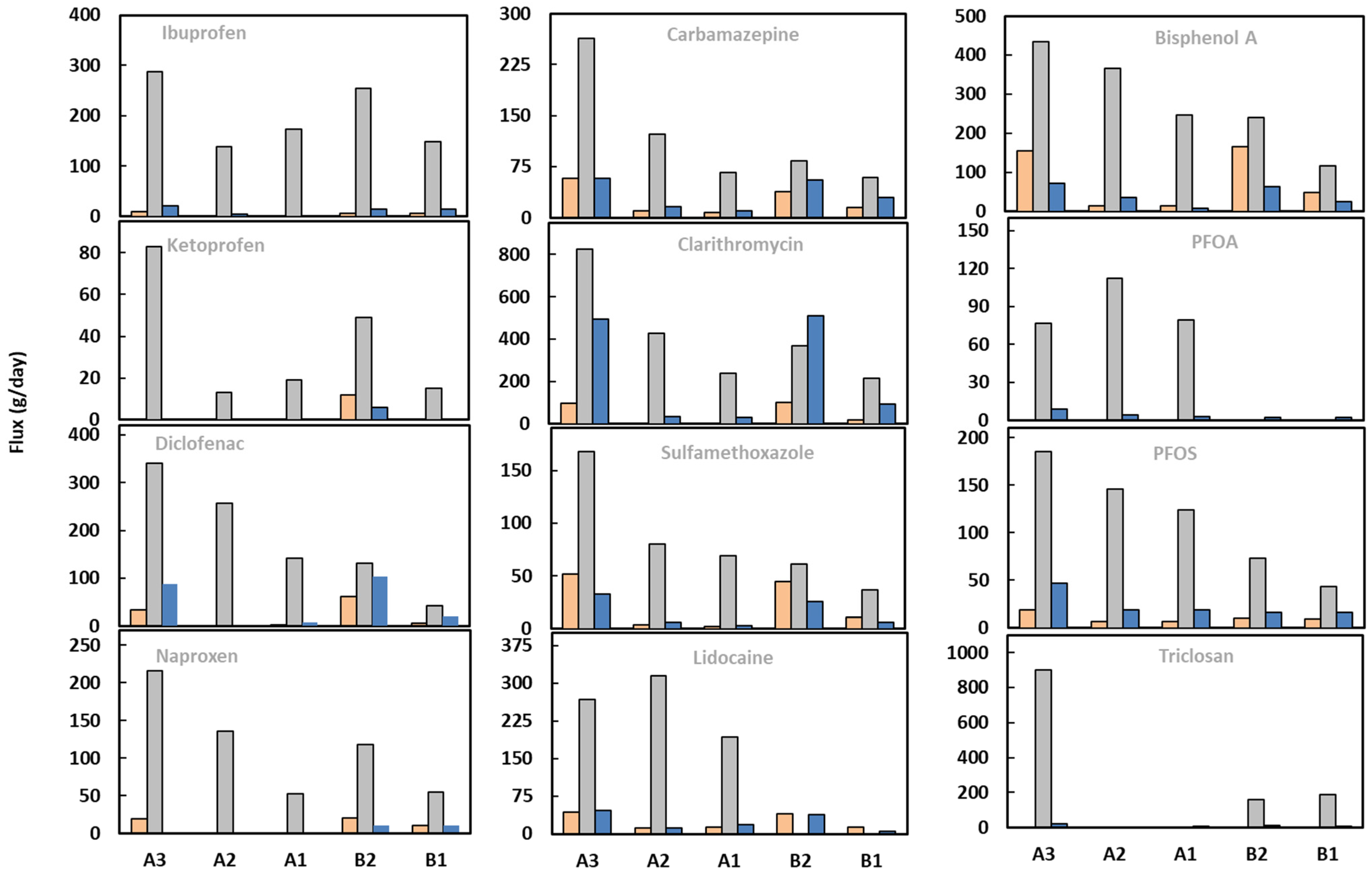
4.1. Overall Study of the Results

Out of 21 micropollutants, 16 compounds were detected in the river water samples. The concentration and mass flux of each compound, and the flow rate during the three sampling periods at the studied sites, are presented in Table S4 of the Supplementary Materials. The concentrations of the micropollutants ranged from a few ng/L to hundreds of ng/L. For example, diclofenac was detected in the measured samples at concentrations ranging from below the LoQ of 5.09 ng/L to 129 ng/L. The micropollutants concentrations were impacted by the type of the micropollutants, the location, and the period of the year. As general trends, the highest concentrations were reported in B2 while the lowest were detected in A1. Concerning the period of the year, the largest micropollutant concentrations occurred in October. As far as the nature of the micropollutants is concerned, the highest concentration was measured for the antibiotic clarithromycin with 639 ng/L in October (and 140 ng/L in January) in B2. It was followed by bisphenol A (236 ng/L in September, and 80–90 ng/L in January and October) and the two anti-inflammatory drugs diclofenac (129 ng/L in October, as well as 80 ng/L in September and 50 ng/L in January) and ibuprofen (97 ng/L in January), all measured in B2. Regarding the other micropollutants, the carbamazepine reached concentrations of 68 ng/L in October and 54 ng/L in September, sulfamethoxazole 64 ng/L in September, triclosan 59 ng/L in January, and lidocaine 57 ng/L in September—still in B2. Note that all these pollutants (except triclosan) were quantified in all the locations and periods. Erythromycin was quantified only in October with relatively high concentrations ranging between 260 ng/L and 900 ng/L, while its concentration was below the limit of quantification (LoQ) in September and January. This wide gap in the quantified concentration was also reported in other studies and was possibly due to the instability of the erythromycin molecule in solutions during the analysis and the storage of the sample [39,40].
Regarding the other pharmaceuticals’ compounds, the concentrations of the three antibiotics, sulfadimethoxine, sulfadimidine, and sulfathiazole, were always below the LoQ. Among hormones, estrone was the only one quantified. Its concentration was below the LoQ in September. Conversely, its concentration was quantified, at B2 and B1 in January and at A3 and B2 in October, with relatively low concentrations (2.8–7.5 ng/L). The concentrations of the two other hormones, namely estradiol-beta and ethynylestradiol, were below the LoQ at all sites and for the three samplings periods. The only personal care product (PCP), triclosan, was not always quantified, with some concentrations below LoQ and the highest concentration at 84.3 ng/L. The perfluorinated compound PFOS was quantified in all sites in the three periods with the highest concentration measured at 34 ng/L. Even with such a low ng/L level, the concentration of PFOS was still above the EU Environmental Quality Standards (EQS) fixed at 0.65 ng/L. PFOA was not always quantified, having a maximum measured concentration of 15.7 ng/L.
The analysis of the concentrations discussed above shows the variation in the concentrations between the different compounds, and for each compound at different dates across the two rivers and on different sites. In addition, it is realized that the highest concentration for most of the compounds was measured in B2, and the lowest concentrations were quantified in A1 and A2. This indicates that the temporal and spatial variations in concentrations are under the effect of some hydrological events, anthropogenic activities, and other factors that are discussed in the following parts.

4.2. Release of Micropollutants from WWTP

The estimation of the possible mass flux of micropollutants from the wastewater treatment plant (WWTP) was conducted. The mass flux coming from the WWTP released into the city river was represented as FiWWTPt. It was calculated, based on the mass-balance model, using the mass fluxes upstream (B1) and downstream (B2) of the WWTP, as illustrated in Equations (17) and (18).
FiB2t = FiB1t + FiWWTPt
The outgoing mass flux of micropollutants from the WWTP can be expressed as:
FiWWTPt = FiB2tFiB1t
To check the validity of the mass balance, it is necessary to compare the distances between location B2 and the WWTP, as well as between B1 and the location of the previous upstream release or confluence, to the mixing length Lt. The mixing length obtained with the various equations are reported in Table 3. The Lt values range from 0.4 km to 2.5 km. These values are lower than the distances between the previous upstream release and B1, or B2 and WWTP, which amounted to 3.69 km. Consequently, the mass balance and our sampling methodology can be safely applied to evaluate FiWWTPt.
Table S5 of the Supplementary Materials shows the concentrations of the quantified micropollutants upstream (B1) and downstream (B2) of the WWTP during the three sampling periods. The concentrations of the different groups of micropollutants increase downstream of the WWTP, which indicates that some micropollutants are still persisting in the WWTP effluents discharged into the river. This emphasizes the relative inefficiency of the WWTP in the complete removal of the micropollutants because of the use of conventional treatments that are not specified for their removal. This can explain the increase in the concentration of micropollutants from B1 to B2.
Based on the above results, the mass fluxes released by the WWTP, expressed as FiWWTPt, are calculated using the methodology of the mass-balance model (Equations (17) and (18)). For all the micropollutants and periods, the flux downstream of the WWTP (FiB2t) remains larger than the flux upstream of the WWTP (FiB1t). The values are presented in Table S5. It appears that 47% to 74% of the micropollutants downstream of the WWTP can be sourced from the WWTP effluents. This indicates that the WWTP effluents can be considered as a potential source of the micropollutants in surface water. The difference in FiWWTPt values between the three sampling periods for the same compound and between the compounds is related mainly to the fluxes of micropollutants in the WWTP influents sourced from city consumption and probably less by the removal percentage of each micropollutant in the WWTP. The seasonal variation of the mass fluxes and concentrations will be explained in Section 4.5.
To study the removal of micropollutants in the WWTP, the FiWWTPt and mean FiWWTPt for each micropollutant for the three sampling periods (average FiWWTPt) were used (Table 5). The highest FiWWTPt was measured for clarithromycin (average value of 218 g/day over the three periods). The obtained values are considered high (FiWWTPt = 84, 153, and 417 g/day). They are close to the values reported in three WWTPs effluents in Milan city in the range of 81–113 g/day [9], where relatively low removal percentages of mean value of 50% was obtained. Bisphenol A also displays high FiWWTPt with an average FiWWTPt of 93 g/day. This value is substantially larger than those reported by Castiglioni et al. [9] (12 g/day and 95% of removal efficiency) and Musolff et al. [41] (median WWTP effluent flux for bisphenol A of 40.5 g/day for 12 samples). The FiWWTP/inhabitant values are also calculated and presented in Table S5 since the release is highly affected by the population size of the cities corresponding to the WWTP present. It is then anticipated that bisphenol A is poorly removed in our WWTP. Diclofenac has also a high FiWWTPt with an average value of 76 g/day. This large value of the mass flux is probably due to the weak removal efficiency for this compound in the WWTP. A similar flux of 117 g/day coupled to a removal percentage of 28% have been reported by Castiglioni et al. [9].
Sulfamethoxazole has relatively moderate FiWWTPt (average value of 26 g/day). These values can be attributed to the poor removal efficiencies for this compound in the WWTP. Castiglioni et al. [9] reached the same type of conclusion since they reported a flux of 20 g/day and 17% of removal. The flux of carbamazepine also appears moderate with a value of 24 g/day. This value is well-comparable to what is reported in several studies where WWTP use conventional activated sludge treatment with chlorine disinfection [40] and biofilter-based treatment [9]. A removal of 83% is achieved under biofilter treatment. Naproxen, with mean FiWWTPt of 24 g/day, has a value close to that reported in one WWTP with 29 g/day effluent flux and 93% removal efficiency. The flux of ketoprofen also remains low (mean FiWWTPt value of 17 g/day). It is in close agreement to the effluent flux reported by Castiglioni et al. [9] with a high average removal percentage of 81%. PFOS has lower FiWWTPt in September and October (0–1 g/day), while it becomes high in January (30 g/day). Besides the high flow rates in January that explain the high flux values, the wide difference in the fluxes can be an indication for the fair removal in the WWTP. This phenomenon was also reported in many studies where the removal percentage reaches 50% as a maximum [9,42].
Estrone has low FiWWTPt of 9 g/day. This agrees well with the results obtained by Castiglioni et al. [9] (0.5 g/day and 90% removal) and Luo et al. [20] (removal 74.8–90.6%). This indicates that estrone seems to be efficiently removed in our WWTP. Ibuprofen has FiWWTPt of 1 g/day in September and October, while it is much higher in January (107 g/day). FiWWTPt of 1 g/day is close to what is reported in WWTP effluents with a removal of 99–100% [9] and another study with 72–100% removal [20]. The high FiWWTPt measured in January is due to the higher detected concentration of ibuprofen, which results from the greater use of this anti-inflammatory drug in winter against fever, pain, and flu, leading to high FiWWTPt. This can suggest that the mass flux and concentration of ibuprofen entering the WWTP are too large to be efficiently treated by the plant during this winter period.
Summarizing the results obtained, and by comparing our results to other studies, we can have an idea about the removal efficiency of our WWTP toward the studied micropollutants. Estrone, ketoprofen, naproxen, and ibuprofen seem to be efficiently removed. Conversely, clarithromycin, diclofenac, and sulfamethoxazole show weak degradation in the WWTP.

4.3. Drinking Water Assessment

Two drinking water samples from the LRGP laboratory located in Nancy, France, on January and October were analyzed. The concentrations of all the analyzed micropollutants CiDWt are below the limits of quantification. These concentrations are compared to the concentrations of micropollutants determined in A1 (Figure 2), which is the water catchment for drinking water (Table S6 of the Supplementary Materials). Referring to this table, 13 compounds that are present at quantified concentrations in the water from A1 are no longer detected in the analyzed drinking water with their concentrations below the limit of quantification. This reflects the efficiency of the drinking-water treatment plant (DWTP) for the removal of micropollutants at ng/L. After the treatment of the water by DWTP, it is used by the city for drinking and then goes to the WWTP for treatment before discharging it into river B. Consequently, most of the pollutants released in the rivers are coming from the activity of the city (some part is not removed by the WWTP), since the concentration of micropollutants in drinking water is below the LoQ.

4.4. Spatial Variations of Micropollutants in Rivers: Effect of Hydrological and Anthropogenic Factors

The concentrations of micropollutants in surface river water vary with the position from where the water samples are taken. The greatest concentrations are detected in B2 mostly, whereas the lowest concentrations are quantified in A1. B1 and B2 are located on river B, while A1 and A2 are situated on river A (Figure 1). The largest city in the region, Nancy, is located on river B. It corresponds to about 257,431 inhabitants. The water from the city is treated in a WWTP and released into river B between B1 and B2. The release of pollutants along river A is less since there are far smaller cities, Epinal with an average population of about 30,861 inhabitants and Toul with a 15,580 population. A1 has the lowest concentration for most of the micropollutants among all the other sites. As explained before, water from the A1 spot is pumped for appropriate treatment before being distributed to the city as drinking water. The weak concentration of micropollutants in A1 is a good indication of the quality of the water used for drinking.
Thanks to the mass-balance model based on the mass flux calculations, the concentrations of the micropollutants in the different sites can be explained and discussed. The fluxes from the cities (Nancy, Toul, and Epinal) are considered regardless of their sources (industries, domestic, etc.). We focus mainly on the number of inhabitants to explain the results. Figure 4 reports the mass fluxes of each of the quantified micropollutants at the different sites in the three sampling periods. The mass balance at the confluence (Equation (13)) predicts that the maximum mass flux of micropollutants is obtained at A3. This is experimentally confirmed for the majority of the micropollutants for the three sampling seasons. However, a large difference between the flow rates occurs between A3 and B2. Significantly higher flow rates Q3 are recorded in A3. As a consequence, since Cijt = Fijt/Qjt, the concentrations of micropollutants in B2 become larger than in A3. This corresponds well to the experimental results for which the greatest contaminant concentrations are recorded in B2. In this situation, it appears that the Meurthe River water (B2) was diluted by the Moselle River (A2).
Experimentally, it also appears that, in September and October, the mass flux of micropollutants in A2 is lower than that in B2. In other words, FiA2t << FiB2t. This applies for the majority of the micropollutants except for PFOS and PFOA. These two pollutants are discussed later. Using the mass-balance approach, the following equations can be utilized:
FiA2t = FiA1t + FiToult
while:
FiB2t = FiB1t + FiWWTPt
where the mass flux FiWWTPt is related to the mass flux released from the city of Nancy. This result can be explained by considering that the mass flux of micropollutants from Nancy is substantially larger than that from the small cities of Toul and Epinal. For the two periods, the flow rates in A2 and A1 are similar. Consequently, larger micropollutant concentrations are expected to be recorded in B2 most of the time.
On the river B side, it was already reported that the mass fluxes of micropollutants in B2 are higher than those observed in B1: FiB2t > FiB1t. This occurs for all the micropollutants regardless of the date of sampling. This was explained by the flux from Nancy and, more particularly, from the WWTP (FiB2t = FiB1t + FiWWTPt), based on Equation (17). Logically, the pollutant concentration is larger in B2 and is the largest among all the sampling sites studied.
On the river A side, it appears also experimentally that the mass fluxes of micropollutants in A2 exceed those reported in A1 for the majority of the contaminants (except for lidocaine in September and October, as well as ibuprofen and ketoprofen in January) and for the three samplings periods. This is explained through Equation (19), which indicates that FiA2t = FiA1t + FiToul. However, in terms of micropollutant concentrations, A2 is a little higher than A1.
Finally, the lowest mass flux of micropollutants is encountered in A1. This corresponds, for the majority of the micropollutants, for the three periods, to the weakest micropollutant concentrations. This is the reason why the water used as inlet source in the drinking-water plant is pumped from this position, after a long section called “Moselle sauvage” (literally “wild Moselle River”), a nature reserve with no pollutants release and where a self-purification process happens.
It seems relevant to discuss particular situations where discrepancies in the mass fluxes take place. As previously mentioned, for the two perfluorinated compounds, the mass fluxes seemed not to respect the proportion of inhabitants at the catchment. Actually, the fluxes of PFOA and PFOS in A2 appear much larger than those in B2 (FA2t (PFOA) >> FB2t (PFOA) and FA2t (PFOS) >> FB2t (PFOS)) in January and October. It can be also mentioned that for PFOA, the flux in river B is negligible (0–2 ng/L), while it reads as 112 ng/L in river A. This highlights an anthropogenic source of PFOA and PFOS in river A. A factory located on river A could be responsible for the release of the two perfluorinated compounds.
Another peculiar behavior can be outlined with triclosan. This micropollutant is only quantified in B1, B2, and A3. At the same time, it cannot be quantified in A2 and A1, i.e., along river A. This highlights an anthropogenic source of triclosan in river B released from the WWTP. It can be also pointed out that the mass flux increases significantly after the confluence at A3. This is another example where the mass balance does not loop since FA3t (triclosan) >> FA2t (triclosan) + FB2t (triclosan), which is the opposite of what is predicted by Equation (14). There is also probably a factory just upstream of A3 (between A2 and A3 or between B2 and A3). It shows another interest of such a mass-balance method, i.e., identification of hidden micropollutant release.
Erythromycin also displays a particular behavior. Its mass flux and concentrations are below LoQ in September and January in all sampling positions. Conversely, it becomes quantified only in October with relatively high concentrations ranging between 260 ng/L and 900 ng/L. In addition, this micropollutant does not respect the mass balances. As an example, at the confluence, FA3t (Erythromycin) << FA2t (Erythromycin) + FB2t (Erythromycin), which is in perfect disagreement with Equation (14). The sum of the mass fluxes in A2 and B2 is approximately two times larger than the mass flux in A3. This wide gap in the quantified concentrations was also reported in other studies and is possibly due to the instability of the erythromycin molecule in solutions during the analysis and the storage of the sample [30,39].

4.5. Temporal Variations of Micropollutants in Rivers

To discuss the effect of the sampling date on the release of the compounds, we focused on the concentrations of the micropollutants in B2 where the contaminant concentrations are the highest. It was possible to follow the temporal evolution of micropollutants over 18 months. The concentration of the micropollutants in B2 in September, January, October, and March are reported in Table 6. Several behaviors were encountered depending on the micropollutants type.
The pharmaceutical compounds ibuprofen, ketoprofen, and naproxen display the highest mass flux in January (winter season). These three drugs are non-steroidal anti-inflammatory drugs. They are specifically used to treat inflammation or pain caused by many conditions such as arthritis, menstrual cramps, bursitis, and tendinitis, which are more prominent in winter when people also suffer from joint pain, fever, and flu. In winter, ibuprofen has higher mass flux than the other two drugs. It is more commonly used by people, especially to reduce fever, headache, and back pain. Similar reasoning can be applied to triclosan, for which the largest release is observed in winter because of the higher consumption of products containing triclosan in that season. Soaps, first-aid kits, and hydroalcoholic solutions are examples of products containing triclosan.
The groups of micropollutants including diclofenac and carbamazepine have releases into rivers that are globally constant throughout the year, especially carbamazepine, which is a long-term treatment against epilepsy. Finally, clarithromycin displays a maximum mass flux in October and January. These drugs are used mainly in autumn and winter.

5. Conclusions

In this study, a short cost-effective methodology for tracing the temporal and spatial anthropogenic inputs of micropollutants into ecosystems has been developed. The method was based on an accurate selection of the sampling sites based on several constraints. The methodology involved sampling from only one position at each location to reduce the cost. The sampling was conducted from the middle of a bridge on each location (and far from bridge pillars). This can be done only if the sampling location respected the mixing length needed for sufficient mixing of micropollutants between the sources of release and the sampling positions. In other words, if this condition was not respected, i.e., if the distance between the sampling sites was lower than the mixing length, it became necessary to perform various samplings in different positions of the bridge for each sampling site. Moreover, there would be a need to identify the velocity profile in the river to calculate the fluxes, which would increase the cost of the method. The sampling sites were also identified with the aim of conducting mass balances based on the flux of micropollutants between the different sampling positions. A multi-residual analytical technique based on a preconcentration step using solid-phase extraction followed by liquid chromatography tandem mass spectrometry analysis (LC-MS/MS) was used. It allowed the detection and quantification of 21 emerging micropollutants in the Meurthe and Moselle river systems at a ng/L concentration level. With four sampling campaigns conducted during two years from five sites, the micropollutants were analyzed upstream and downstream of the confluence of the two rivers, upstream and downstream of a wastewater treatment plant, and from a drinking-water catchment.
The method was validated thanks to the mass balance applied at the confluence between the two rivers. At the confluence, the sum of the two mass fluxes upstream compares well with the values recorded in the sampling site downstream of the confluence for nearly all the micropollutants. An average mass-balance precision percentage (fit%) was mostly below 25% (range between 6% and 24%), which was considerably small. This revealed the validity and reliability of the methodology. This confirmed also the precision and the quality of the analytical protocol used for the measurements of the micropollutants at low concentrations.
Using this approach, the release of micropollutants from WWTP was evaluated with the aim to discuss their removal efficiencies. Mass fluxes were discharged from the WWTP into the river water, where their removal efficiencies seemed to vary between the compounds. Drinking water samples were also analyzed. The concentrations of all the micropollutants were below the limit of quantification. This emphasized the high efficiency of the drinking-water treatment plant of the city of Nancy, since the micropollutants measured at the site of A1, where the water was pumped prior to treatment, had significantly larger micropollutants content.
The methodology allowed the identification of the sources of micropollutants in the rivers and the effect of hydrological and anthropogenic factors. The approach explained successfully the spatial variation of the concentrations of the majority of the micropollutants in the different sites experimentally observed. The results were described based on the mass flux from the cities (situated on the whole catchment). The spatial anthropogenic inputs of micropollutants were highlighted in particular situations where discrepancies in the mass balance took place. The presence of some industrial factories was confirmed by the detection of high concentrations of some compounds. Human activities released micropollutants through domestic waste. They were affected by the consumption rate for several types of compounds that depended on seasonal variations, especially for pharmaceuticals. They were also impacted by some government regulations that put the limitations on the use of some compounds such as bisphenol A.
This study gives important information on the occurrence of micropollutants in the river water of the Meurthe River and the Moselle River in France. It highlights the different industrial and anthropogenic sources of microcontaminants. It provides useful information on the fate of micropollutants in the WWTP present in this region to update the plant with more efficient treatment methods for higher removal efficiencies for micropollutants. The results presented also provide a useful methodology for tracing the temporal and spatial hydrological and anthropogenic inputs of micropollutants into ecosystems. Future work will use this approach with other ecosystems.

Supplementary Materials

The following supporting information can be downloaded at: https://www.mdpi.com/article/10.3390/w14244100/s1. Table S1. The first watch list of the 10 compounds created in the Decision 2015/495/EU; Table S2. Weather conditions during the four sampling periods; Table S3. Parameters of the LC-MS/MS instrument, including mobile phases and eluent programs. The notation “min” corresponds to minutes; Table S4. The Concentrations (C) in ng/L and mass fluxes (F) in g/day for the 21 micropollutants in 5 sampling sites on 3 sampling dates; Table S5. The concentrations (ng/L), mass fluxes F (g/day), flux FiWWTPt (g/day) and flux FiWWTPt per inhabitant (g/day.Inhabitant) of the quantified micropollutants upstream and downstream the WWTP during the three sampling periods. The sum represents the sum of the mass fluxes for all the micropollutants upstream WWTP and from WWTP, and the percentages are calculated with respect to the total sum downstream WWTP. The letter F refers to mass flux and C to concentration. A dash ‘-’ is used when Cit at the site is < LoQ; Table S6. Concentration of micropollutants in A1 on January and October; Figure S1. The variation of the flow rate during the three sampling periods at the five sampling sites.

Author Contributions

Conceptualization, O.P. and T.R.-C.; methodology, O.P., T.R.-C. and H.A.; sampling of water, H.A., S.P., H.P., O.P. and T.R.-C.; micropollutants measurements, H.A., A.L. and C.G.; formal analysis, O.P. and T.R.-C.; investigation, H.A., T.R.-C. and O.P.; resources, J.T., T.H., B.K., T.R.-C. and O.P.; data curation, H.A., T.R.-C. and O.P.; writing—original draft preparation, T.R.-C. and H.A.; writing—review and editing, H.A., T.R.-C. and O.P.; supervision, T.R.-C. and O.P.; project administration, T.R.-C. and T.H.; funding acquisition, J.T., T.H., O.P. and T.R.-C. All authors have read and agreed to the published version of the manuscript.

Funding

This research received no external funding.

Acknowledgments

We would like to thank the “Institut Carnot ICÉEL” for the support of the “STEP-Design project”.

Conflicts of Interest

The authors declare no conflict of interest.

References

  1. Liu, H.; Nkundabose, J.P.; Chen, H.; Yang, L.; Meng, C.; Ding, N. Decontamination of ibuprofen micropollutants from water based on visible-light-responsive hybrid photocatalyst. J. Environ. Chem. Eng. 2022, 10, 107154. [Google Scholar] [CrossRef]
  2. Gomes, I.B.; Simões, L.C.; Simões, M. The effects of emerging environmental contaminants on Stenotrophomonas maltophilia isolated from drinking water in planktonic and sessile states. Sci. Total Environ. 2018, 643, 1348–1356. [Google Scholar] [CrossRef] [PubMed] [Green Version]
  3. Kumar, R.; Vuppaladadiyam, A.K.; Antunes, E.; Whelan, A.; Fearon, R.; Sheehan, M.; Reeves, L. Emerging contaminants in biosolids: Presence, fate and analytical techniques. Emerg. Contam. 2022, 8, 162–194. [Google Scholar] [CrossRef]
  4. Richardson, S.D. Water Analysis: Emerging Contaminants and Current Issues. Anal. Chem. 2003, 75, 4943. [Google Scholar] [CrossRef] [Green Version]
  5. Stamm, C.; Räsänen, K.; Burdon, F.; Altermatt, F.; Jokela, J.; Joss, A.; Ackermann, M.; Eggen, R. Unravelling the Impacts of Micropollutants in Aquatic Ecosystems. In Advances in Ecological Research; Elsevier: Amsterdam, The Netherlands, 2016; Volume 55, pp. 183–223. [Google Scholar] [CrossRef]
  6. Gallé, T.; Pittois, D.; Bayerle, M.; Braun, C. An immission perspective of emerging micropollutant pressure in Luxembourgish surface waters: A simple evaluation scheme for wastewater impact assessment. Environ. Pollut. 2019, 253, 992–999. [Google Scholar] [CrossRef]
  7. Yang, L.; Xu, L.; Bai, X.; Jin, P. Enhanced visible-light activation of persulfate by Ti3+ self-doped TiO2/graphene nanocomposite for the rapid and efficient degradation of micropollutants in water. J. Hazard. Mater. 2019, 365, 107–117. [Google Scholar] [CrossRef]
  8. Liu, J.; Lu, G.; Yang, H.; Dang, T.; Yan, Z. Ecological impact assessment of 110 micropollutants in the Yarlung Tsangpo River on the Tibetan Plateau. J. Environ. Manag. 2020, 262, 110291. [Google Scholar] [CrossRef]
  9. Castiglioni, S.; Davoli, E.; Riva, F.; Palmiotto, M.; Camporini, P.; Manenti, A.; Zuccato, E. Mass balance of emerging contaminants in the water cycle of a highly urbanized and industrialized area of Italy. Water Res. 2018, 131, 287–298. [Google Scholar] [CrossRef]
  10. Boxall, A.B.A.; Rudd, M.A.; Brooks, B.W.; Caldwell, D.J.; Choi, K.; Hickmann, S.; Innes, E.; Ostapyk, K.; Staveley, J.P.; Verslycke, T.; et al. Pharmaceuticals and Personal Care Products in the Environment: What Are the Big Questions? Environ. Health Perspect. 2012, 120, 1221–1229. [Google Scholar] [CrossRef]
  11. Richardson, S.D.; Kimura, S.Y. Water Analysis: Emerging Contaminants and Current Issues. Anal Chem. 2020, 92, 473–505. [Google Scholar] [CrossRef]
  12. Salvestrini, S.; Fenti, A.; Chianese, S.; Iovino, P.; Musmarra, D. Diclofenac sorption from synthetic water: Kinetic and thermodynamic analysis. J. Environ. Chem. Eng. 2020, 8, 104105. [Google Scholar] [CrossRef]
  13. Trapido, M.; Epold, I.; Bolobajev, J.; Dulova, N. Emerging micropollutants in water/wastewater: Growing demand on removal technologies. Environ. Sci. Pollut. Res. 2014, 21, 12217–12222. [Google Scholar] [CrossRef] [PubMed]
  14. Reinstorf, F.; Strauch, G.; Schirmer, K.; Gläser, H.-R.; Möder, M.; Wennrich, R.; Osenbrück, K. Mass fluxes and spatial trends of xenobiotics in the waters of the city of Halle, Germany. Environ. Pollut. 2008, 152, 452–460. [Google Scholar] [CrossRef]
  15. Feitosa-Felizzola, J.; Chiron, S. Occurrence and distribution of selected antibiotics in a small Mediterranean stream (Arc River, Southern France). J. Hydrol. 2009, 364, 50–57. [Google Scholar] [CrossRef]
  16. Liu, W.-R.; Yang, Y.-Y.; Liu, Y.-S.; Zhang, L.-J.; Zhao, J.-L.; Zhang, Q.-Q.; Zhang, M.; Zhang, J.-N.; Jiang, Y.-X.; Ying, G.-G. Biocides in wastewater treatment plants: Mass balance analysis and pollution load estimation. J. Hazard. Mater. 2017, 329, 310–320. [Google Scholar] [CrossRef] [PubMed] [Green Version]
  17. Spina, F.; Gea, M.; Bicchi, C.; Cordero, C.; Schilirò, T.; Varese, G.C. Ecofriendly laccases treatment to challenge micropollutants issue in municipal wastewaters. Environ. Pollut. 2020, 257, 113579. [Google Scholar] [CrossRef] [PubMed]
  18. Barceló, D.; Žonja, B.; Ginebreda, A. Toxicity tests in wastewater and drinking water treatment processes: A complementary assessment tool to be on your radar. J. Environ. Chem. Eng. 2020, 8, 104262. [Google Scholar] [CrossRef]
  19. Sabri, N.A.; Schmitt, H.; Van Der Zaan, B.; Gerritsen, H.W.; Zuidema, T.; Rijnaarts, H.H.M.; Langenhoff, A.A.M. Prevalence of antibiotics and antibiotic resistance genes in a wastewater effluent-receiving river in the Netherlands. J. Environ. Chem. Eng. 2020, 8, 102245. [Google Scholar] [CrossRef]
  20. Luo, Y.L.; Guo, W.S.; Ngo, H.H.; Nghiem, L.D.; Hai, F.I.; Zhang, J.; Liang, S.; Wang, X.C. A review on the occurrence of micropollutants in the aquatic environment and their fate and removal during wastewater treatment. Sci. Total Environ. 2014, 473–474, 619–641. [Google Scholar] [CrossRef]
  21. Hatoum, R.; Potier, O.; Roques-Carmes, T.; Lemaitre, C.; Hamieh, T.; Toufaily, J.; Horn, H.; Borowska, E. Elimination of Micropollutants in Activated Sludge Reactors with a Special Focus on the Effect of Biomass Concentration. Water 2019, 11, 2217. [Google Scholar] [CrossRef] [Green Version]
  22. Rodriguez Narvaez, O.M.; Peralta-Hernandez, J.M.; Goonetilleke, A.; Bandala, E.R. Treatment technologies for emerging contaminants in water: A review. Chem. Eng. J. 2017, 323, 361–380. [Google Scholar] [CrossRef] [Green Version]
  23. Gimeno, P.; Severyns, J.; Acuña, V.; Comas, J.; Corominas, L. Balancing environmental quality standards and infrastructure upgrade costs for the reduction of microcontaminant loads in rivers. Water Res. 2018, 143, 632–641. [Google Scholar] [CrossRef] [PubMed]
  24. Das, S.; Ray, N.M.; Wan, J.; Khan, A.; Chakraborty, T.; Ray, M.B. Micropollutants in Wastewater: Fate and Removal Processes. In Physico-Chemical Wastewater Treatment and Resource Recovery; BoD—Books on Demand: London, UK, 2017. [Google Scholar] [CrossRef] [Green Version]
  25. Wang, Y.; Gao, W.; Wang, Y.; Jiang, G. Suspect screening analysis of the occurrence and removal of micropollutants by GC-QTOF MS during wastewater treatment processes. J. Hazard. Mater. 2019, 376, 153–159. [Google Scholar] [CrossRef] [PubMed]
  26. Schwientek, M.; Guillet, G.; Rügner, H.; Kuch, B.; Grathwohl, P. A high-precision sampling scheme to assess persistence and transport characteristics of micropollutants in rivers. Sci. Total Environ. 2016, 540, 444–454. [Google Scholar] [CrossRef] [PubMed] [Green Version]
  27. Ayoub, H.; Roques-Carmes, T.; Potier, O.; Koubaissy, B.; Pontvianne, S.; Lenouvel, A.; Guignard, C.; Mousset, E.; Poirot, H.; Toufaily, J.; et al. Iron-impregnated zeolite catalyst for efficient removal of micropollutants at very low concentration from Meurthe river. Environ. Sci. Pollut. Res. 2018, 25, 34950–34967. [Google Scholar] [CrossRef]
  28. Ayoub, H.; Roques-Carmes, T.; Potier, O.; Koubaissy, B.; Pontvianne, S.; Lenouvel, A.; Guignard, C.; Mousset, E.; Poirot, H.; Toufaily, J.; et al. Comparison of the removal of 21 micropollutants at actual concentration from river water using photocatalysis and photo-Fenton. SN Appl. Sci. 2019, 1, 836. [Google Scholar] [CrossRef] [Green Version]
  29. Elhadi, N.; Harrington, A.; Hill, I.; Lau, Y.L.; Krishnappan, B.G. River mixing—A state-of-the-art report. Can. J. Civ. Eng. 1984, 11, 585–609. [Google Scholar] [CrossRef]
  30. United States Environmental Protection Agency. Mixing Zone for River Confluence; United States Environmental Protection Agency: Washington, DC, USA, 2013.
  31. Katopodes, N.D. Free-Surface Flow: Environmental Fluid Mechanics; Butterworth-Heinemann: Ann Arbor, MI, USA, 2019. [Google Scholar] [CrossRef]
  32. Sayre, W.W. Natural mixing processes in rivers. In Environmental Impact on Rivers; Chapter 6; Hsieh Wen Shen: Fort Collins, CO, USA, 1973. [Google Scholar]
  33. Elder, J.W. The dispersion of marked fluid in turbulent shear flow. J. Fluid Mech. 1959, 5, 544–560. [Google Scholar] [CrossRef]
  34. Sanders, T.G.; Adrian, D.D.; Joyce, J.M. Mixing length for representative water quality sampling. Water. Pollut. Control. Fed. 1977, 49, 2467–2478. [Google Scholar]
  35. Ruthven, D. The dispersion of a decaying effluent discharged continuously into a uniformly flowing stream. Water Res. 1971, 5, 343–352. [Google Scholar] [CrossRef]
  36. Fischer, H.B. Discussion of “Time of travel of soluble contaminants in streams”. J. San. Eng. Div. 1964, 90, 124. [Google Scholar] [CrossRef]
  37. Fischer, H.B. Dispersion predictions in natural streams. J. San. Eng. Div. 1968, 94, 927. [Google Scholar] [CrossRef]
  38. Socolofsky, S.; Jirka, G.H. Special Topics in Mixing and Transport Processes in the Environment. Coastal and Ocean Engineering Division. 2004, Texas A&M University, M.S. 3136 College Station, TX 77843-3136. Available online: https://docplayer.net/54848090-Special-topics-in-mixing-and-transport-processes-in-the-environment.html (accessed on 21 September 2020).
  39. Brisaert, M.; Heylen, M.; Plaizier-Vercammen, J. Investigation on the chemical stability of erythromycin in solutions using an optimization system. Pharm. Weekbl. Sci. Ed. 1996, 18, 182–186. [Google Scholar] [CrossRef] [PubMed]
  40. Fairbairn, D.J.; Arnold, W.A.; Barber, B.L.; Kaufenberg, E.F.; Koskinen, W.C.; Novak, P.J.; Rice, P.J.; Swackhamer, D.L. Contaminants of Emerging Concern: Mass Balance and Comparison of Wastewater Effluent and Upstream Sources in a Mixed-Use Watershed. Environ. Sci. Technol. 2015, 50, 36–45. [Google Scholar] [CrossRef]
  41. Musolff, A.; Leschik, S.; Möder, M.; Strauch, G.; Reinstorf, F.; Schirmer, M. Temporal and spatial patterns of micropollutants in urban receiving waters. Environ. Pollut. 2009, 157, 3069–3077. [Google Scholar] [CrossRef]
  42. Castiglioni, S.; Valsecchi, S.; Polesello, S.; Rusconi, M.; Melis, M.; Palmiotto, M.; Manenti, A.; Davoli, E.; Zuccato, E. Sources and fate of perfluorinated compounds in the aqueous environment and in drinking water of a highly urbanized and industrialized area in Italy. J. Hazard. Mater. 2015, 282, 51–60. [Google Scholar] [CrossRef]
Figure 1. Map showing the location of the sampling sites (A1: Messein, A2: Pompey, B1: Malzéville, B2: Moulin Noir, and A3: Belleville) and the cities of Nancy and Toul, as well as Moselle River A and Meurthe River B. Epinal city is located upstream 52.2 km from A1 (not shown on the map). The map indicates also the positions of the confluence of the two rivers, the wastewater treatment plant (WWTP), and the catchment for drinking-water treatment plant (DWTP) (A1). The main roads are in yellow lines.
Water 14 04100 g001
Figure 2. Schematic representation of the rivers and sampling sites with the corresponding mass flux of micropollutants (F). The zones where the mass balance is conducted are indicated by brackets.
Water 14 04100 g002
Figure 3. Comparison between the mass flux of micropollutant at the site A3 (FA3) and the sum of the mass fluxes at sites A2 and B2 (FA2 + FB2) for the various micropollutants. The solid line represents the perfect agreement between the mass fluxes and reads as FA3 = (FA2 + FB2). The dotted line corresponds to the fit of all the data: FA3 = 0.898 (FA2 + FB2) + 0.519 (R2 = 0.9571).
Water 14 04100 g003
Figure 4. Mass flux (g/day) of each of the quantified micropollutants at different sites in the three sampling periods. The orange bars (left) correspond to September, the grey bars (middle) to January, and the blue bars (right) to October.
Water 14 04100 g004
Table 1. The codes used to represent rivers, locations, and calculation terms.
Codes Meaning
River AMoselle River
River BMeurthe River
Location A1Messein: on the Moselle River, place of water catchment (to produce drinking water)
Location A2Pompey: on the Moselle River, upstream of the confluence
Location A3Belleville: on the Moselle River, downstream of the confluence of the Meurthe River and the Moselle River
Location B1Malzéville: on the Meurthe River, upstream of the wastewater treatment plant
Location B2Moulin Noir: on the Meurthe River, downstream of the wastewater treatment plant and upstream of the confluence
FiA1tMass flux of micropollutant i at location A1 on the Moselle River and time t (add for all)
FiA2tMass flux of micropollutant i at location A2 on the Moselle River and time t
FiA3tMass flux of micropollutant i at location A3 on the Moselle River and time t
FiB1tMass flux of micropollutant i at location B1 on the Meurthe River and time t
FiB2tMass flux of micropollutant i at location B2 on the Meurthe River and time t
CiA1tConcentration of micropollutant i at location A1 on the Moselle River and time t
CiA2tConcentration of micropollutant i at location A2 on the Moselle River and time t
CiA3tConcentration of micropollutant i at location A3 on the Moselle River and time t
CiB1tConcentration of micropollutant i at location B1 on the Meurthe River and time t
CiB2tConcentration of micropollutant i at location B2 on the Meurthe River and time t
FiWWTPtMass flux of micropollutant i released from WWTP and time t
CiDWtConcentration of micropollutant i in the drinking water and time t
Table 2. List of the studied micropollutants, classification, limit of quantification (LoQ), SPE recovery in percentage (%), ionization mode (IM), and internal standards (IS). ‘Addit.’ corresponds to additives, EDCs corresponds to endocrine disruptors, Phs to pharmaceuticals, PCP to personal care products, and PFCs to perfluorinated compounds.
FamilyClassCompoundLoQ
(ng/L)
SPE
Recovery %
IMIS
Addit.Plastic additiveBisphenol A21.130-BPA-d16
EDCs and PhsHormoneEstrone3.1420-Estrone-d4
Hormone17β-Estradiol12.820-Estrone-d4
HormoneEthynylestradiol20.69-Estrone-d4
Anti-epilepticCarbamazepine7.7247+Carbamazepine-d10
Anti-epilepticCarbamazepine-10,11-epoxide2.80105+Carbamazepine-d10
AntibioticClarithromycin31.311+Sulfadimethoxine-d6
Chemotherapy DrugCyclophosphamide1.2147+Sulfadimethoxine-d6
Anti-inflammatory and pain killerDiclofenac5.0960+Diclofenac-d4
AntibioticErythromycin18.417+Carbamazepine-d10
Anti-inflammatoryIbuprofen0.9275-Ibuprofen-d3
Anti-inflammatoryKetoprofen0.7284+Carbamazepine-d10
AnestheticLidocaine18.039+Sulfadimethoxine-d6
Anti-inflammatoryNaproxen4.0066+Diclofenac-d4
AntibioticSulfadimethoxine9.5072+Sulfadimethoxine-d6
AntibioticSulfadimidine9.0065+Sulfadimethoxine-d6
AntibioticSulfamethoxazole1.5064+Sulfadimethoxine-d6
AntibioticSulfathiazole1.2061+Sulfadimethoxine-d6
PCPAntisepticTriclosan39.08-Estrone-d4
PFCsPFCPFOA6.5474-Ibuprofen-d3
PFCPFOS4.2935-Ibuprofen-d3
Table 4. Mass-balance precision percentage (fit%) at the confluence of river A and river B for the quantified micropollutants during the three sampling periods. The last column gives the average of fit% in the three sampling periods for each micropollutant (average fit%). The components are ranked in ascending order of average fit%.
Date
Micropollutant (i)
September
fit%
January
fit%
October
fit%
Average fit%
Clarithromycin6−496.3
Sulfamethoxazole−6−20−610.7
Lidocaine1515812.6
Ibuprofen−1327−1016.7
PFOS−1216−3420.7
Carbamazepine−19−281821.7
Bisphenol A14282823.3
Diclofenac46121524.3
Table 5. The outgoing mass flux of micropollutants from the WWTP (FiWWTPt) of the quantified micropollutants during the three sampling periods. The average FiWWTPt is the average of the three values of the mass fluxes. The components are ranked in ascending order of average FiWWTPt. A dash ‘-’ is used when Cit at the sites studied are < LoQ.
Date
Micropollutant (i)
September
FiWWTPt (g/day)
January
FiWWTPt (g/day)
October
FiWWTPt (g/day)
Average FiWWTPt
(g/day)
Estrone-1356
PFOS130010
Ketoprofen1234617
Lidocaine27-3320
Naproxen1063024
Carbamazepine23252524
Sulfamethoxazole34242026
Ibuprofen1107136
Diclofenac56888576
Bisphenol A1171243993
Clarithromycin84153417218
Table 6. The temporal evolution of the concentration of the micropollutants in B2 from September to March. A dash ‘-’ is used when Cit at the site studied are < LoQ.
DateSeptemberJanuaryOctoberMarch
Micropollutant (i)C (ng/L)C (ng/L)C (ng/L)C (ng/L)
Sulfamethoxazole6432236
Bisphenol A236928054
Ibuprofen9971822
Naproxen30451320
Ketoprofen171877
Triclosan-601313
Estrone-76-
Clarithromycin14814063916
Diclofenac875012051
Carbamazepine54326819
Lidocaine57-47-
Carbamazepine-10,11-epoxide3-3-
PFOS1427206
PFOA--30.8
Estrone-764
Erythromycin-914--
Publisher’s Note: MDPI stays neutral with regard to jurisdictional claims in published maps and institutional affiliations.

