Article

Multivariate Analysis of Rotifer Community and Environmental Factors Using the Decomposed Components Extracted from a Time Series

1
Department of Environmental Science and Engineering, Kyung Hee University, Yongin 17104, Republic of Korea
2
Geum-River Environment Research Center, National Institute of Environmental Research, Okcheon-gun 290267, Republic of Korea
*
Author to whom correspondence should be addressed.
Water 2022, 14(24), 4113; https://doi.org/10.3390/w14244113
Submission received: 16 November 2022 / Revised: 13 December 2022 / Accepted: 14 December 2022 / Published: 16 December 2022
(This article belongs to the Section Biodiversity and Functionality of Aquatic Ecosystems)

Abstract

:
Zooplankton abundance patterns exhibit apparent seasonality depending on seasonal variations in water temperature. To analyze the abundance patterns of zooplankton communities, it is necessary to consider the environmental factors that are essential for zooplankton community succession. However, this approach is challenging due to the seasonal variability of environmental factors. In this study, all rotifer species inhabiting a water body were classified into three groups based on their abundance and frequency of occurrence, and decomposition method was used to classify them into groups that exhibit seasonal vs. non-seasonal variability. Multivariate analysis was performed on the seasonal, trend, and random components derived from the classical decomposition method of zooplankton abundance and related environmental factors. This approach provided more precise results and higher explanatory power for the correlations between rotifer communities and environmental factors, which cannot be clarified with a simple abundance-based approach. Using this approach, we analyzed the seasonality-based patterns of the abundance of rotifer species by dividing the environmental factors into those associated with seasonal and non-seasonal variabilities. Overall, the results demonstrated that the explanatory power of redundancy analysis was higher when using the three time series components than when using undecomposed abundance data.

1. Introduction

Zooplankton communities undergo changes caused by organic interactions with biotic and abiotic factors [1,2]. Continuous changes in various environmental factors—such as water quality, food sources, predators, and seasons—and complex interrelationships in aquatic ecosystems also affect the processes underlying zooplankton succession [3,4,5,6]. In temperate areas that are influenced by the monsoon climate, zooplankton communities show pronounced seasonality due to a causal correlation with strong seasonal variability in water temperature [7]. However, seasonal variations in environmental factors can complicate the analysis of zooplankton succession patterns [8]. In addition, zooplanktons alternate between parthenogenetic reproduction (i.e., the production of several asexual generations with a short life cycle) and sexual reproduction (i.e., the production of resting eggs (ephippia) that hatch to produce offspring) [9]. This reproductive mechanism also varies depending on environmental factors, resulting in complex patterns of temporal and spatial abundance and succession [10]. Accordingly, zooplankton communities generally comprise a mixture of perennial and sporadic species [11,12]. To accurately analyze the abundance patterns of these species, it is essential to consider the seasonal factors that affect zooplankton community succession [13].
Competition-induced changes in the dominant taxa of zooplankton communities can greatly affect community structure. Although community structure and occurrence patterns are generally analyzed based on species (or taxon) composition [14], rare taxa that occur only under specific environmental conditions are generally understudied. This is primarily due to the low abundance and frequency of rare taxa and the limitations imposed by their causal relationships with environmental factors [15,16]. Zooplankton communities are formed through direct and indirect interactions between the taxa and aquatic environmental factors [17]. At the same time, since sporadic species occur only in certain environmental conditions, their seasonal patterns in response to environmental factors should be considered in order to examine the entire zooplankton community.
Environmental changes lead to seasonal (characterized by regular and cyclical changes in taxon abundance profiles (inter-annual and intra-annual)) and non-seasonal (irregular or non-cyclical changes in abundance) variabilities in community structure [18,19]. In zooplankton communities, seasonal variability involves community-wide changes in taxon structure and abundance. These primarily occur due to seasonal changes in environmental factors, such as solar radiation and volumetric fluctuations in water bodies (based on water temperature and rainfall), and exogenous factors, such as nutrients and pollutants [20,21,22,23]. Analyzing the seasonal variability in zooplankton communities can shed light on the mechanisms underlying community-level change. Moreover, it is crucial for determining the spatiotemporal characteristics of aquatic environments that harbor and maintain zooplankton communities [24].
Non-seasonal variability can be divided into inter-annual and intra-annual variability. Non-seasonal inter-annual variability involves changes in mean annual abundance, reflecting the overall trend of variation in the abundance of zooplankton [25]. These trends can be used to determine how long-lasting change (such as global warming) affects aquatic ecosystems and to identify the factors affecting the ecological resilience of ecosystems (which determines how well they recover from anthropogenic disturbances) [26,27,28]. These trends can also be used to study rapid regional shifts and other changes in community structure [29]. Non-seasonal intra-annual variability refers to irregular, rapid, and transient changes in zooplankton communities. Therefore, although studies examining variability at the community level typically use long-term data, they are generally excluded from analysis since these data usually do not provide insights into the underlying cause of change [30,31].
In this study, we categorized rotifers based on the patterns of changes in their abundance. Furthermore, we classified rotifer abundance and environmental factors by type of change with the aim of revealing the correlation between the change in appearance and environmental factors. Rotifers are zooplankton that feed on ciliates, bacteria, and other small creatures [32,33,34] and play a crucial role in the nutrient cycle in freshwater ecosystems. Rotifers are generally a dominant group among freshwater zooplankton. Rotifer populations grow rapidly in eutrophicated waters or in environments with certain conditions [35,36,37,38]. For example, when examining the water of Lake Daecheongho, a designated research area, it was evident that the eutrophication conditions that occur seasonally in the blue-green algae bloom, a food source for rotifers, allowed for the predominance of rotifers at most study sites [39]. Furthermore, in contrast to other zooplankton taxa which appear only seasonally, such as cladoceran and copepod, rotifers were continually dominant during the survey period. Moreover, we selected rotifers for analysis in this study due to the continuous emergence of new species. We also included non-seasonal inter-annual variability in our analyses in an attempt to clarify its ecological implications. Instead of relying on abundance data alone, we applied a more sophisticated statistical approach by analyzing seasonal and non-seasonal variability separately. Thus, our results provide new insights into the relationship between rotifer communities and environmental factors.

2. Materials and Methods
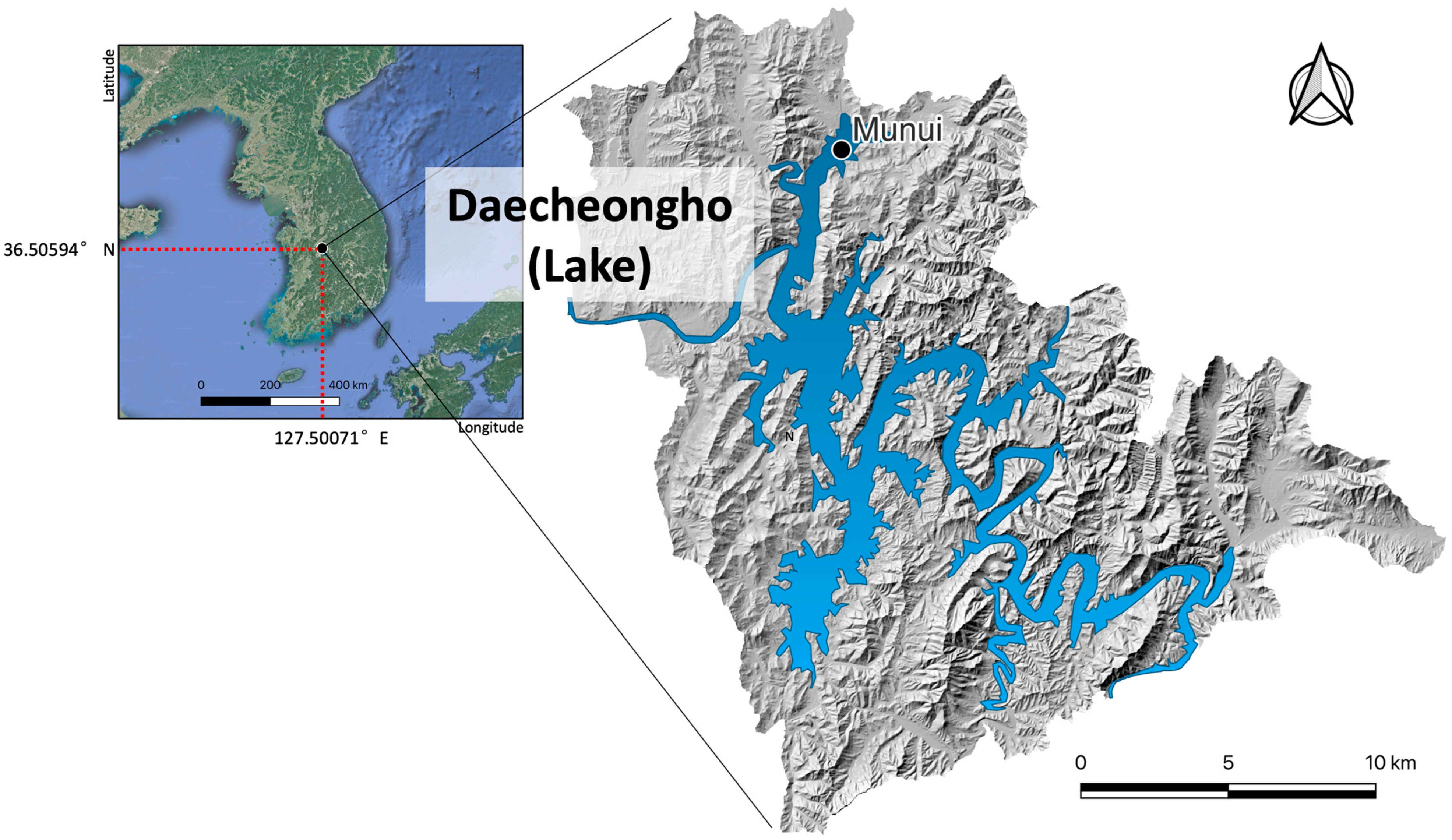
2.1. Study Site

Daecheong Lake is an artificial lake that is elongated along the north–south axis. It has a watershed area of 4184 km2, lake area of 72.8 km2, and lake volume of 1.5 billion m3. The study area was set up in Munui (latitude: 36.505945°; longitude: 127.500714°; average water depth: 17.4 ± 2.2 m; inter-annual variability in water depth: 11.3–22.1 m), which is located in an inlet area that is representative of the watershed environment and water quality in Daecheong Lake. The water quality and plankton community were surveyed twice per month (at the beginning of the month and after a fortnight) from March 2017 to November 2019, excluding the winter months (Figure 1).

2.2. Water Sampling and Measurement of Abiotic Factors

The water temperature was directly measured at the survey site using a sensor (YSI-6600, YSI, Yellow Springs, OH, USA). A water sample was collected, transported to the laboratory, and used for the measurement of total nitrogen (TN), total phosphorus (TP), and chlorophyll-a concentration (Chl-a). TN and TP were measured using a continuous flow analyzer (FUTURA 3, AMS Alliance, FREPILLON, France), and the Chl-a concentration was measured using a standard method for testing water quality (http://qaqc.nier.go.kr/qaqcnew/main.do, accessed on 15 August 2022).

2.3. Plankton Sampling

To sample the phytoplankton at the study site, 500 mL of raw water was collected in a sterile PE bottle and fixed immediately with Lugol’s solution (final concentration, 5%). In the laboratory, the collected sample was subjected to sedimentation for 24 h. The supernatant was discarded, and the concentrated sample (final volume, 20 mL) was mixed well. A subsample was extracted and placed in a Sedgewick Rafter chamber, and the genera of zooplankton were counted and identified under an optical microscope (Axioserver, Zeiss, Oberkochen, Germany; 40–100× magnification). The zooplankton were sampled onsite by vertically towing a plankton net (mesh size: 60 μm; diameter: 30 cm; length: 60 cm) through the water body at the study site. The sample was fixed in 4% neutral buffered formalin immediately after harvesting. The species and genera of zooplankton in the sample were identified under a dissecting microscope (SZ61, Olympus, Tokyo, Japan) and an optical microscope (Axio Imager M1, Zeiss) at 40–100× magnification. To identify zooplankton species, the methods reported by Patterson and Hedley were used for protozoa [40], while those reported by Flössner and Jeong et al. were used for rotifers and crustaceans [41,42]. Furthermore, copepods were identified using the methods reported by Chang [43]. Zooplankton abundance was estimated as individuals per liter (ind/L) based on the number of individuals counted per unit volume of raw water filtered (calculated based on the diameter and towing distance of the plankton net).

2.4. Analyzed Factors

2.4.1. Rotifer Groups

The variability in zooplankton community composition was estimated using rotifer groups, which are the dominant zooplankton group in Daecheong Lake. The rotifers observed during the survey period were classified into three groups based on their patterns of occurrence (abundance and frequency): (1) HAF: high abundance and frequency group; (2) MAF: medium abundance and frequency group; and (3) LAF: low abundance and frequency group. This helped minimize the underestimation of inter-species differences among zooplankton species with similar patterns of occurrence (e.g., species that occur throughout the year or those that occur temporarily for a short period of time).

2.4.2. Environmental Factors

To analyze the variability in rotifer community composition, we selected relevant abiotic environmental factors that can potentially affect rotifer community composition and identified relevant biotic factors based on known predator–prey interactions and inter-species competition [44,45,46,47]. The abiotic environmental factors included water temperature, TN, TP, and Chl-a concentration. Chl-a concentration represents the biomass value of total phytoplankton, while TN and TP represent nutrient concentration in lake ecosystems and act as limiting factors for phytoplankton growth [47,48]. Moreover, water temperature acts as the ultimate factor that determines the seasonality within the water body [49].
The biotic factors included the abundance data of copepods (excluding nauplii), cladocerans, nauplii, and various phytoplankton taxa (protozoa, green algae, blue-green algae, and diatoms) (Table 1).

2.5. Statistical Analysis

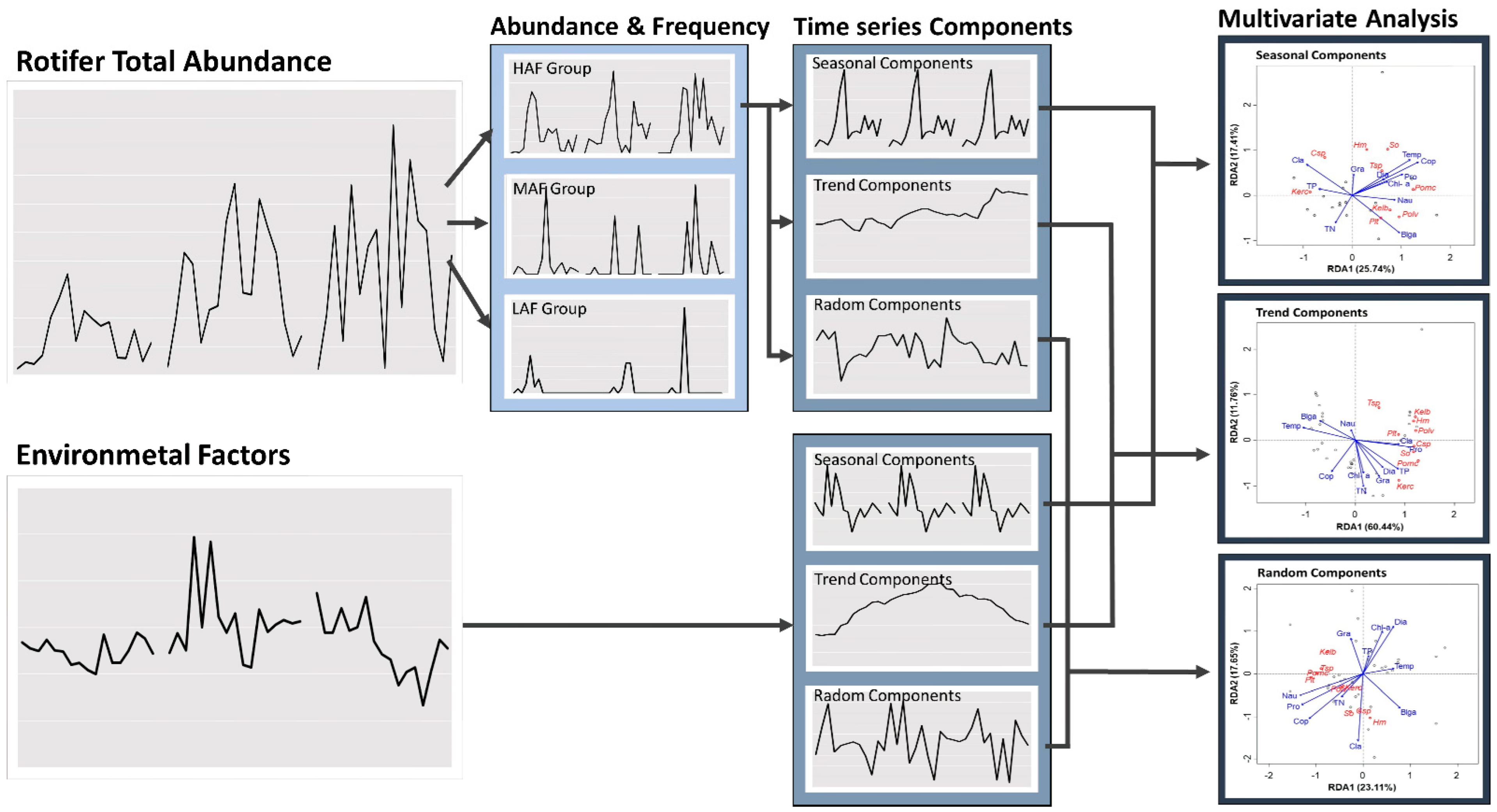
2.5.1. Decomposition Procedure

The Shapiro–Wilk test was conducted to confirm whether the data regarding rotifer abundance and environmental factors were normally distributed for data analysis. The results indicated that the data were normally distributed (p < 0.05). Using the classical decomposition method based on time series data, we classified the variability in the abundance of individual rotifer groups and in the associated environmental factors into seasonal and non-seasonal variability (further subdivided into inter-annual and intra-annual variability). The time series were decomposed into seasonal, trend, and random components using the additive decomposition model. The trend component was estimated using a centered moving average and was categorized as non-seasonal inter-annual variability. The seasonal component—obtained by averaging the values that remained after the trend component had been extracted—was categorized as seasonal variability. The random component was obtained by subtracting the trend and seasonal components from the rotifer abundance data and was categorized as non-seasonal intra-annual variability [50]. The decomposition method was performed using the “stats” package in R statistical software [51]. In addition, we used Pearson correlation coefficient analysis to assess the correlation between the abundance of each zooplankton group and time series components.

2.5.2. Multivariate Analysis Based on Decomposed Components

To evaluate the abundance patterns of rotifer species depending on changes in environmental factors, we performed redundancy analysis (RDA) for each of the aforementioned decomposed components using the “vegan” package in R. RDA, rather than canonical correlation analysis (CCA), was judged to be an appropriate method for data analysis based on the results of detrended correspondence analysis (DCA) using rotifer abundance and environmental factor data (gradient length < 4.0) [52,53]. All decomposed components of the three rotifer groups’ abundance (HAF, MAF, and LAF group) and environmental factors were analyzed. The decomposed components of each rotifer group were set as response variables for their respective analysis, and those of environmental factors were set as explanatory variables (Figure 2).

3. Results

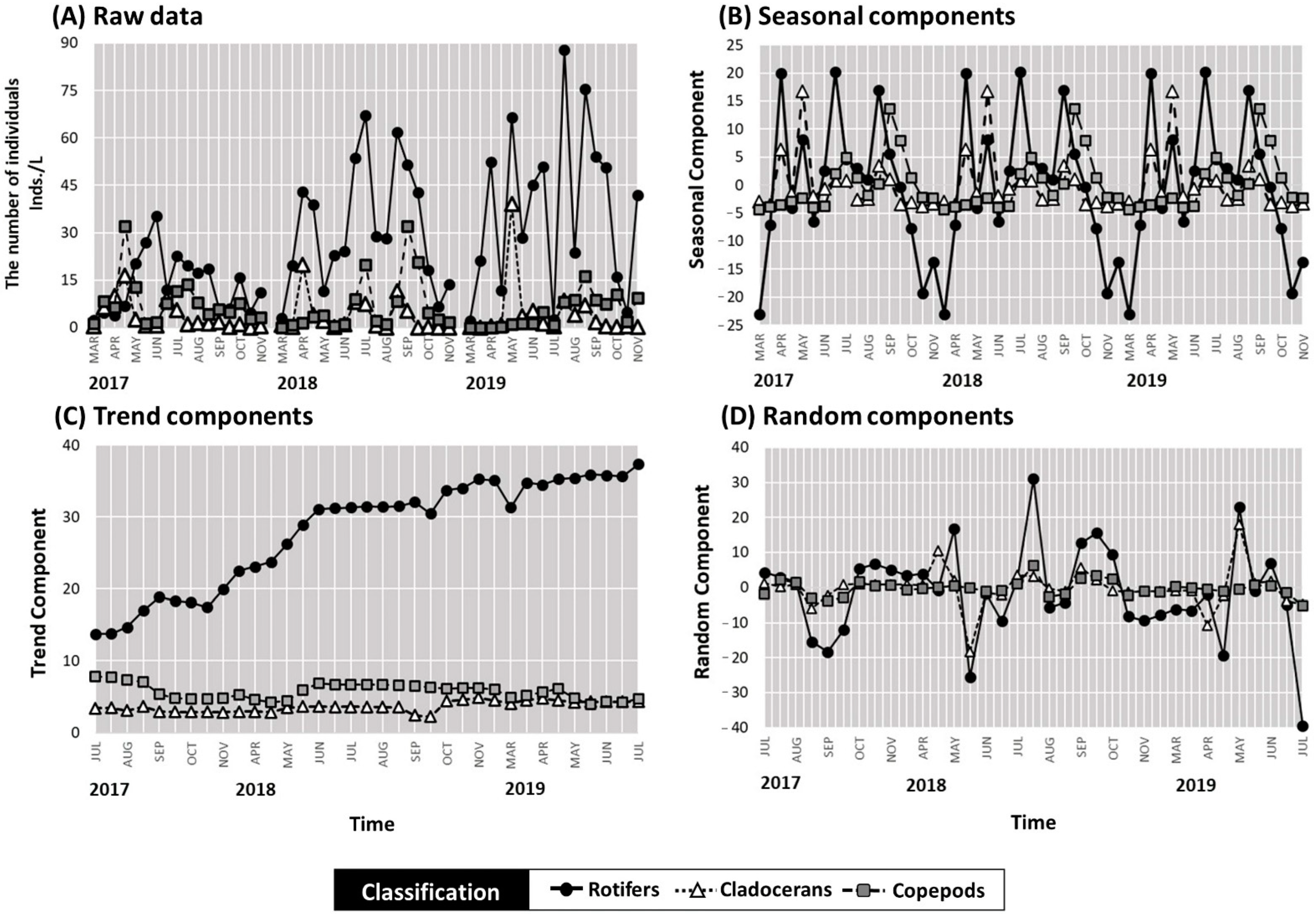
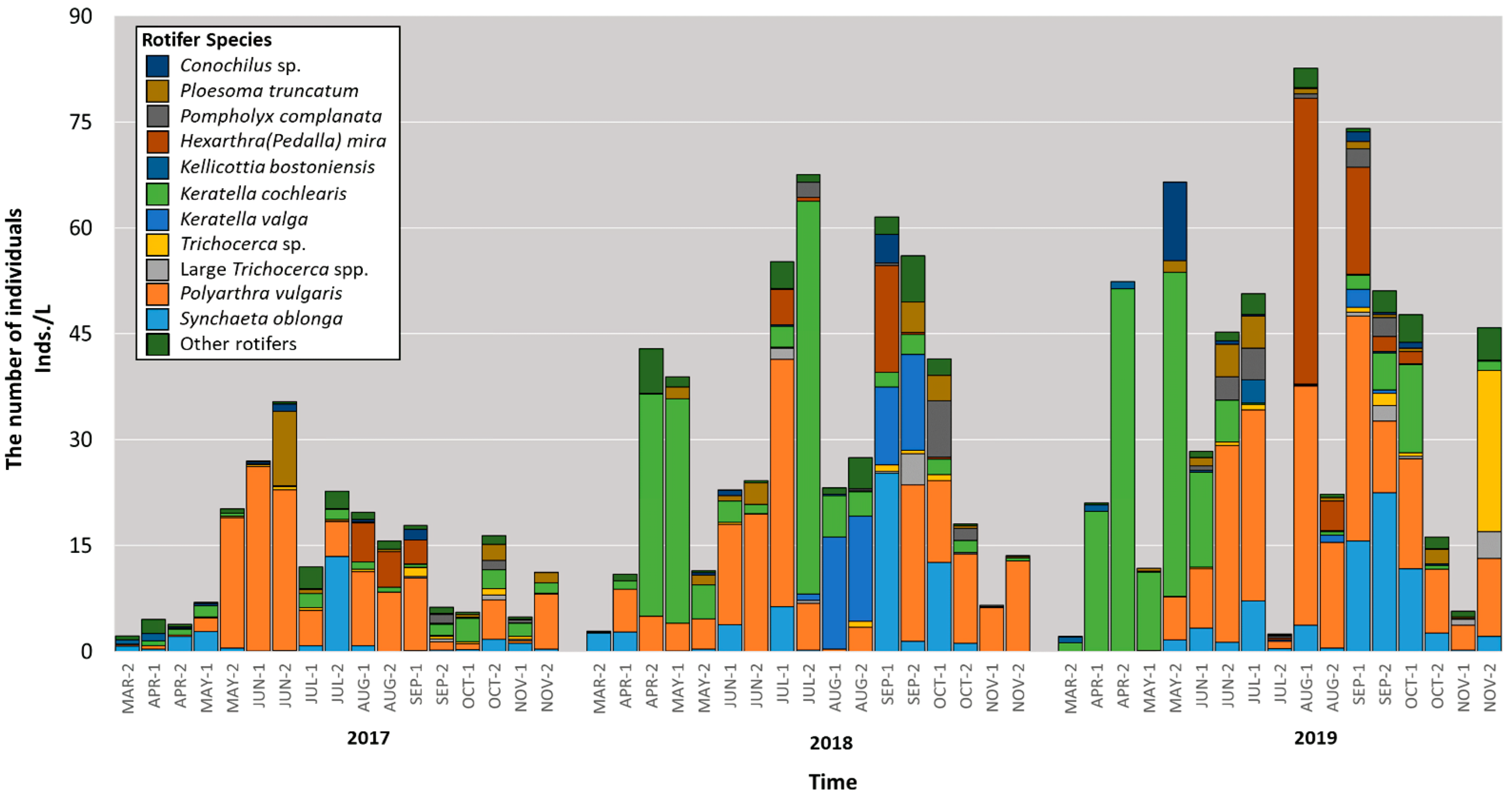
3.1. Variability in the Abundance of Zooplankton Groups and Results of the Time Series Analysis

The zooplankton groups recorded during the observation period (2017–2019) included 35 rotifer species and 9cladocerans. However, due to the difficulties in copepod identification, cyclopoids were only classified into adults (cyclopoid) and nauplii. Rotifers were the dominant taxa, accounting for 72.7% of the zooplankton population. Patterns of abundance varied between the zooplankton taxa (Figure 3A). Among rotifers, population peaks—that is, a rapid increase in the number of individuals within 1–2 months, followed by a rapid decrease within 1 month—were observed in the spring, summer, and autumn throughout the observation period. The time period of these peaks differed across the years (Figure 3A), as did the seasonally dominant species (Figure 4). There was an overall increase in the average abundance of rotifers in Daecheong Lake. Cladocerans did not occur in high numbers, except during 2–3 months of rapid population expansion. However, no cladocerans were observed in October and November. The populations of all cladoceran taxa peaked in April/May and in July/August, showing regular patterns of abundance (unlike copepods and rotifers; Figure 3A). Copepods (cyclopoids) were rarely observed, except during a low population peak each year (especially in July). However, the period of this population peak varied across the years (Figure 4).
The three components extracted from the time series of each zooplankton group were analyzed to elucidate the overall patterns of change throughout the observation period (Figure 5, Figure 6 and Figure 7). The seasonal components of rotifers and cladocerans showed similar patterns that coincided with the respective population peaks and patterns of variability in seasonal abundance (Figure 3B). Consequently, the seasonal components of rotifers and cladocerans were fairly highly correlated (r = 0.58). In contrast, the seasonal components of copepods showed no correlations with those of rotifers and cladocerans (Figure 3B). The trend component of rotifers showed a gradual and constant increase, reflecting the continuous increase in their average annual abundance (Figure 3C). However, the trend components of copepods and cladocerans showed no clear patterns, reflecting the lack of patterns in their respective abundance throughout the observation period. Similar to the seasonal components, the random components of rotifers and cladocerans also showed similar patterns. Most of the population peaks of rotifers coincided with those of cladocerans (Figure 3D), resulting in a fairly high correlation (r = 0.63). Moreover, the random components of copepods showed similar patterns to those of rotifers (Figure 3D). There was no marked variability in the random components of copepods; nevertheless, the recurrent population peaks of copepods throughout the observation period were similar to those of rotifers, resulting in a high correlation (r = 0.77) in random components. Thus, the findings related to random components deviated considerably from those related to seasonal components, as there was no correlation in seasonal components between rotifers and copepods.

3.2. Abundance-Based Classification of Rotifers

The 35 rotifer species recorded during the observation period were classified into three groups based on their abundance and frequency: (1) 9 species were classified into the HAF (high abundance and frequency) group (Polyarthra vulgaris, Keratella cochlearis, Hexarthra mira, Synchaeta oblonga, Pompholyx complanata, Ploesoma truncatum, Trichocerca sp., Conochilus sp., and Kellicottia bostoniensis), (2) 11 species were classified into the MAF (middle abundance and frequency) group (Filinia terminalis, large Trichocerca spp. (including elongata and cylindrica), Brachionus angularis, Filinia longiseta, Polyarthra euryptera, Kellicottia longispina, Brachionus quadridentatus, Lecane flexilis, Euchlanis dilatata, Monostyla closterocerca, and Asplanchna sp.), and (3) 13 species were classified into the LAF (low abundance and frequency) group (Keratella quadrata, Mytilina sp., Brachionus rubens, Brachionus calyciflorus, Monostyla sp., Asplanchna sieboldi, Brachionus sp., Brachionus forficula, Trichotria tetractis, Monostyla bulla, Lecane sp., Lecane luna, and Notholca labis) (Table 2).
Of the 35 rotifer species, Keratella valga and Ascomorpha ecaudis could not be classified into any of the groups because of their inconsistent abundance and frequency rankings. To evaluate whether the abundance patterns of these species were similar to those of any other rotifers in the three groups, we performed 1:1 correlation analysis with the three decomposed components of the other rotifer species. Keratella valga belonged to the HAF group in terms of abundance and the MAF group in terms of frequency. However, 1:1 correlation analysis revealed a high correlation (r = 0.78) with the seasonal component of Euchlanis dilatata (MAF), a very high correlation (r = 0.97) with the trend component of Brachionus quadridentatus (MAF), and a high correlation (r = 0.75) with the random component of Brachionus quadridentatus (MAF). Therefore, Keratella valga showed patterns similar to those of rotifers in the MAF group. Ascomorpha ecaudis belonged to the MAF group in terms of abundance and the HAF group in terms of frequency. The 1:1 correlation analysis revealed a high correlation (r = 0.71) with Asplanchna sp. (MAF) in the seasonal component, a high correlation (r = 0.84) with Brachionus rubens (LAF) in the trend component, and a fairly high correlation (r = 0.61) with Synchaeta oblonga (HAF) in the random component. Thus, Ascomorpha ecaudis showed high correlations with rotifers in all three groups, exhibiting abundance/frequency patterns different from those of all other rotifer species.

3.3. RDA of Rotifer Groups Based on Undecomposed Population Data

RDA revealed that the abundance and frequency of rotifers in the HAF group were related to water temperature, cladoceran abundance, and protozoan abundance. However, the associations were not statistically significant due to the low explanatory power (24.64%) of the first and second RDA axes (Figure 5A). The abundance and frequency of rotifers in the MAF and LAF groups were also partially associated with environmental factors (as shown in the RDA plot), but the explanatory power of the first and second RDA axes was very low (Figure 5B,C).

3.4. RDA of Rotifer Groups Based on the Seasonal Component

When the seasonal component was used for RDA, the first and second RDA axes explained the relationships between rotifer occurrence patterns and environmental factors to a greater extent than the RDA axes obtained using undecomposed population data. Each group of the rotifers was found to interact differently with environmental factors. In the HAF group, the two RDA axes explained 43.15% of the variance, and all rotifer species were significantly correlated on both axes (RDA species score > 0.5; Figure 6A). Moreover, rotifer species in the HAF group showed positive correlations with copepod abundance and water temperature. In the MAF group, the two RDA axes explained 47.31% of the variance. Rotifers in this group showed correlations with green algae, water temperature, nauplius abundance, and blue-green algae (in decreasing order; Figure 6B). In the LAF group, the two RDA axes explained 37.53% of the variance, and the explanatory power was lower than those in HAF and MAF (Figure 6C). Rotifer species in the LAF group were positively correlated with green algae, copepod abundance, water temperature, TN, nauplius abundance, diatoms, and Chl-a (in decreasing order). Overall, the analysis of seasonal components revealed that water temperature was significantly correlated with rotifers in all groups.

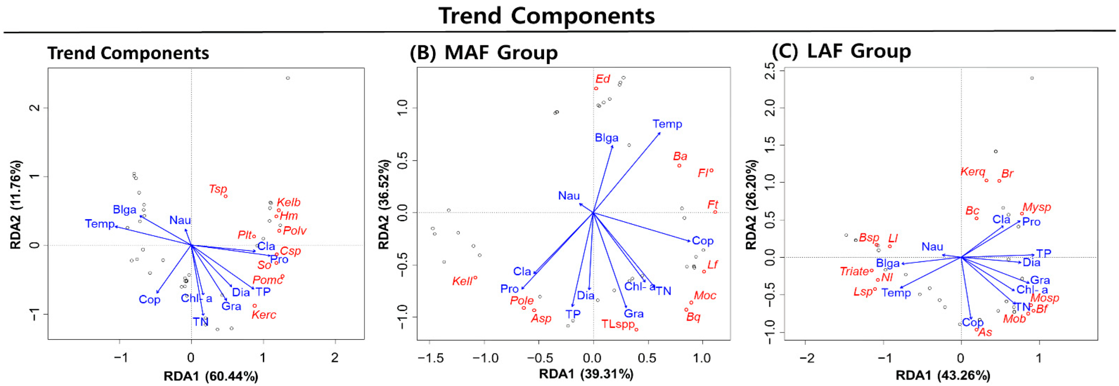
3.5. RDA of Rotifer Groups Based on the Trend Component

In all three groups, RDA based on the trend component resulted in first and second axes with approximately twice the explanatory power of those obtained from the analysis of the other two components (HAF: 72.2%; MAF: 75.83%; LAF: 69.46%; Figure 7). In addition, all rotifer species in the respective groups were significantly correlated with all environmental factors (except nauplius abundance). Rotifers in the HAF and MAF groups showed the highest correlations with protozoan abundance, whereas those in the LAF group showed the highest correlations with TP.

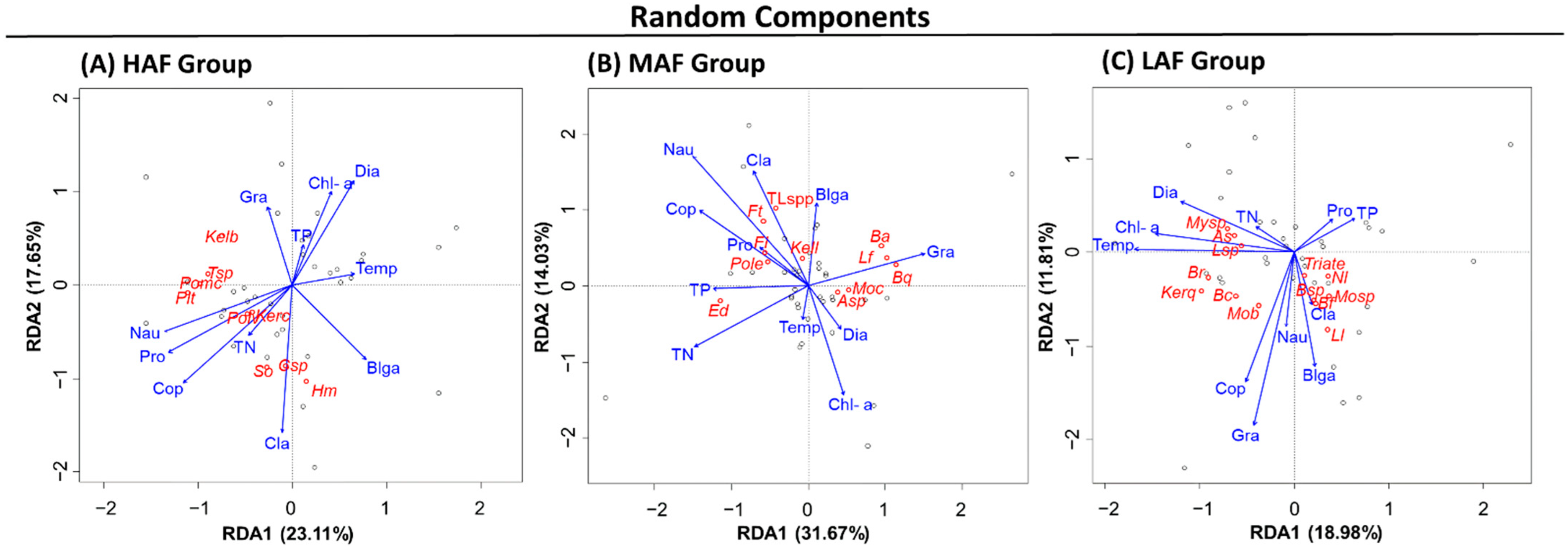
3.6. RDA of Rotifer Groups Based on the Random Component

Following RDA based on the random component, the first and second RDA axes explained 40.76%, 45.7%, and 30.79% of the variance in the HAF, MAF, and LAF groups, respectively. Thus, these results had higher explanatory power than those obtained from analyzing the undecomposed population data and lower explanatory power than those obtained from analyzing the other decomposed components (Figure 8). The explanatory power of the two RDA axes was lowest in the LAF group (Figure 8C). Rotifers in the HAF group were positively correlated with nauplii, protozoans, copepods, cladocerans, and diatoms (in decreasing order; Figure 8A). However, species-specific analysis could not be performed for two species (Polyarthra vulgaris and Keratella cochlearis) due to their low levels of interaction with environmental factors. Because these were high-frequency species, their abundance patterns may have been better explained by the seasonal and trend components. Rotifers in the MAF group were associated with nauplius abundance, TN, copepod abundance, green algae, and Chl-a (in decreasing order; Figure 8B), whereas those in the LAF group were associated with water temperature, diatoms, Chl-a, green algae, and copepods (in decreasing order; Figure 8C). Overall, the RDA of the random component revealed that none of the rotifer groups were associated with TP and blue-green algae, and all of them interacted with copepods. Notably, the three rotifer groups interacted differently with water quality (the environmental factor most closely associated with rotifer species composition).

4. Discussion

Long-term data (collected at regular intervals) on zooplankton community structure and related environmental factors can be used to assess changes in lake ecosystems and aquatic communities and to identify the causes of variability [1]. However, even data collected over several years can contain evidence of various fluctuations in population and community data, such as recurrent episodes of seasonal variations in populations and temporary fluctuations in species abundance. These patterns can often cause confusion when interpreting trends. Here, we evaluated how major environmental factors affect the zooplankton community in a lake. To this end, we categorized non-seasonal and seasonal variations in populations based on a time series analysis of changes in environmental factors and the abundance patterns of individual rotifer species. To facilitate this approach, rotifer species were classified into three groups based on their abundance and frequency patterns.
Compared with the RDA of undecomposed population data, the RDA of decomposed components had more explanatory power and better explained the relationships between rotifer occurrence and environmental factors. The multivariate analysis of population data (undecomposed raw data) had very low explanatory power (average: 17.39%). In contrast, RDA of the seasonal, trend, and random components explained 42.66%, 72.50%, and 39.08%, respectively, of the associations between rotifer occurrence patterns and environmental factors. This demonstrated that analyses based on decomposed components can provide better insights into these relationships than analyses based on undecomposed data. This improvement was particularly marked in the RDA results of rotifer species in the LAF group. Species in this group are difficult to study because of their seasonal occurrence. However, the analyses based on individual decomposed components yielded discernible results regarding the species abundance patterns and revealed concrete relationships between the occurrence patterns and environmental factors.
Although rotifers were more abundant than other taxa in the inlet area at Munui, only 9 of the 35 rotifer species showed high abundance and frequency overall (HAF). Several studies have investigated zooplankton species that are commonly found in freshwater ecosystems (such as Polyarthra vulgaris and Keratella cochlearis) and assessed their relationships with environmental factors (such as eutrophication and seasonal changes) [1,54]. However, there is limited scope for obtaining data on temporarily occurring species [55,56]. In this study, the RDA results based on undecomposed population data revealed positive relationships between rotifer species in the LAF group and environmental factors (such as water temperature and green algae). However, the results had very low explanatory power (10.49%), which makes it difficult to accurately identify any significant relationships. In contrast, the RDA results based on individual decomposed components revealed that seasonal variability was most closely associated with green algae, trend variability (non-seasonal inter-annual variability) with TP, and short-term intra-annual variability with water temperature. These environmental factors dominate the feeding environment, eutrophication, and seasonality in water bodies and are known to affect zooplankton community structure [57,58,59]. Classifying population variability into seasonal, non-seasonal inter-annual, and non-seasonal intra-annual variability allows us to extract the environmental factors associated with each type of variability. Therefore, this is considered to be an effective approach for elucidating the mechanisms underlying population-level changes in a given water body. In time series analysis, non-seasonal intra-annual variability is typically discarded as random noise and generally excluded from the analysis [30]. However, we included non-seasonal intra-annual variability in the zooplankton community in our analysis, which allowed us to examine the relationships between zooplankton species and environmental factors in more detail.
Multivariate analyses based on the seasonal component revealed that the abundance of rotifer species in all three groups was significantly associated with water temperature. Water temperature is generally considered to reflect seasonality in various environmental factors and aquatic communities [59]. By analyzing these data based solely on seasonal variability (that is, by separating seasonal vs. non-seasonal variability), it should still be possible to identify populations with cyclic seasonality vs. no seasonality based on their respective relationships with water temperature. Multivariate analyses based on the trend component revealed that the rotifer species in all three groups were positively correlated with all environmental factors (except nauplius abundance). This is inconsistent with the findings of a previous study that reported a close association between the total biomasses of rotifers and nauplii in various habitats [60]. Although nauplius abundance may be closely associated with the rotifer population, the association between these group has limited explanatory power for a direct relationship between nauplius abundance and individual rotifer species [61], as shown in this study. Follow-up studies are needed to investigate the relationships between the abundance patterns of individual species. To analyze the relationship between nauplii and rotifers using the methodology proposed in this study, more comprehensive data on rotifer abundance and frequency are required. Multivariate analyses based on random components revealed that rotifer abundance in all three groups was positively correlated with copepod abundance. This result is unexpected because copepod abundance is typically used as an indicator of predation pressure. It is possible that the favorable factors for both rotifer and copepod growth might have weakened the effect of predation [62,63].
In this study, we performed multivariate analysis by decomposing the population data of zooplankton and data related to various environmental factors into three decomposed components. We tested whether analyses based on individual decomposed components can better explain variations in the population structure of rotifer species with different patterns of temporal change. In lentic ecosystem, various environmental factors are intertwined and shape the species composition through species-specific interactions. However, the ways by which they affect species composition, particularly the time, period, and persistence of their impacts, are different. The water temperature and precipitation acting as ultimate factors increase or decrease significantly with periodicity, which gives strong seasonality to other related environmental factors within a year. At the same time, the temperature often continues to increase in a larger time scale due to global warming. On the other hand, unpredictable events such as the inflow of chemical pollutants including nutrients input in the lake can affect the community structure within a relatively short time period. In our analyses, by decomposing the environmental factors, we were able to extract different driving forces affecting the zooplankton community in different ways.
However, we have identified some aspects of the study that require further validation. Although multivariate analyses based on decomposed components showed clearer results than previously used analytical methods, further analyses using more comprehensive data are required to test the ecological significance of this approach. The species were categorized based on their patterns of variability in abundance, which introduces an inherent risk of bias. For example, when estimating the trend component, the moving average method was used for data smoothing by averaging the values adjacent to each time point. This invariably resulted in high correlations between the smoothed data. The statistical significance and ecological implications of such biased results will have to be tested further. Likewise, the results of multivariate analysis using this approach will have to be tested further to determine whether the enhanced explanatory power can properly explain the relationships between species occurrence patterns and environmental factors [64]. Another limitation of this study is that the classical time series analysis used in this study extracts values from the trend and random components. Therefore, it cannot be used to derive data points for the front and rear time points throughout the observation period [65], which reduces the plausibility of a direct comparison between the resulting data and original (undecomposed) population data. Additional analyses using the time series model may help elucidate the complex relationships between different decomposed components [66,67] and address the statistical limitations of this study. Finally, the three-year observation period in this study may be rather short, and the data may not be adequate for accurate interpretation based on time series analysis. Therefore, further research based on continuous and long-term monitoring is required to determine the correlations between the environmental factors and aquatic populations in the lake.

Author Contributions

Conceptualization, G.-H.H. and K.-H.C.; methodology, G.-H.H. and K.-H.C.; validation, K.-H.C. and H.-G.J.; formal analysis, G.-H.H.; data curation, S.H. and H.-G.J.; writing—original draft preparation, G.-H.H. and K.-H.C.; writing—review, K.-H.C., H.-G.J., H.-J.O. and Y.C.; writing—editing, K.-H.C., H.-J.O. and H.-G.J.; visualization, G.-H.H. and H.-J.O.; supervision, K.-H.C., H.-J.O., Y.C. and H.-G.J.; project administration, K.-H.C. and H.-G.J.; funding acquisition, K.-H.C. and H.-G.J. All authors have read and agreed to the published version of the manuscript.

Funding

This work was supported by the NIER R&D Project (grant number NIER 2022-01-01-075) of the National Institute of Environmental Research, funded by the Ministry of Environment (MOE) of the Republic of Korea.

Data Availability Statement

The datasets generated and/or analyzed during the study are available from the corresponding author on reasonable request.

Conflicts of Interest

The authors declare no conflict of interest.

References

  1. Gilbert, J.J. Suppression of rotifer populations by Daphnia: A review of the evidence, the mechanisms, and the effects on zooplankton community structure. Limnol. Oceanogr. 1988, 33, 1286–1303. [Google Scholar] [CrossRef]
  2. Pace, M.L.; Findlay, S.E.G.; Lints, D. Zooplankton in advective environments: The Hudson River community and a comparative analysis. Can. J. Fish. Aquat. Sci. 1992, 49, 1060–1069. [Google Scholar] [CrossRef]
  3. Gannon, J.E.; Stemberger, R.S. Zooplankton (especially crustaceans and rotifers) as indicators of water quality. Trans. Am. Microsc. Soc. 1978, 97, 16–35. [Google Scholar] [CrossRef]
  4. Lampert, W.; Fleckner, W.; Rai, H.; Taylor, B.E. Phytoplankton control by grazing zooplankton: A study on the spring clear-water phase. Limnol. Oceanogr. 1986, 31, 478–490. [Google Scholar] [CrossRef]
  5. Shurin, J.B. Interactive effects of predation and dispersal on zooplankton communities. Ecology 2001, 82, 3404–3416. [Google Scholar]
  6. Fischer, J.; Visbeck, M. Seasonal variation of the daily zooplankton migration in the Greenland Sea. Deep Sea Res. I 1993, 40, 1547–1557. [Google Scholar] [CrossRef]
  7. Jose, R.; Sanalkumar, M.G. Seasonal variations in the zooplankton diversity of River Achencovil. Int. J. Sci. Res. Publ. 2012, 2, 1–5. [Google Scholar]
  8. Buckley, L.J.; Durbin, E.G. Seasonal and inter-annual trends in the zooplankton prey and growth rate of Atlantic cod (Gadus morhua) and haddock (Melanogrammus aeglefinus) larvae on Georges Bank. Deep Sea Res. II 2006, 53, 2758–2770. [Google Scholar] [CrossRef]
  9. Allan, J.D. Life history patterns in zooplankton. Am. Nat. 1976, 110, 165–180. [Google Scholar] [CrossRef]
  10. Vargas, A.L.; Santangelo, J.M.; Bozelli, R.L. Recovery from drought: Viability and hatching patterns of hydrated and desiccated zooplankton resting eggs. Int. Rev. Hydrobiol. 2019, 104, 26–33. [Google Scholar] [CrossRef] [Green Version]
  11. Fernando, C.H. The freshwater zooplankton of Sri Lanka, with a discussion of tropical freshwater zooplankton composition. Int. Rev. Gesamten. Hydrobiol. Hydrogr. 1980, 65, 85–125. [Google Scholar] [CrossRef] [Green Version]
  12. Shurin, J.B. Dispersal limitation, invasion resistance, and the structure of pond zooplankton communities. Ecology 2000, 81, 3074–3086. [Google Scholar]
  13. Mackas, D.L.; Greve, W.; Edwards, M.; Chiba, S.; Tadokoro, K.; Eloire, D.; Mazzocchi, M.G.; Batten, S.; Richardson, A.J.; Johnson, C.; et al. Changing zooplankton seasonality in a changing ocean: Comparing time series of zooplankton phenology. Prog. Oceanogr. 2012, 97–100, 31–62. [Google Scholar] [CrossRef]
  14. Nogueira, M.G. Zooplankton composition, dominance and abundance as indicators of environmental compartmentalization in Jurumirim Reservoir (Paranapanema River), São Paulo, Brazil. Hydrobiologia 2001, 455, 1–18. [Google Scholar] [CrossRef]
  15. Kosobokova, K.N.; Hopcroft, R.R.; Hirche, H.-J. Patterns of zooplankton diversity through the depths of the Arctic’s central basins. Mar. Biodivers. 2011, 41, 29–50. [Google Scholar] [CrossRef]
  16. Lindeque, P.K.; Parry, H.E.; Harmer, R.A.; Somerfield, P.J.; Atkinson, A. Next generation sequencing reveals the hidden diversity of zooplankton assemblages. PLoS ONE 2013, 8, e81327. [Google Scholar] [CrossRef]
  17. Vincent, K.; Mwebaza-Ndawula, L.; Makanga, B.; Nachuha, S. Variations in zooplankton community structure and water quality conditions in three habitat types in northern Lake Victoria. Lakes Reserv. Res. Manag. 2012, 17, 83–95. [Google Scholar] [CrossRef]
  18. Roman, M.R.; Dam, H.G.; Gauzens, A.L.; Urban-Rich, J.; Foley, D.G.; Dickey, T.D. Zooplankton variability on the equator at 140 W during the JGOFS EqPac study. Deep Sea Res. II 1995, 42, 673–693. [Google Scholar] [CrossRef]
  19. Clark, R.A.; Frid, C.L.J.; Batten, S. A critical comparison of two long-term zooplankton time series from the central-west North Sea. J. Plankton. Res. 2001, 23, 27–39. [Google Scholar] [CrossRef] [Green Version]
  20. Colebrook, J.M. Continuous plankton records: Relationships between species of phytoplankton and zooplankton in the seasonal cycle. Mar. Biol. 1984, 83, 313–323. [Google Scholar] [CrossRef]
  21. Tavernini, S. Seasonal and inter-annual zooplankton dynamics in temporary pools with different hydroperiods. Limnologica 2008, 38, 63–75. [Google Scholar] [CrossRef] [Green Version]
  22. Araujo, H.M.P.; Nascimento-Vieira, D.A.; Neumann-Leitão, S.; Schwamborn, R.; Lucas, A.P.; Alves, J.P. Zooplankton community dynamics in relation to the seasonal cycle and nutrient inputs in an urban tropical estuary in Brazil. Braz. J. Biol. 2008, 68, 751–762. [Google Scholar] [CrossRef] [PubMed] [Green Version]
  23. Heinle, D.R. Temperature and zooplankton. Chesap. Sci. 1969, 10, 186–209. [Google Scholar] [CrossRef]
  24. Pepin, P.; Colbourne, E.; Maillet, G. Seasonal patterns in zooplankton community structure on the Newfoundland and Labrador Shelf. Prog. Oceanogr. 2011, 91, 273–285. [Google Scholar] [CrossRef]
  25. David, V.; Sautour, B.; Chardy, P.; Leconte, M. Long-term changes of the zooplankton variability in a turbid environment: The Gironde estuary (France). Estuar. Coast. Shelf Sci. 2005, 64, 171–184. [Google Scholar] [CrossRef]
  26. Richardson, A.J. In hot water: Zooplankton and climate change. ICES J. Mar. Sci. 2008, 65, 279–295. [Google Scholar] [CrossRef] [Green Version]
  27. Angeler, D.G.; Moreno, J.M. Zooplankton community resilience after press-type anthropogenic stress in temporary ponds. Ecol. Appl. 2007, 17, 1105–1115. [Google Scholar] [CrossRef]
  28. Greve, W.; Reiners, F.; Nast, J.; Hoffmann, S. Helgoland Roads meso-and macrozooplankton time-series 1974 to 2004: Lessons from 30 years of single spot, high frequency sampling at the only off-shore island of the North Sea. Helgol. Mar. Res. 2004, 58, 274–288. [Google Scholar] [CrossRef] [Green Version]
  29. Möllmann, C.; Müller-Karulis, B.; Kornilovs, G.; St John, M.A. Effects of climate and overfishing on zooplankton dynamics and ecosystem structure: Regime shifts, trophic cascade, and feedback loops in a simple ecosystem. ICES J. Mar. Sci. 2008, 65, 302–310. [Google Scholar] [CrossRef] [Green Version]
  30. Kostelich, E.J.; Schreiber, T. Noise reduction in chaotic time-series data: A survey of common methods. Phys. Rev. E 1993, 48, 1752–1763. [Google Scholar] [CrossRef]
  31. Mackas, D.L.; Beaugrand, G. Comparisons of zooplankton time series. J. Mar. Syst. 2010, 79, 286–304. [Google Scholar] [CrossRef]
  32. Yoshida, T.; Urabe, J.; Elser, J.J. Assessment of “top down” and ‘‘bottom-up’’ forces as determinants of rotifer distribution among lakes in Ontario, Canada. Ecol. Res. 2003, 18, 639–650. [Google Scholar] [CrossRef]
  33. Arndt, H. Rotifers as predators on components of microbial web (bacteria, heterotrophic flagellates, ciliates). Hydrobiologia 1993, 255, 231–246. [Google Scholar] [CrossRef]
  34. Gilbert, J.J. Further observations on developmental polymorphism and its evolution in the rotifer Brchionus calyciflorus. Freshw. Biolog. 1980, 10, 281–294. [Google Scholar] [CrossRef]
  35. Devetter, M. Influence of environmental factors on the rotifer assemblage in an artificial lake. Hydrobiologia 1998, 387–388, 171–178. [Google Scholar] [CrossRef]
  36. Liang, D.; Wang, Q.; Wei, N.; Tang, C.; Sun, X.; Yang, Y. Biological indicators of ecological quality in typical urban river-lake ecosystems: The planktonic rotifer community and its response to environmental factors. Ecol. Indic. 2020, 112, 106–127. [Google Scholar] [CrossRef]
  37. Chang, K.H.; Doi, H.; Imai, H.; Gunji, F.; Nakano, S.A. Longitudinal changes in zooplankton distribution below a reservoir outfall with reference to river planktivory. Limnology 2008, 9, 125–133. [Google Scholar] [CrossRef]
  38. Thouvenot, A.; Debroas, D.; Richardot, M.; Bertin Jugnia, L.; Dévaux, J. A study of changes between years in the structure of plankton community in a newly-flooded reservoir. Arch. Für Hydrobiol. 2000, 149, 131–152. [Google Scholar] [CrossRef]
  39. Lee, J.M.; Yoon, S.M.; Lee, J.J.; Park, J.G.; Lee, J.H.; Chang, C.Y. Zooplankton Fauna and the Interrelationship Among Cladoceran Populations and Microcystis aeruginosa (Cyanophyceae) during the Cyanobacterial Blooming Season at Daecheong Lake, South Korea. Korean J. Ecol. Environ. 2005, 38, 146–159. [Google Scholar]
  40. Patterson, D.J.; Hedley, S. Free-Living Freshwater Protozoa; CRC Press: London, UK, 1996. [Google Scholar]
  41. Flössner, D. Die Haplopoda und Cladocera (ohne Bosminidae) Mitteleuropas; Backhuys Publishers: Leiden, The Netherlands, 2000; p. 428. [Google Scholar]
  42. Jeong, H.G.; Kotov, A.A.; Lee, W. Checklist of the freshwater Cladocera (Crustacea: Branchiopoda) of South Korea. Proc. Biol. Soc. Wash. 2014, 127, 216–228. [Google Scholar] [CrossRef]
  43. Chang, C.Y. Illustrated Encyclopedia of Fauna & Flora of Korea: Inland Water Copepoda; Jeonghaeng-sa: Seoul, Republic of Korea, 2009; Volume 42. [Google Scholar]
  44. Williamson, C.E. Invertebrate predation on planktonic rotifers. Hydrobiologia 1983, 104, 385–396. [Google Scholar] [CrossRef]
  45. Gilbert, J.J. Competition between rotifers and Daphnia. Ecology 1985, 66, 1943–1950. [Google Scholar] [CrossRef]
  46. Bonecker, C.C.; Aoyagui, A.S.M. Relationships between rotifers, phytoplankton and bacterioplankton in the Corumbá reservoir, Goiás State, Brazil. In Rotifera X; Springer: Dordrecht, The Netherlands, 2005; pp. 415–421. [Google Scholar]
  47. Zhang, M.; Shi, X.; Yang, Z.; Yu, Y.; Shi, L.; Qin, B. Long-term dynamics and drivers of phytoplankton biomass in eutrophic Lake Taihu. Sci. Total Environ. 2018, 645, 876–886. [Google Scholar] [CrossRef]
  48. Pirasteh, S.; Mollaee, S.; Fatholahi, S.N.; Li, J. Estimation of phytoplankton chlorophyll-a concentrations in the Western Basin of Lake Erie using Sentinel-2 and Sentinel-3 data. Can. J. Remote Sens. 2020, 46, 585–602. [Google Scholar] [CrossRef]
  49. Zhu, C.; Zhang, J.; Nawaz, M.Z.; Mahboob, S.; Al-Ghanim, K.A.; Khan, I.A.; Lu, Z.; Chen, T. Seasonal succession and spatial distribution of bacterial community structure in a eutrophic freshwater Lake, Lake Taihu. Sci. Total Environ. 2019, 669, 29–40. [Google Scholar] [CrossRef]
  50. Kendall, M.; Stuart, A. The Advanced Theory of Statistics; Griffin: London, UK, 1983; Volume 3, pp. 410–414. [Google Scholar]
  51. R Core Team. R: A Language and Environment for Statistical Computing; R Foundation for Statistical Computing: Vienna, Austria, 2021; Available online: https://www.R-project.org/ (accessed on 15 August 2022).
  52. Hill, M.O.; Gauch, H.G. Detrended Correspondence Analysis: An Improved Ordination Technique. Vegetatio 1980, 42, 47–58. [Google Scholar] [CrossRef]
  53. Oksanen, J.; Simpson, G.; Blanchet, F.; Kindt, R.; Legendre, P.; Minchin, P.; O’Hara, R.B.; Solymos, P.; Stevens, M.H.H.; Szoecs, E.; et al. Vegan: Community Ecology Package. R Package Version 2013, 2, 321–326. Available online: https://CRAN.R-project.org/package=vegan (accessed on 15 August 2022).
  54. Zhao, C.; Liu, C.; Zhao, J.; Xia, J.; Yu, Q.; Eamus, D. Zooplankton in highly regulated rivers: Changing with water environment. Ecol. Eng. 2013, 58, 323–334. [Google Scholar] [CrossRef]
  55. Inaotombi, S.; Gupta, P.K.; Mahanta, P.C. Influence of abiotic factors on the spatio-temporal abundance of rotifers in a subtropical lake of western Himalaya. Water Air Soil Poll. 2016, 227, 1–15. [Google Scholar] [CrossRef]
  56. Nandini, S.; Sánchez-Zamora, C.; Sarma, S.S.S. Toxicity of cyanobacterial blooms from the reservoir Valle de Bravo (Mexico): A case study on the rotifer Brachionus calyciflorus. Sci. Total Environ. 2019, 688, 1348–1358. [Google Scholar] [CrossRef]
  57. Schlüter, M.; Groeneweg, J.; Soeder, C.J. Impact of rotifer grazing on population dynamics of green microalgae in high-rate ponds. Water Res. 1987, 21, 1293–1297. [Google Scholar] [CrossRef]
  58. Dodds, W.K.; Bouska, W.W.; Eitzmann, J.L.; Pilger, T.J.; Pitts, K.L.; Riley, A.J.; Schloesser, J.T.; Thornbrugh, D.J. Eutrophication of US freshwaters: Analysis of potential economic damages. Environ. Sci. Technol. 2009, 43, 12–19. [Google Scholar] [CrossRef] [Green Version]
  59. May, L. Rotifer occurrence in relation to water temperature in Loch Leven, Scotland. Hydrobiologia 1983, 104, 311–315. [Google Scholar] [CrossRef]
  60. Park, G.S.; Marshall, H.G. The trophic contributions of rotifers in tidal freshwater and estuarine habitats. Estuar. Coast. Shelf Sci. 2000, 51, 729–742. [Google Scholar] [CrossRef]
  61. Lehtovaara, A.; Arvola, L.; Keskitalo, J.; Olin, M.; Rask, M.; Salonen, K.; Sarvala, J.; Tulonen, T.; Vuorenmaa, J. Responses of zooplankton to long-term environmental changes in a small boreal lake. Boreal Environ. Res. 2014, 19, 97–111. [Google Scholar]
  62. Karabin, A. The pressure of pelagic predators of the genus Mesocyclops (Copepoda, Crustacea) on small zooplankton. Ekol. Pol. 1978, 26, 241–257. [Google Scholar]
  63. Stemberger, R.S.; Evans, M.S. Rotifer seasonal succession and copepod predation in Lake Michigan. J. Great Lakes Res. 1984, 10, 417–428. [Google Scholar] [CrossRef]
  64. Storch, H.V. Misuses of statistical analysis in climate research. In Analysis of Climate Variability; Springer: Berlin, Germany, 1999; pp. 11–26. [Google Scholar]
  65. Yule, G.U. Why do we sometimes get nonsense-correlations between time-series?—A study in sampling and the nature of time-series. J. R. Stat. Soc. 1926, 89, 1–63. [Google Scholar] [CrossRef]
  66. Findley, D.F.; Monsell, B.C.; Bell, W.R.; Otto, M.C.; Chen, B.C. New capabilities and methods of the X-12-ARIMA seasonal-adjustment program. J. Bus. Econ. Stat. 1998, 16, 127–152. [Google Scholar]
  67. Cleveland, R.B.; Cleveland, W.S.; McRae, J.E.; Terpenning, I. STL: A seasonal-trend decomposition. J. Off. Stat. 1990, 6, 3–73. [Google Scholar]
Figure 1. Survey site at Munui in an inlet area of Daecheongho (a lake in South Korea).
Water 14 04113 g001
Figure 2. Time series data to elucidate the relationship between the abundance patterns of rotifers and environmental factors.
Water 14 04113 g002
Figure 3. Inter-annual changes (2017–2019) in the number of zooplankton individuals by taxon (A) and patterns of change in the seasonal (B), trend (C), and random (D) components derived from the time series of rotifers, cladocerans, and copepods in Daecheong Lake.
Water 14 04113 g003
Figure 4. Inter-annual changes (2017–2019) in the number of rotifers by species in Daecheong Lake; top 11 species and others based on three-year patterns of abundance found in the pooled samples.
Water 14 04113 g004
Figure 5. Redundancy analysis of the undecomposed population data (raw data into time series components) of three rotifer groups and relevant environmental factors. (A) High abundance and frequency rotifers group, (B) Middle abundance and frequency rotifers group, (C) Low abundance and frequency rotifers group. Abbreviations: Temp, temperature; Cla, cladoceran; Cop, copepod; Nau, nauplii; Pro, protozoa; Blga, blue-green algae; Dia, diatom; Gra, green algae; Polv, Polyarthra vulgaris; Kerc, Keratella cochlearis; So, Synchaeta oblonga; Hm, Hexarthra mira; Plt, Ploesoma truncatum; Tsp, Trichocerca sp.; Pomc, Pompholyx complanata; Csp, Conochilus sp.; Kelb, Kellicottia bostoniensis; TLspp, Large Trichocerca spp. (T. elongata, T. cylindrica); Fl, Filinia longiseta; Moc, Monostyla closterocerca; Ft, Filinia terminalis; Ed, Euchlanis dilatate; Ba, Brachionus angularis; Pole, Polyarthra euryptera; Asp, Asplanchna sp.; Lf, Lecane flexilis; Kell, Kellicottia longispina; Bq, Brachionus quadridentatus; Kerq, Keratella quadrata; Mysp, Mytilina sp.; Bf, Brachionus forficula; As, Asplanchna sieboldin; Bsp, Brachionus sp.; Mob, Monostyla bulla; Br, Brachionus rubens; Bc, Brachionus calyciflorus; Lsp, Lecane sp.; Mosp, Monostyla sp.; Triate, Trichotria tetractys; Ll, Lecane luna; Nl, Notholca labis.
Water 14 04113 g005
Figure 6. Redundancy analysis of the seasonal component (derived from the time series of the abundance estimates of three rotifer groups) and environmental factors. (A) High abundance and frequency rotifers group, (B) Middle abundance and frequency rotifers group, (C) Low abundance and frequency rotifers group.
Water 14 04113 g006
Figure 7. Redundancy analysis of the trend components (derived from the time series of the abundance estimates of three rotifer groups) and environmental factors. (A) High abundance and frequency rotifers group, (B) Middle abundance and frequency rotifers group, (C) Low abundance and frequency rotifers group.
Water 14 04113 g007
Figure 8. Redundancy analysis of the random component (derived from the time series of the abundance estimates of three rotifer groups) and environmental factors. (A) High abundance and frequency rotifers group, (B) Middle abundance and frequency rotifers group, (C) Low abundance and frequency rotifers group.
Water 14 04113 g008
Table 1. Summary of 11 environmental factors that may influence the species composition of the rotifer community in Daecheong Lake.
Environment FactorValueUnitMinMaxAverageSDCV (%)
Water Quality FactorTemperature°C6.5327.719.366.2332.15
TNmg/L0.662.4731.370.3323.82
TPmg/L0.000.0520.020.0159.80
Chl-amg/m30.0039.113.806.66175.23
Biological FactorCladoceransind/L0.0039.113.806.66175.23
Copepodsind/L0.0012.822.893.01104.03
Naupliiind/L0.0026.473.515.08144.58
Protozoaind/L0.0053.615.6410.76190.78
Blue-green algaecells/mL0.00345,53812,409.8849,921.40402.27
Diatomcells/mL8.003472596.63743.86124.68
Green algaecells/mL4.001190223.53270.94121.21
Note: Abbreviations: Min, minimum; Max, maximum; SD, standard deviation; CV, coefficient of variation; ind, individuals; Chl-a, chlorophyll a; TN, total nitrogen; TP, total phosphorus.
Table 2. Summary of the community data (number of individuals, number of species ratio, and frequency) for rotifer species abundance and frequency 2017–2019 in Daecheong Lake.
Abundance RankRotifer SpeciesTotal Individuals (ind/L)Species Ratio (%)FrequencyRotifer Group
1Polyarthra vulgaris489.3335.12747HAF Group
2Keratella cochlearis342.3724.57748HAF Group
3Synchaeta oblonga155.0611.13140HAF Group
4Hexarthra (Pedalla) mira99.627.15117HAF Group
5Keratella valga60.624.35212*
6Ploesoma truncatum49.343.54232HAF Group
7Trichocerca sp.38.132.73729HAF Group
8Pompholyx complanata30.532.19219HAF Group
9Conochilus sp.24.171.73519HAF Group
10Kellicottia bostoniensis241.72319HAF Group
11Large Trichocerca spp. (elongata, cylindrica) 16.251.16717MAF Group
12Ascomorpha ecaudis12.690.91120*
13Filinia longiseta9.550.68612MAF Group
14Monostyla closterocerca9.450.6788MAF Group
15Filinia terminalis5.050.3635MAF Group
16Euchlanis dilatata4.590.32912MAF Group
17Brachionus angularis4.410.3175MAF Group
18Polyarthra euryptera3.730.2685MAF Group
19Asplanchna sp.3.50.25111MAF Group
20Lecane flexilis2.450.1765MAF Group
21Kellicottia longispina1.980.1423MAF Group
22Brachionus quadridentatus1.760.1263MAF Group
23Keratella quadrata0.940.0672LAF Group
24Mytilina sp.0.630.0452LAF Group
25Brachionus forficula0.50.0363LAF Group
26Asplanchna sieboldi0.390.0282LAF Group
27Brachionus sp.0.360.0262LAF Group
28Monostyla bulla0.30.0222LAF Group
29Brachionus rubens0.280.0201LAF Group
30Brachionus calyciflorus0.260.0191LAF Group
31Lecane sp.0.260.0193LAF Group
32Monostyla sp.0.260.0191LAF Group
33Trichotria tetractis0.160.0111LAF Group
34Lecane luna0.080.0061LAF Group
35Notholca labis0.040.0031LAF Group
Note: * Not included in the rotifer for the analysis.
Publisher’s Note: MDPI stays neutral with regard to jurisdictional claims in published maps and institutional affiliations.

