
Future Changes in Temperature and Precipitation over Northeastern Brazil by CMIP6 Model
by
 , , , and
Leydson G. Dantas
1,
Carlos A. C. dos Santos
1,*,
Celso A. G. Santos
2 ,
,
Eduardo S. P. R. Martins
3 and
Lincoln M. Alves
4 1
Academic Unity of Atmospheric Sciences, Federal University of Campina Grande, Campina Grande 58109-970, PB, Brazil
2
Department of Civil and Environmental Engineering, Federal University of Paraíba, João Pessoa 58051-900, PB, Brazil
3
Foundation Cearense for Meteorology and Water Resources, Fortaleza 60115-221, CE, Brazil
4
National Institute for Space Research, Earth System Science Center, São José dos Campos 12227-010, SP, Brazil
*
Author to whom correspondence should be addressed.
Water 2022, 14(24), 4118; https://doi.org/10.3390/w14244118
Submission received: 7 November 2022
/
Revised: 12 December 2022
/
Accepted: 13 December 2022
/
Published: 16 December 2022
(This article belongs to the Section Water and Climate Change)
Abstract
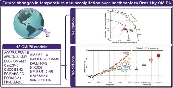
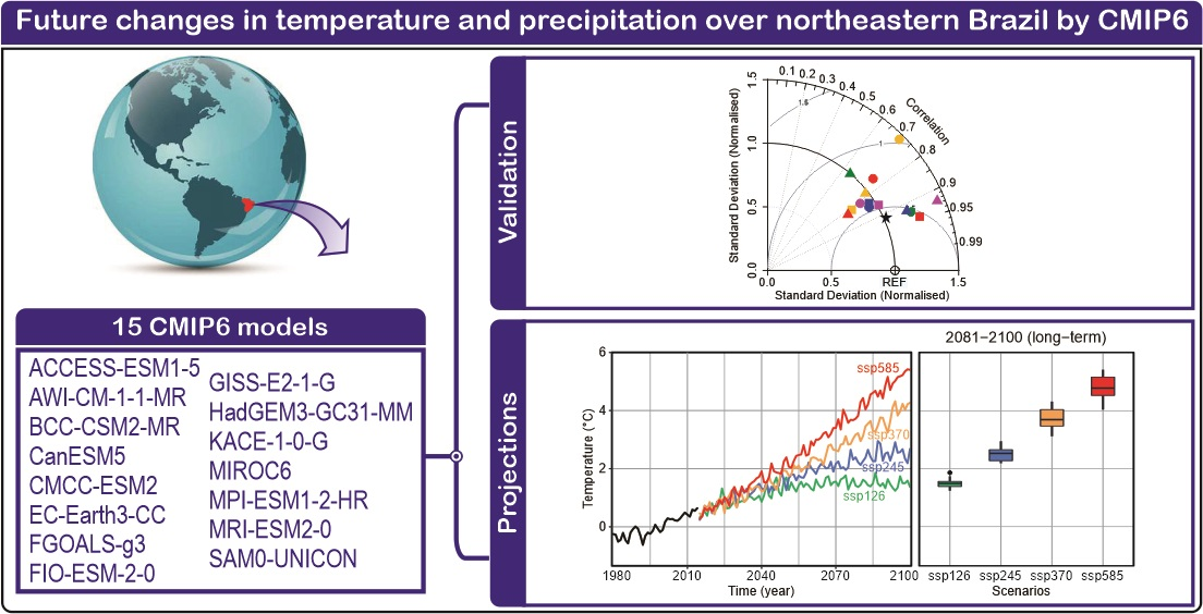
:Global warming is causing an intensification of extreme climate events with significant changes in frequency, duration, and intensity over many regions. Understanding the current and future influence of this warming in northeastern Brazil (NEB) is important due to the region’s greater vulnerability to natural disasters, as historical records show. In this paper, characteristics of climate change projections (precipitation and air temperature) over NEB are analyzed using 15 models of Coupled Model Intercomparison Project Phase 6 (CMIP6) under four Shared Socioeconomic Pathways (SSPs: SSP1-2.6, SSP2-4.5, SSP3-7.0, and SSP5-8.5) scenarios. By using the Taylor diagram, we observed that the HadGEM3-GC31-MM model simulates the seasonal behavior of climate variables more efficiently. Projections for NEB indicate an irreversible increase in average air temperature of at least 1 °C throughout the 21st century, with a reduction of up to 30% in annual rainfall, as present in scenarios of regional rivalry (SSP3-7.0) and high emissions (SSP5-8.5). This means that a higher concentration of greenhouse gases (GHG) will increase air temperature, evaporation, and evapotranspiration, reducing rainfall and increasing drought events. The results obtained in this work are essential for the elaboration of effective strategies for adapting to and mitigating climate change for the NEB.
1. Introduction
In a recent publication, Working Group I of the Sixth Assessment Report of the Intergovernmental Panel on Climate Change (IPCC) emphatically stated that human activities are irrefutably responsible for the abnormal warming of the atmosphere, continents, and oceans and, consequently, are responsible for climate change [1]. Without immediate actions to reduce emissions, the world will fail to comply with the Paris Agreement, which proposed stabilizing the temperature increase at 1.5 °C in the next decade [1]. The greater intensity and frequency of drought and flood events, caused by increased temperatures, is the focus of several global research projects associated with climate change issues, as these climate changes result in negative impacts on water security, notably, in arid and semiarid regions of the planet [2,3,4,5].
In NEB, three sub-regions with different rainfall regimes are identified: The East Coast has its maximum rainfall in May, the Interior has its maximum rainfall in December, and the North has its maximum rainfall in March [6,7,8]. The climate in these regions is highly influenced by the Sea Surface Temperatures (SSTs) of the Tropical Atlantic and Pacific Oceans [9,10]. The main atmospheric systems that influence the climate in NEB are the Intertropical Convergence Zone (ITCZ) [11,12], South Atlantic Convergence Zone (SACZ) [13], cold fronts [6], Upper Tropospheric Cyclonic Vortices (UTCVs) [14], and Easterly Wave Disturbances (EWD) [15], presented in the synoptic scale. Mesoscale Convective Complexes (MCCs) [16], instability lines, and sea–land breezes [17] are presented in the mesoscale. On the local scale, isolated storms, and the circulation of valley–mountain breezes [18] are observed.
The residents of the Brazilian semiarid region experience frequent periods of water scarcity [7,19,20] caused by the high natural climate variability of rainfall on both spatial and temporal scales [21,22,23]. Historically, the NEB has experienced several droughts, such as in 1877–1878, when human activities had little impact on the global climate [24]. From 1877 onwards, other major droughts occurred in 1900, 1915, 1919, 1932, 1942, 1951–1953, 1958, 1970, 1979–1983, 1987, 1990, 1992–1993, 1997–1998, 2002–2003, 2012–2018, and 2021 [3,7,20,25,26]. In addition, climate change, often in combination with other problems, such as lack of food and unemployment caused by drought, has resulted in population migration (mostly rural) to other regions of Brazil, [20]. Understanding the current and future characteristics of temperature, precipitation, storms, floods, and droughts is important for planning actions related to society, including prevention and mitigation measures.
In the recent literature on climate change in South America (SA), different regions of interest were studied [27,28,29], but none of them focused on the whole NEB, rather only on some representative areas [30,31,32]. Thus, there is a demand to apply analyses of climate projections to the entire area to gather the information that helps in the understanding of how climate change will possibly impact different portions of the region. This may provide helpful information on setting up a climate change adaptation and mitigation plan for the region, substantially reducing GHG emissions in the coming decades, and contributing to climate-resilient pathways for sustainable development [33].
The Global Climate Models (GCMs) are used to better understand the functioning of the climate system. In this way, it is possible to simulate the historical behavior of the variables as well as to elaborate climate projections on global and regional scales [33,34]. In a collective effort to standardize assessments of GCMs on this scale, researchers have been improving climate modeling with the advancement of science and computational capacity, thus producing different phases of the Coupled Model Intercomparison Project (CMIP). This has provided data on several GCMs for both past and future periods. CMIP-derived products are the basis for climate-change-related assessments [35] and have contributed in recent years to the analyses presented by the Intergovernmental Panel on Climate Change (IPCC) [31,36]. This makes it possible to observe the evolution and potential of models to simulate large-scale historical phenomena and, therefore, enables their use in studies associated with climate change [35,37,38,39,40].
These models foster climate science by helping researchers understand how the change in land cover, the use of fossil fuels, and the human-induced degradation of natural resources unbalance the climate system. In this study, the CMIP6 models, the most current version among the CMIPs, are applied. The scenarios analyzed different possibilities of evolution and development as well as considered the challenges of mitigating and adapting to climate change. This context could be achieved when the mitigation targets of Representative Concentration Pathways (RCPs) are combined with Shared Socioeconomic Pathways (SSPs) [41,42,43]. These models present improved spatial resolution of physical parameterization and better representations of the processes associated with the Earth system and its components [35,40], resulting in greater climate sensitivity in their products [44].
It has already been observed that the CMIP6 models capture the main characteristics of the variable precipitation over South America [29]. These suggest more intense and lasting droughts, with fewer days of rain during the historically rainy season, thus resulting in higher temperatures in the northeastern portion of SA [45]. However, in this analysis, the high climatic variability in NEB was not carefully considered, as the authors used an average representative of the entire area, together with other locations in Brazil, which could lead to errors in their analysis since the rainy season in NEB starts at different times in each subregion. Due to this characteristic, more specific analyses of the NEB climate are necessary.
In this context, it is necessary to carry out studies on climate variability and their projections from the point of view of the new emission scenarios presented in CMIP6 and to provide suitable products for decision-makers. To strengthen this knowledge, it is necessary to carry out focused research on changes in precipitation and air temperature, which may help identify possible changes in climate patterns. Thus, this work aims to analyze the performance of 15 GCMs derived from CMIP6 in simulating the general characteristics of the historical behavior of precipitation and air temperature near the surface over three areas of the NEB and, after validation, generate projections for these two variables corresponding to four climate projection scenarios until the end of the 21st century.
2. Materials and Methods
2.1. Study Area
The Northeastern Brazilian region (NEB), shown in Figure 1, is characterized by average annual precipitation of approximately 800 mm, which may seem high, but with evapotranspiration exceeding 2000 mm and shallow soils and a crystalline basement, adaptation to this condition is already a challenge at present [46].
2.2. CMIP6 Models
We used historical data and projections of monthly precipitation and air near-surface temperature from 15 GCMs included in the CMIP6 experiments [36] and available on the Earth System Grid Federation portal (https://esgf-node.llnl.gov/search/cmip6/, accessed on 27 October 2021). Information on these models is shown in Table 1, along with the ensemble member, country of origin, atmospheric model component, and atmospheric resolution. These were selected due to their efficiency in reproducing the general characteristics of the precipitation and temperature variables in recent international studies around the globe [29,47,48,49]. The ensemble members are divided into four indices that represent the global attributes specific to each model: “r” for realization, “i” for initialization, “p” for physics, and “f” for forcing. The ensemble names “r1i1p1f1” and “r1i1p1f3” suggest that the ensemble members present the same initial and physical conditions but with different forcings, where “f1” is forcing derived from atmospheric model intercomparison project (AMIP) one-moment aerosol (OMA) simulations, and “f3” is forcing derived from E2.2 OMA simulations (ozone field update).
Although the historical simulations of CMIP6 cover the period from 1850 to 2014, the interval from 1980 to 2014 was selected for validation, as it is the most recent historical period (not bias-corrected) and has been used in recent research, including studies by the IPCC [50,51,52]. Shared socio-economic pathways (SSPs) describe probable configurations of the climate system according to global economic development scenarios [53]. Therefore, four SSPs were selected to analyze greenhouse gas emissions scenarios in each model using different climate policies between 2015 and 2100.
The SSPs discussed are: SSP1-2.6, which targets the world with economic development, low use of fossil fuels, and, therefore, sustainability; SSP3-7.0, which addresses regional disputes over natural resources; SSP5-8.5, which analyzes fossil-fuel-based economic development; and SSP2-4.5, which is the common ground among all the other SSPs. They are all included in the CMIP6 to complement the RCP introduced in the Coupled Model Intercomparison Project Phase (CMIP5) [54,55]. The SSPs are labeled as SSPX-Y, where “X” varies from 1 to 5 and identifies five socioeconomic scenario groups. In contrast, “Y” varies from 1.9 to 8.5 and characterizes the approximate radiative forcing of the 21st century [35].
2.3. Observation Data
We used near-surface air temperature data as well as precipitation information on a monthly scale with 0.5° resolution from the Climatic Research Unit gridded Time Series (CRU-TS) v. 4.03 [56,57] from 1980 to 2014. This database was chosen because it contains the desirable variables for this analysis in a high-resolution global terrestrial surface grid. CRU TS data are available from the Center for Environmental Data Analysis (CEDA: https://data.ceda.ac.uk//badc/cru/data/cru_ts/, accessed on 25 October 2021) or on the CRU website (https://crudata.uea.ac.uk/cru/data/hrg/, accessed on 25 October 2021). The climatic variables were analyzed in three subregions of NEB, namely the East Coast, Interior, and North of the NEB, all highlighted in Figure 1. In addition to the well-defined seasonal cycle, the selection of these subregions is due to their relevance in climatic, hydrological, and social studies of the NEB [6,7,8].
2.4. Methods
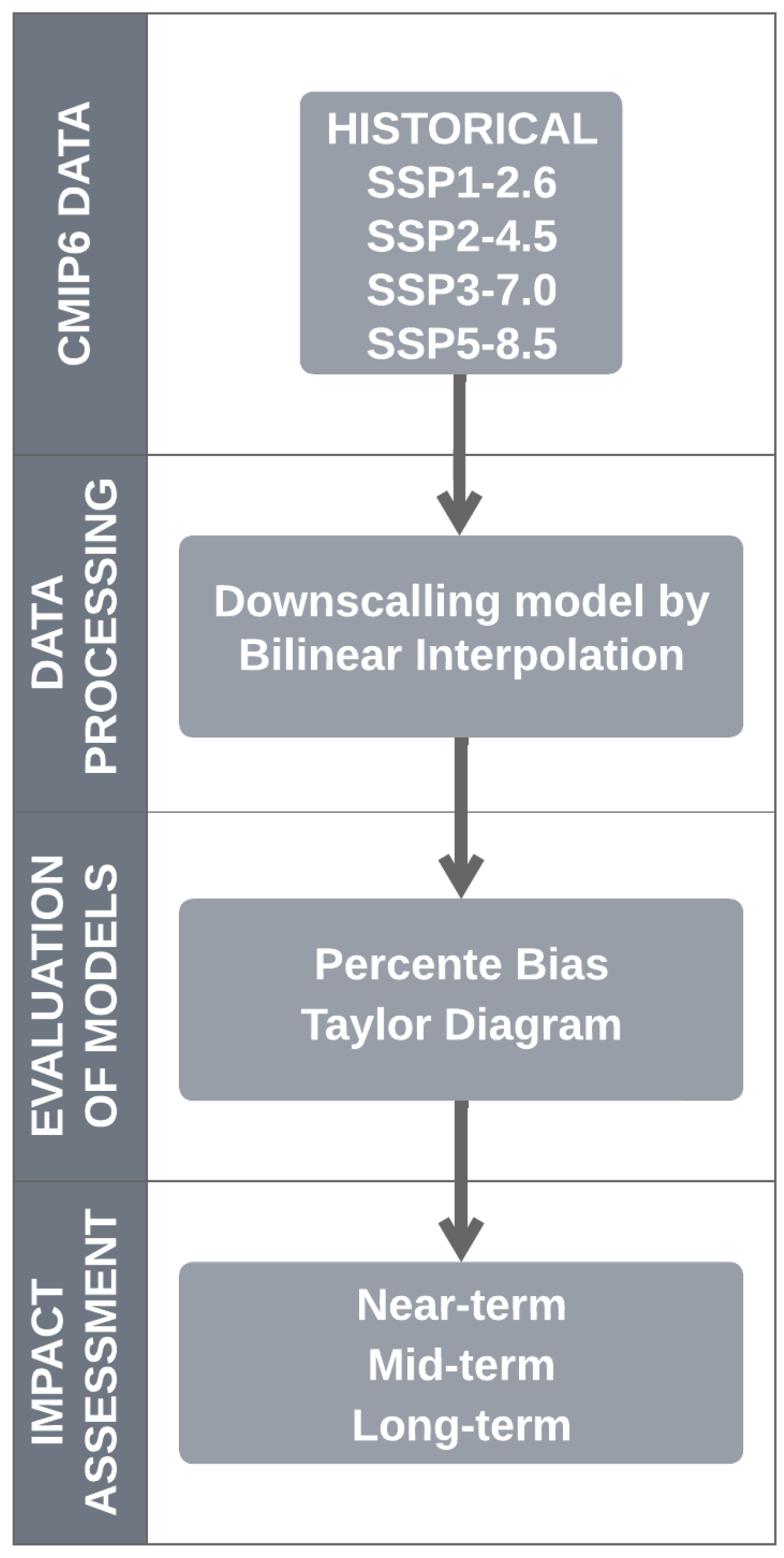
Since each GCM has its own spatial resolution, as shown in Table 1, each GCM output was spatially remapped by bilinear interpolation (statistical downscaling) to a typical grid of 1° × 1°. After these calculations, the simulations of each GCM could be verified for the historical period of reference and adjusted to the climatology of the same period in terms of percentage of bias and mean. The percent bias was used to qualitatively assess the simulation of the average behavior of monthly precipitation and air temperature near the surface by the 15 GCMs. This technique identifies the average tendency of the simulated values and, therefore, helps to understand the months in which there is underestimation and overestimation of the model in relation to the reference information for the current climate (1980–2014) for the elaboration of heat maps.
The Taylor diagram was applied to validate the CMIP6 used in this study, and ranking elaboration was used to quantify their spatial similarity with the reference data [36,58]. This technique graphically gives information about the performance of models when using various statistical criteria, such as root-mean-square error (RMSE), Pearson’s correlation coefficient (R), and standard deviation (SD) [59]. Assuming that R and normalized SD are close to 1 and the RMSE is 0, the model performs perfectly. On the basis of these metrics, the best models representing the seasonal precipitation and temperature cycles (all seasons) were chosen, and the climate change assessment was performed. As a result of this selection, 15 GCMs and the ensemble of the top five models were used to analyze climate change scenarios (SSPs) until the end of the 21st century. Therefore, the structure applied in this study consists of four steps, ranging from data acquisition to projections, as highlighted in Figure 2.
3. Results
3.1. Assessment of CMIP6 Simulations
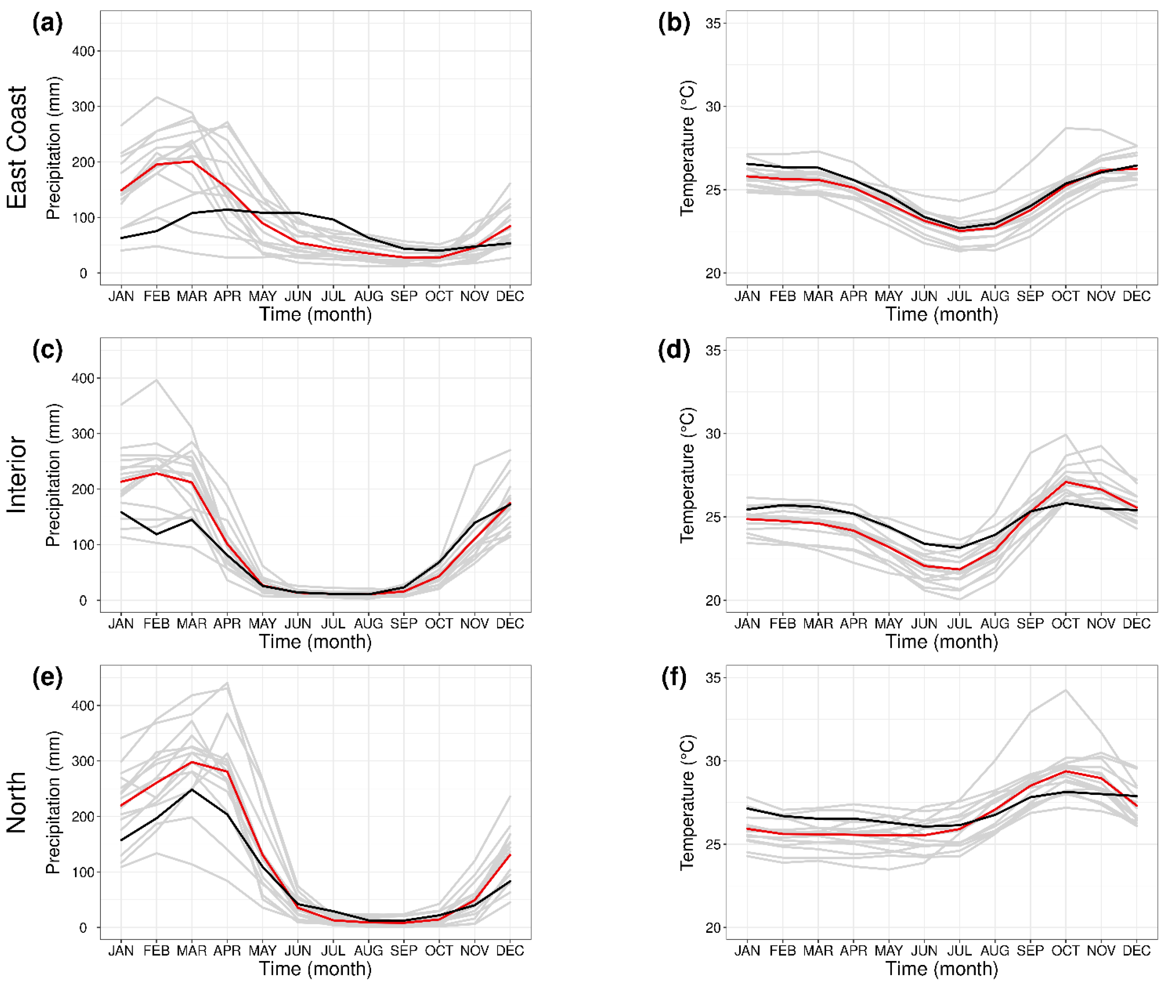
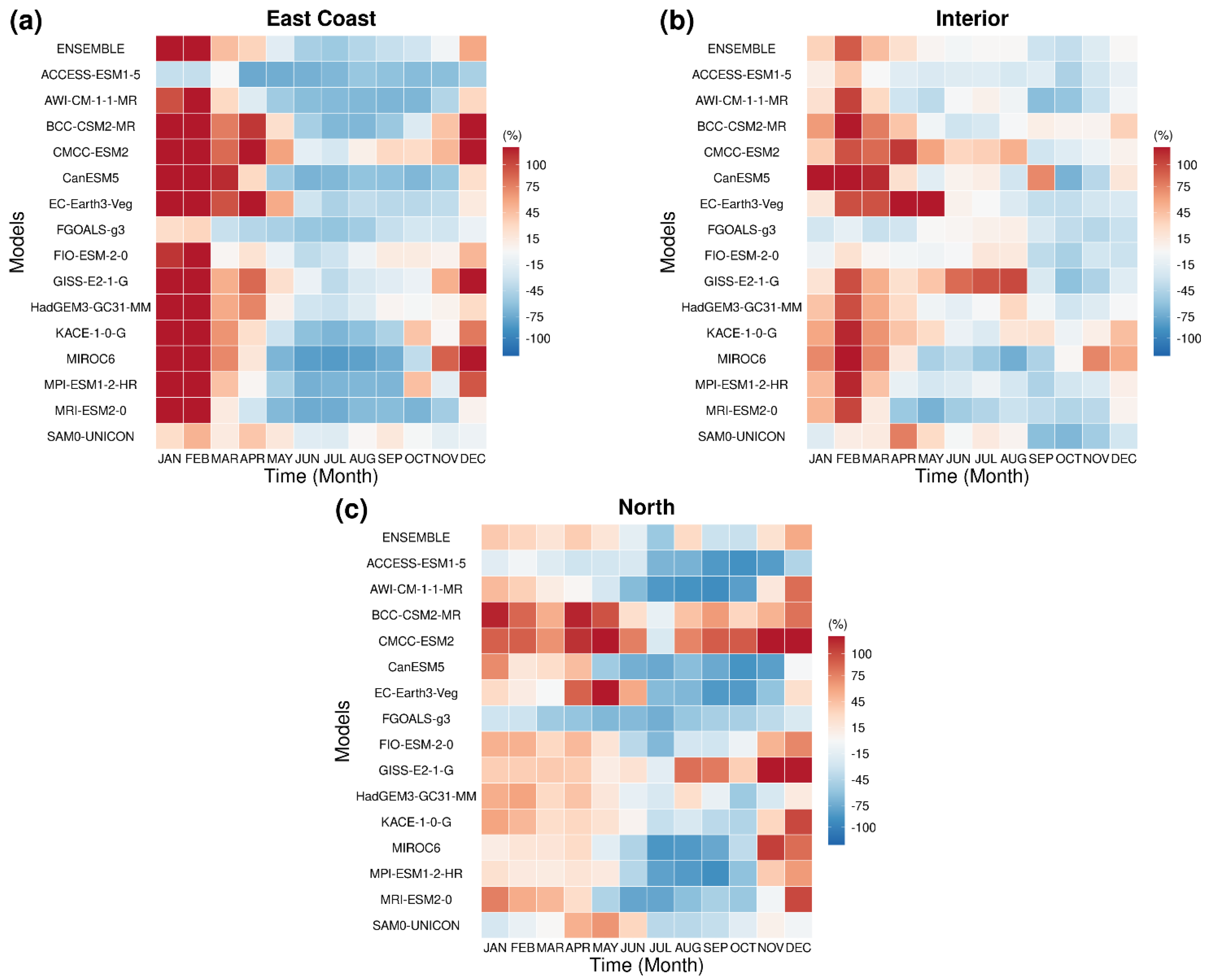
The capacity of the models to distinguish the wet and dry periods for the region is evident in Figure 3, where the monthly averages of precipitation, the temperature of the CMIP6 models, and the reference data are shown. The descriptive analysis (percent bias) of how the 15 CMIP6 models and the ensemble simulate the annual cycle of these variables over the study area is shown in Figure 4 and Figure 5, respectively. The study used a reference period from 1980 to 2014.
On the East Coast (Figure 4a), most models (12 of 15) overestimate rainfall during the austral summer, a period with rainfall volumes concentrated in the southernmost regions of this subregion. In addition, eight out of fifteen models strongly underestimate precipitation characteristics during the austral winter. The CanESM5, BCC-CSM2-MR, and MPI-ESM1-2-HR models have less ability to simulate the climatological variability of the region, due mainly to the overestimation of precipitation during the austral summer. However, some models stand out for reproducing a value close to that which was observed; they are FIO-ESM-2-0, FGOALS-g3, and SAM0-UNICON.
In the rainy season, 11 out of the 15 models indicate overestimated precipitation over the Interior of the NEB (Figure 4b). The CMCC-ESM2, CanESM5, EC-Earth3-Veg, and GISS-E2-1-G models overestimate the historical precipitation. The ACCESS-ESM1-5, FIO-ESM-2-0, SAM0-UNICON, and FGOALS-g3 models fit better due to their low bias in relation to the reference data. In addition, the ensemble product can reproduce the variability of the annual cycle.
Historical simulations, such as those from the ACCESS-ESM1-5, AWI-CM-1-1-MR, MIROC6, and MPI-ESM1-2-HR models, showed the ability to represent rainfall in the NEB. The models’ simulations continue to overestimate the average rainfall in the rainy season for the North subregion (Figure 4c), except for the FGOALS-g3 model, which significantly underestimates the precipitation during the rainy season. In this evaluation, 12 of the 15 models overestimated precipitation, with the CMCC-ESM2, BCC-CSM2-MR, and MRI-ESM2-0 models doing so the most, particularly for March and April.
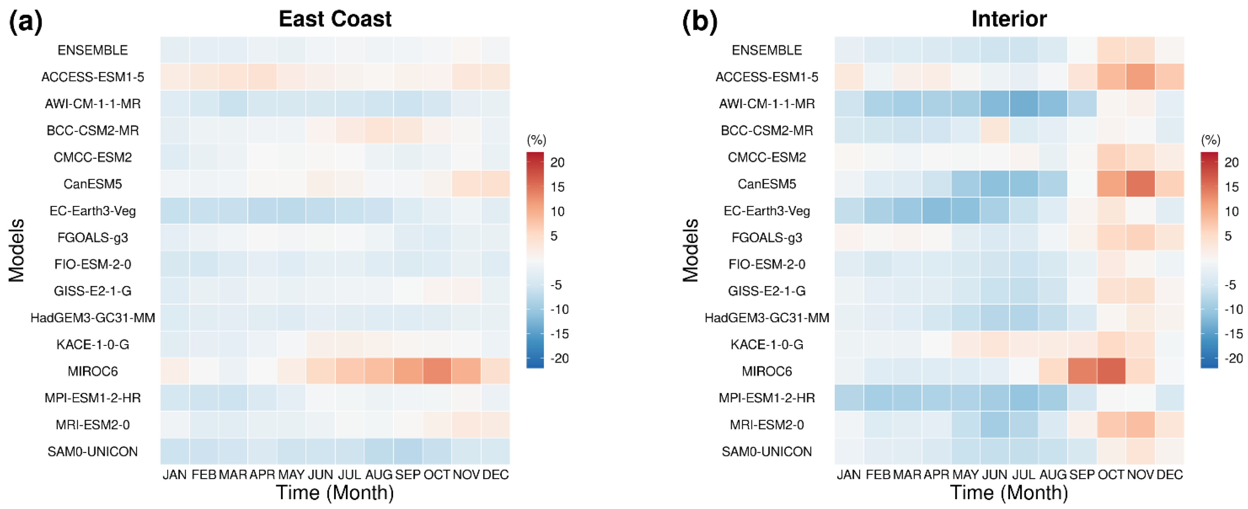
The simulation of the annual cycle of mean air temperature near the surface (CRU-TS4) is presented in Figure 3 and Figure 5. The pattern associated with underestimating mean surface temperature (3 of 15 models) during the austral winter is noted on the NEB East Coast (Figure 4a). The AWI-CM-1-1-MR, EC-Earth-Veg, and SAM0-UNICON models stand out for underestimating the temperature value, and the MIROC6 for overestimating it. However, in this subregion, the models can adjust to the characteristics of the reference data due to the low bias found. The best-performing models are the CMCC-ESM2, GISS-E2-1-G, KACE-1-0-G, and MRI-ESM2-0. The ensemble performed better than any other model by observing bias.
In the Interior (Figure 5b), most models indicate an underestimation of the temperature during the summer (3 of 15 models) and austral winter (6 of 15 models), and some of these models overestimate the temperature during the austral spring (7 of 15 models). The AWI-CM-1-1-MR, CanESM5, MPI-ESM1-2-HR, MRI-ESM2-0, and SAM0-UNICON have the highest temperature bias. On the other hand, models such as the CMCC-ESM2, KACE-1-0-G, ACCESS-ESM1-5, and FGOALS-g3 present a better fit to the reference values relative to the others. The ensemble tends to underestimate temperature behavior over months, but it reproduces the signal of the annual temperature cycle.
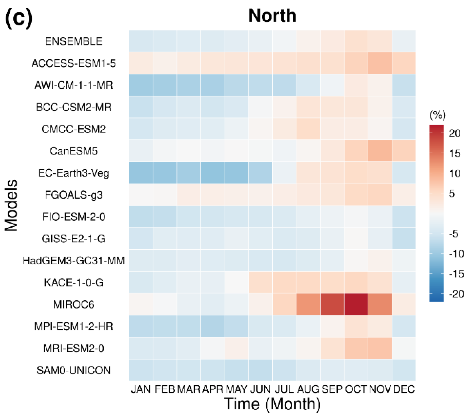
In the North subregion of NEB (Figure 5c), underestimation of temperature by the CMIP6 models (5 of 15) continues to be observed, with the difference occurring during the austral summer and the autumn. The high magnitude of temperatures during the austral spring is another notable feature (7 of 15 models). High absolute values of minimum and maximum magnitudes are observed in the AWI-CM-1-1-MR, EC-Earth3-Veg, FIO-ESM-2-0, MPI-ESM1-2-HR, and SAM0-UNICON models. The model with the best performance and, therefore, with the lowest bias value is the CMCC-ESM2. The ensemble showed the ability to simulate the temporal variability of the annual cycle of mean surface air temperature.
According to the temporal analyses elaborated for the temperature, the East Coast is the subregion where the CMIP6 models present the most remarkable ability to simulate the climatology of this temperature. However, in other areas, some CMIP6 models can simulate history. The underestimation of the values is observed more frequently during the austral winter, while the overestimation is more frequent in the austral spring. In recent studies, similar patterns have also been observed in South America [60,61]. Therefore, selecting the best models for ensemble formation is essential, as a poor selection of these can compromise its performance [62]. This indicates the necessity to apply statistical methodologies that focus on quantitative assessment and, thus, help select the best models to simulate historical conditions. Once the models are chosen, the ensemble is expected to provide more efficient climate projections due to the quality presented in simulating recent climate.
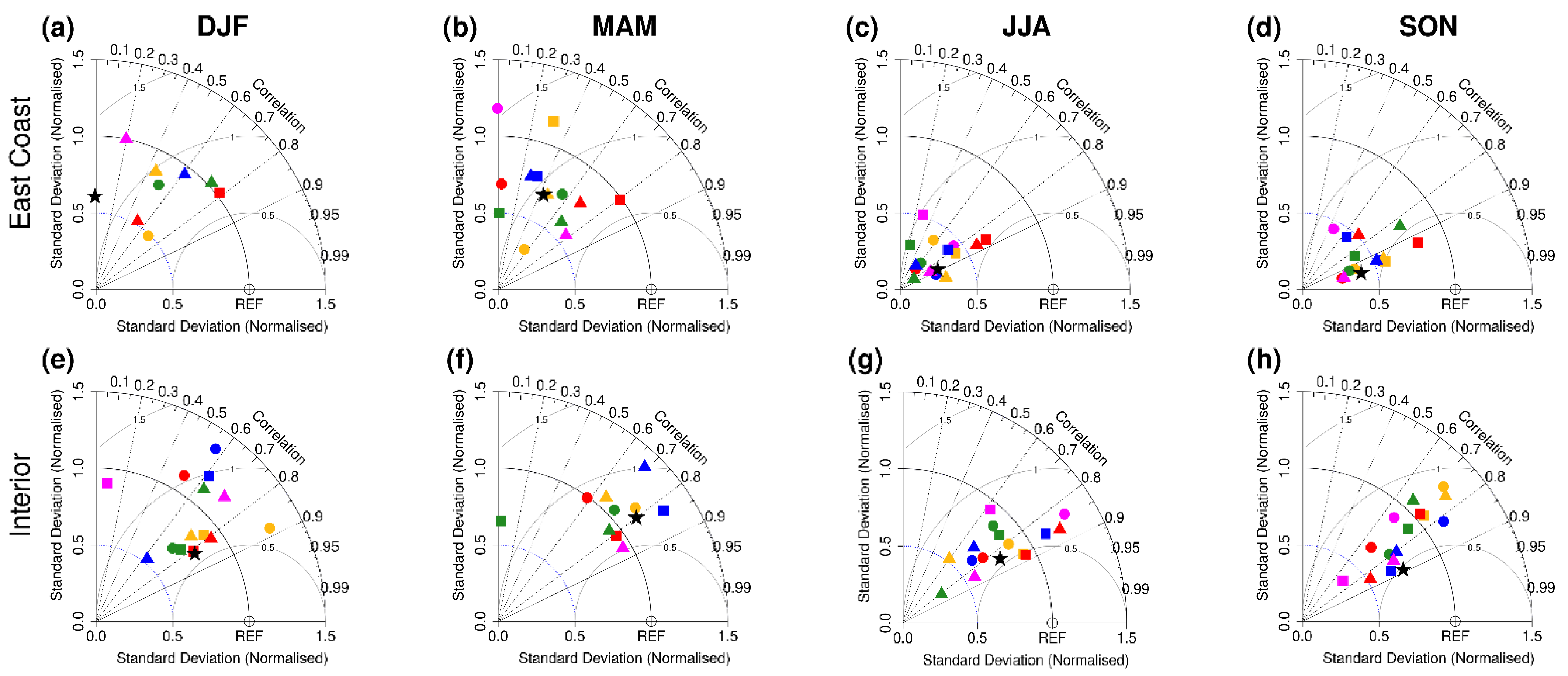
The Taylor diagram is frequently used to assess the efficiency of GCMs in simulating observed spatial patterns [63,64,65]. This diagram can graphically summarize how closely a set of models matches the observations [66] by providing RMSE, R, and SD. Therefore, the Taylor diagram distinguished the models with greater skill among the 15 CMIP models available in Table 1.
The seasonal comparison between the reference data and simulations by the CMIP6 models is carried out with the Taylor diagram to validate the variables precipitation and temperature, as shown in Figure 6 and Figure 7. The symbols correspond to the spatial simulation of each model studied and to the ensemble. Models identified with a correlation value greater than 0.6, a standard deviation between 1.00 ± 0.25, and an RMSE less than 1, are highlighted as the best performers [62].
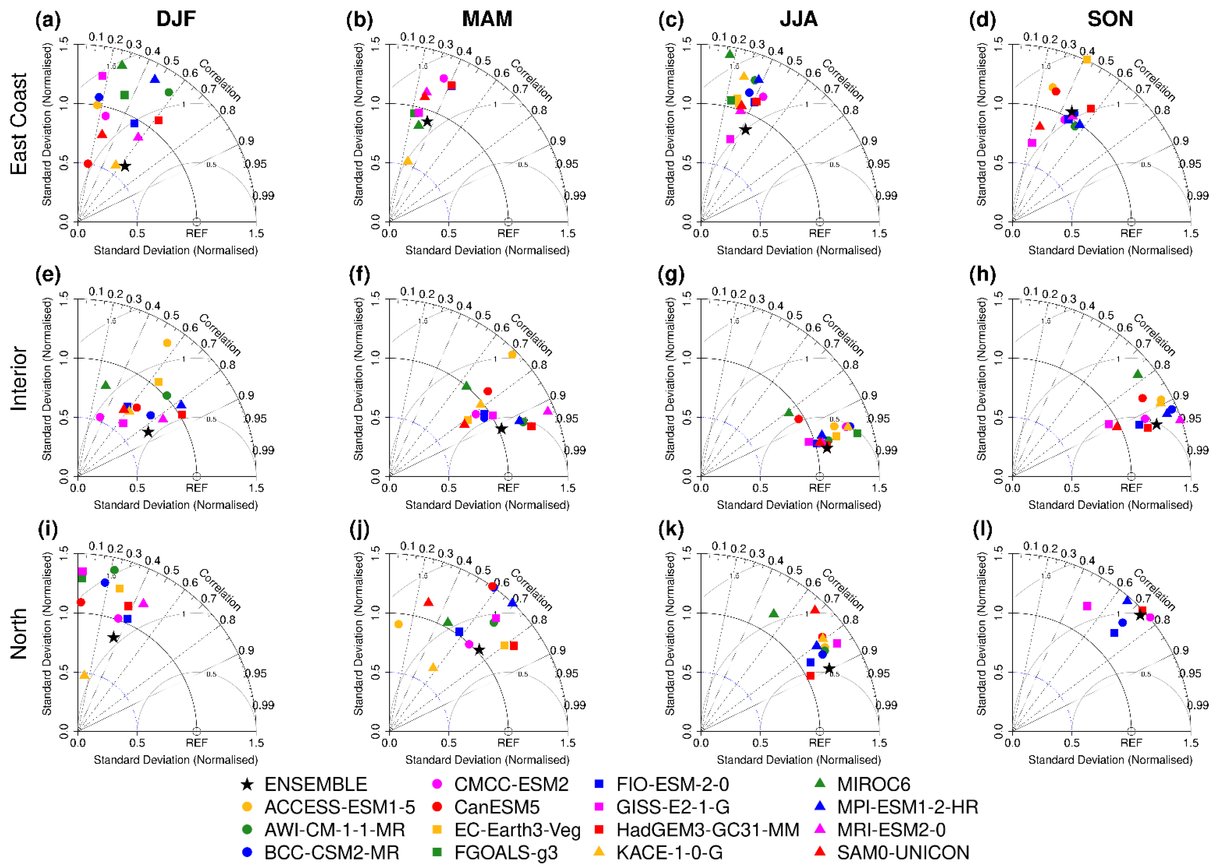
The most representative simulations for precipitation (Figure 6) are observed in June, July, and August (JJA) and September, October, and November (SON) in the Interior and North subregions, compared with December, January, and February (DJF) and March, April, and May (MAM). Compared with the other periods, the best results are found in SON on the East Coast. When analyzed individually, the ensemble performance is better than most models, but it is not the best one. Therefore, we observed that some models have difficulty simulating the seasonal characteristics of rainfall (CRU-TS) at the spatial scale of NEB with greater efficiency.
The ensemble achieved better results in simulating the historical data during JJA and SON. For the East Coast (Figure 6a–d), there is a high standard deviation and a low correlation between the values of the models and the reference more frequently compared with the other subregions analyzed. These results corroborate with the bias analysis (Figure 4), where periods were observed in which the model underestimates and overestimates the reference data. However, some models present superior statistical performance according to the three metrics. The best models are the HadGEM3-GC31-MM, MIROC6, MRI-ESM2-0, SAM0-UNICON, EC-Earth3-Veg, and KACE-1-0-G.
Over the Interior of the NEB (Figure 6e–h), the correlation values are regularly above 0.60, with a low degree of dispersion. This demonstrates the more remarkable ability of the model to capture the seasonal characteristics of this subregion, more specifically for the dry season (JJA) and for the pre-rainy season (SON). Overestimation of precipitation is identified in the rainy season (DJF) and in the austral autumn (MAM). However, there are GCMs in good agreement with the reference point (REF). According to the Taylor diagram, the models with the greatest ability to reproduce seasonal characteristics are the HadGEM3-GC31-MM, SAM0-UNICON, EC-Earth3-Veg, MRI-ESM2-0, ACESS-ESM1-5, FIO-ESM-2-0, and AWI-CM-1-1-MR. The ensemble average showed a superior response to most models in DJF, JJA, and SON.
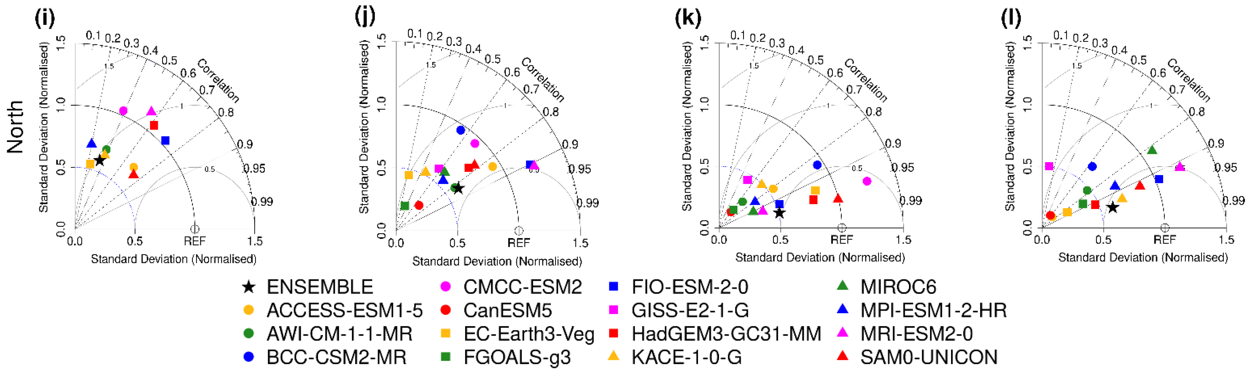
Considering the spatial distribution of rainfall over the northern subregion of NEB (Figure 6i–l), we identified the greater efficiency of the models in simulating rainfall during MAM, JJA, and SON. Due to the underestimation of the variable by the models in DJF, there is a high degree of dispersion highlighted in the Taylor diagram, reducing the ensemble performance during the rainy season. The models that showed the best ability to replicate the spatial behavior of rainfall over the northern NEB are SAM0-UNICON, FIO-ESM2-0, ACCESS-ESM1-5, MRI-ESM2-0, HadGEM3-GC31-MM, EC- Earth3-Veg, and KACE-1-0-G. Figure 6 shows that the ensemble presented good results during MAM, JJA, and SON.
By applying the Taylor diagram, we found the five models that best fit the climatological and spatial characteristics of rainfall for NEB to be HadGEM3-GC31-MM, MRI-ESM2-0, FIO-ESM-2-0, ACCESS-ESM1-5, and EC-Earth3-Veg. During the elaboration of the Taylor diagram, there are times when the results exceed the limits of the graph and, therefore, are not highlighted. It is important to show that the simulations of precipitation by the climate models are a great challenge, due to the great uncertainties associated with the high spatial variability and difficulty in simulating with skill systems, such as ITCZ and SACZ [67]. Therefore, the validation of climate models from databases consolidated by the scientific community, such as the CRU-TS [27], is always recommended [29]. It is known that information from meteorological stations is of fundamental importance in our daily activities as well as in the analysis of climate behavior through scientific research, which provides decision-makers with the best planning of public policies for society. However, spatial data and their quality are frequently limited, as seen in our study area (NEB), where there are few meteorological stations and technical difficulties in keeping them operational. After a robust bibliographical analysis, the CRU-TS version 4 database [57] was selected. It undergoes an efficient interpolation process, where information is used not only on temperature and precipitation but also on seven variables provided by surface stations (mean, minimum, and maximum temperatures; precipitation; vapor pressure; wet days; and cloud cover), thus serving as a reference for validation analyses of CMIP6 models in climate analyses at global and regional levels.
It was verified that the models were more efficient in simulating air temperature data (Figure 7) between the JJA and SON periods for the Interior and North sub-regions. The results indicate superior ability during the austral spring (SON) on the East Coast, as also identified for the precipitation analysis (Figure 6). The CMIP6 ensemble results demonstrate its better performance, in relation to individual models, in capturing the seasonal characteristics of air temperature rather than precipitation. Therefore, in general, the ensemble more efficiently simulates seasonal air temperature patterns in the NEB.
Despite the overall performance, HadGEM3-GC31-MM, MRI-ESM2-0, AWI-CM-1-1-MR, FIO-ESM-2-0, MPI-ESM1-2-HR, GISS-E2-1-G, and the ensemble of all GCMs are ranked as the most skilled according to Taylor diagrams. The Taylor diagrams indicate a high bias of the models in simulating air temperature over the historical period during the four quarters for the East Coast of the NEB (Figure 7a–d). The pattern already observed in the precipitation simulations persists (Figure 6a–d). Temperature underestimation during the annual cycle is most frequently found in CMIP6 models (Figure 5a).
The models have superior skill in relation to the other areas in the Interior, as highlighted in the Taylor diagram (Figure 7e–h). Once again, the model shows a more remarkable ability to capture the seasonal characteristics of this area, as justified by the high correlation values, low RMSE, and the degree of data dispersion close to the reference point. The models can reproduce the seasonal component of climate variability between autumn and austral spring with a more remarkable degree of spatial similarity. The simulations for DJF present a qualitative performance inferior to the other periods, but models with good behavior are recommended for this region. Verifying the model’s ability to simulate the seasonal variability of the air temperature in the Interior shows that the HadGEM3-GC31-MM, MRI-ESM2-0, MPI-ESM1-2-HR, FIO-ESM-2-0, SAM0-UNICON, and AWI-CM-1-1-MR models are the most skillful, according to the semi-qualitative analysis based on Taylor diagrams. The ensemble can reproduce the seasonal variability studied, mainly in the MAM and JJA periods.
Overall, the ensemble of 15 CMIP6 models stands out for how well it simulates climate variability compared with most other models, mainly in MAM. For the North subregion, most CMIP6 models have high standard deviations of air temperature in all seasons due to overestimation relative to the reference point (Figure 7i–l). Significant correlation and moderate RMSE values are observed in the Taylor diagram in MAM, JJA, and SON, justifying the usefulness of the models. HadGEM3-GC31-MM, FIO-ESM2-0, CMCC-ESM2, AWI-CM-1-1-MR, BCC-CSM2-MR, and EC-Earth3-Veg are the GCMs that better reproduce the spatial temperature variability of the subregion.
After validating the models using the Taylor diagram, we found that the top five models with the ability to simulate the spatial variability of air temperature near the surface for NEB are HadGEM3-GC31-MM, FIO-ESM-2-0, MPI-ESM1-2-HR, AWI-CM-1-1-MR, and MRI-ESM2-0.
3.2. Future Climate Change Scenarios
It is shown how the projections for the period 2015–2100 under different scenarios elaborated the use of the ensemble of the 15 models (Figure 8, Figure 9 and Figure 10) and the ensemble of the top 5 models, according to the Taylor diagrams (Figure 11, Figure 12 and Figure 13), for the precipitation and the temperature of the air near the surface. The analysis of the percentage (relative change) projected for the variable precipitation and temperature anomalies (°C) uses the recent period (1980–2014) as a reference.
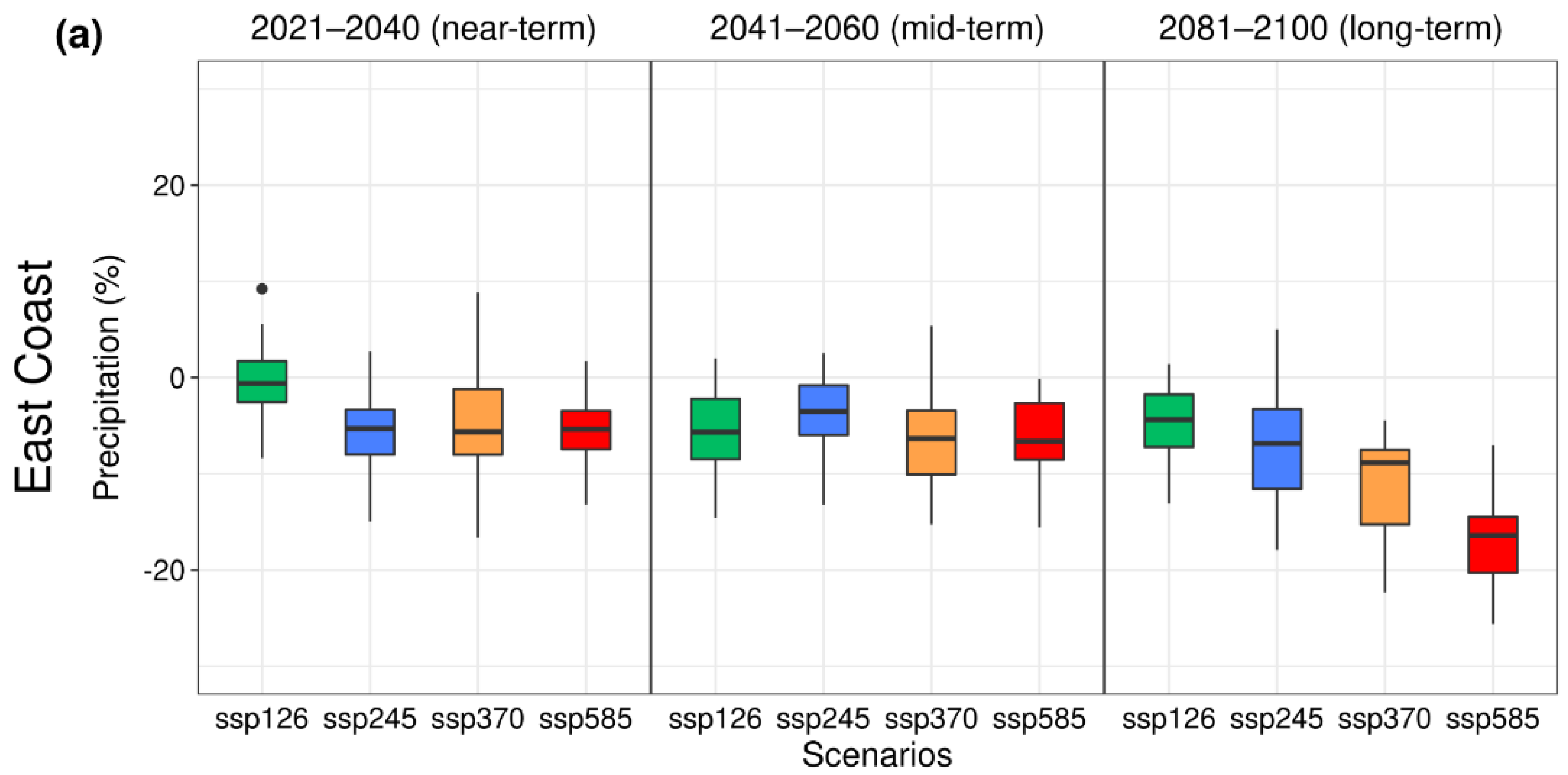
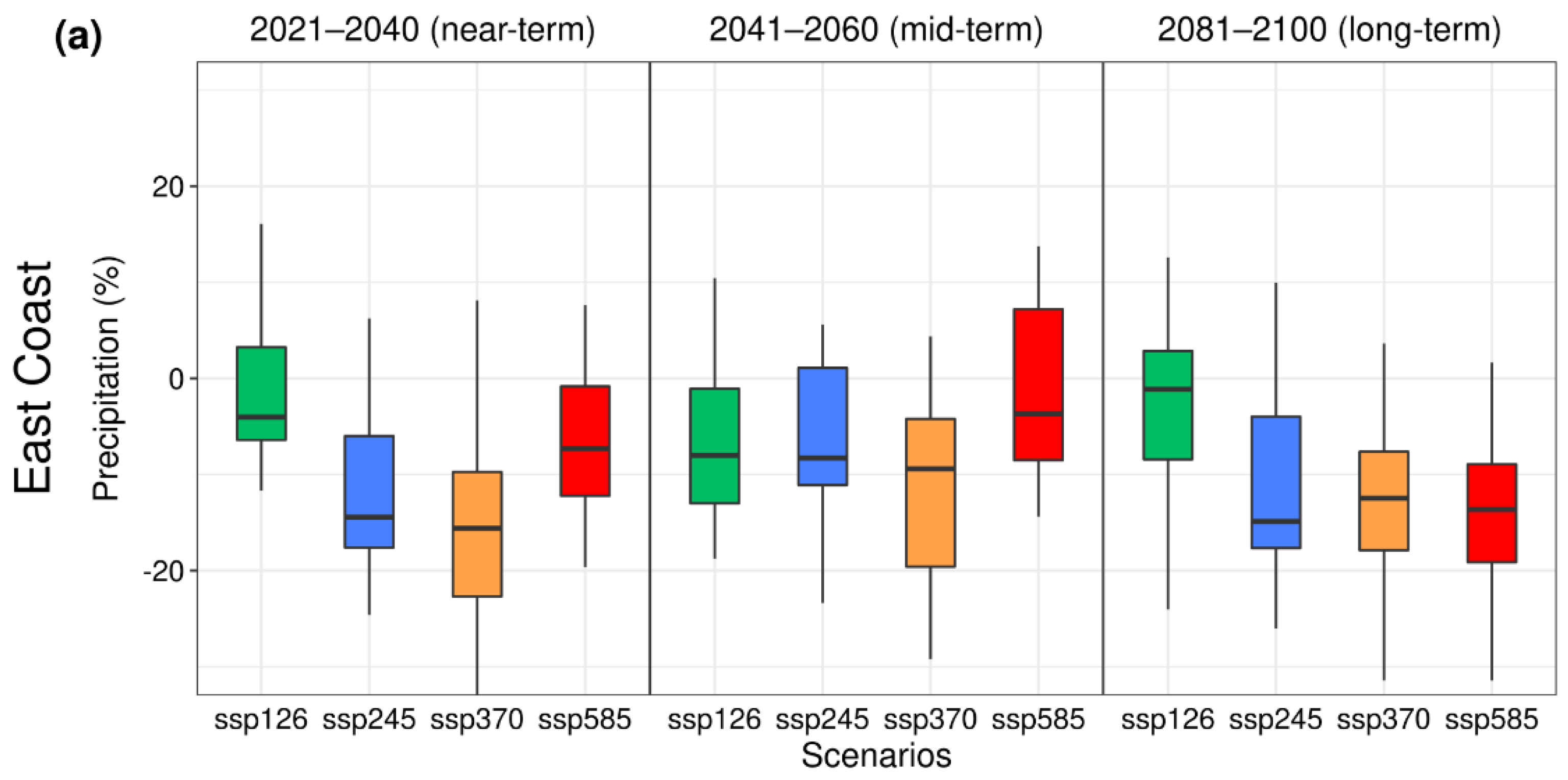
The temporal evolution of the precipitation anomalies for the East Coast (Figure 8a and Figure 9a) shows a decrease in rainfall in both scenarios. The negative trend curve is more evident in the SSP3-7.0 and SSP5-8.5 scenarios in the long-term period. The 15 models (Figure 8a) suggest an annual loss of rainfall greater than −20% until 2100, with a greater chance of extreme climate events, mostly negative, in all scenarios. However, the projections that presented the highest accentuated precipitation deficits correspond to the scenarios of regional rivalry (SSP3-7.0) and development powered by fossil fuels (SSP5-8.5), as seen in Figure 9a. When analyzing the ensemble of the five best models (Figure 11a and Figure 12a), there is high variability in the precipitation projections for the SSP2-4.5, SSP3-7.0, and SSP5-8.5 scenarios. The identified variability, as expected, is higher in relation to the 15 model-based ensemble results, resulting in more significant extremes. The most robust temporal trend is the decrease in annual rainfall. For example, the regional rivalry scenario suggests a reduction of up to 30% of the average for the near-term (2021–2040) (Figure 12a). In the intermediate scenario (SSP2-4.5), the rainfall volume may decrease by up to 27% (long-term). It is essential to highlight that rainfall variability stays around the average (with the deficit) in the sustainable development scenario (SSP1-2.6). Even with outliers with a low rainfall bias, the value remains higher than the lower limits found in the other scenarios (long-term).
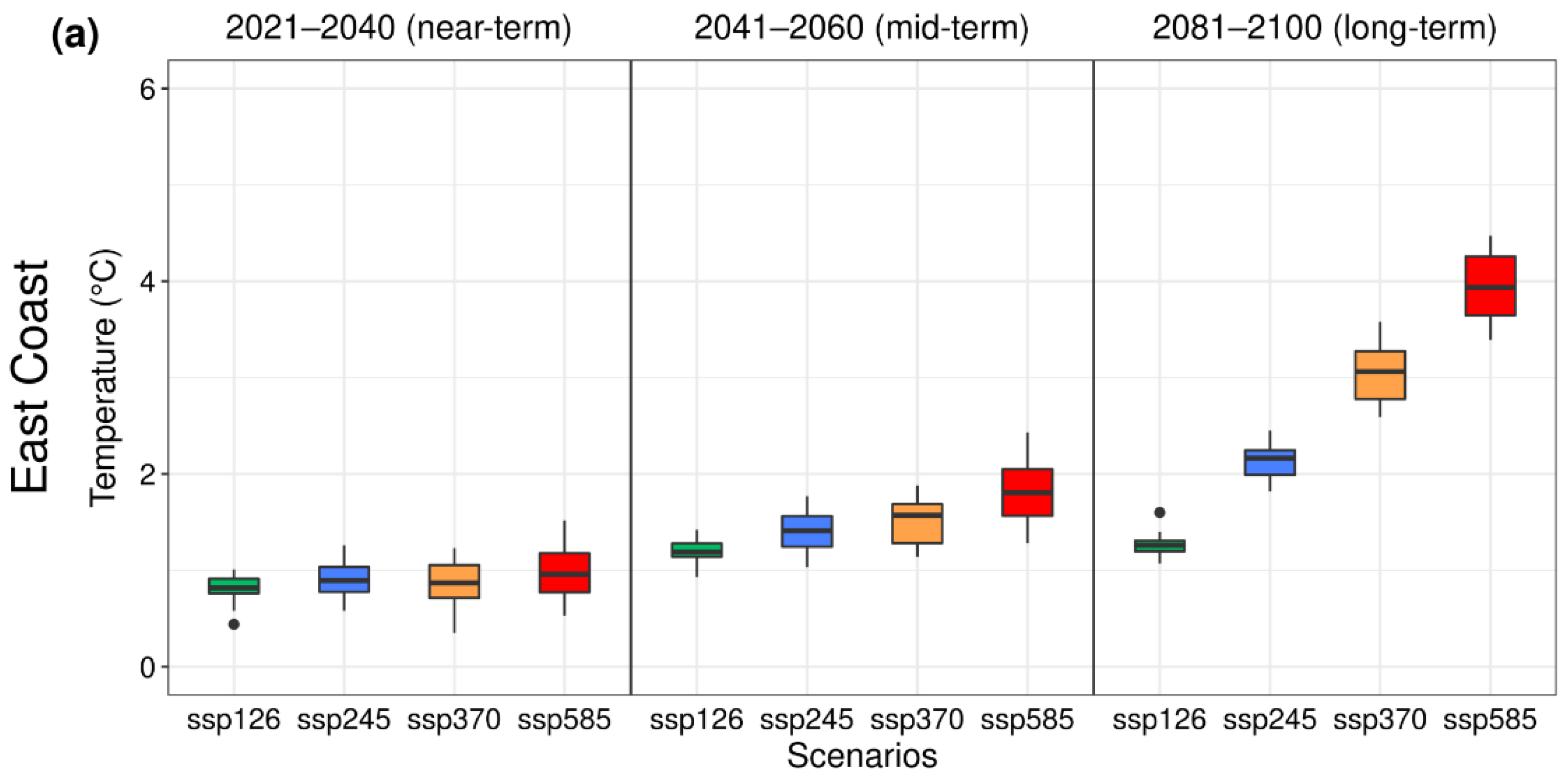
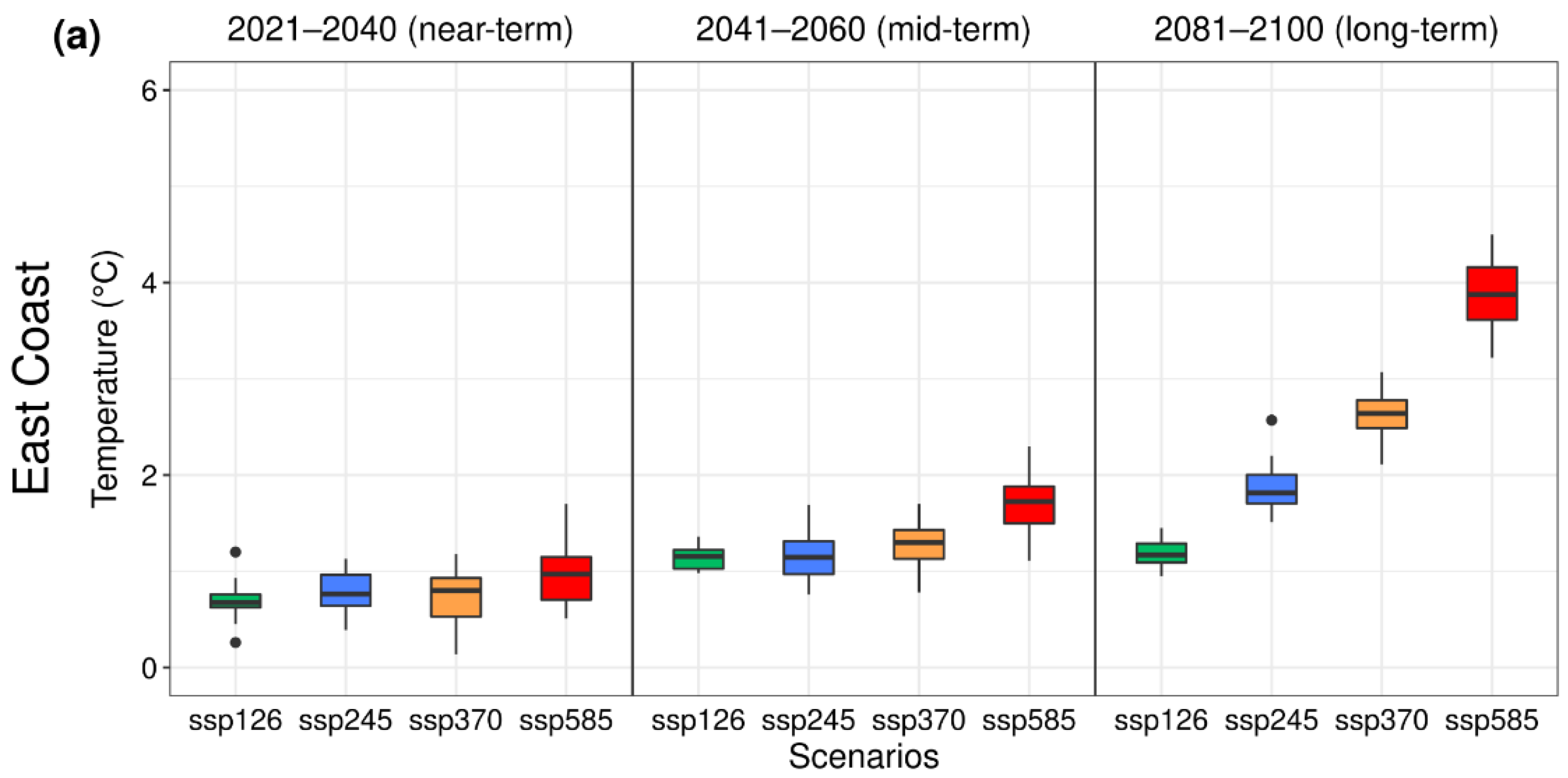
The temporal evolution of air temperature anomalies for the East Coast of NEB for the global (Figure 8b and Figure 10a) and top five (Figure 11b and Figure 13a) model ensembles are very similar. These results indicate an average increase in air temperature in the four scenarios, especially after mid-2040. In the sustainable development scenario (SSP1-2.6), which is the least pessimistic, there is an increase of at least 1 °C in air temperature. An increase of more than 2 °C is projected for the intermediate scenario (SSP2-4.5). The scenario of regional rivalry (SSP3-7.0) suggests temperature increases close to 2 °C in the mid-term and above 3 °C at the end of the century. Temperature increases above 2 °C are projected for mid-century in the fossil-fuel-powered development scenario (SSP5-8.5), exceeding 4 °C by the end of the century. In the global ensemble, we observe that the temperature values are slightly higher than those corresponding to the top 5 models’ ensemble. However, the variability in the top 5 models’ ensemble is higher, resulting in the most positive and negative extreme values.
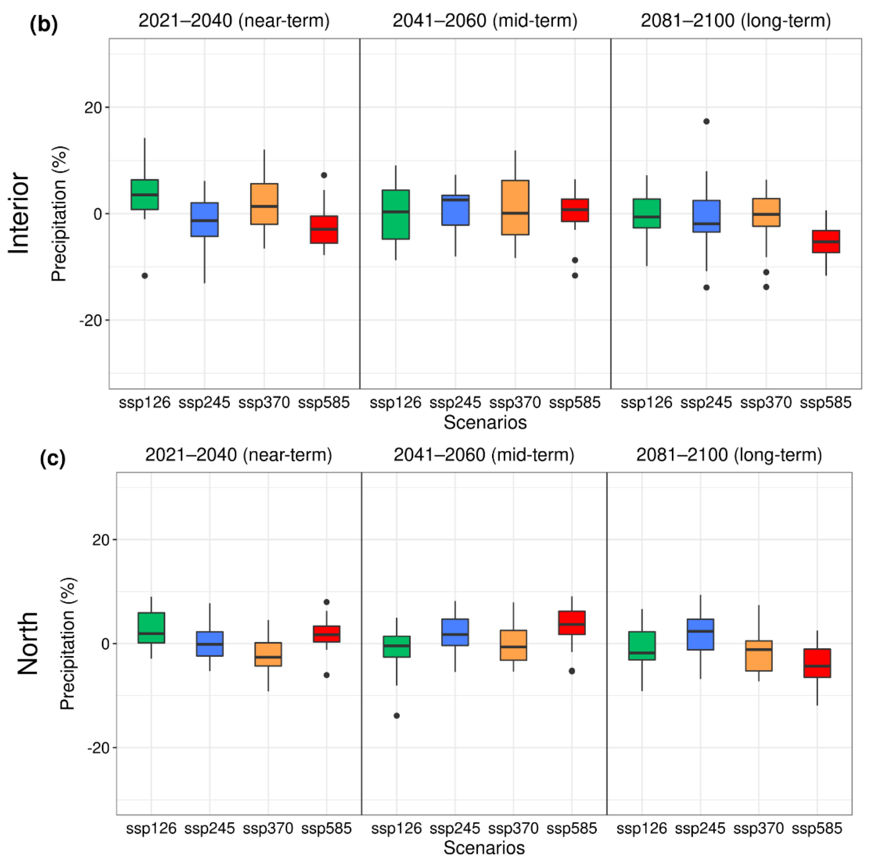
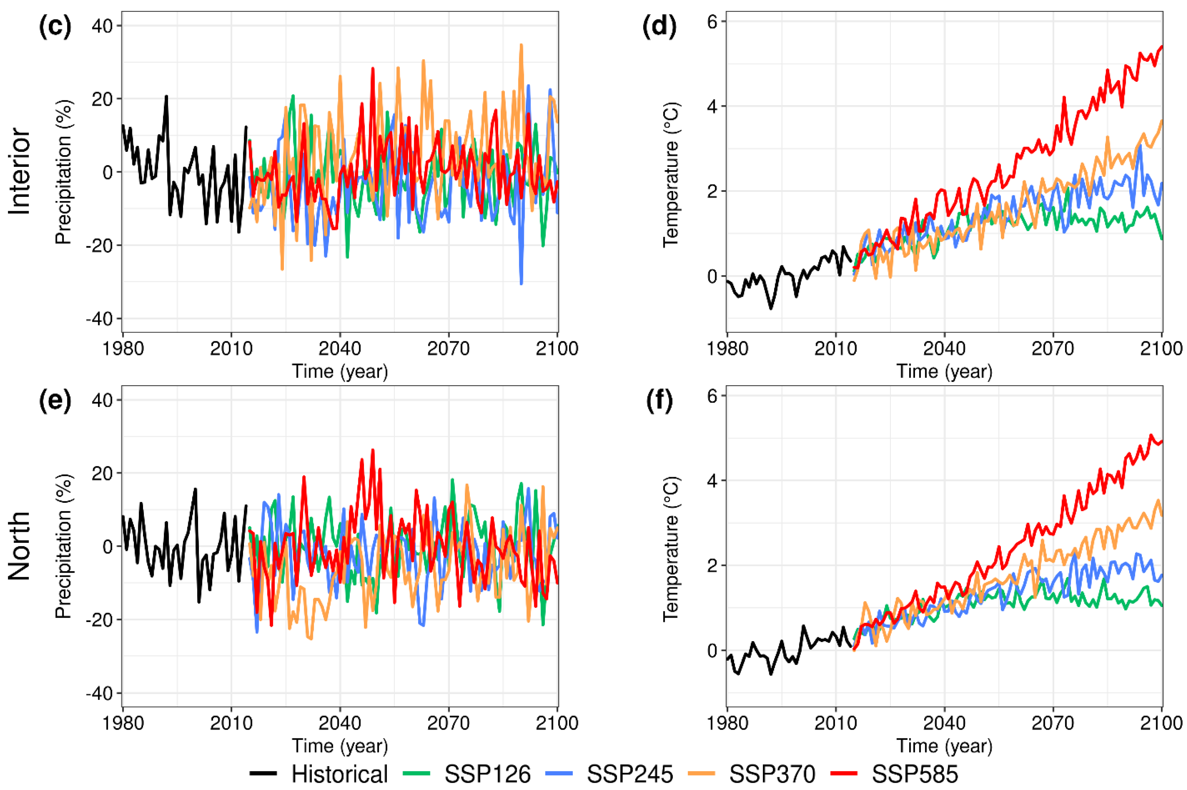
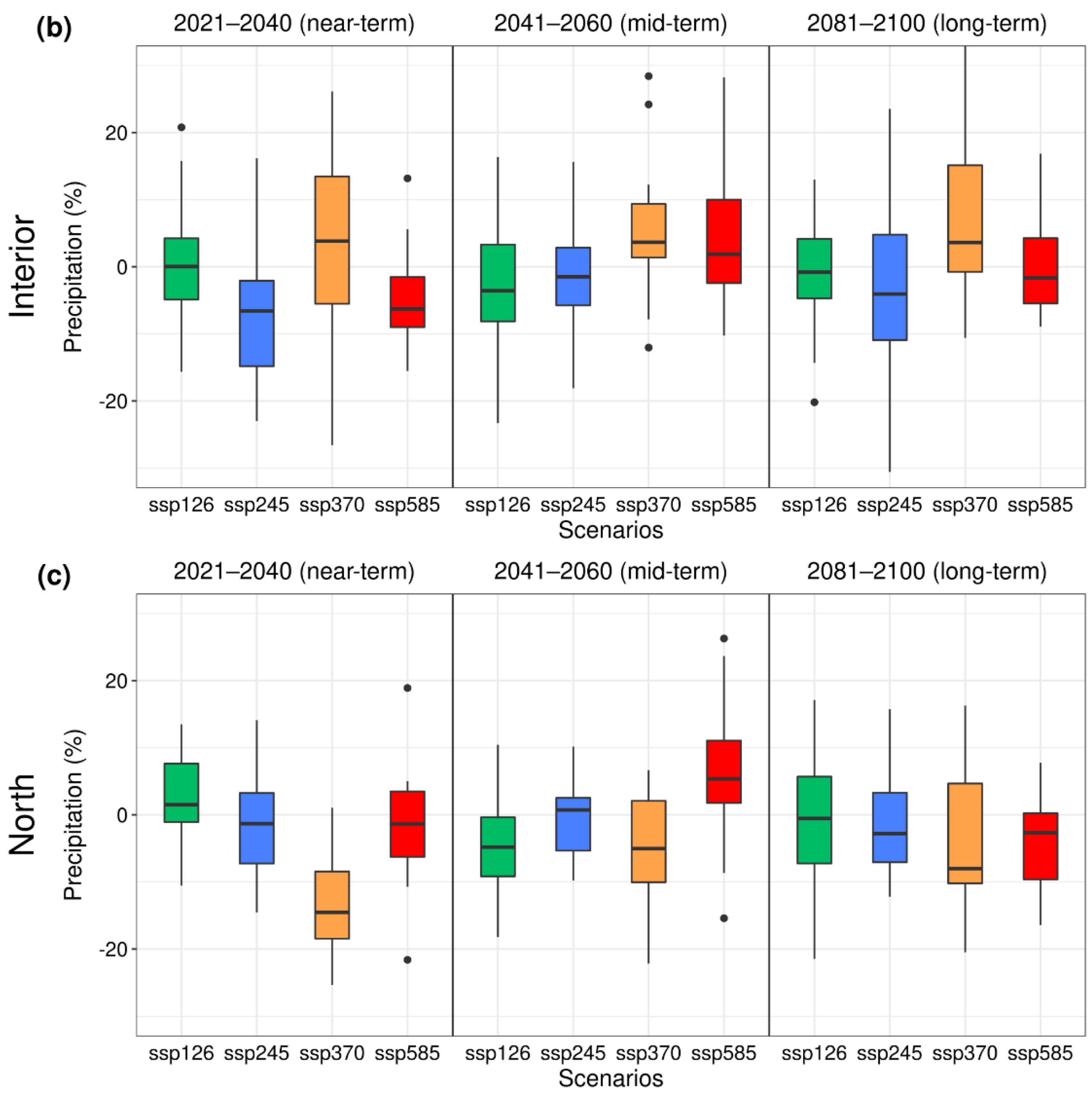
The global ensemble indicates relative changes close to 10%, for all scenarios, in the behavior of precipitation over the Interior of the NEB (Figure 8c and Figure 9b), which suggests an increase or decrease of 10% in the annual total. In the intermediate scenario, extreme high-intensity rainfall events may occur until the end of the century (SSP2-4.5). It is known in the literature that drought events are part of the climatic characteristics of the region; however, these events would be more frequent in the long-term period, as shown in the results of intermediate scenarios (SSP2-4.5), in regional rivalry (SSP3-7.0), and high emissions (SSP5-8.5) scenario results (Figure 9b). The sustainable development scenario (SSP1-2.6) suggests precipitation events with extreme patterns in the coming decades; however, in the middle of the century, the total volume starts to vary close to the climatology. The top 5 model ensemble results (Figure 11c and Figure 12b) show changes in the range of 20%.
The projection for the intermediate scenario (SSP2-4.5) indicates a negative trend in total precipitation in the coming decades (2021–2040). This would again vary in the climatological environment in the mid-term period, and even then, more severe droughts and extreme rainfall are likely to happen. Extreme droughts in the coming decades are identified in the scenario of regional rivalry (SSP3-7.0), which would likely cause water conflicts in the region. Around 2040, an inversion in the trend curve is observed, which becomes positive until the end of the timescale studied. Therefore, in this scenario, there is a greater probability of capturing water resources for the subregions and raising awareness of floods, which already occur frequently. Assuming the current development scenario powered by fossil fuels (SSP5-8.5) remains unchanged, in that case, events followed by droughts will be observed in the coming decade, with above-average rainfall occurring until the mid-term period and stabilizing within the average. In the scenario where the world follows sustainable development (SSP1-2.6), relative change finds a high degree of short-term variability. After this period, the trend predicts rainfall volumes close to climatology, with a drier event close to 2100, corresponding to a probable natural payback period.
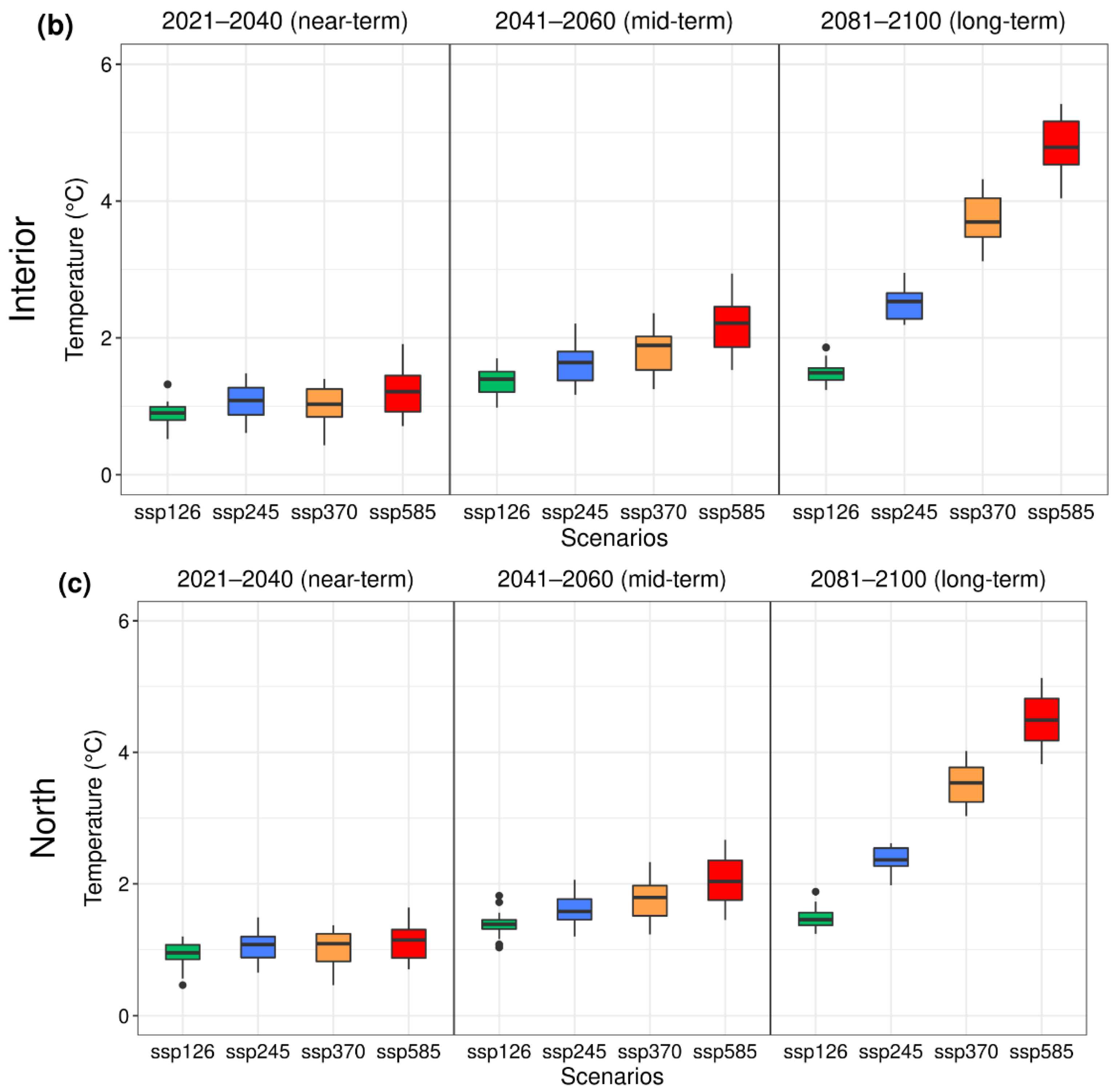
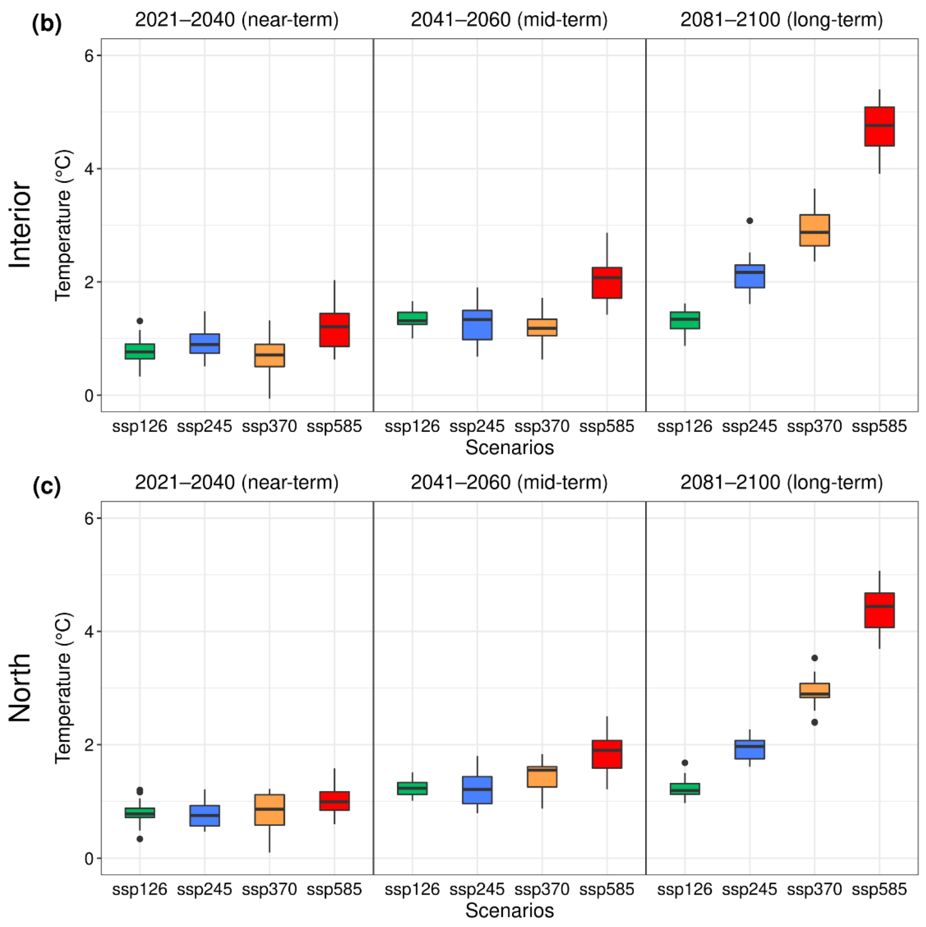
In the Interior region, the global ensemble suggests an average increase in air temperature (Figure 8d and Figure 10b) in all scenarios of at least 1 °C in the near-term period. The projection for the sustainable development scenario (SSP1-2.6) indicates an increase of 1.5 °C between 2041 and 2060, with probable stabilization of this anomaly until the end of the century and no tendency to return to the initial levels. The increase in temperature gains strength in the intermediate scenario (SSP2-4.5). It exceeds and maintains the level of positive anomalies above 2 °C after the mid-term period, with a probable increase of up to 3 °C close to 2100. The intensity of the rises in temperature gains almost linear growth trends, with the climatic forces present in the scenarios of regional rivalry (SSP3-7.0) and development powered by fossil fuels (SSP5-8.5), wherein in the scenario of the dispute (SSP3-7.0), the increase in temperature exceeds 2 °C in 2060 and 4 °C at the end of the century. In the scenario developed with fossil fuels (SSP5-8.5), the growth is more expressive than in the other scenarios, as it presents incredible anomalies of 4 °C in 2080 and, ten years later, exceeds the level of 5 °C.
According to the ensemble of the five best models, an increase in air temperature is projected (Figure 11d and Figure 13b) until the end of the 21st century, similar to the behavior observed and discussed in the global ensemble scenarios. The difference is that the interannual climate variability in the set of the best models is higher and the air temperature increase projection is slightly lower than that found in the global ensemble in the SSP1-2.6, SSP2-4.5, and SSP3-7.0 scenarios.
In the case of precipitation projections over the North subregion of the NEB presented in the global ensemble (Figure 8e and Figure 9c), variability close to 10% in the relative change is identified, with frequent moments of rainfall deficit. The scenario corresponding to sustainable development (SSP1-2.6) suggests that the total annual volume oscillates close to the climatology. In the mid-term and long-term periods, there may be rains 10% below the average expected in the region (extremes) (Figure 9c).
The occurrence of rainfall close to normal but with variation in the lower and upper limits of 10% is verified in the intermediate scenario (SSP2-4.5). The consistency in simulating the sign that a great drought would occur in 2017 is already evident. The characteristics of a world with regional rivalry (SSP3-7.0) are similar to the average of the other scenarios described, but with a slight general decline in total precipitation. The relative change in rainfall is more significant in the high-emissions scenario (SSP5-8.5) than in other scenarios. However, there is a temporal similarity in some decades with the other scenarios; the trend curve would negatively predominate in the long-term period.
The ensemble of the best models suggests high rainfall variability (Figure 11e and Figure 12c) in the 21st century, with a relative change corresponding to a deviation of ±20% in rainfall behavior. This set managed better to simulate the signs of the last recorded droughts. In the sustainable (SSP1-2.6) and intermediate (SSP2-4.5) development scenarios, rainfall variability meets the seasonality characteristic of the region and, therefore, oscillates near the average. Still, we highlight that in the intermediate scenario (SSP2-4.5), there is a greater probability of climatic extremes associated with drought events. There is an assumption that the deficit in the total volume of annual rainfall persists until 2100 in the scenario of regional rivalry (SSP3-7.0), which is more dangerous for the storage of water resources than in the other scenarios presented in Figure 11e. Climate extremes with rainfall decay and an increase of more than 20% (mid-term period) are suggested in the high-emission scenario (SSP5-8.5). It proposes that in the next 50 years, the region will experience severe droughts (near-term period) and extreme rainfall (~2050) and then a decrease in the total expected volume.
For the air temperature over the North of NEB, the scenarios indicate an increase between 1 °C and 5 °C in the two ensembles (global and best models) (Figure 8f, Figure 10c, Figure 11f and Figure 13c). For the sustainable development (SSP1-2.6) environment, the simulations suggest temperatures are still “mild” in the near-term period. However, in the mid-term period, the average temperature would exceed 1 °C, with the strength to reach 2 °C in mid-2050, ranging between these thresholds until 2100. The intermediate scenario (SSP2-4.5) increases the air temperature throughout the entire timescale studied.
In the mid-term period, the anomaly approaches 1.5 °C, with smooth and continuous growth until mid-2090, when it stabilizes with anomalies close to 2.5 °C (Figure 8f and Figure 10c). Continuous and more expressive temperature increases are presented in the scenarios of regional rivalry (SSP3-7.0) and high emissions (SSP5-8.5). In the dispute scenario (SSP3-7.0), the anomalies exceed 2 °C in the mid-term period and approach the 4 °C ceiling at the end of the century. The worst-case scenario (SSP5-8.5) would be an increase of 2 °C in the mid-term period, with potential anomalies of 5 °C in 2100. When we analyze the information presented by the set of best models (Figure 11f and Figure 13c), we observe a more significant interannual variability of temperature anomalies (Figure 11f). The high emission scenario (SSP5-8.5) is similar to the behavior described in the global ensemble. Anomalies close to 1 °C are presented in the most optimistic scenario (SSP1-2.6) in the near-term period (Figure 13c). In the intermediate scenario (SSP2-4.5) temperatures could increase by up to 2 °C in the long term. It does not show a tendency to return to reference standards. The ranking ensemble suggests an increase in temperature in the scenario of more intimate regional rivalry (SSP3-7.0) compared with the global ensemble. Due to this factor, the air temperature anomaly would not reach 4 °C until the end of the 21st century.
4. Discussion
The set of CMIP6 models better simulates the behavior of the variable temperature of the air near the surface than that of precipitation, mainly between December and April. In addition to the characteristics of temperature data (continuous data) and precipitation (discrete data), this may be associated with the high climate variability characteristic of the region, which occurs in different categories of precipitation intensity [3], and the difficulty of GCMs in simulating some meteorological systems, such as the ITCZ and SACZ [68,69]. During this period, the ITCZ is in its southernmost position in its climatology, and it is the primary regulator of rainfall in this region [70,71,72].
As observed by the bias, the annual precipitation cycle simulations in the Interior and North subregions are superior to those found on the East Coast of the NEB. This occurs due to the high precipitation volumes during the austral summer, as simulated by the models for the East Coast. During the rainy season, a high value of bias is found more frequently when compared with the dry season of the respective study areas. Similar results were obtained by [29] when studying CMIP6 simulations in South America. However, in all subregions, some models similarly reproduce the temporal variance of the average rainfall volume in the area. We also highlight the ensemble’s ability and usefulness in simulating precipitation climatology. Another cause of these biases may be the difficulty of CMIP6 models to represent high climate variability due, for example, to their low original resolution and the topography of the analyzed domains [73,74].
The behavior of the rainfall volume in response to climatic forces indicates little change (in general) in the annual average for the North and Interior subregions of the NEB. At the same time, there is a tendency to decrease by approximately 5 to 30% of the annual rainfall volume on the East Coast. Both locations are subject to extreme weather events, mainly droughts, as observed in the outliers (black dots). The air temperature response to climatic forces highlights a tendency to increase in the coming years by at least 1 °C. Even so, in its worst-case scenario (SSP5-8.5), it could exceed 5 °C by 2100.
The projections of the best models (Figure 11) show an average decrease in precipitation with greater intensity and more significant air temperature variability. The positive trend in air temperature is observed to be slightly higher in the global set of CMIP6 (Figure 8, Figure 9 and Figure 10) than in the best models (Figure 11, Figure 12 and Figure 13); analyses were also obtained by [29] when studying climate change over South America. Another important highlight of the sustainable development scenario is that after the mid-term period, the curve of air temperature anomalies tends to approach neutrality slowly, therefore showing a positive response from nature to the concept of sustainability. Therefore, the time to invest in drastic and sustainable change is now [75].
The scenario results may be of great value to inform public sector decisions in guiding a differentiated sustainable development strategy among the three subregions in terms of, for example, infrastructure or water governance. It is essential to establish a reliable early warning system (monitoring and forecasting), promote research in the context of adaptation to extremes, and develop technically sound public policies more adapted to the high variability of the region, aiming for a more resilient society to climate risk.
5. Conclusions
The results presented in this work confirm the efficiency of the CMIP6 models in simulating the climatological pattern of the precipitation and air temperature variables (the best skill), which is generally similar or superior to the CMIP5 models; this is due to the lower bias found in the CMIP6 models, which is provided by improvements in physical processes and greater spatial resolution [76,77,78]. CMIP6 models can also better simulate maximum rainfall values [71].
The Taylor diagram technique proves to be helpful for validating and selecting models with a greater ability to simulate the spatial behavior of variables. This methodology made it possible to identify the HadGEM3-GC31-MM, MRI-ESM2-0, FIO-ESM-2-0, ACCESS-ESM1-5, and EC-Earth3-Veg models as those with the greatest skill in simulating the seasonal characteristics of the precipitation, and the HadGEM3-GC31-MM, FIO-ESM-2-0, MPI-ESM1-2-HR, AWI-CM-1-1-MR, and MRI-ESM2-0 models as the most efficient in simulating seasonal behavior the temperature of the air near the surface.
The CMIP6 GCMs models chosen here efficiently simulate the climatology of precipitation and air temperature near the surface, distinguishing between rainy and dry seasons, which is a feature of NEB. In terms of the global ensemble, it is better at simulating seasonal air temperature characteristics than precipitation. However, due to the systematic biases in the models, underestimation or overestimation is observed. In this context, model validation is essential for developing climate projections with greater confidence. However, it is worth highlighting that, where possible, it is convenient to use observed data rather than global products (e.g., CRU TS).
The air temperature over NEB would irreversibly remain at levels between 1 °C and 5.4 °C above the average of the period of reference, depending on the scenario considered. Overall, the global ensemble suggests an increase in temperature in the SSP1-2.6, SSP2-4.5, and SSP3-7.0 scenarios, higher than those presented in the ranked best models. This temperature rise has, therefore, led to an increase in evaporation and evapotranspiration, which negatively impacts the water volumes of the surface reservoirs and, concurrently, increases the water demand for irrigated agriculture.
The decrease in rainfall is more prominent during the high emission scenario (SSP5-8.5) compared with the other scenarios. Still, it is also likely that the regional rivalry scenario (SSP3-7.0) could cause more climate risk assessments than the high CO2 emission scenario (SSP5-8.5), where the East Coast, which has the most impact on the economy and on the generation of agricultural supplies for the NEB, would experience significant negative impacts on its rainfall regime, with a reduction of up to 30% in its annual volume. This possible impact raises the maximum alert to decision-makers about the increase in frequency, severity, and duration of meteorological droughts. Public policies should be urgently implemented to promote the region’s sustainable development and a more resilient society to climate risk.
GCMs can simulate the historical behavior of the climate variables under study and provide reliable projections. However, the low spatial resolution does not consider local characteristics such as deforestation, fires, soil degradation, erosion, river silting, waste of natural resources, and water contamination. In future activities, daily data from CMIP6 will be used for specific regions of the NEB to verify areas with greater sensitivity to climate risk and assess the characteristics of future extreme events.
Author Contributions
Conceptualization, L.G.D., C.A.C.d.S., C.A.G.S., E.S.P.R.M. and L.M.A.; methodology, L.G.D.; software, L.G.D.; validation, L.G.D.; formal analysis, L.G.D.; investigation, L.G.D., C.A.C.d.S., C.A.G.S., E.S.P.R.M. and L.M.A.; resources, L.G.D.; data curation, L.G.D.; writing—original draft preparation, L.G.D.; writing—review and editing, C.A.C.d.S., C.A.G.S., E.S.P.R.M. and L.M.A.; visualization, L.G.D. and C.A.G.S.; supervision, C.A.C.d.S.; project administration, C.A.C.d.S.; funding acquisition, C.A.C.d.S. All authors have read and agreed to the published version of the manuscript.
Funding
This research was funded by Fundação de Apoio à Pesquisa do Estado da Paraíba (FAPESQPB), through a post-doctoral fellowship to the first author in the scope of the project Study of the Intense Weather Events in Northeastern Brazil (Notice No. 07/2021 SEECT/FAPESQ/PB) and the Graduate Program in Meteorology (PPGMET) of the Federal University of Campina Grande.
Data Availability Statement
CRU TS data are available at the Center for Environmental Data Analysis (CEDA: https://data.ceda.ac.uk//badc/cru/data/cru_ts/, accessed on 25 October 2021) or on the CRU website (https://crudata.uea.ac.uk/cru/data/hrg/, accessed on 25 October 2021) and the CMIP6 models in the Earth System Grid Federation portal (https://esgf-node.llnl.gov/search/cmip6/, accessed on 27 October 2021).
Acknowledgments
We acknowledge the reviewers for their constructive comments and suggestions. We are grateful to the World Climate Research Program’s (WCRP) Working Group on Coupled Modeling and other climate modeling groups worldwide for their dedication to research, development, and the availability of datasets derived from CMIP models. We acknowledge Marcelo Guatura for helping us obtain and process data.
Conflicts of Interest
The authors declare no conflict of interest.
References
- IPCC. “Summary for Policymakers” in Climate Change 2021: The Physical Science Basis. In Contribution of Working Group I to the Sixth Assessment Report of the Intergovernmental Panel on Climate Change; Masson-Delmotte, V., Zhai, P., Pirani, A., Connors, S.L., Péan, C., Chen, Y., Goldfarb, L., Gomis, M.I., Matthews, J.B.R., Berger, S., et al., Eds.; Cambridge University Press: Cambridge, UK, 2021; in press. [Google Scholar]
- Dai, A. Drought under global warming: A review. WIREs Clim. Chang. 2011, 2, 45–65. [Google Scholar] [CrossRef] [Green Version]
- Marengo, J.A.; Torres, R.R.; Alves, L.M. Drought in Northeast Brazil-past, present, and future. Theor. Appl. Climatol. 2017, 129, 1189–1200. [Google Scholar] [CrossRef]
- Ahmed, K.; Shahid, S.; Chung, E.S.; Wang, X.J.; Harun, S.B. Climate change uncertainties in seasonal drought severity-area-frequency curves: Case of arid region of Pakistan. J. Hydrol. 2019, 570, 473–485. [Google Scholar] [CrossRef]
- Huang, J.; Ma, J.; Guan, X.; Li, Y.; He, Y. Progress in semi-arid climate change studies in China. Adv. Atmos. Sci. 2019, 36, 922–937. [Google Scholar] [CrossRef]
- Kousky, V.E. Frontal influences on northeast Brazil. Mon. Weather Rev. 1979, 107, 1140–1153. [Google Scholar] [CrossRef]
- Moura, A.D.; Shukla, J. On the dynamics of droughts in northeast Brazil: Observations, theory and numerical experiments with a general circulation model. J. Atmos. Sci. 1981, 38, 2653–2675. [Google Scholar] [CrossRef]
- Rodrigues, D.T.; Gonçalves, W.A.; Spyrides, M.H.; Santos e Silva, C.M.; Souza, D.O. Spatial distribution of the level of return of extreme precipitation events in Northeast Brazil. Int. J. Climatol. 2020, 40, 5098–5113. [Google Scholar] [CrossRef]
- Uvo, C.B.; Repelli, C.A.; Zebiak, S.E.; Kushnir, Y. The relationships between tropical Pacific and Atlantic SST and northeast Brazil monthly precipitation. J. Clim. 1998, 11, 551–562. [Google Scholar] [CrossRef]
- Hounsou-Gbo, G.A.; Servain, J.; Araujo, M.; Caniaux, G.; Bourlès, B.; Fontenele, D.; Martins, E.S.P. SST indexes in the Tropical South Atlantic for forecasting rainy seasons in Northeast Brazil. Atmosphere 2019, 10, 335. [Google Scholar] [CrossRef] [Green Version]
- Hastenrath, S. Exploring the climate problems of Brazil’s Nordeste: A review. Clim. Chang. 2012, 112, 243–251. [Google Scholar] [CrossRef]
- Utida, G.; Cruz, F.W.; Etourneau, J.; Bouloubassi, I.; Schefuß, E.; Vuille, M.; Novello, V.F.; Prado, L.F.; Sifeddine, A.; Klein, V.; et al. Tropical South Atlantic influence on Northeastern Brazil precipitation and ITCZ displacement during the past 2300 years. Sci. Rep. 2019, 9, 1698. [Google Scholar] [CrossRef] [PubMed] [Green Version]
- Carvalho, L.M.; Jones, C.; Liebmann, B. The South Atlantic convergence zone: Intensity, form, persistence, and relationships with intraseasonal to interannual activity and extreme rainfall. J. Clim. 2004, 17, 88–108. [Google Scholar] [CrossRef]
- Kousky, V.E.; Gan, M.A. Upper tropospheric cyclonic vortices in the tropical South Atlantic. Tellus 1981, 33, 538–551. [Google Scholar] [CrossRef] [Green Version]
- Rodrigues, D.T.; Gonçalves, W.A.; Spyrides, M.H.C.; Andrade, L.D.M.B.; Souza, D.O.; Araujo, P.A.A.; Silva, A.C.N.; Silva, C.M.S. Probability of occurrence of extreme precipitation events and natural disasters in the city of Natal, Brazil. Urban Clim. 2021, 35, 100753. [Google Scholar] [CrossRef]
- Lyra, M.J.A.; Fedorova, N.; Levit, V.; Freitas, I.G.F.D. Characteristics of Mesoscale Convective Complexes over Northeastern Brazil. Rev. Bras. Meteorol. 2020, 35, 727–734. [Google Scholar] [CrossRef]
- Oliveira-Júnior, J.F.; Gois, G.; Lima Silva, I.J.; Oliveira Souza, E.; Jardim, A.M.D.R.F.; Silva, M.V.; Shah, M.; Jamjareegulgarn, P. Wet and dry periods in the state of Alagoas (Northeast Brazil) via Standardized Precipitation Index. JASTP 2021, 224, 105746. [Google Scholar] [CrossRef]
- Cavalcanti, I.F. Tempo e Clima no Brasil; Oficina de Textos: São Paulo, Brasil, 2016. [Google Scholar]
- Brito, S.S.B.; Cunha, A.P.M.; Cunningham, C.C.; Alvalá, R.C.; Marengo, J.A.; Carvalho, M.A. Frequency, duration and severity of drought in the Semiarid Northeast Brazil region. Int. J. Climatol. 2018, 38, 517–529. [Google Scholar] [CrossRef]
- Marengo, J.A.; Cunha, A.P.M.; Nobre, C.A.; Neto, G.G.R.; Magalhaes, A.R.; Torres, R.R.; Sampaio, G.; Alexandre, F.; Alves, L.M.; Cuartas, L.A.; et al. Assessing drought in the drylands of northeast Brazil under regional warming exceeding 4 C. Nat. Hazards 2020, 103, 2589–2611. [Google Scholar] [CrossRef]
- Hastenrath, S. Interannual variability and annual cycle: Mechanisms of circulation and climate in the tropical Atlantic. Mon. Weather Rev. 1984, 112, 1097–1107. [Google Scholar] [CrossRef]
- Kayano, M.T.; Andreoli, R.V. Decadal variability of northern northeast Brazil rainfall and its relation to tropical sea surface temperature and global sea level pressure anomalies. J. Geophys. Res. Oceans 2004, 109, C11011. [Google Scholar] [CrossRef]
- Santos, S.R.Q.; Cunha, A.P.M.A.; Ribeiro-Neto, G.G. Avaliação de dados de precipitação para o monitoramento do padrão espaço-temporal da seca no nordeste do Brasil. Rev. Bras. Climatol. 2019, 25, 80–100. [Google Scholar] [CrossRef] [Green Version]
- Pereira, M.P.S.; Mendes, K.R.; Justino, F.; Couto, F.; Silva, A.S.; Silva, D.F.; Malhado, A.C.M. Brazilian dry forest (Caatinga) response to multiple ENSO: The role of Atlantic and Pacific Ocean. Sci. Total Environ. 2020, 705, 135717. [Google Scholar] [CrossRef] [PubMed]
- Kane, R.P. Prediction of droughts in north-east Brazil: Role of ENSO and use of periodicities. Int. J. Climatol. 1997, 17, 655–665. [Google Scholar] [CrossRef]
- Langenbrunner, B. Water, water not everywhere. Nat. Clim. Chang. 2021, 11, 650. [Google Scholar] [CrossRef]
- Rivera, J.A.; Arnould, G. Evaluation of the ability of CMIP6 models to simulate precipitation over Southwestern South America: Climatic features and long-term trends (1901–2014). Atmos. Res. 2020, 241, 104953. [Google Scholar] [CrossRef]
- Bustos Usta, D.F.; Teymouri, M.; Chatterjee, U. Projections of temperature changes over South America during the twenty-first century using CMIP6 models. GeoJournal 2021, 87, 739–763. [Google Scholar] [CrossRef]
- Ortega, G.; Arias, P.A.; Villegas, J.C.; Marquet, P.A.; Nobre, P. Present-day and future climate over central and South America according to CMIP5/CMIP6 models. Int. J. Climatol. 2021, 41, 6713–6735. [Google Scholar] [CrossRef]
- Almazroui, M.; Ashfaq, M.; Islam, M.N.; Rashid, I.U.; Kamil, S.; Abid, M.A.; O’Brien, E.; Ismail, M.; Reboita, M.S.; Sörensson, A.A.; et al. Assessment of CMIP6 Performance and Projected Temperature and Precipitation Changes Over South America. Earth Syst. Environ. 2021, 5, 155–183. [Google Scholar] [CrossRef]
- Alves, L.M.; Chadwick, R.; Moise, A.; Brown, J.; Marengo, J.A. Assessment of rainfall variability and future change in Brazil across multiple timescales. Int. J. Climatol. 2021, 41, E1875–E1888. [Google Scholar] [CrossRef]
- Gomes, H.B.; Lemos da Silva, M.C.; Barbosa, H.M.J.; Ambrizzi, T.; Baltaci, H.; Gomes, H.B.; Silva, F.D.S.; Costa, R.L.; Figueroa, S.N.; Herdies, D.L.; et al. WRF Sensitivity for Seasonal Climate Simulations of Precipitation Fields on the CORDEX South America Domain. Atmosphere 2022, 13, 107. [Google Scholar] [CrossRef]
- Fan, X.; Duan, Q.; Shen, C.; Wu, Y.; Xing, C. Global surface air temperatures in CMIP6: Historical performance and future changes. Environ. Res. Lett. 2020, 15, 104056. [Google Scholar] [CrossRef]
- Ajjur, S.B.; Al-Ghamdi, S.G. Global hotspots for future absolute temperature extremes from CMIP6 models. Earth Space Sci. 2021, 8, e2021EA001817. [Google Scholar] [CrossRef]
- Eyring, V.; Bony, S.; Meehl, G.A.; Senior, C.A.; Stevens, B.; Stouffer, R.J.; Taylor, K.E. Overview of the Coupled Model Intercomparison Project Phase 6 (CMIP6) experimental design and organization. Geosci. Model Dev. 2016, 9, 1937–1958. [Google Scholar] [CrossRef] [Green Version]
- Zhu, H.; Jiang, Z.; Li, J.; Li, W.; Sun, C.; Li, L. Does CMIP6 inspire more confidence in simulating climate extremes over China? Adv. Atmos. Sci. 2020, 37, 1119–1132. [Google Scholar] [CrossRef]
- Meehl, G.A.; Boer, G.J.; Covey, C.; Latif, M.; Stouffer, R.J. The coupled model intercomparison project (CMIP). Bull. Am. Meteorol. Soc. 2000, 81, 313–318. [Google Scholar] [CrossRef]
- Meehl, G.A.; Covey, C.; Taylor, K.E.; Delworth, T.; Stouffer, R.J.; Latif, M.; McAvaney, B.; Mitchell, J.F.B. THE WCRP CMIP3 Multimodel Dataset: A New Era in Climate Change Research. Bull. Am. Meteorol. Soc. 2007, 88, 1383–1394. [Google Scholar] [CrossRef] [Green Version]
- Taylor, K.E.; Stouffer, R.J.; Meehl, G.A. An Overview of Cmip5 and the Experiment Design. Bull. Am. Meteorol. Soc. 2012, 93, 485–498. [Google Scholar] [CrossRef] [Green Version]
- Eyring, V.; Bock, L.; Lauer, A.; Righi, M.; Schlund, M.; Andela, B.; Arnone, E.; Bellprat, O.; Brötz, B.; Caron, L.-P.; et al. ESMValTool v2.0 Extended set of large-scale diagnostics for quasi-operational and comprehensive evaluation of Earth system models in CMIP. Geosci. Model Dev. 2020, 13, 3384–3438. [Google Scholar] [CrossRef]
- Riahi, K.; Van Vuuren, D.P.; Kriegler, E.; Edmonds, J.; O’neill, B.C.; Fujimori, S.; Bauer, N.; Calvin, K.; Dellink, R.; Fricko, O.; et al. The shared socioeconomic pathways and their energy, land use, and greenhouse gas emissions implications: An overview. Glob. Environ. Chang. 2017, 42, 153–168. [Google Scholar] [CrossRef] [Green Version]
- Chen, G.; Li, X.; Liu, X.; Chen, Y.; Liang, X.; Leng, J.; Xu, X.; Liao, W.; Qiu, Y.; Wu, Q.; et al. Global projections of future urban land expansion under shared socioeconomic pathways. Nat. Commun. 2020, 11, 537. [Google Scholar] [CrossRef]
- Gütschow, J.; Jeffery, M.L.; Günther, A.; Meinshausen, M. Country-resolved combined emission and socio-economic pathways based on the Representative Concentration Pathway (RCP) and Shared Socio-Economic Pathway (SSP) scenarios. Earth Syst. Sci. Data 2021, 13, 1005–1040. [Google Scholar] [CrossRef]
- Meehl, G.A.; Senior, C.A.; Eyring, V.; Flato, G.; Lamarque, J.F.; Stouffer, R.J.; Taylor, K.E.; Schlund, M. Context for interpreting equilibrium climate sensitivity and transient climate response from the CMIP6 Earth system models. Sci. Adv. 2020, 6, eaba1981. [Google Scholar] [CrossRef] [PubMed]
- Magalhães, A.R. Life and Drought in Brazil. In Drought in Brazil: Proactive Management and Policy; De Nys, E., Engle, N., Magalhães, A.R., Eds.; Taylor & Francis: Boca Raton, FL, USA, 2016; Chapter 1; pp. 1–18. [Google Scholar]
- Wainwright, C.M.; Black, E.; Allan, R.P. Future changes in wet and dry season characteristics in CMIP5 and CMIP6 simulations. J. Hydrometeorol. 2021, 22, 2339–2357. [Google Scholar] [CrossRef]
- Srivastava, A.; Grotjahn, R.; Ullrich, P.A. Evaluation of historical CMIP6 model simulations of extreme precipitation over contiguous US regions. Weather Clim. Extrem. 2020, 29, 100268. [Google Scholar] [CrossRef]
- Klutse, N.A.B.; Quagraine, K.A.; Nkrumah, F.; Quagraine, K.T.; Berkoh-Oforiwaa, R.; Dzrobi, J.F.; Sylla, M.B. The climatic analysis of summer monsoon extreme precipitation events over West Africa in CMIP6 simulations. Earth Syst. Environ. 2021, 5, 25–41. [Google Scholar] [CrossRef]
- Wang, Y.C.; Hsu, H.H.; Chen, C.A.; Tseng, W.L.; Hsu, P.C.; Lin, C.W.; Chen, Y.L.; Jiang, L.C.; Lee, Y.C.; Liang, H.C.; et al. Performance of the Taiwan Earth System Model in Simulating Climate Variability Compared with Observations and CMIP6 Model Simulations. J. Adv. Model. Earth Syst. 2021, 13, e2020MS002353. [Google Scholar] [CrossRef]
- Volodin, E.; Gritsun, A. Simulation of observed climate changes in 1850–2014 with climate model INM-CM5. Earth Syst. Dyn. 2018, 9, 1235–1242. [Google Scholar] [CrossRef] [Green Version]
- Yuan, S.; Quiring, S.M.; Leasor, Z.T. Historical changes in surface soil moisture over the contiguous United States: An assessment of CMIP6. Geophys. Res. Lett. 2020, 47, e2020GL089991. [Google Scholar] [CrossRef]
- Cos, J.; Doblas-Reyes, F.; Jury, M.; Marcos, R.; Bretonnière, P.A.; Samsó, M. The Mediterranean climate change hotspot in the CMIP5 and CMIP6 projections. Earth Syst. Dyn. 2022, 13, 321–340. [Google Scholar] [CrossRef]
- Lehtonen, H.S.; Aakkula, J.; Fronzek, S.; Helin, J.; Hildén, M.; Huttunen, S.; Kaljonen, M.; Niemi, J.; Palosuo, T.; Pirttioja, N.; et al. Shared socioeconomic pathways for climate change research in Finland: Co-developing extended SSP narratives for agriculture. Reg. Environ. Chang. 2021, 21, 7. [Google Scholar] [CrossRef]
- Knutti, R.; Sedláček, J. Robustness and uncertainties in the new CMIP5 climate model projections. Nat. Clim. Chang. 2013, 3, 369–373. [Google Scholar] [CrossRef]
- Gao, J.; Sheshukov, A.Y.; Yen, H.; Douglas-Mankin, K.R.; White, M.J.; Arnold, J.G. Uncertainty of hydrologic processes caused by bias-corrected CMIP5 climate change projections with alternative historical data sources. J. Hydrol. 2019, 568, 551–561. [Google Scholar] [CrossRef]
- Harris, I.; Jones, P.D.; Osborn, T.J.; Lister, D.H. Updated high-resolution grids of monthly climatic observations—The CRU TS3.10 Dataset. Int. J. Climatol. 2014, 34, 623–642. [Google Scholar] [CrossRef] [Green Version]
- Harris, I.; Osborn, T.J.; Jones, P.; Lister, D. Version 4 of the CRU TS monthly high-resolution gridded multivariate climate dataset. Sci. Data. 2020, 7, 109. [Google Scholar] [CrossRef] [PubMed] [Green Version]
- Ngoma, H.; Wen, W.; Ayugi, B.; Babaousmail, H.; Karim, R.; Ongoma, V. Evaluation of precipitation simulations in CMIP6 models over Uganda. Int. J. Climatol. 2021, 41, 4734–4768. [Google Scholar] [CrossRef]
- Taylor, K.E. Summarizing multiple aspects of model performance in a single diagram. J. Geophys. Res. Atmos. 2001, 106, 7183–7192. [Google Scholar] [CrossRef]
- Kim, Y.H.; Min, S.K.; Zhang, X.; Sillmann, J.; Sandstad, M. Evaluation of the CMIP6 multi-model ensemble for climate extreme indices. Weather. Clim. Extrem. 2020, 29, 100269. [Google Scholar] [CrossRef]
- Díaz, L.B.; Saurral, R.I.; Vera, C.S. Assessment of South America summer rainfall climatology and trends in a set of global climate models large ensembles. Int. J. Climatol. 2021, 41, E59–E77. [Google Scholar] [CrossRef]
- Fotso-Nguemo, T.C.; Chamani, R.; Yepdo, Z.D.; Sonkoué, D.; Matsaguim, C.N.; Vondou, D.A.; Tanessong, R.S. Projected trends of extreme rainfall events from CMIP5 models over Central Africa. Atmos. Sci. Lett. 2018, 19, e803. [Google Scholar] [CrossRef]
- Kumar, D.; Kodra, E.; Ganguly, A.R. Regional and seasonal intercomparison of CMIP3 and CMIP5 climate model ensembles for temperature and precipitation. Clim. Dyn. 2014, 43, 2491–2518. [Google Scholar] [CrossRef]
- Ongoma, V.; Chen, H.; Gao, C. Evaluation of CMIP5 twentieth century rainfall simulation over the equatorial East Africa. Theor. Appl. Climatol. 2019, 135, 893–910. [Google Scholar] [CrossRef]
- Lu, X.; Rao, X.; Dong, W. Model evaluation and uncertainties in projected changes of drought over northern China based on CMIP5 models. Int. J. Climatol. 2021, 41, E3085–E3100. [Google Scholar] [CrossRef]
- Zhao, T.; Chen, L.; Ma, Z. Simulation of historical and projected climate change in arid and semiarid areas by CMIP5 models. Chin. Sci. Bull. 2014, 59, 412–429. [Google Scholar] [CrossRef]
- Firpo, M.A.F.; Guimarães, B.S.; Dantas, L.G.; Silva, M.G.B.; Alves, L.M.; Chadwick, R.; Llopart, M.P.; Oliveira, G.S. Assessment of CMIP6 models’ performance in simulating present-day climate in Brazil. Front. Clim. 2022, 4, 948499. [Google Scholar] [CrossRef]
- Villamayor, J.; Ambrizzi, T.; Mohino, E. Influence of decadal sea surface temperature variability on northern Brazil rainfall in CMIP5 simulations. Clim. Dyn. 2018, 51, 563–579. [Google Scholar] [CrossRef]
- Cavalcanti, I.F.; Silveira, V.P.; Figueroa, S.N.; Kubota, P.Y.; Bonatti, J.P.; Souza, D.C. Climate variability over South America-regional and large scale features simulated by the Brazilian Atmospheric Model (BAM-v0). Int. J. Climatol. 2020, 40, 2845–2869. [Google Scholar] [CrossRef]
- Hastenrath, S.; Heller, L. Dynamics of climatic hazards in northeast Brazil. Q. J. R. Meteorol. Soc. 1977, 103, 77–92. [Google Scholar] [CrossRef]
- Schneider, T.; Bischoff, T.; Haug, G. Migrations and dynamics of the intertropical convergence zone. Nature 2014, 513, 45–53. [Google Scholar] [CrossRef]
- Medeiros, F.J.; Oliveira, C.P.; Torres, R.R. Climatic aspects and vertical structure circulation associated with the severe drought in Northeast Brazil (2012–2016). Clim. Dyn. 2020, 55, 2327–2341. [Google Scholar] [CrossRef]
- Lv, Y.; Guo, J.; Yim, S.H.L.; Yun, Y.; Yin, J.; Liu, L.; Zhang, Y.; Yang, Y.; Yan, T.; Chen, D. Towards understanding multi-model precipitation predictions from CMIP5 based on China hourly merged precipitation analysis data. Atmos. Res. 2020, 231, 104671. [Google Scholar] [CrossRef]
- Yazdandoost, F.; Moradian, S.; Izadi, A.; Aghakouchak, A. Evaluation of CMIP6 precipitation simulations across different climatic zones: Uncertainty and model intercomparison. Atmos. Res. 2021, 250, 105369. [Google Scholar] [CrossRef]
- IPCC. “Summary for policymakers” in Climate Change 2022: Impacts, Adaptation, and Vulnerability. In Contribution of Working Group II to the Sixth Assessment Report of the Intergovernmental Panel on Climate Change; Pörtner, H.-O., Roberts, D.C., Tignor, M., Poloczanska, E.S., Mintenbeck, K., Alegría, A., Craig, M., Langsdorf, S., Löschke, S., Möller, V., Eds.; Cambridge University Press: Cambridge, UK, 2022; in press. [Google Scholar]
- Seneviratne, S.I.; Hauser, M. Regional climate sensitivity of climate extremes in CMIP6 versus CMIP5 multimodel ensembles. Earths Future 2020, 8, e2019EF001474. [Google Scholar] [CrossRef] [PubMed]
- Li, J.L.; Xu, K.M.; Jiang, J.H.; Lee, W.L.; Wang, L.C.; Yu, J.Y.; Stephens, G.; Fetzer, E.; Wang, Y.H. An overview of CMIP5 and CMIP6 simulated cloud ice, radiation fields, surface wind stress, sea surface temperatures, and precipitation over tropical and subtropical oceans. J. Geophys. Res. Atmos. 2020, 125, e2020JD032848. [Google Scholar] [CrossRef]
- Tian, B.; Dong, X. The double ITCZ bias in CMIP3, CMIP5, and CMIP6 models based on annual mean precipitation. Geophys. Res. Lett. 2020, 47, e2020GL087232. [Google Scholar] [CrossRef]
Figure 1.
Northeastern Brazil and the three subregions used in this study: East Coast, Interior, and North.
Figure 1.
Northeastern Brazil and the three subregions used in this study: East Coast, Interior, and North.

Figure 2.
Flowchart illustrating the steps applied in this study to obtain projections of climate change scenarios.
Figure 2.
Flowchart illustrating the steps applied in this study to obtain projections of climate change scenarios.

Figure 3.
Annual cycle of average precipitation and temperature over subregions along the East Coast (a,b), Interior (c,d), and North (e,f) of the NEB, based on the reference period (1980–2014). The 15 CMIP6 models are highlighted by the gray line, the ensemble line in red, and the reference data (CRU-TS) line in black.

Figure 4.
Annual cycle of average precipitation over subregions (a) East Coast, (b) Interior, and (c) North of NEB, based on the reference period (1980–2014).
Figure 4.
Annual cycle of average precipitation over subregions (a) East Coast, (b) Interior, and (c) North of NEB, based on the reference period (1980–2014).

Figure 5.
Annual cycle of mean surface air temperature over subregions (a) East Coast, (b) Interior, and (c) North of the NEB, based on the reference period (1980–2014).
Figure 5.
Annual cycle of mean surface air temperature over subregions (a) East Coast, (b) Interior, and (c) North of the NEB, based on the reference period (1980–2014).


Figure 6.
Taylor diagram analysis of seasonal precipitation averaged over the East Coast (a–d), Interior (e–h), and North (i–l) of NEB for 15 CMIP6 models in DJF (first column), MAM (second column), JJA (third column), and SON (fourth column). The term “REF” indicates the reference data from 1980 to 2014.


Figure 7.
Taylor diagram analysis of seasonal near-surface air temperature averaged over the East Coast (a–d), Interior (e–h), and North (i–l) of the NEB, for 15 CMIP6 models in DJF (first column), MAM (second column), JJA (third column), and SON (fourth column). The term “REF” indicates the reference data from 1980 to 2014.

Figure 8.
Projections of total annual precipitation anomalies (%) and air temperature near the surface (°C) on NEB relative to the reference period (1980–2014): (a,b) East Coast, (c,d) Interior, and (e,f) North. The colored lines correspond to the average of the 15 models (ensemble) of CMIP6 for the SSP1-2.6, SSP2-4.5, SSP3-7.0, and SSP5-8.5 scenarios.

Figure 9.
Boxplot of the relative change in precipitation for the near-term, mid-term, and long-term (end of the century) periods: (a) East Coast, (b) Interior, and (c) North. The colored box plot corresponds to the average of the 15 models (ensemble) of CMIP6 for the SSP1-2.6, SSP2-4.5, SSP3-7.0, and SSP5-8.5 scenarios.


Figure 10.
Boxplot of the air temperature anomaly CMIP6 for the near-term, mid-term, and long-term (end of the century) period: (a) East Coast, (b) Interior, and (c) North. The colored box plot corresponds to the average of the 15 models (ensemble) of CMIP6 for the SSP1-2.6, SSP2-4.5, SSP3-7.0, and SSP5-8.5 scenarios.


Figure 11.
Projections of total annual precipitation anomalies (%) and air temperature near the surface (°C) on NEB relative to the reference period (1980–2014): (a,b) East Coast, (c,d) Interior, and (e,f) North. The colored lines correspond to the average of the 5 best models (ensemble) of CMIP6 for the SSP1-2.6, SSP2-4.5, SSP3-7.0, and SSP5-8.5 scenarios.


Figure 12.
Boxplot of the relative change in precipitation CMIP6 for the near-term, mid-term, and long-term (end of the century) period: (a) East Coast, (b) Interior, and (c) North. The colored box plot corresponds to the average 5 best models (ensemble) of CMIP6 for the SSP1-2.6, SSP2-4.5, SSP3-7.0, and SSP5-8.5 scenarios.


Figure 13.
Boxplot of the air temperature anomaly CMIP6 for the near-term, mid-term, and long-term (end of the century) periods: (a) East Coast, (b) Interior, and (c) North. The colored box plot corresponds to the average of the 5 best models (ensemble) of CMIP6 for the SSP1-2.6, SSP2-4.5, SSP3-7.0, and SSP5-8.5 scenarios.


Table 1.
List of the CMIP6 models used in this study with country-of-origin information and horizontal resolution.
Table 1.
List of the CMIP6 models used in this study with country-of-origin information and horizontal resolution.
| CMIP6 Model | Ensemble Member | Country of Origin | Atmospheric Model Component | Atmospheric Resolution (Long × Lat) |
|---|---|---|---|---|
| 1 ACCESS-ESM1-5 | r1i1p1f1 | Australia | HadGAM2 | 1.9° × 1.2° |
| 2 AWI-CM-1-1-MR | r1i1p1f1 | Germany | ECHAM6.3.04p1 | 0.9° × 0.9° |
| 3 BCC-CSM2-MR | r1i1p1f1 | China | BCC_AGCM3_MR | 1.1° × 1.1° |
| 4 CanESM5 | r1i1p1f1 | Canada | CanAM5 | 2.8° × 2.8° |
| 5 CMCC-ESM2 | r1i1p1f1 | Italy | CAM5.3 | 1.3° × 0.9° |
| 6 EC-Earth3-CC | r1i1p1f1 | Europe | IFS cy36r4 | 3° × 2° |
| 7 FGOALS-g3 | r1i1p1f1 | China | GAMIL3 | 2° × 2° |
| 8 FIO-ESM-2-0 | r1i1p1f1 | China | CAM4 | 1.3° × 0.9° |
| 9 GISS-E2-1-G | r1i1p1f1 | USA | GISS-E2.1 | 2.5° × 2° |
| 10 HadGEM3-GC31-MM | r1i1p1f3 | United Kingdom | MetUM-HadGEM3-GA7.1 | 0.8° × 0.6° |
| 11 KACE-1-0-G | r1i1p1f1 | South Korea | MetUM-HadGEM3-GA7.1 | 1.9° × 1.3° |
| 12 MIROC6 | r1i1p1f1 | Japan | AGCM | 1.4° × 1.4° |
| 13 MPI-ESM1-2-HR | r1i1p1f1 | Germany | ECHAM6.3 | 0.9° × 0.9° |
| 14 MRI-ESM2-0 | r1i1p1f1 | Japan | MRI-AGCM3.5 | 1.1° × 1.1° |
| 15 SAM0-UNICON | r1i1p1f1 | South Korea | CAM5.3 with UNICON | 1.3° × 0.9° |
Publisher’s Note: MDPI stays neutral with regard to jurisdictional claims in published maps and institutional affiliations. |
© 2022 by the authors. Licensee MDPI, Basel, Switzerland. This article is an open access article distributed under the terms and conditions of the Creative Commons Attribution (CC BY) license (https://creativecommons.org/licenses/by/4.0/).
Share and Cite
MDPI and ACS Style
Dantas, L.G.; dos Santos, C.A.C.; Santos, C.A.G.; Martins, E.S.P.R.; Alves, L.M. Future Changes in Temperature and Precipitation over Northeastern Brazil by CMIP6 Model. Water 2022, 14, 4118. https://doi.org/10.3390/w14244118
AMA Style
Dantas LG, dos Santos CAC, Santos CAG, Martins ESPR, Alves LM. Future Changes in Temperature and Precipitation over Northeastern Brazil by CMIP6 Model. Water. 2022; 14(24):4118. https://doi.org/10.3390/w14244118
Chicago/Turabian StyleDantas, Leydson G., Carlos A. C. dos Santos, Celso A. G. Santos, Eduardo S. P. R. Martins, and Lincoln M. Alves. 2022. "Future Changes in Temperature and Precipitation over Northeastern Brazil by CMIP6 Model" Water 14, no. 24: 4118. https://doi.org/10.3390/w14244118
Note that from the first issue of 2016, this journal uses article numbers instead of page numbers. See further details here.