
Deterministic and Stochastic Generation of Evaporation Data for Long-Term Mine Pit Lake Water Balance Modelling

1
Sustainable Minerals Institute, The University of Queensland, Brisbane, QLD 4072, Australia
2
School of Civil Engineering, The University of Queensland, Brisbane, QLD 4072, Australia
3
CSIRO Land and Water, Brisbane, QLD 4001, Australia
*
Author to whom correspondence should be addressed.
Water 2022, 14(24), 4123; https://doi.org/10.3390/w14244123
Submission received: 27 October 2022
/
Revised: 8 December 2022
/
Accepted: 14 December 2022
/
Published: 17 December 2022
(This article belongs to the Section Hydrology)
Abstract
:Lakes commonly form in mine pits following the end of mining. A good understanding of the pit lake water balance over future decades to centuries is essential to understand and manage environmental risks from the lake. Evaporation is often the major or only outflow from the lake, thus being an important determinant of equilibrium lake level and environmental risks. A general lack of in situ measurements of pit lake evaporation has meant that estimates have usually been based on pan coefficients derived for other contexts or on alternative unvalidated evaporation models. Our research used data from an evaporation pan and weather station that were floated on a pit lake in semi-arid central Queensland, Australia. A deterministic aerodynamic evaporation model was developed from these data to infill missing values, and an adjusted aerodynamic model was used to reconstruct long-term historical daily evaporation data. With an average bias of 6.5% during the measurement period, this long-term model was found to be more accurate than alternative simple models (e.g., using the commonly used pan coefficient of 0.7 gave a bias of 45%). The reconstructed data were then used to fit and assess a stochastic model for the generation of future evaporation and rainfall realisations, assuming a stationary climate. Fitting stochastic models at a monthly time step was found to accurately represent the monthly evaporation statistics. For example, the cross-correlation between historical rainfall and evaporation was within the 25 and 75 percentiles of the modelled values in 11 of 12 months and always within the 2.5 and 97.5 percentiles. However, the stationary nature of the model presented limitations in capturing interannual anomalies, with continuous periods of up to 6 years, where the modelled annual rainfall was consistently lower and modelled annual evaporation consistently higher than the historical values. Fitting stochastic models at a daily time step had problems capturing a range of statistics of both rainfall and evaporation. For example, in 6 of the 12 months, the cross-correlation between historical rainfall and evaporation was outside the modelled 2.5 and 97.5 percentiles. This likely arises from the complex patterns in transitions from wet to dry days in the semi-arid climate of the case study. While the long-term model and monthly stochastic model are promising, further work is needed to understand the significance of the observed errors and refine the models.
1. Introduction
Mine pits are large voids formed during open-cut mining. When mining ends, the mine pit usually accumulates water due to precipitation, groundwater inflow and/or surface water runoff, forming a pit lake. Many existing pit lakes are considered ecological and water resources liabilities due to the presence of contaminants at hazardous concentrations and their potential to draw groundwater from aquifers; on the other hand, in some cases, pit lakes can be integrated into the landscape to create ecological or socio-economic value [1,2,3]. Avoiding the risks and, if possible, creating opportunity from pit lakes is a major consideration in mine planning.
Pit lake water balance modelling is generally aimed at understanding the risks of contaminated mine pit water being released to the catchment, risks of long-term draw-down of the regional groundwater, and in some cases the potential beneficial uses of the lake water [1,2,3]. In the common case that the long-term post-mining risks and opportunities are under question, projections for 100 years or more into the future may be required, both under assumed stationary climate and under climate change scenarios [4].
The accuracy of open water evaporation data is potentially important in many pit lake water balance models [5]. Many pit lakes are designed to be terminal sinks for groundwater and surface water following mine closure to avoid or minimise the escape of contaminated water [3]. In these cases, evaporation is the only outward flux and the modelled long-term water balance and risk of contamination depend strongly on the accuracy of evaporation inputs, as well as on rainfall and model parameters. For example, an underestimate of open water evaporation of only 1 mm/day could accumulate to tens of meters over the planning time period, causing risk of contaminated discharges to be underpredicted.
In estimating evaporation for pit lake water balance modelling, the common practice is to employ an empirical pan coefficient model, which assumes that lake evaporation is a constant proportion of pan evaporation measured at the nearest weather station [6]. In some cases, gridded climate products are applied that interpolate adjusted pan evaporation measurements [7]. However, the relation between lake evaporation and that measured at nearby evaporation pans can vary strongly between sites and over time for various reasons [8,9]. For a pit lake, shading of the water surface and sheltering from the wind by the pit walls and landscape around the pit can significantly reduce lake evaporation; while funneling of wind through an elongated pit can increase evaporation [5,6]. Very few pit lakes have in situ evaporation pans and, where these are present, they tend to be temporary and provide only 1–2 years of measurements. Therefore, there is a need to consider how commonly available long-term weather data, in combination with any in situ measurements that may be available, can be used for improved pit lake evaporation modelling.
More generally, lake evaporation is usually simulated using physically-based aerodynamic, energy or combination equations, of which the Penman combination equation is perhaps the most common [9]. A previous review and evaluation of alternative approaches to modelling pit lake evaporation [5] concluded that wind effects and the vapour pressure gradient at the lake surface are the primary physical controls on evaporation rate. The same authors found that an aerodynamic model, which has been previously employed by numerous studies, e.g., [10], accurately quantified evaporation at their case study pit lake.
where Elake (mm day−1) is the evaporation rate, U (ms−1) is wind speed 1 m above the lake surface, e*lake (kPa) is the saturation vapour pressure at the lake surface temperature, ea (kPa) is the vapour pressure of the air 1 m above the lake surface, and f(U) is a wind function identified empirically for the lake in question. Identifying the wind function requires in situ measurements of lake evaporation, wind speed, water temperature and humidity, as well as an equilibrium surface temperature model to estimate e*lake. Where such measurements are not available, a generalised wind function that uses data from a nearby weather station and which accounts for the area of the lake may be sufficient [5]. Comparable generalised aerodynamic equations have been used in other pit lake applications [11]. Using this type of model provides an opportunity to reconstruct lake evaporation over the period for which nearby weather station data are available. A primary limitation of this wind function approach and other aerodynamic and combination equations is lack of explicit representation of heat storage, which may limit accuracy for deep lakes [12]. While there are many evaluations of deterministic evaporation models for lakes generally [9,10,11,12,13], there are very few [5,6] that critically evaluate the accuracy and applicability of models of mine pit lake evaporation, a gap that is addressed by this paper.
Another research gap addressed by this paper relates to the applicability of stochastic evaporation models for pit lake applications. Deterministic models of evaporation require long records of input data in order to generate evaporation over planning time-frames, which may be more than 100 years. Furthermore, a purely deterministic model does not allow the generation of many possible realisations of future evaporation, given one set of observations. To overcome these limitations, a stochastic climate model may be used [14,15,16]. In a stochastic model one or more probability distributions, identified from the statistics of historical data, are included in the model, from which multiple possible realisations of climate variables can be randomly drawn. Some stochastic climate models assume stationary climate, where the historical statistics are assumed to apply over the model application periods [14]. In other more complex stochastic climate models, the statistics are specified as functions of large-scale climate variables or indices. In that case, climate trends and cycles can be specified by outputs of global or regional climate models (i.e., statistical downscaling of climate model outputs) [15]. Long-term observed data sets are needed to fit the parameters of the probability distributions and to evaluate the model: 30 years is often quoted as a recommended minimum period of observations [14].
Applications of stochastic rainfall models to catchment modelling, water resources studies, and flood assessments [16,17,18] have been extensive. Less well covered by the literature is the evaluation of stochastic models of open water evaporation, and there have been no previous critical evaluations of such models in the context of pit lake applications. This is the second research gap addressed in this paper. The aims of this paper are:
- Assess deterministic models for reconstructing historical daily evaporation data set for a mine pit lake in semi-arid Australia.
- Develop stochastic models of evaporation and rainfall at daily, monthly and annual time steps, and assess their accuracy including the rainfall-evaporation interdependence.
- Discuss options for improving the accuracy of open water evaporation data used in long-term projections of pit lake water balances.
The challenge of generating evaporation data under climate change scenarios is not covered in these aims—understanding how to approach the problem under an assumed stationary climate and the nature of the resulting errors is considered to be a necessary and significant first step.
2. Materials and Methods
The overall approach is to use in situ pit lake evaporation measurements to identify a deterministic model, with which historical daily evaporation data are reconstructed. Together with measured rainfall, these data are used to support a single-site daily rainfall-evaporation stochastic model.
2.1. Case Study Description
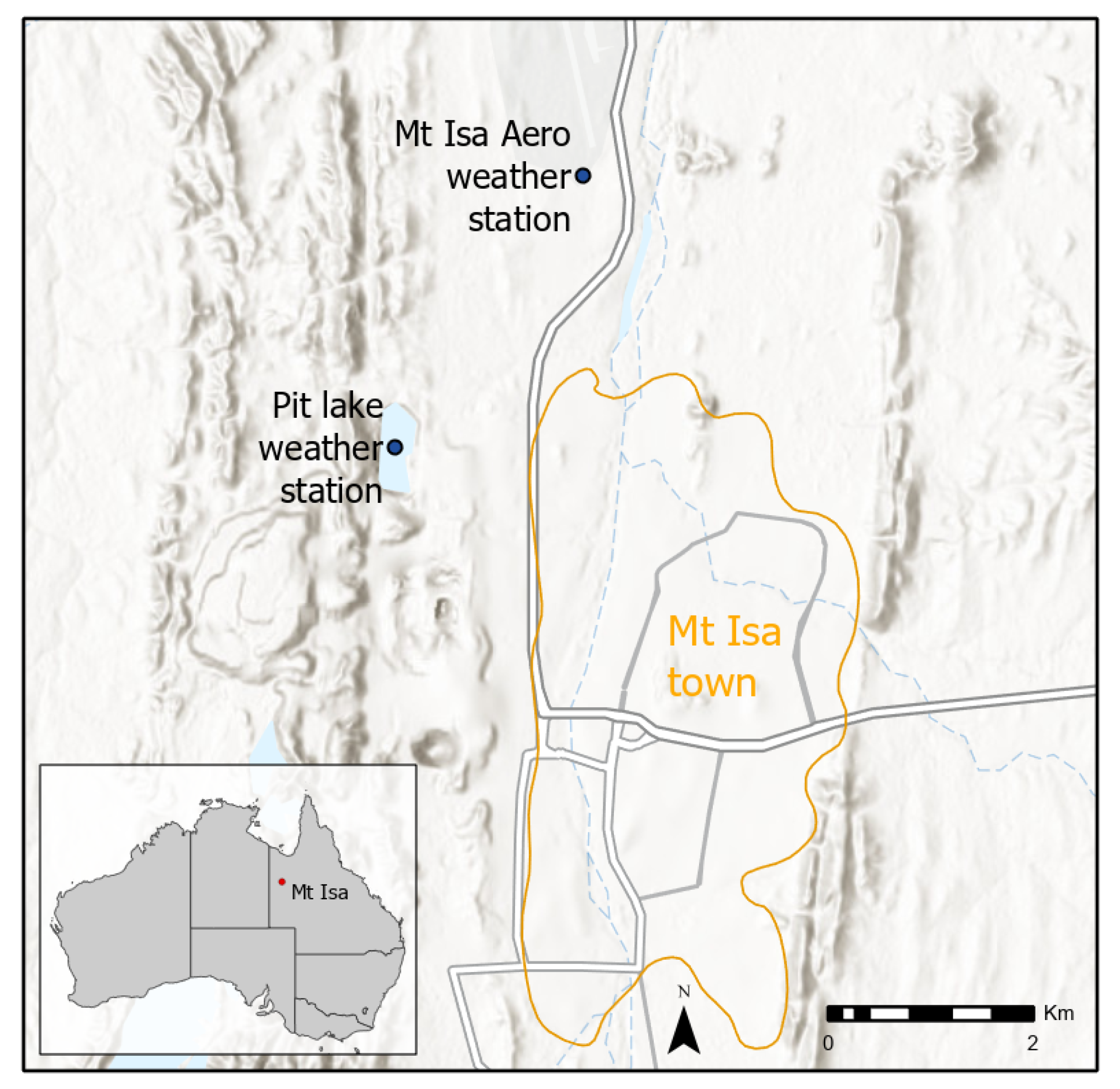
The case study mine pit lake is approximately 1.3 km west of the town of Mount Isa, Queensland, Australia (Figure 1), with the lake bed at approximately 300 m above mean sea level. The climate is classed under the Köppen–Geiger system as semi-arid hot. A long-term weather station exists at Mt Isa airport, approximately 3 km north-east of the pit lake. At this station the mean annual rainfall between 1966 and 2019 was 460 mm, with a maximum of 1092 mm and minimum of 93 mm. Approximately 77% of the total annual rainfall in that period occurred in the four-month wet season, December to March. The average number of wet days (any trace of rain at the weather station rain gauge) ranges from 0.9 in August to 10 in January, averaging 51 per year. The average annual pan evaporation measured at the weather station between 1975 and 2020 was 3061 mm/year with daily evaporation ranging between 5.5 and 11.0 mm/day, with highest evaporation occurring during the wet season. The mine pit is approximately 850 m long and 360 m wide and its base is 50 m below ground level giving an approximate storage capacity of 7 GL. From the crest of the pit to the water level during the evaporation measurement period is 30 m.
Evaporation measurements were obtained from an evaporation pan that was floated in the pit lake between 11 November 2017 and 10 June 2018. Out of the 212 days with evaporation pan data, 2 days were discarded due to high wind and wave action. 60 days were identified as low reliability due to rainfall influencing the pan water level, which could not be accurately corrected for. This resulted in a final set of 150 high quality pan evaporation pan measurement days. A weather buoy was also floated on the pit lake from 11 November 2017 to 1 November 2018. Corrections to the pan evaporation data were made using established methods [5] to account for deviations in the temperature of the water in the pan from that at the lake surface.
2.2. Historical Data Reconstruction
Evaporation data for the period 1974 to 2017 were deterministically modelled based on the in situ measurements. First, following Equation (1), a wind function f(U) is identified using in situ measurements. The in situ floating weather station data and water temperature measurements are used to estimate U, and ea, and the function f(U) was then optimised by least squares regression of the daily Elake/(e*lake -e) values against the measured average daily wind speed. e*lake was calculated using the measured water temperature. The 62 less reliable measurements of evaporation were not used in the fitting, but the model was then employed to in-fill these missing data.
For reconstruction of evaporation over the period 1974–2017, since the in situ floating weather station did not exist prior to 2017, it is necessary to use a modified approach, which relies on data from the nearby long-term weather station. McJannet et al. [5] tested six different models for a mine pit, and concluded that an earlier wind function [19] worked well where in situ data are not used:
where A (m2) is the lake surface area, introduced to allow for water vapour entrainment effects. In this reconstruction, e*lake was calculated using a water temperature equilibrium model [20,21,22]. The equilibrium temperature is the temperature towards which the water temperature is driven by the net heat exchange. The equilibrium temperature model allows an estimate of the temperature of a water body to be derived using standard meteorological measurements. Modelled water temperatures are dependent on the equilibrium temperature, Tw (°C) and a time constant, τ (days). The time constant reflects the time which would be required to reach equilibrium between air and water temperatures if conditions remained stable. Using this method, Tw is calculated as:
where Tw0 (°C) is the water temperature at the previous time step. The full methodology for deriving Te and τ is given in [5].
This approach, here called the “long-term model”, was adopted using weather data from the nearby weather station. It was not re-calibrated to the case study observations for reasons discussed in Section 4. Air temperature, humidity and solar radiation data were extracted from the SILO database for the airport weather station site. SILO is an on-line database that provides historical continuous daily climate data over Australia, including at weather station sites, using spatial interpolation of measurements [23]. After evaluating the long-term model, the daily pit lake evaporation was synthesised for the period 1974–2017 using long-term weather station and SILO data. Gaps in the long-term wind speed data at the weather station were infilled as described in Appendix A.
2.3. Stochastic Models
The Stochastic Climate Library is a library of stochastic models for generating climate data [14] that is commonly used in Australia including for mine pit lake applications [7]. The current study assessed the accuracy of Stochastic Climate Library Version 2.1b in generating annual, monthly and daily stochastic rainfall and evaporation over the 44-year period of reconstructed evaporation data. It is assumed that these 44 years, 1974–2017, represent the climate variability that is relevant for conducting pit lake water balances into the future, and therefore provide a useful test period for the stochastic model under the stationary climate assumption.
The method for the annual, monthly and daily models is summarised here from the Stochastic Climate Library guide [14]. At an annual time step:
where Xt is a 3 × 1 matrix of standardised climate data (annual averages of rainfall, daily maximum air temperature and evaporation) for year t, A and B are 3 × 3 coefficient matrices that preserve the correlations between the three variables, and εt is a random number with zero mean and unit variance presenting the random variability of the three variables. A = M1M0−1 and B = M1M0−1M1T, where M0 and M1 are 3 × 3 matrices that describe the lag zero and lag one cross-correlations between the three modelled variables [14].
The monthly data are generated by a deterministic disaggregation of the stochastically generated annual data. The historical monthly climate data are standardised year by year so that the sum of the monthly climate data in any year equals 1.0. This is carried out by dividing the monthly climate data in each of the 44 years by the corresponding annual climate data, giving 44 sets of monthly-to-annual ratios for the three climate variables. The stochastically modelled annual data for year Y are disaggregated by selecting the monthly-to-annual ratios taken from the historical year Yh that has similar annual climate variable values to year Y, and monthly values in December of year Yh-1 similar to those modelled for year Y-1 (which are known because year Y-1 has already been modelled). To calculate similarity, these two criteria are weighted as explained in the Stochastic Climate Library guide [14] (page 38).
The daily model is a stochastic model, developed independently from the annual and monthly models. Unlike the monthly model, it does not rely on disaggregating annual data but applies a stochastic model to the daily data. First, daily rainfall state is modelled using a Transition Probability Matrix model. This determines the probability of a rain state (four rainfall states are applicable for the case study region: one for zero rainfall and three for non-zero rainfall) as a function of the state on the previous day. A separate Transition Probability Matrix is identified for each of the 12 months. A multi-variate autoregressive model is then identified of the same form used for the annual model. Again, a separate model is identified for each of the 12 months, and a separate model is identified for rainy days and for dry days. The Transition Probability Matrix is applied to generate the rain state time series, then the multi-variate autoregressive model is applied to generate the rainfall, evaporation and maximum temperature data. The climate variables are then scaled up or down for each month using a Thomas–Fiering model [14] (page 39–40), to improve statistical consistency with the historical monthly values (only the non-zero values are scaled in the case of rainfall).
For both the annual and daily models, the climate data are standardised using a Box-Cox transform to achieve an approximately normally distributed, zero-mean and unit variance data set. The model coefficients are identified using least squares theory from the standardised historical data. For the case study, the rainfall and daily maximum temperature measured at the weather station near to the pit lake, and the evaporation reconstructed for the pit, are used for fitting the models. Using the fitted models, 500 replicates of the three variables were generated over a 44-year period at daily, monthly and annual time steps. The models are assessed by judging visually whether statistics calculated from the historical/reconstructed data appear to be sample statistics from the 500 replicates, following common approaches to assessment of stochastic climate models (e.g., [16,17,18]). The statistics used were: mean, standard deviation, skewness coefficient, lag-1 autocorrelation, and cross-correlation between rainfall and evaporation. These statistics are included in the outputs of the Stochastic Climate Library model.
3. Results
3.1. Observed In Situ Weather Data
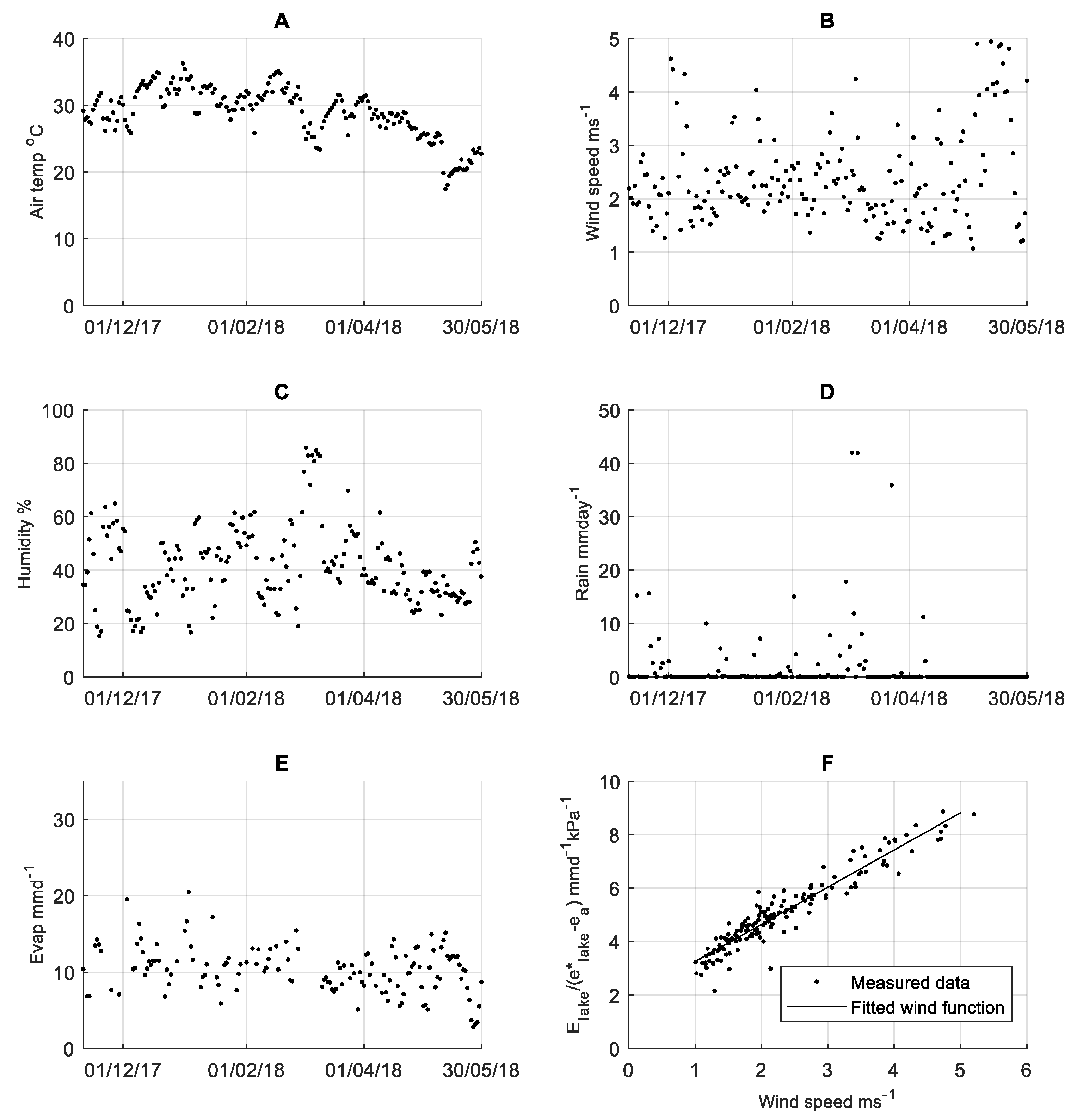
The daily data from the in situ (floating) weather station are shown in Figure 2. Average and maximum wind speeds during the measurement period were 2.4 s−1 and 7.4 ms−1. Total rainfall for the study period was 310 mm and the highest rainfall in one day was 42 mm on 6 March 2018. On average, the surface temperature of the lake was approximately 0.8 °C warmer than that of the pan.
3.2. Identified Wind Function
The values of e*lake and wind speed obtained from the in situ weather station are shown in Figure 2 along with the optimised wind function (Figure 2F):
A total of 92% of the variance of the measured Elake/(e*lake-ea) is explained by the function, with a root mean square error of 0.44 mm day−1kPa−1. Residual analysis did not identify any other relations with climate variables or patterns over time except the slight overestimation Elake/(e*lake-ea) at low wind speeds evident in Figure 2F. This model was used to infill the missing 62 days of evaporation data.
3.3. Constructing Long-Term Evaporation Data
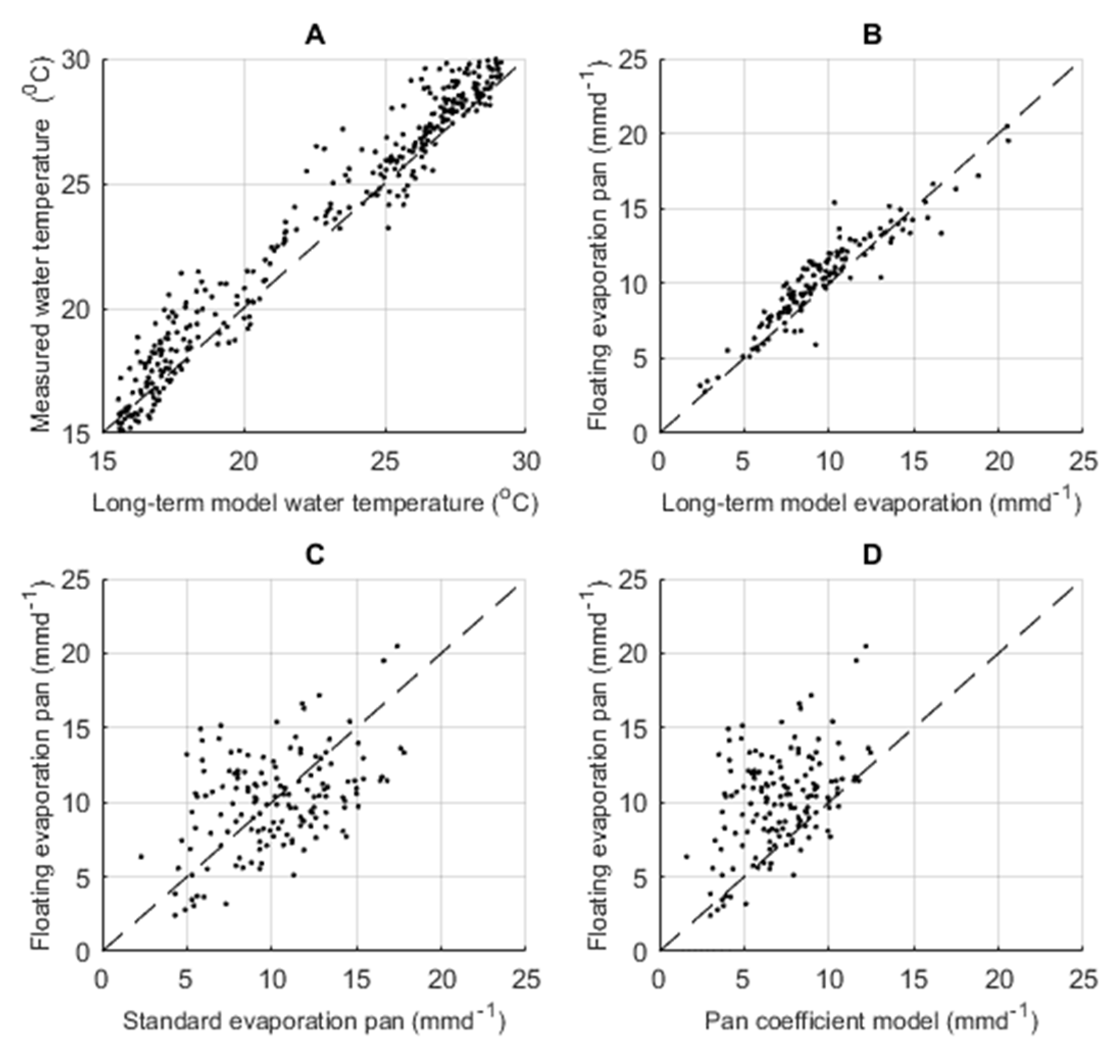
A total of 96% of the observed lake surface temperature variability during the measurement period was explained by the equilibrium temperature model (Figure 3A). This was considered an acceptable result and this model was adopted for reconstructing the long-term daily record for 1974–2017, although with recognised limitations discussed below. The long-term evaporation model, Equation (2), gave the result in Figure 3B. The R2 value is 0.87 and the measured evaporation is underestimated on average by 6.5%. Figure 3C shows that applying the measured pan evaporation from the nearby Mount Isa weather station (location in Figure 1) gives a much higher error variance, while Figure 3D shows that applying a commonly used pan coefficient of 0.7 to that weather station data leads not only to the high variance but to an average bias (underestimate) of 45%.
3.4. Stochastic Model Results
The M0 and M1 matrices obtained from running the annual model are in Table 1. Air temperature is not considered further here but is included in Table 1 for completeness. M0 indicates that rainfall has a strong negative correlation with evaporation. M1 shows that rainfall has a weak positive lag-1 correlation with itself and evaporation has a moderate positive lag-1 correlation with itself. The lag-1 cross-correlations reflect the nature of these other correlations.
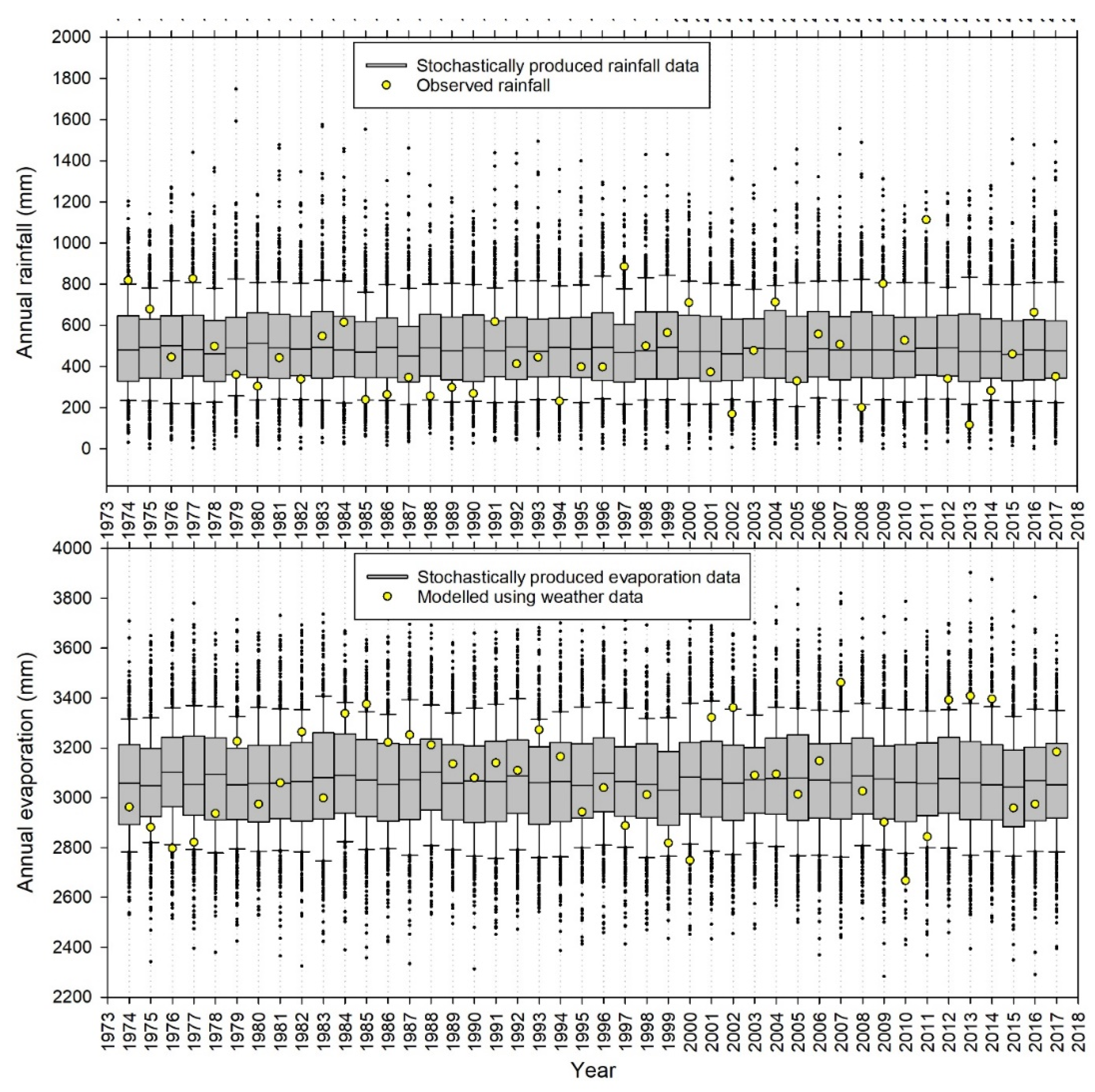
The annual model time-series results are in Figure 4 and selected statistics are in Table 2. Generally, the historical values appear to be samples from the modelled distribution, with the observed statistics close to the median modelled statistics relative to the modelled variance. There are periods, most notably 1985–1990, where the historical record shows persistent dry conditions with high evaporation. Despite representing the historical statistics well (Table 2), the assumed stationarity of the modelled mean leads to limitations in how well the model can capture more complex patterns of persistence. Opportunity to address this is discussed below.
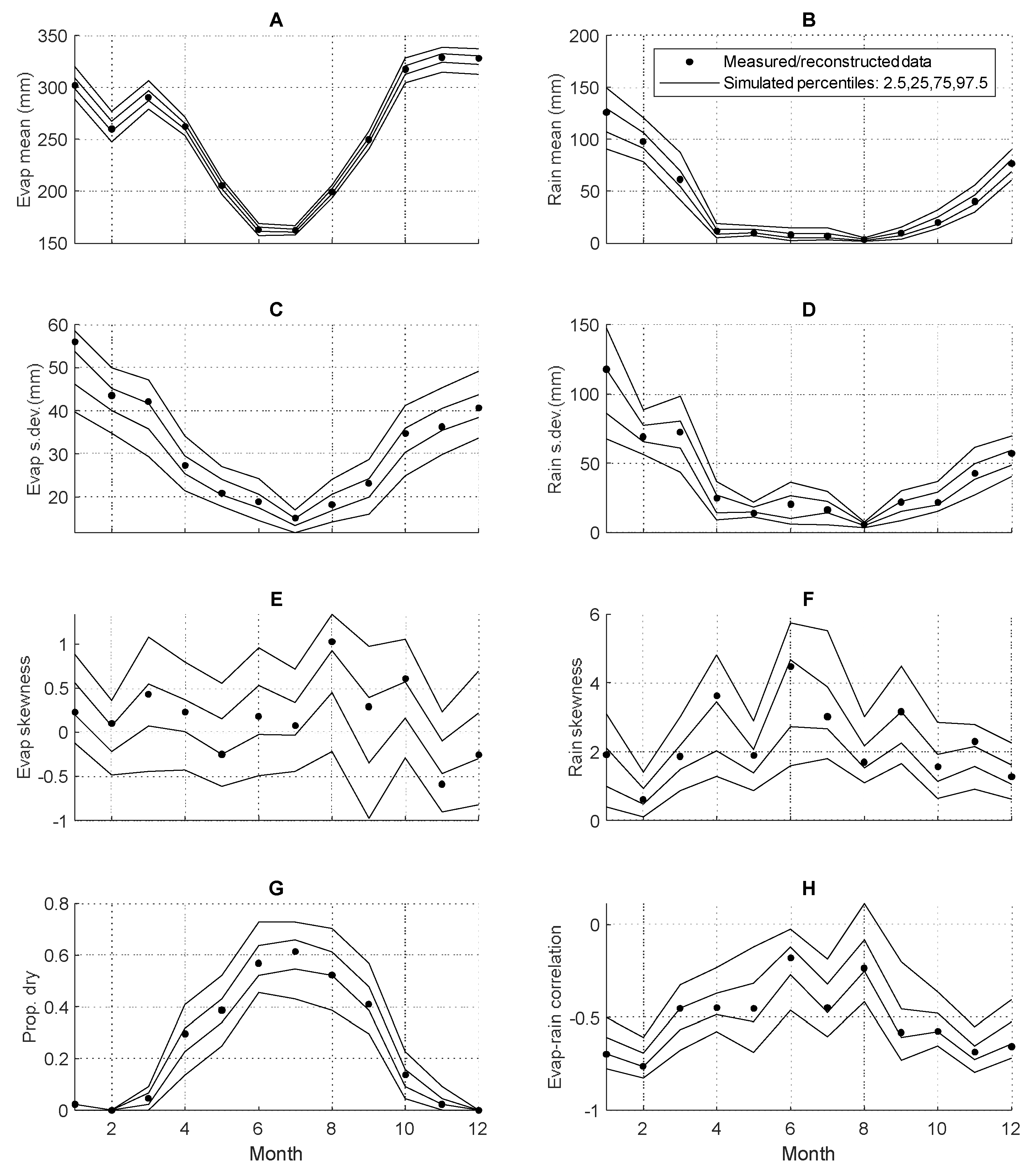
Statistics of the 44 years of output from the monthly stochastic model are shown in Figure 5. If the measured/reconstructed data appear to be a random realisation from the modelled distribution then there is no evidence of bias in the stochastic model. This is the case in Figure 5. This also applies to lag-1 autocorrelations not included in Figure 5. These results would be trivial if the model fitting method guaranteed zero bias in these statistics; however, the data are re-transformed following model fitting and then deterministically disaggregated to monthly values with no subsequent bias removal step, so the result is of interest and indicates the good performance in the fitting period of the monthly stochastic model.
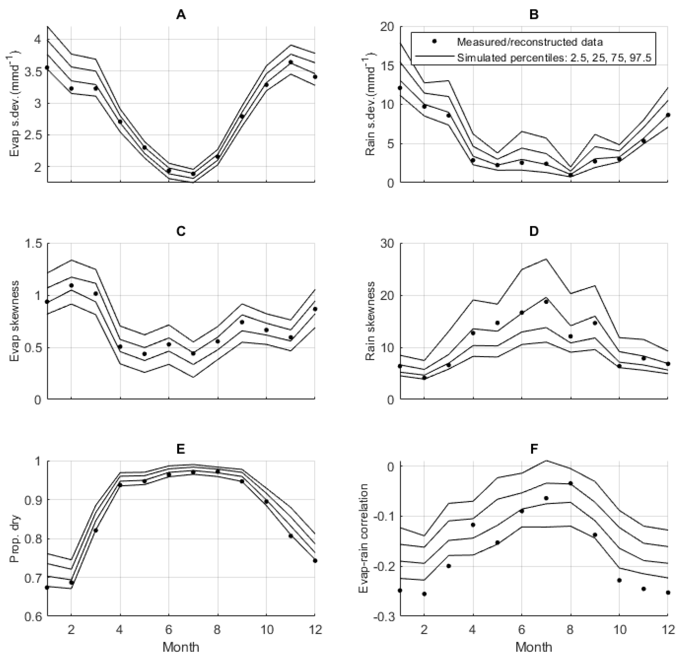
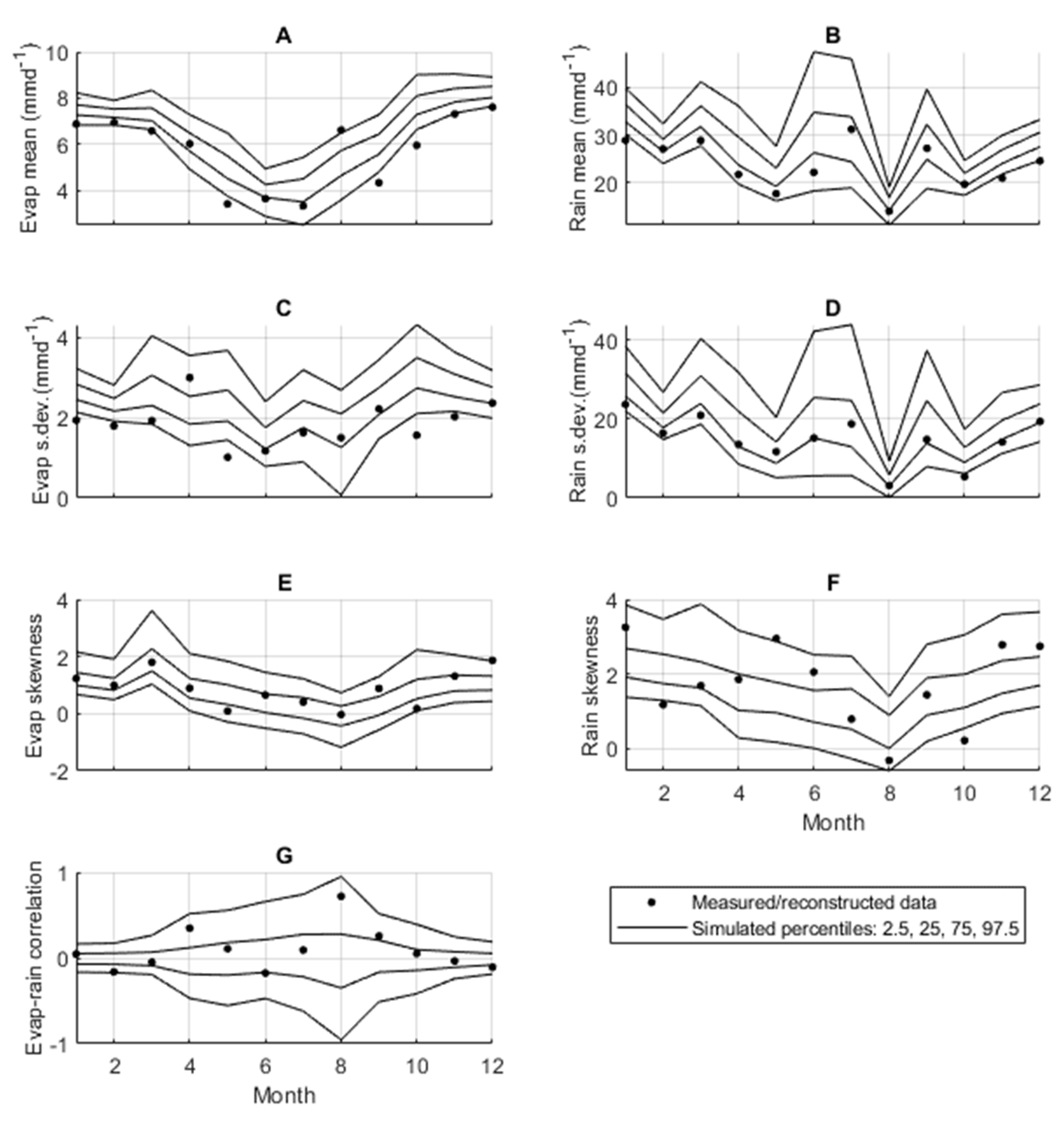
Statistics of the 44 years of output from the daily stochastic model are shown in Figure 6. The statistics in Figure 6 are unconditional on whether the day is dry or wet, while Figure A1 and Figure A2 show the corresponding conditional results. The main result of note here (Figure 6E) is that the model tends to overestimate the number of dry days (in all months except August the measured number of dry days is less than the modelled 25 percentile). Correspondingly, in removing bias in the mean rainfall, it tends to overestimate the volume of rainfall on wet days (Figure A2B). Figure 6F shows that the model consistently underestimates the strength (i.e., the modelled values are not negative enough) of the daily rainfall-evaporation correlation during the wet season, October to March. This corresponds to a tendency of the model to underestimate evaporation on dry days (Figure A1A) and to overestimate evaporation on wet days (Figure A2A). For example, 0.2 mm/day is the mean underestimation for dry days in November and 0.8 mm/day is the mean overestimate for November on wet days. The wet-day modelled rainfall bias is larger in the dry season (for example 2.0 mm/day overestimation in May) but the small number of wet days (5% in May) make this of less concern than the wet season bias.
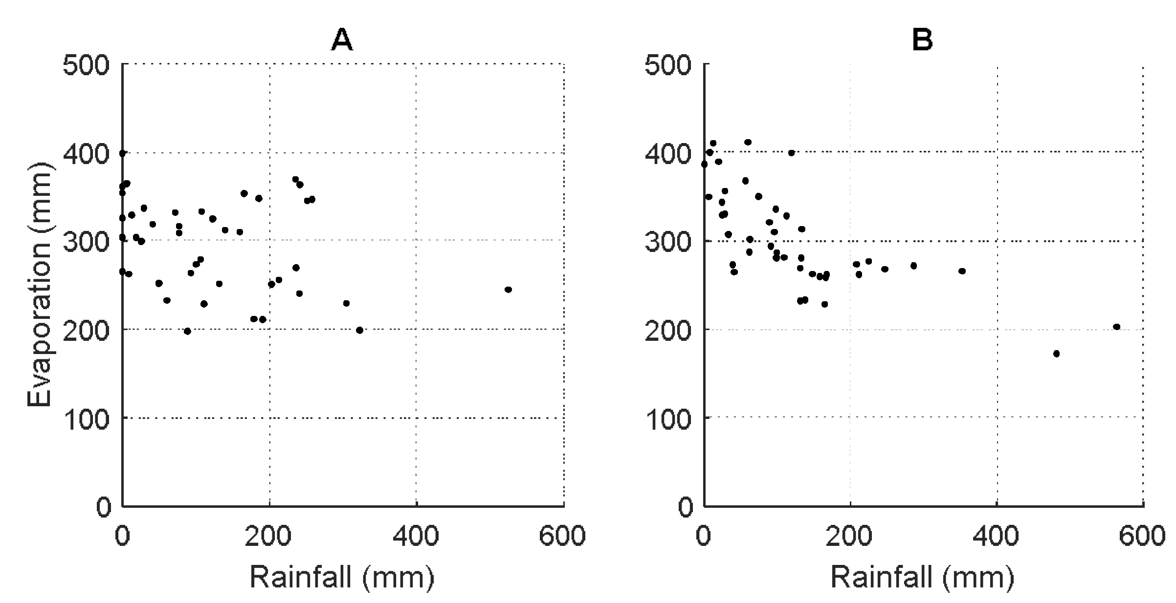
To help understand the nature of the errors in the daily stochastic model of evaporation, a representative model realisation for January (i.e., 44 modelled January results corresponding to the 44 modelled years) is plotted in Figure 7 in comparison to the corresponding observed/reconstructed data. Although produced with the daily model, these data are aggregated to monthly values because this more clearly shows the nature of the errors. Figure 7 illustrates that the observed/reconstructed data show a stronger negative correlation between rainfall and evaporation. Furthermore, the daily stochastic model produces more dry or near-dry months than were observed, with lower evaporation and with higher variance of evaporation.
4. Summary and Discussion
This paper appears to be the first to critically evaluate the joint simulation of rainfall and evaporation using the established and commonly employed Stochastic Climate Library tools [14], and the first to critically evaluate any stochastic climate model for pit lake evaporation. The need for such tools is growing rapidly in Australia due to the large number of mines for which pit closure plans are being developed and for which water balances need to be developed for 100 years or more into the future.
The deterministic model used for reconstructing historical evaporation is considered to accurately represent the measured evaporation on the basis of Figure 3B, which represents the model’s average bias (underestimate) of 6.5%. Although this is small compared to the 45% bias obtained when using the pan coefficient model (Figure 3D), 6.5% cannot be assumed to be insignificant for long-term water balances, and may have arisen due to differences in wind speed between the nearby weather station and pit lake at which evaporation measurements were made. Possible ways to address this include bias adjusting the weather station data so that its mean matches the site data, re-fitting a generalised wind function model [5] using the weather station and measured evaporation data, or simply bias adjusting the modelled evaporation data. Each of these options would require the assumption that the bias was due to the model and not the measurements, and that the adjustment is applicable over the long-term rather than being more specific to the 7-month in situ evaporation measurement period. Therefore, for this paper, the 6.5% underestimation was accepted. In applying the model to reconstruct the historical record, additional uncertainty is introduced due to the infilling and extension of the weather station using a national wind speed data set (method in Appendix A). However, comparison of the evaporation calculated using two sources of wind data, during periods where both sources of wind speed data existed, showed less than 1% difference [24].
A limitation of the measured evaporation data is that it was limited to a 7-month period, 11 November 2017 and 10 June 2018, providing 150 high-quality measurements. Although this 7-month period captured both the wet and dry seasons and a reasonably wide range of weather conditions (see Figure 2), a longer, multi-year period would have captured different and perhaps more extreme weather conditions, potentially affecting the fitted wind function. There is a need to trade-off the cost of maintaining the floating evaporation pan with the value of additional data; nevertheless in future experiments it is recommended that at least 12 months of evaporation measurements are collected following [5].
The fitted wind function implies an overestimation of lake evaporation at low wind speeds (Figure 2F). The absence of lower daily average wind speeds (<1 m/s) limits how well this can be assessed. Hourly analysis was considered, but this resolution is beyond specifications of the instrumentation (12 h is the minimum period over which evaporation can reasonably be measured). Furthermore, the overestimation may be due to reduced reliability of wind data at low speeds. The wind speed sensor used in this study has a ‘startup’ or minimum speed so that wind may not be recorded in a proportion of the 15-s measurement periods in calm days. This could be investigated further using more sensitive wind speed sensors such as the three-dimensional wind sonics used for eddy covariance measurements. Other potential limitations of the wind function model for pit lakes are addressed in a previous pit lake study [5].
The stochastically modelled annual and monthly data are mainly consistent with the historical data. The main caveat on this result is the lack of representation of the persistency of rainfall and evaporation rates between years evident in Figure 4. The annual and monthly stochastic models assume stationary means and are not designed to represent the effects of climate cycles such as that associated with the El Nino Southern Oscillation (ENSO). In order to identify if ENSO has an influence, the rainfall and evaporation residuals were plotted against an ENSO index [25]. The p-value for the linear relation between the index and evaporation was 0.12, and R2 value was 0.005 and for rainfall the p-value was 0.46. Hence, there is some evidence of a potential linear relation between evaporation residual and ENSO; however, if the relation exists, it is weak and it does not explain the magnitude of the residuals observed in Figure 5. Further research could explore the effect of other synoptic climate variables and teleconnection controls that are known to influence weather in this region [26]. Such an extension to the model may also permit the stochastic model to be used for downscaling climate model outputs, or alternative stochastic downscaling frameworks could be employed [27,28].
The stochastic daily model cannot yet be recommended for use in pit lake applications. The daily model overestimates dry day occurrence and wet day rainfall amount, and underestimates the strength of cross-correlation between rainfall and evaporation. These problems are apparent even when the daily outputs are aggregated to monthly data. The mis-representation of dry days may be due to the reliance on the simple Transition Probability Matrix, which only considers the previous day’s state rather than longer-term persistency. The problem with daily occurrence may also be related to the use of the Thomas–Fiering equation and to the assumption of a normal distribution of the monthly variables that is inherent in the method [29]. The Thomas–Fiering equation is used to adjust bias in the daily values according to historical monthly statistics. This is done independently for each of the three climate variables, which may be a cause of the cross-correlation issues. Resolving this requires further research. The daily model is also generating too much variance in the evaporation both in months with low rainfall and high rainfall (Figure 7). This may be associated with the unbounded probability distributions used in the daily evaporation model. The same model [14] puts minimum and maximum bounds on temperature to prevent the model from producing physically unrealistic results. It may be useful to also bound the daily evaporation rate using physically-based models.
The results of the stochastic modelling have implications for long-term pit lake water balance models and decisions regarding synthesis of climate data. The daily stochastic data may be unsuitable due to aforementioned constraints. The monthly stochastic data could be used; however, the rapid rise of lake level due to short duration and high intensity rainfall events would be under-represented. A compromise could be disaggregating the monthly rainfall data but maintaining the monthly evaporation data, since pit lake levels are unlikely to be sensitive to the disaggregation of evaporation. Alternative approaches would ideally be run through the pit lake water balance model to test sensitivity to the necessary assumptions.
From the above discussion, options for improving the accuracy of open water evaporation data used in long-term pit lake water balances include: (1) this and previous studies [5,9] have shown that the adoption of the pan coefficient model is unreliable and should not be used, at least not prior to validation over a wide range of weather conditions, using in situ measurements; (2) the aerodynamic model, Equation (2), is recommended although also would benefit from validation and potential adjustment using in situ measurements, in particular where there is doubt about the applicability of the equilibrium temperature model; (3) stochastic modelling of rainfall and evaporation in environments with irregular rainfall occurrence and extreme variations in both rainfall and evaporation, such as the Mt Isa case study, may be challenging using relatively simple stochastic models such as those in the Stochastic Climate Library; using such models, a monthly time step may be better, followed if necessary by disaggregation of rainfall to a daily time step; (4) in Queensland and other regions subject to strong multi-year cycles in rainfall and evaporation and/or global climate change effects, there is need and opportunity to use stochastic climate models that incorporate non-stationarity [30]; (5) the work undertaken here needs to be complemented by understanding the sensitivity of pit lake water balances to the errors in the evaporation models and other inputs in order to determine priorities for model improvement and data collection [3].
5. Conclusions
This paper addressed the challenge of generating long-term lake evaporation time series for modelling mine pit lake water balances. A data set from a floating evaporation pan and weather station installed at a pit lake at Mount Isa Australia during 2017–2018 provided a rare in situ set of measurements. The modelling included reconstructing a 44-year time series of historical daily evaporation using a deterministic aerodynamic model, and synthesising a 44-year time series of future evaporation using the Stochastic Climate Library [14]. The aerodynamic model underestimated measured evaporation by 6.5% within the measurement period. This error was low compared to alternative simple lake evaporation models, although further work is recommended to determine the reason and significance of the error. Different stochastic models were applied for monthly and daily time steps. Assessment of the monthly model could not detect any biases in the monthly statistics including the cross-correlation between evaporation and rainfall. However, the model could not (and was not designed to) represent the observed multi-year anomalies in rainfall and evaporation, hence there are applicability questions for cases where multi-year persistency may be important, for which more sophisticated stochastic modelling tools may be better. The daily stochastic model results showed bias in various rainfall and evaporation statistics, which may be related to the difficulty in modelling transitions between wet and dry days in the semi-arid climate of the case study. Caution is required in using the daily stochastic model in this and similar climates.
Author Contributions
Conceptualization, K.M., N.M. and D.M.; methodology, K.M., N.M. and D.M.; formal analysis, K.M.; writing—original draft preparation, K.M.; writing—review and editing, K.M., N.M. and D.M. All authors have read and agreed to the published version of the manuscript.
Funding
This research was funded by Glencore, Mount Isa Mines Ltd.
Data Availability Statement
Requests to access the data should be sent to the corresponding author.
Acknowledgments
The case study site is on the traditional lands of the Kalkadoon and Indjilandji people. The authors acknowledge the Traditional Owners and their custodianship of the lands, and pay our respects to their Ancestors and their descendants. The measured evaporation and in situ climate data were provided by Glencore and the modelling research was primarily funded by Glencore. The authors gratefully acknowledge Glencore’s support of hydrological research. Thank you to Pascal Bolz of The University of Queensland for production of Figure 1.
Conflicts of Interest
The authors declare no conflict of interest.
Appendix A. Infilling of Historical Wind Speed Data
The procedure for infilling historical wind speed data from the BILO database (McVicar et al. 2008) was: (1) BOM wind speed and Buoy wind speed were compared over the 11 November 2017 to 01 November 2018 to determine a conversion equation and the correction equation is then applied to the entire BOM wind speed data set; (2) Wind speed values in the BOM data set <0.5 m/s were ignored, as on these days readings were typically only made twice a day and are not representative of an average; (3) 20 years of scaled BOM data were compared to the BILO data to develop an equation to scale BILO data to represent Buoy wind speed; (4) The gaps in the scaled BOM data were filled with the scaled BILO data to produce a final wind data set.
Appendix B. Performance of Daily Stochastic Model Conditional on whether the Day Is Wet or Dry
Figure A1.
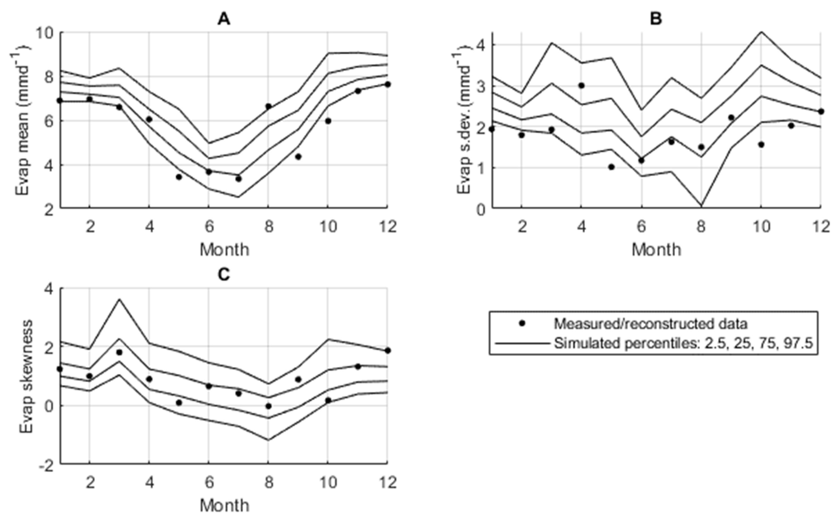
Stochastic model performance for evaporation on dry days: (A) Evaporation mean; (B) Evaporation standard deviation; (C) Evaporation skewness coefficient.
Figure A1.
Stochastic model performance for evaporation on dry days: (A) Evaporation mean; (B) Evaporation standard deviation; (C) Evaporation skewness coefficient.

Figure A2.
Stochastic model performance for evaporation and rainfall on wet days (rainfall > 10 mm/day): (A) Evaporation mean; (B) Rainfall mean; (C) Evaporation standard deviation; (D) Rainfall standard deviation; (E) Evaporation skewness coefficient; (F) Rainfall skewness coefficient; (G) Evaporation–rainfall correlation coefficient.

References
- McCullough, C.D.; Lund, M.A. Opportunities for sustainable mining pit lakes in Australia. Mine Water Environ. 2006, 25, 220–226. [Google Scholar] [CrossRef]
- McCullough, C.D.; Marchand, G.; Unseld, J. Mine closure of pit lakes as terminal sinks: Best available practice when options are limited? Mine Water Environ. 2013, 32, 302–313. [Google Scholar] [CrossRef] [Green Version]
- Cook, P.G.; Black, S.; Cote, C.; Kahe, M.S.; Linge, K.; Oldham, C.; Ordens, C.; McIntyre, N.; Simmons, C.; Wallis, I. Hydrological and Geochemical Processes and Closure Options for Below Water Table Open Pit Mines; CRC TiME Limited: Perth, Australia, 2021. [Google Scholar]
- Paulsson, O.; Widerlund, A. Modelled impact of climate change scenarios on hydrodynamics and water quality of the Rävlidmyran pit lake, northern Sweden. Appl. Geochem. 2022, 139, 105235. [Google Scholar] [CrossRef]
- McJannet, D.; Hawdon, A.; Van Niel, T.; Boadle, D.; Baker, B.; Trefry, M.; Rea, I. Measurements of evaporation from a mine void lake and testing of modelling approaches. J. Hydrol. 2017, 555, 631–647. [Google Scholar] [CrossRef]
- McJannet, D.; Hawdon, A.; Baker, B.; Ahwang, K.; Gallant, J.; Henderson, S.; Hocking, A. Evaporation from coal mine pit lakes: Measurements and modelling. In Mine Closure 2019: Proceedings of the 13th International Conference on Mine Closure, Eds. Fourie, A.B. and Tibbett, M., Australian Centre for Geomechanics, Perth, Australia; Australian Centre for Geomechanics: Crawley, Australia, 2019; pp. 1391–1404. [Google Scholar] [CrossRef] [Green Version]
- Zhan, W.; Nathan, R.; Buckley, S.; Hocking, A. Climate Change Adaptation in BHP’s Queensland Mine Water Planning and Hydrologic Designs. In Proc. Of IMWA; Pope, J., Wolkersdorfer, C., Weber, A., Sartz, L., Wolkersdorfer, K., Eds. 2020. Available online: https://www.imwa.info/docs/imwa_2020/IMWA2020_Zhan_231.pdf (accessed on 24 November 2022).
- Hounam, C.E. Comparison between Pan and Lake Evaporation; Technical Note No. 126; World Meteorological Organisa-tion: Geneva, Switzerland, 1973. [Google Scholar]
- Finch, J.; Calver, A. Methods for the Quantification of Evaporation from Lakes; Centre for Ecology and Hydrology: Wallingford, UK, 2008. [Google Scholar]
- McJannet, D.L.; Cook, F.J.; Burn, S. Comparison of techniques for estimating evaporation from an irrigation water storage. Water Resour. Res. 2013, 49, 1415–1428. [Google Scholar] [CrossRef]
- Tuheteru, E.J.; Gautama, R.S.; Kusuma, G.J.; Kuntoro, A.A.; Pranoto, K.; Palinggi, Y. Water balance of pit lake development in the equatorial region. Water 2021, 13, 3106. [Google Scholar] [CrossRef]
- McMahon, T.A.; Peel, M.C.; Lowe, L.; Srikanthan, R.; Mcvicar, T.R. Estimating actual, potential, reference crop and pan evaporation using standard meteorological data: A pragmatic synthesis. Hydrol. Earth Syst. Sci. 2013, 17, 1331–1363. [Google Scholar] [CrossRef] [Green Version]
- La Fuente, S.; Jennings, E.; Gal, G.; Kirillin, G.; Shatwell, T.; Ladwig, R.; Moore, T.; Couture, R.-M.; Côté, M.; Vinnå, C.L.R.; et al. Multi-model projections of future evaporation in a sub-tropical lake. J. Hydrol. 2022, 615 Pt A, 128729. [Google Scholar] [CrossRef]
- Srikanthan, S.; Chiew, F.; Frost, A. Stochastic Climate Library User Guide, v2.1b; CRC for Catchment Hydrology: Canberra, Australia, 2007. [Google Scholar]
- Peleg, N.; Fatichi, S.; Paschalis, A.; Molnar, P.; Burlando, P. An advanced stochastic weather generator for simulating 2-D high-resolution climate variables. J. Adv. Model. Earth Syst. 2017, 9, 1595–1627. [Google Scholar] [CrossRef]
- Chandler, R.E. Multisite, multivariate weather generation based on generalised linear models. Environ. Model. Softw. 2020, 134, 104867. [Google Scholar] [CrossRef]
- Duan, J.; McIntyre, N.; Onof, C. A regional rainfall model for drought risk assessment in south-east UK. Proc. Inst. Civil Eng. Water Manag. 2013, 166, 519–535. [Google Scholar] [CrossRef] [Green Version]
- Kenabatho, P.; McIntyre, N.; Chandler, R.; Wheater, H. Stochastic simulation of rainfall in the semi-arid Limpopo basin. Int. J. Climatol. 2012 32, 1113–1127. [CrossRef]
- McJannet, D.L.; Webster, I.T.; Cook, F.J. An area-dependent wind function for estimating open water evapo-ration using land-based meteorological data. Environ. Model. Softw. 2012, 31, 76–83. [Google Scholar] [CrossRef]
- De Bruin, H.A.R. Temperature and energy balance of a water reservoir determined from standard weather data of a land station. J. Hydrol. 1982 59, 261–274. [CrossRef]
- Edinger, J.E.; Duttweiler, D.W.; Geyer, J.C. The response of water temperature to meteorological conditions. Water Resour. Res. 1968, 4, 1137–1143. [Google Scholar] [CrossRef]
- Keijman, J.Q. The estimation of the energy balance of a lake from simple weather data. Bound. Layer Meteorol. 1974, 7, 399–407. [Google Scholar] [CrossRef]
- Jeffrey, S.J.; Carter, J.O.; Moodie, K.B.; Beswick, A.R. Using spatial interpolation to construct a comprehensive archive of Australian climate data. Environ. Modell. Softw. 2001, 16, 309–330. [Google Scholar] [CrossRef]
- Mandaran, K.J. Modelling Evaporation from a Mine Pit Lake. Master of Philosophy Thesis, The University of Queensland, Brisbane, Australia, 2021. [Google Scholar]
- Smith, C.A.; Sardeshmukh, P. The effect of ENSO on the intraseasonal variance of surface temperature in winter. Int. J. Climatol. 2000, 20, 1543–1557. [Google Scholar] [CrossRef]
- Klingaman, N.P.; Woolnough, S.J.; Syktus, J. On the drivers of inter-annual and decadal rainfall variability in Queensland, Australia. Int. J. Climatol. 2013, 33, 2413–2430. [Google Scholar] [CrossRef]
- Mehrotra, R.; Sharma, A. Development and Application of a Multisite Rainfall Stochastic Downscaling Framework for Climate Change Impact Assessment. Water Resour. Res. 2010, 46, W07526. [Google Scholar] [CrossRef]
- Chandler, R.E. On the use of generalized linear models for interpreting climate variability. Environmetrics 2005, 16, 699–715. [Google Scholar] [CrossRef]
- Harms, A.A.; Campbell, T.H. An extension tothe Thomas-Fiering Model for the sequentialgeneration of streamflow. Water Resour. Res. 1967, 3, 653–661. [Google Scholar] [CrossRef]
- Kiem, A.S.; Kuczera, G.; Kozarovski, P.; Zhang, L.; Willgoose, G. Stochastic generation of future hydroclimate using temperature as a climate change covariate. Water Resour. Res. 2021, 57, 2020WR027331 doiorg/101029/2020WR027331. [Google Scholar] [CrossRef]
Figure 1.
Pit lake and regional weather station locations.

Figure 2.
Data measured at the pit lake floating weather station: (A) average daily temperature; (B) wind speed; (C) relative humidity; (D) rainfall; (E) evaporation; (F) Elake/(e*lake-ea) against wind speed.
Figure 2.
Data measured at the pit lake floating weather station: (A) average daily temperature; (B) wind speed; (C) relative humidity; (D) rainfall; (E) evaporation; (F) Elake/(e*lake-ea) against wind speed.

Figure 3.
Scatter plots of: (A) surface water temperature modelled using the equilibrium model vs. measured surface water temperature; (B) evaporation using the long-term model vs. evaporation measured using the floating evaporation pan; (C) evaporation measured at the Mount Isa weather station vs. evaporation measured using the floating evaporation pan; (D) applying a pan coefficient of 0.7 to evaporation measured at the Mount Isa weather station vs. evaporation measured using the floating evaporation pan.

Figure 4.
Comparison of reconstructed evaporation and measured rainfall with results of annual stochastic simulations The box plots show 10th, 25th, 50th, 75th and 90th percentiles of model realisations with outliers shown as dots.
Figure 4.
Comparison of reconstructed evaporation and measured rainfall with results of annual stochastic simulations The box plots show 10th, 25th, 50th, 75th and 90th percentiles of model realisations with outliers shown as dots.

Figure 5.
Comparison of reconstructed evaporation and measured rainfall statistics with results of monthly stochastic simulations (Month 1 = January): (A) evaporation mean; (B) rainfall mean; (C) evaporation standard deviation; (D) rainfall standard deviation; (E) evaporation skewness coefficient; (F) rainfall skewness coefficient; (G) proportion of months that are dry; (H) evaporation–rainfall correlation coefficient.

Figure 6.
Comparison of reconstructed evaporation and measured rainfall statistics with results of daily stochastic simulations for each month (Month 1 = January): (A) evaporation standard deviation; (B) rainfall standard deviation; (C) evaporation skewness coefficient; (D) rainfall skewness coefficient; (E) proportion of days that are dry; (F) evaporation–rainfall correlation coefficient. Plots of mean values not shown because they are identical to those in Figure 5.

Figure 7.
Relationship between evaporation and rainfall: (A) a representative sample realisation from the daily stochastic model (correlation coefficient = −0.31); (B) reconstructed evaporation and measured rainfall data (correlation coefficient = −0.70).
Figure 7.
Relationship between evaporation and rainfall: (A) a representative sample realisation from the daily stochastic model (correlation coefficient = −0.31); (B) reconstructed evaporation and measured rainfall data (correlation coefficient = −0.70).


Table 1.
Annual stochastic climate model correlation matrices.
| Matrix M0 | |||
|---|---|---|---|
| Variable | Rainfall | Evaporation | Max Temperature |
| Rainfall | 1.000 | −0.771 | −0.679 |
| Evaporation | −0.771 | 1.000 | 0.778 |
| Max Temperature | −0.679 | 0.778 | 1.000 |
| Matrix M1 | |||
| Variable | Rainfall | Evaporation | Max Temperature |
| Rainfall | 0.079 | −0.033 | −0.069 |
| Evaporation | −0.403 | 0.311 | 0.277 |
| Max Temperature | −0.228 | 0.215 | 0.383 |
Table 2.
Annual stochastic model results: comparison of statistics of modelled and measured rainfall and evaporation.
Table 2.
Annual stochastic model results: comparison of statistics of modelled and measured rainfall and evaporation.
| Simulated Percentiles using 500 Replicates | |||||||
|---|---|---|---|---|---|---|---|
| Value Observed during 1974–2017 | 10% | 25% | 50% | 75% | 90% | ||
| Rainfall | Mean (mm) | 467 | 403 | 441 | 465 | 490 | 534 |
| Standard deviation (mm) | 212 | 161 | 191 | 209 | 228 | 268 | |
| Skewness coefficient | 0.89 | 0.07 | 0.48 | 0.72 | 1.01 | 1.81 | |
| Evaporation | Mean | 3056 | 2961 | 3027 | 3061 | 3091 | 3146 |
| Standard deviation | 232 | 179 | 210 | 226 | 245 | 278 | |
| Skewness coefficient | −0.141 | −0.758 | −0.331 | −0.086 | 0.119 | 0.532 | |
| Rainfall-evaporation | Cross-correlation | −0.681 | −0.807 | −0.718 | −0.665 | −0.611 | −0.498 |
Publisher’s Note: MDPI stays neutral with regard to jurisdictional claims in published maps and institutional affiliations. |
© 2022 by the authors. Licensee MDPI, Basel, Switzerland. This article is an open access article distributed under the terms and conditions of the Creative Commons Attribution (CC BY) license (https://creativecommons.org/licenses/by/4.0/).
Share and Cite
MDPI and ACS Style
Mandaran, K.; McIntyre, N.; McJannet, D. Deterministic and Stochastic Generation of Evaporation Data for Long-Term Mine Pit Lake Water Balance Modelling. Water 2022, 14, 4123. https://doi.org/10.3390/w14244123
AMA Style
Mandaran K, McIntyre N, McJannet D. Deterministic and Stochastic Generation of Evaporation Data for Long-Term Mine Pit Lake Water Balance Modelling. Water. 2022; 14(24):4123. https://doi.org/10.3390/w14244123
Chicago/Turabian StyleMandaran, Kristian, Neil McIntyre, and David McJannet. 2022. "Deterministic and Stochastic Generation of Evaporation Data for Long-Term Mine Pit Lake Water Balance Modelling" Water 14, no. 24: 4123. https://doi.org/10.3390/w14244123
Note that from the first issue of 2016, this journal uses article numbers instead of page numbers. See further details here.