
Long-Term Temporal Flood Predictions Made Using Convolutional Neural Networks
by
 ,
,
Hau-Wei Wang
1,*,
Gwo-Fong Lin
2,
Chih-Tsung Hsu
3,
Shiang-Jen Wu
4 and
Samkele Sikhulile Tfwala
5 1
National Center for High-Performance Computing, National Applied Research Laboratories, Taichung City 40763, Taiwan
2
Department of Civil Engineering, National Taiwan University, Taipei City 10617, Taiwan
3
National Center for High-Performance Computing, National Applied Research Laboratories, Hsinchu City 30076, Taiwan
4
Department of Civil and Disaster Prevention Engineering, National United University, Miao-Li County 36063, Taiwan
5
Department of Geography, Environmental Science and Planning, University of Eswatini, Kwaluseni M201, Eswatini
*
Author to whom correspondence should be addressed.
Water 2022, 14(24), 4134; https://doi.org/10.3390/w14244134
Submission received: 8 November 2022
/
Revised: 9 December 2022
/
Accepted: 9 December 2022
/
Published: 19 December 2022
(This article belongs to the Special Issue Advances in Flood Frequency and Inundation Modeling: Application of Statistical, Hydrodynamic, Remote Sensing, and Machine Learning Tools)
Abstract
:This study proposes a method for predicting the long-term temporal two-dimensional range and depth of flooding in all grid points by using a convolutional neural network (CNN). The deep learning model was trained using a large rainfall dataset obtained from actual flooding events, and the corresponding raster flood data computed using a physical model. Various rainfall distributions (at different times or over different accumulation periods), the mesh of the simulated area, and the topography of the simulated area were considered when evaluating the performance of two CNNs: a simple CNN and Inception CNN. Neither CNN architecture could converge when the coordinate information was not included in the input data. Adding terrain elevation information to the rainfall data already containing coordinates increased the accuracy of flood prediction. Our findings indicated that in the proposed method, real-time flooding observation data are not required for corrections, and we concluded that the method can be used for long-term flood forecasting. Our model can accurately pinpoint when the water level changes from rising to falling. Once meteorological forecasted rainfall data are obtained, a corresponding long-term forecast of the two-dimensional flooding range and depth can be obtained within seconds.
1. Introduction
Several methods and tools have been successfully employed in studies investigating flooding, such as unmanned aerial vehicles (UAVs), physical models, and artificial intelligence (AI). UAVs have primarily been used in disaster investigation, assessment, and risk management post a flood event [1,2] and in model validation [3]. Salmoral et al. [4] established guidelines for UAV-based emergency response to flooding. Many physical models have been developed; Teng et al. [5] reviewed several physical models for determining flood inundation, including shallow water wave equations [6,7], two-dimensional dynamic wave equations [8,9], one-dimensional and two-dimensional model coupling simulation of urban flooding [10], and a cellular model [11]. In addition, several commercial models exist, including SOBEK, DELFT3D, 3Di, FLOW-3D, Riverflow2D, MIKE Flood etc. Considerable computing resources are often required to obtain accurate results with both high temporal and spatial resolution. This high resource requirement results in a backlog during the response to a disaster. For hydraulics experts, achieving a trade-off between numerical methods, calculation scales, and calculation efficiency when performing calculations as a reference for flood response is challenging. To solve this problem, many scholars have applied machine learning (ML) methods. Using AI to consider all physical variables is impractical; instead, AI can be employed to select the factors that most strongly affect flooding. The application of ML in flooding disaster prevention mostly involves the solution of one-dimensional river flow problems [12,13] and water level prediction problems [14]; promising results have been obtained for real-time nowcasting predictions.
Flood predictions are often made by making maps of flooding potential, using a physical model, or AI method to predict flooding areas with observational data. ML methods have been applied to many geological parameters to construct two-dimensional maps of flooding potential [15,16,17]. Zhao et al. [18] proposed a convolutional neural network (CNN)-based approach to assess flood susceptibility in an urban catchment. Nine explanatory factors covering precipitation, topographical, and anthropogenic aspects were selected, and two CNNs, namely the simple CNN (SCNN) and LeNet-5, were used to identify the relationship between the explanatory factors and the 2004–2014 flood inventory for the Dahonmen catchment in Beijing, China.
Numerous scholars have attempted to predict the maximum flooding depth during a flood event. Based on the cellular automata approach, Jamali et al. [19] developed a fast flood inundation model for predicting the maximum inundation depth during a single rainfall event simulation lasting from seconds to a few minutes. Guo et al. [20] proposed a CNN method for predicting the maximum water depth; an image-to-image translation problem is considered in which water depth rasters are generated using information learned from data rather than simulations. Their training data included flood simulation data from three catchments and 18 hyetographs. Berkhahn et al. [21] proposed an artificial neural network–based model for predicting the maximum water levels during a flash flooding event. The model was trained with precipitation rates as the input and two-dimensional distributed maximum water levels as the output. The maximum water levels employed for the training were generated using a detailed one–two-dimensional dual drainage model. Scholars have recently focused on predicting temporal variation in the two-dimensional spatial extent of flooding. Chang et al. [22] used SOM classified area flooding data, combined with the R-NARX model and observation data in the past few hours, to predict the area’s total flooded volume in the next 1–3 h.
Various ML methods have been used in the field of hydrology, such as support vector regression, gated recurrent units, recurrent neural networks (RNNs), and long short-term memory (LSTM). Of these methods, RNNs and LSTM have strong backward memory functions. However, water hydrology issues are not as logical and context related as words. They are often highly unpredictable due to changes in rainfall or the environment, and real-time observation data are required to correct trends or reflect the magnitude of effects. Usually, the prediction result is an extension of physical data (and thus generally inaccurate when the rainfall or water level changes suddenly). Therefore, immediateness cannot be achieved when making flood predictions, or these predictions are limited to only a short period.
This study used data produced by physical models as input conditions; these data reflected extreme climate conditions. The quality and rationality of the data affected the training results. If more accurate physical model results are obtained in the future, they can be used as training data to increase the accuracy of the present AI training results. Therefore, whether the original data employed in this study achieved perfect accuracy was not a priority in this study.
Flooding is affected by rainfall intensity, duration, and accumulated rainfall in different periods. By inputting the rainfall distribution at various times into different image channels of a CNN, the CNN can learn to map the range and depth of flooding; alternatively, if the spatial accumulated rainfall distribution in different periods is input, more accurate CNN-learned results can be obtained. For CNN training, the input image is generally already a two-dimensional array of data, with coordinate information included. A CNN should be able to learn the position and depth of flooding. In our construction of an AI flooding-prediction model, we examined if adding spatial information was necessary, and the related effects. This study compared the effect of adding elevation information to the sensitivity of learning by the CNN.
The rest of the paper is structured as follows: Section 2 provides a brief description of the data used in this study and how the data were selected. In Section 3, the CNN architectures used in this study are introduced, as well as the method used to compare the output results of the two architectures, including the total flooding volume comparison, and the method used to compare the difference between two images. Section 4 provides a discussion of the convergence of the two CNN architectures when various combinations of rainfall data types and grids (excluding XYZ coordinates, including XY coordinates, and including terrain elevation) were used. The convergence of the training process indirectly reflected the success or failure of the established model. In Section 5, the predictions made by the model were compared with the results of the physical model, including comparisons of the total flooding volume, similarity, and location of the maximum flooding depth. A complete rainfall event scenario was selected to illustrate how flooding would vary in a single location with time, and under the two-dimensional method applied.
2. Study Area and Data Description
Since not many complete sets of two-dimensional flooding data are available, many two-dimensional simulation datasets were used for training. The historical rainfall data and Monte Carlo methods were used to generate spatial rainfall data. The SOBEK model was used to simulate the flooding range and depth for training. A flood-prone area in northern Taiwan, namely the Dongmen drainage, was selected as the area of interest in this study.
2.1. Study Area
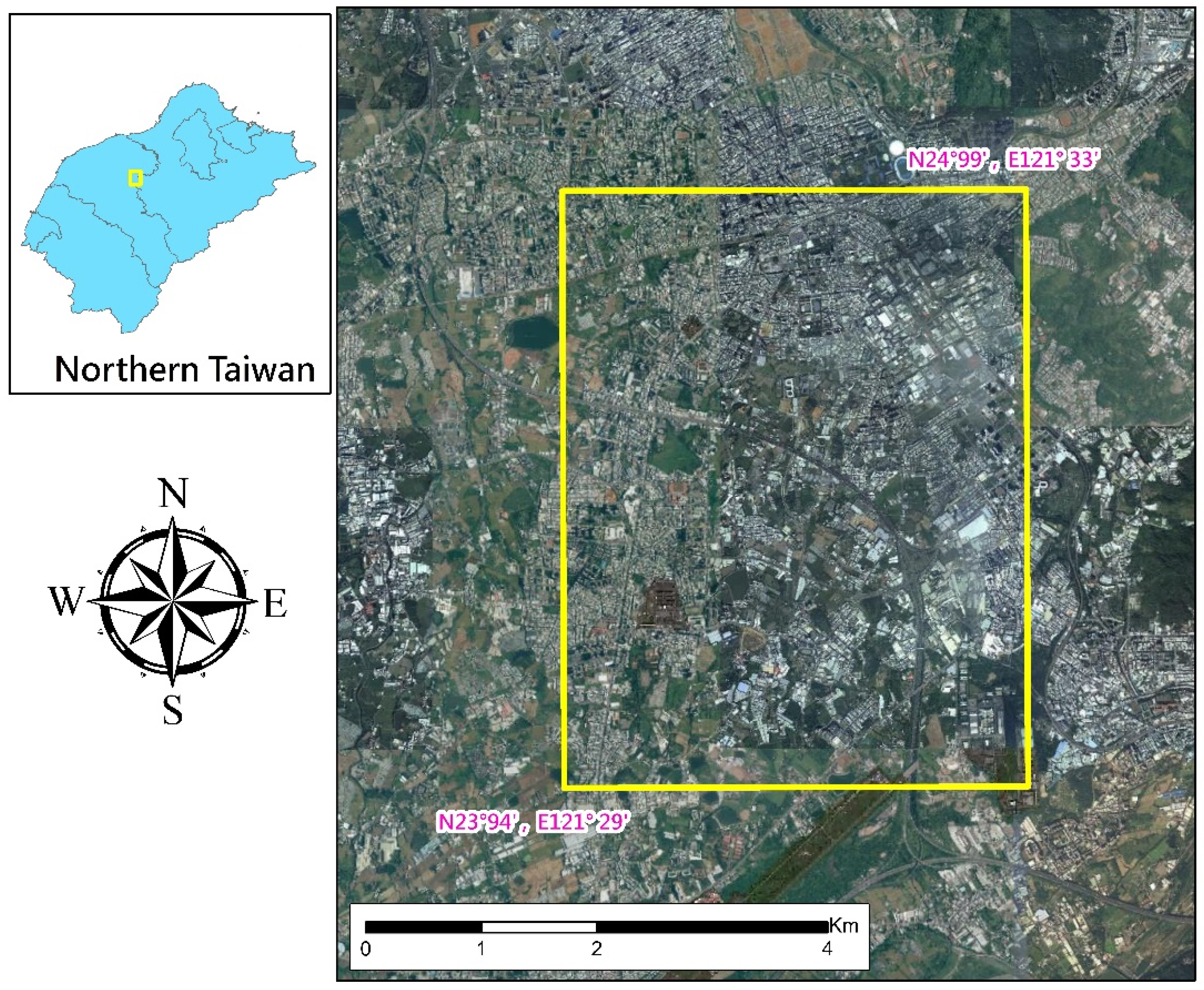
The study area was the Dongmen drainage in northern Taiwan, with an area of approximately 22.22 km2, as illustrated in Figure 1. The drainage was designed under the assumption of a 10-year flood recurrence interval. No bank revetment is present in some river sections, and box culverts are insufficient in the area prone to flooding. Blocking weirs have been erected in some river sections, which has raised the water level and affected upstream drainage. All these factors contribute to flooding in the Dongmen drainage.
2.2. Rainfall Data
The base data employed in this study were data on 21 historical events from 2005 to 2017 (Table 1). These data were obtained using Taiwan’s Quantitative Precipitation Estimation and Segregation Using Multiple Sensors system and were provided by the Central Weather Bureau of Taiwan. Considering the variability in the spatiotemporal properties of rainfall, including its duration, the total precipitation, and the rainfall pattern, this study employed the single-station sequential rainfall characteristics simulation mechanism developed by Wu et al. [23], and the method of stochastic modeling of gridded short-term rainstorms developed by Wu et al. [24] to produce numerous rainfall events. Climate change will affect flooding conditions in the future. Two and three times the mean rainfall and standard deviation factors of the base data were considered. By applying these statistical properties of precipitation, we produced data on 6000 events, with each event containing 25 to 75 h of spatial rainfall (Table 2).
2.3. Flooding Data
The physical flooding model used for producing the flooding data (the SOBEK model) considers the influence of the relationship between the upstream and downstream of the one-dimensional river system and the cross-basin flow of the two-dimensional overland flow; a two-dimensional flooding model of the entire Dongmen drainage was constructed for simulations. A 20-m digital elevation model of the main study area was also employed. The total number of grid squares in the 20-m simulation area was 360 × 201 = 72,360. The 6000 produced rainfall events were used in the simulations to obtain 6000 sets of potential flood events. For each event, 25 to 75 h of flooding was simulated, with the time resolution being 1 h; in total, 218,850 h of spatial flooding data were obtained. The different event data represent the results of simulations for various possible rainfall patterns and the corresponding flooding. Calculating a flooding result for each hour of rainfall took approximately 3 min. More computation time was needed when the simulation area was more extensive, or the grid resolution was finer. The data generated by the physical flooding model, whether used to train the AI flooding model or the flooding data used to compare with the AI flooding model, we refer to as the “actual value” in all the following content.
2.4. Strategy of Data Selection from the Database
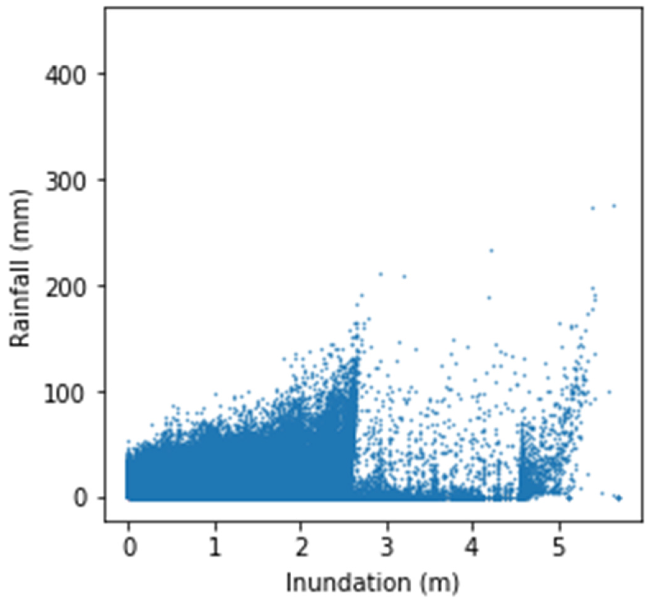
We assumed that the magnitude of flooding is directly related to the maximum flooding depth. Figure 2 illustrates the relationship between the maximum hourly rainfall and maximum flooding depth over the entire area for 218,850 datasets. Intuitively, the greater is the maximum rainfall, the greater is the maximum flood depth. However, Figure 2 shows that the data distribution is highly nonuniform, indicating that the relationship between two-dimensional rainfall and two-dimensional flood is a complex nonlinear problem. The factors influencing the flooding depth include the locations of maximum rainfall, geographic conditions, artificial structures, and other environmental factors.
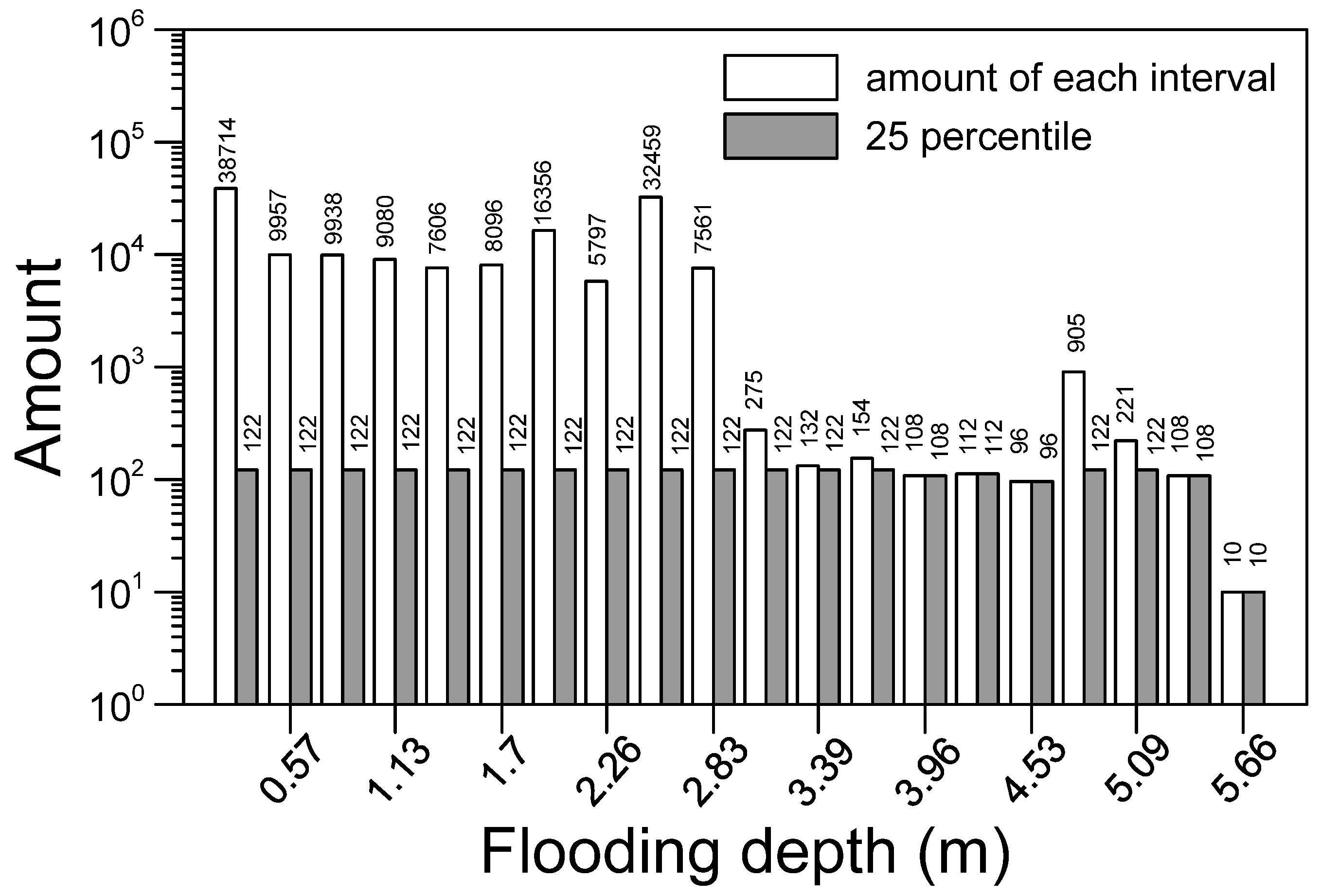
A relatively small amount of data had a maximum flooding depth ranging between 2.5 and 4.5 m; this may have been due to the random generation of data. Therefore, a method for sampling such nonuniform data had to be designed. Over-concentration or bias over some data interval would lead to unsatisfactory training results. Therefore, the maximum flooding depth in all datasets (i.e., 5.6571 m) was divided into 20 equal intervals, and the amount of data within each interval was calculated. Finally, 1447 datasets were randomly selected from the 25th percentile of the 20 intervals, as shown in Figure 3; these datasets accounted for 0.653% of all the training data. The 25th percentile was used because the data for the maximum flooding depth could be used as much as possible given the small amount of data for the smaller flooding depths. Additionally, the number of sampling data points for medium flooding depth should be similar to that for a low flooding depth. This preliminary study used the simple relationship between the maximum hourly rainfall and maximum flooding depth and sampled the data using percentiles. This data sampling method may not be the optimal approach in terms of the training results, but different data sampling methods can be investigated in the future.
3. Methods
This section describes the two CNN architectures used in this study, the data used for model training, and the method employed to evaluate model accuracy (when compared with actual data).
3.1. Convolutional Neural Networks
This study used CNNs, which have been proven successful in recognizing and classifying computer vision images. A CNN comprises multiple layers of neurons. Each layer is a nonlinear operation that performs a linear transformation on the previous layer’s output. These layers are mainly convolutional layers and pooling layers. Convolutional layers contain a set of filters with parameters that must be learned. Each filter slides along the width and height of the input volume and calculates the dot product between the input and the filter at each spatial position. Each neuron is connected to each neuron in the previous layer, called a fully connected layer. Using the convolution and merging process results, this layer classifies images into labels. Because of the layer’s tightly connected features, in TensorFlow [25], this layer is called the dense layer. A CNN’s fully connected part determines the most accurate weights through backpropagation. According to the weight received by each neuron, priority is provided to the most suitable label. Finally, the neurons “vote” on each label, and the vote winner is the classification decision [26].
Our networks were implemented with TensorFlow, and different rainfall datasets were combined, with spatial information as input tensors and flooding simulations as label tensors. We applied two deep learning architectures: the simple CNN (SCNN) and Inception architectures (Figure 4). The Inception architecture has more parameters than the SCNN architecture: 2,084,225 versus 4225, respectively. Inception [27] is a well-known CNN architecture inspired by the early network-in-network neural network architecture [28], and it contains several parallel branches.
We did not use pooling layers because they result in a shift-invariance property [29] when predicting the exact size of images. Different numbers of filters with a grid size of 1 × 1 or 3 × 3 were used for matching. We applied one layer of fully connected neurons of size 1. The resulting responses were converted into probability values. The minimum batch size was set to 2, and the weight decay was set to 10−6. We used the optimizer Adam [30] with a learning rate of 5 × 10⁻⁴ to train the network from scratch without utilizing pretrained model weights.
3.2. Data Combination for Training
Both CNN model architectures used two types of rainfall data, namely collocated coordinate, and elevation information, to generate different models. The rainfall data that corresponded to the earliest time point were those obtained in the 12th h (t = −11) before the time point of interest (t = 0). If all the hourly rainfall distribution data were used, the rainfall data occupied 12 CNN channels. When the number of channels is high, considerable computer and GPU memory are consumed. In general, digital image recognition datasets, the size of each image is 20 × 20 or 28 × 28 pixels, and the number of parameters is 4010 [31]; in addition, 60,000 and 10,000 images are employed for training and testing, respectively. The size of each map used in the present study was 360 × 201, which is approximately 92 times that of 28 × 28. When 12 h were considered, the number of single rainfall data reached 1107 times of a 28 × 28 pixels image. If a more extended period of rainfall is investigated in future studies, more memory will be required. Therefore, this study did not use all the rainfall data at each hour but instead used the data for some specific hours. Theoretically, relatively recent rainfall has a major impact on a flooding situation. Strategically, we thus did not sample rainfall data from a prior long period too densely and not too sparsely because the total accumulated rainfall was essential.
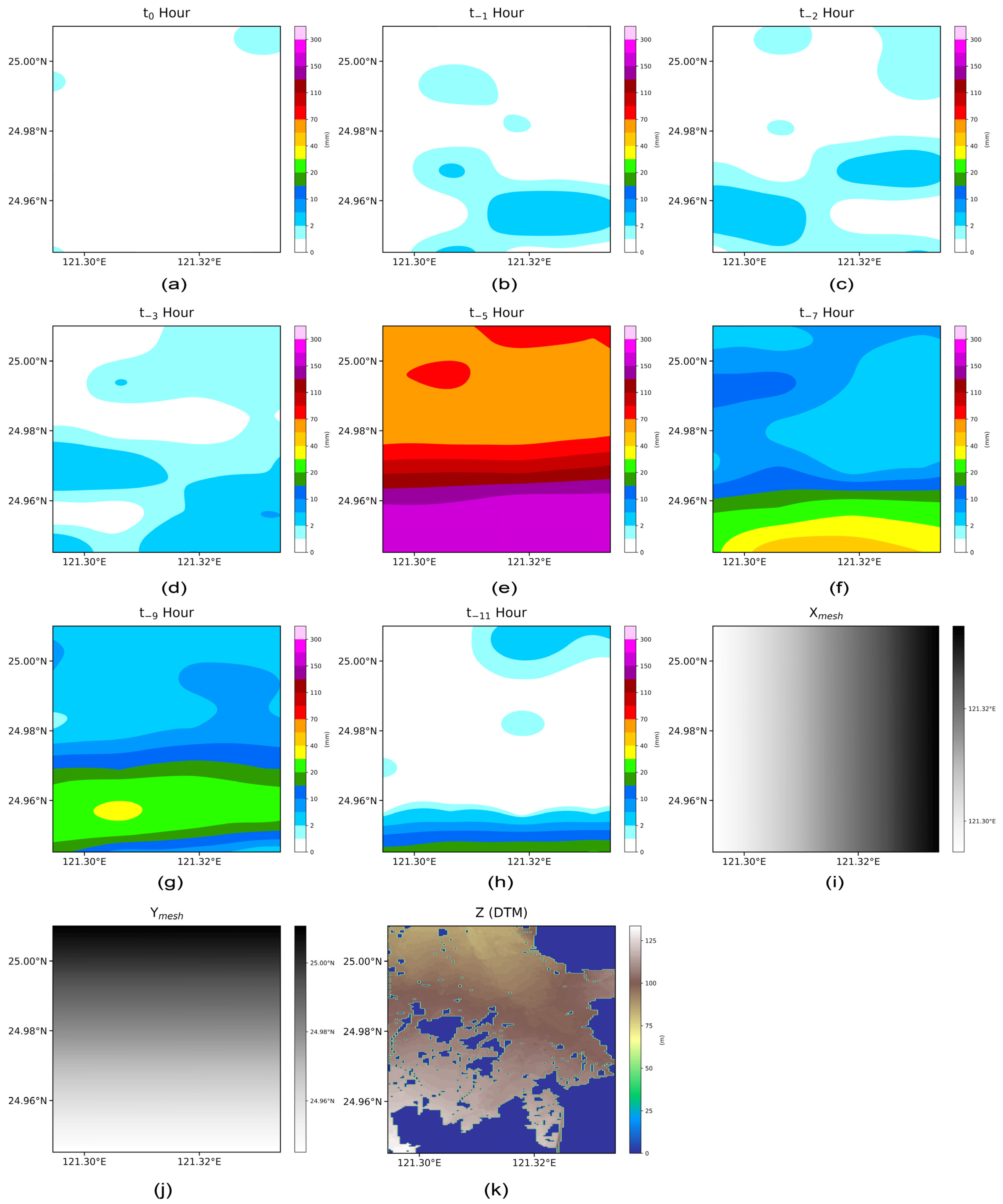
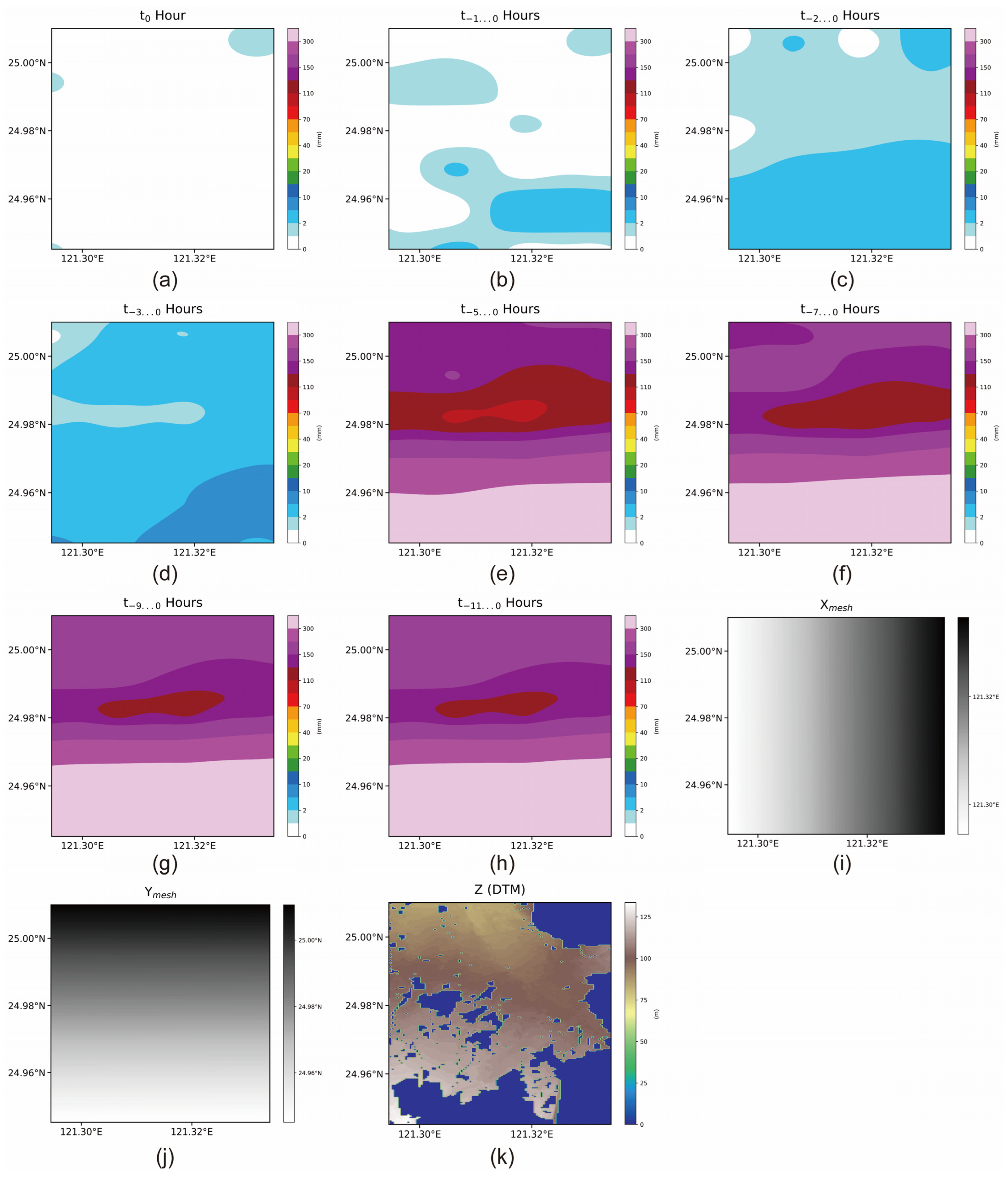
Considering these factors, the rainfall data for some specific hours were selected: those at t0, the most recent hour; t−1, the second most recent hour; t−2, the third most recent hour; t−3, the fourth most recent hour; t−5, the sixth most recent hour; t−7, the eighth most recent hour; t−9, the tenth most recent hour; and t−11, the twelfth most recent hour. A dataset contained rainfall data and grid and elevation information, as illustrated in Figure 5. To test the ability of the multichannel CNN model to memorize past rainfall data, the accumulated rainfall of different past periods was input into different channels for testing: these periods included t0, the most recent hour of rainfall; t−1,0, t−3,−2,−1, t−3,−2,…0, t−5,−4,…0, t−7,−6,…,0, t−9,−8,…,0; and t−11,−10,…,0, the most recent 2, 3, 4, 6, 8, 10, and 12 h of accumulated rainfall. The dataset contained accumulated rainfall data from the same data source as in Figure 5, grids, and the elevation information, as shown in Figure 6. The effects of the hourly versus accumulated rainfall data types on the CNN learning results were determined. It can be observed that several zero parts in the digital terrain model (DTM) map are used when simulating using the SOBEK model. These zero values indicate areas that have never been flooded or they are impossible to be. Henceforth, during the simulation, the elevation values are set to NaN, which is why the value seen in the graph is zero.
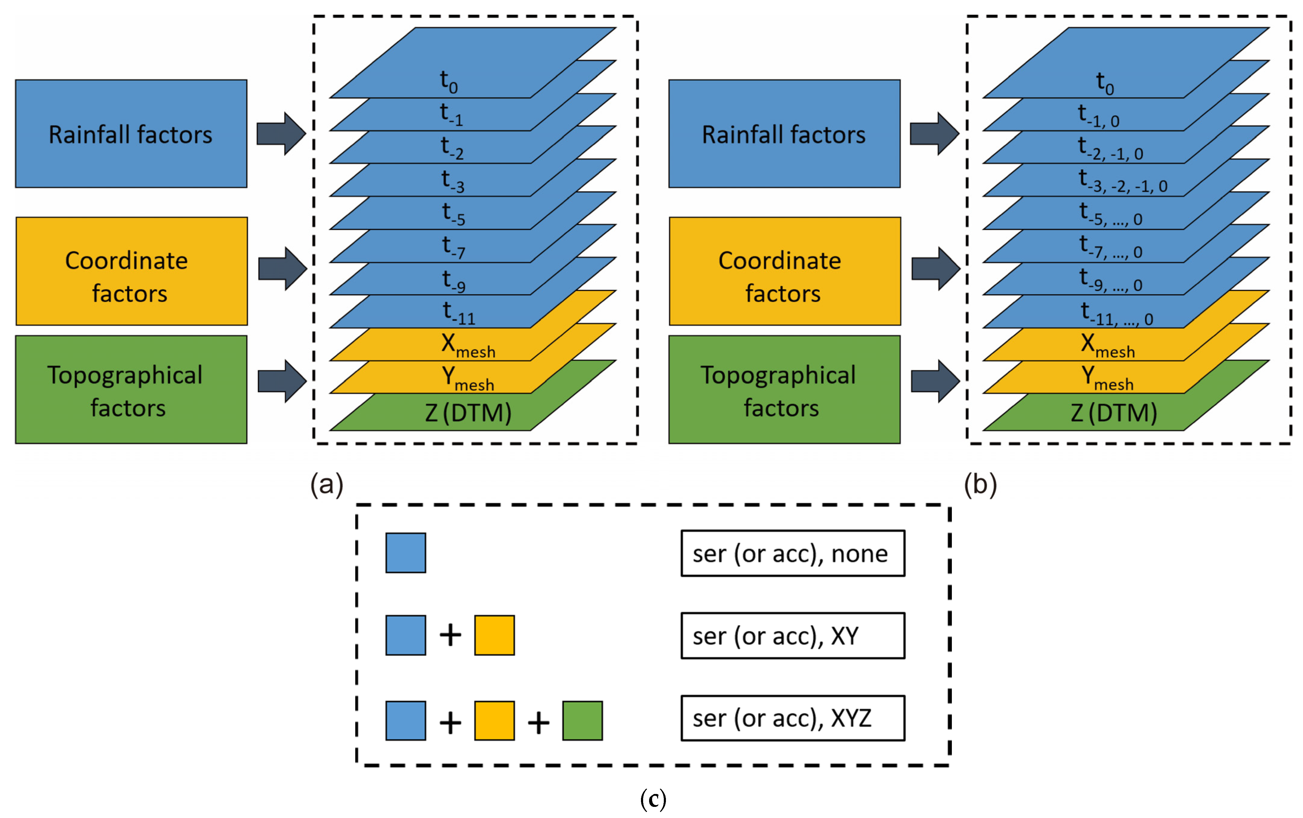
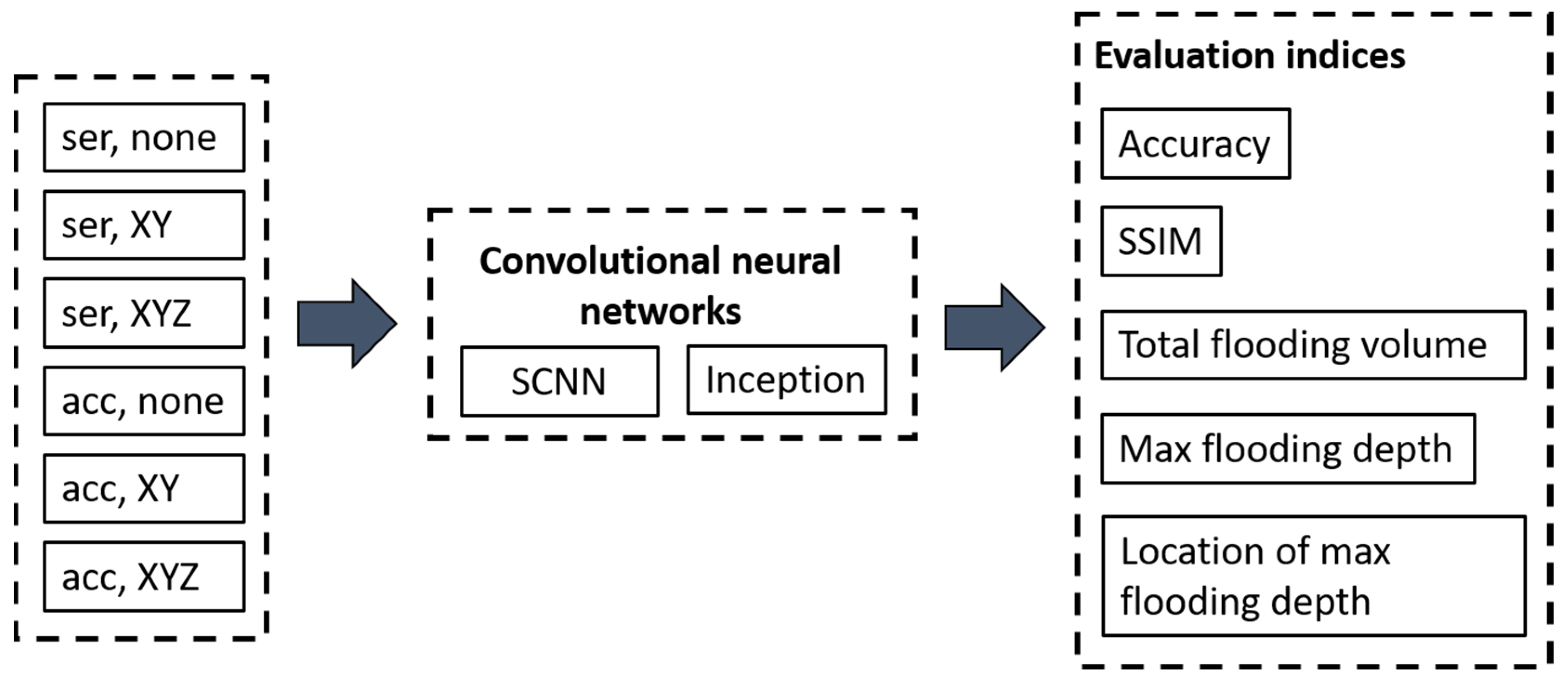
In this study, various combinations of different rainfall types, coordinates, and elevations were made, as shown in Figure 7. These combination data were input models (Figure 8) used to test the sensitivity of using a CNN. We employed 12 combinations in this study; the 12 models are shown in Table 3.
Model training was executed on the computing container of Taiwania2, which is an AI supercomputer built by the National Center for High-Performance Computing of NARLabs of the Ministry of Science and Technology. Different deep learning models use one to four GPUs; each GPU is equipped with four CPUs and 90 GB of memory. The GPU is NVIDIA V100 with 32 GB of memory.
3.3. Evaluation Methods
The comparison of two-dimensional data is more complicated than that of one-dimensional data; subjective visual comparison is often performed, or data at a specific location are chosen for comparison. Many scholars have proposed methods for evaluating their proposed two-dimensional models. Jamali et al. [19] employed five indices—the hit rate, false alarm rate, critical success index, root-mean-square error, and Nash–Sutcliffe efficiency—to compare the maximum flooding depth values with the results obtained using the HEC-RAS and TUFLOW models. However, the purpose of the present study was to predict not the maximum flooding depth for an entire rainfall event but rather the extent of flooding and the flooding depth over a specific time for the entire region. We needed to compare a time-by-time flooding map with the corresponding actual values. Comparison of the maximum flooding depth for an entire event would not be sufficient to demonstrate the performance of the method proposed in this paper. This study employed the structural similarity index (SSIM) [32] to conduct a comparative evaluation. In the SSIM, the indexing approach is used to implement the philosophy of structural similarity from the image formation perspective. Then, with four sets of results with high similarity, the differences in grid positions of the maximum flooding depths in all training data were compared. Finally, we identified the optimal model and compared its predicted maximum flooding depth with the actual data and the total flooded volume (including a comparison of training data and test data).
3.3.1. SSIM
The SSIM [32] is an objective method for assessing image quality. The differences between a distorted image and a reference image are obtained using various known properties of the human visual system. This approach is used to implement the philosophy of structural similarity from the image formation perspective. It can favorably identify similarity in an image structure. SSIM measurement involves three comparisons: those of luminance, contrast, and structure. In addition, the convergence conditions used in the training process and the illumination component of the graph similarity described as follows include the root-mean-square error and comparison of the flooding depth and flooding depth of the entire flooding range. The comparison of the flooding depth of the entire flooded area, the degree of contrast of flooding depths, and the distribution of the flooded area may provide relatively complete results.
Suppose x and y are two image signals which have been aligned with each other (e.g., spatial patches extracted from each image). The discrete signals are estimated as the mean intensity:
The standard deviation is used for estimating signal contrast, and the unbiased estimate in discrete form is given by
The signal is normalized by its standard deviation; thus, two compared signals have a unit standard deviation. The structure comparison is conducted on the normalized signals and .
Finally, the three components are combined into an overall measure of similarity:
The luminance comparison is defined as follows:
The contrast comparison function has a similar form:
The structure comparison function is as follows:
where the constants , , and are included to prevent the denominator being close to zero.
In discrete form, can be estimated as follows:
Geometrically, the correlation coefficient corresponds to the cosine of the angle between the vectors and .
The SSIM combines the three comparisons displayed in Equations (4)–(6):
where α > 0, β > 0, and γ > 0 are parameters used to adjust the relative importance of the three components. For simplicity, we set α = β = γ = 1.
3.3.2. Comparisons of Differences in Location for the Maximum Flooding Depth, Maximum Flooding Depth, and Total Flooding Volume
At the maximum depth, the grid difference between the case’s prediction model and the physical model was calculated as shown in Equation (9), and the result was then rounded to the nearest whole number.
The total flooded volume V was calculated as follows:
where , is the flooding depth of each grid cell, and and are the grid spaces of the x-axis and y-axis, respectively.
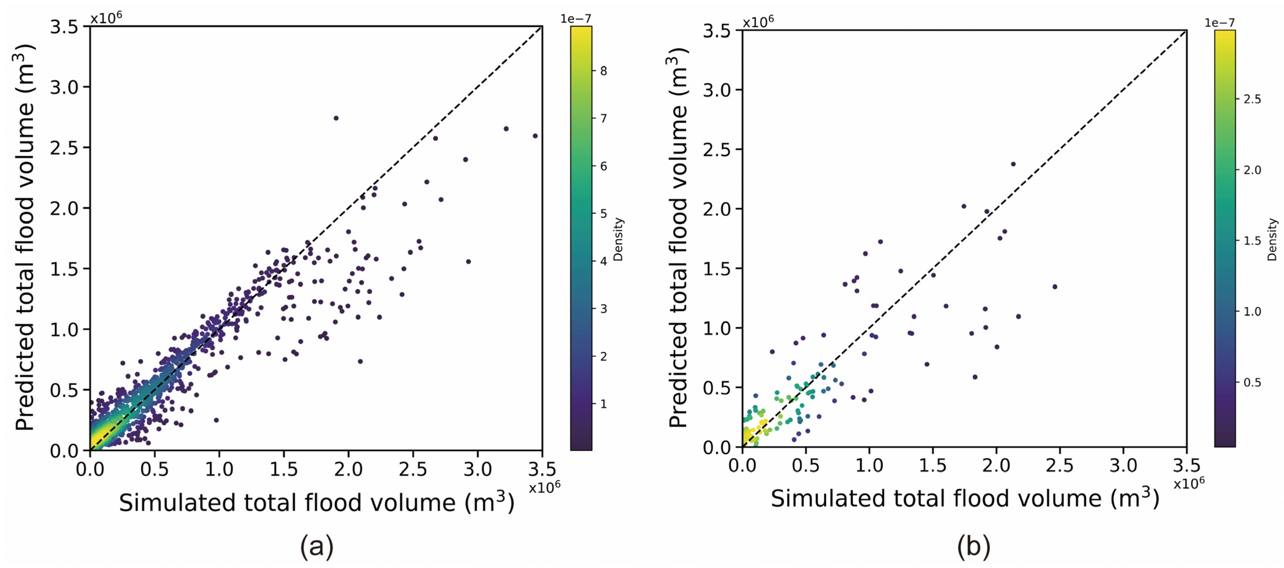
The total flooding volume in 1447 training data and 155 unused training data was compared with the result predicted using the AI model. Because of the excessive amount of data, the probability distribution function with the Gaussian distribution function as the kernel function to clarify the density of data [33].
4. Result Analysis
In this study, using the method described in Section 2.4, 1447 sets of rainfall data were extracted from abundant rainfall and flooding data, combining spatial XY and XYZ data, and were input to two CNN architectures (12 models) for training. A random 10% of the datasets was selected for validation. We thus employed 1302 datasets for training and 145 for validation during the training process. This section discusses the convergence of different data combinations under different CNN architectures.
Model Comparison
In the training process, the mean square error (MSE) was employed as the loss function. During the training process, the sum of the square of the distance between the predicted value and actual value was continually calculated as follows:
where is the actual value vector, and . is the predicted value vector.
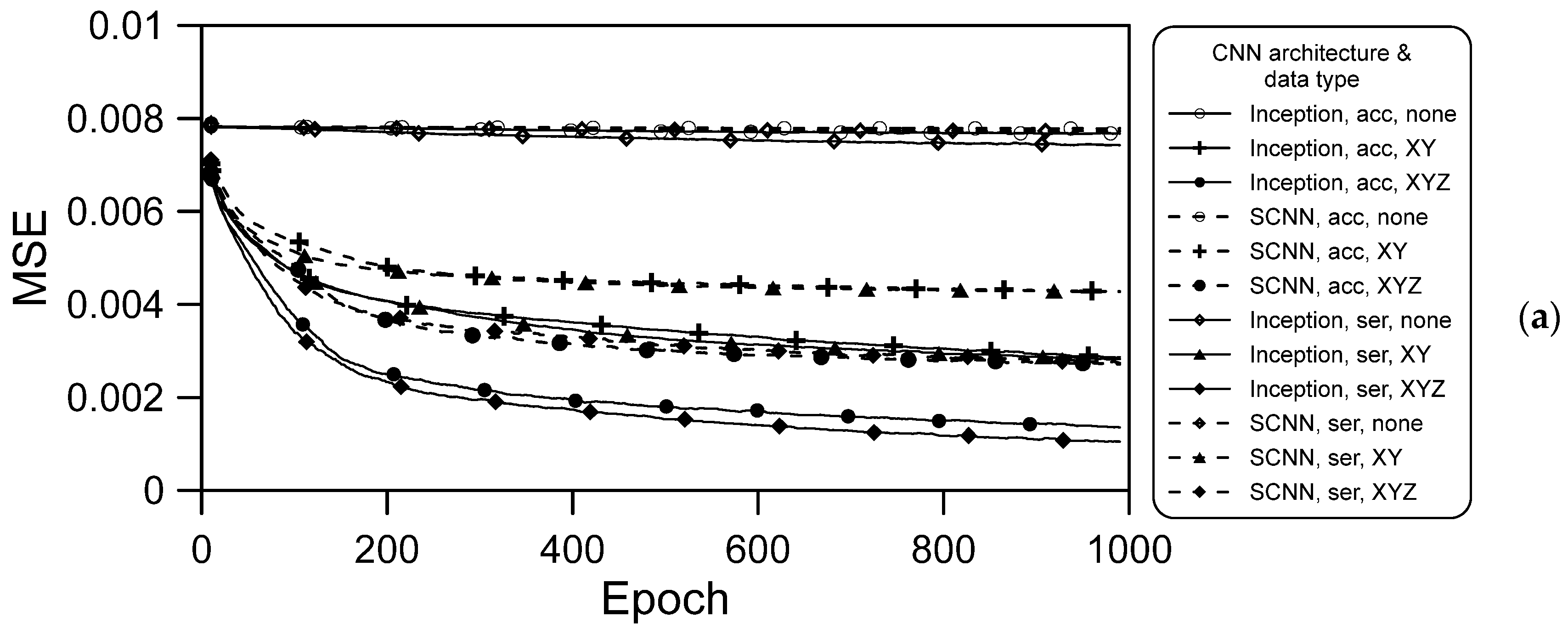
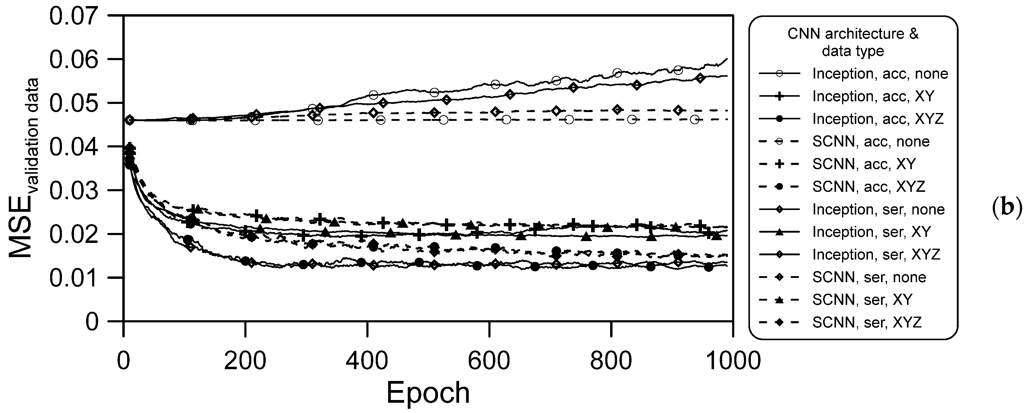
The MSE can reflect the actual situation of changes in training errors. The MSE results are presented in Figure 9 and can be summarized as follows:
- The training data not containing spatial information resulted in no convergence during the training process (Figure 9a), and the result obtained with the validation data was also divergent, as illustrated in Figure 9b. However, when spatial information was included, regardless of whether it was XY coordinates orYZ coordinates (including terrain elevation), convergence was gradually achieved in the training process;
- For both deep learning architectures and for both series hourly and accumulated rainfall data, the convergence obtained when XYZ spatial information was included was better than that achieved when XY spatial information only was included. Thus, elevation information is vital in CNN models used for flooding prediction;
- When the same data were used for training both architectures, convergence in the training was much better when using the Inception architecture than when using the SCNN architecture. We attribute this to the Inception architecture parameters being more numerous, which meant that more information was learned after separate training and merging of various training branches;
- For a given deep learning architecture and type of spatial information, the convergence achieved using the series hourly rainfall data was slightly better than that achieved using the accumulated rainfall data. For the training data, the effects of CNN architecture and spatial information type are stronger than that of rainfall data type.
These results indicated that although the input rainfall data were an array, the CNN architecture did not affect location learning. Coordinate information (XY) should at least be input to the model to the location of flooding.
We discuss the results of a comparison of the prediction results and case examples in the following section. Because convergence was not achieved when spatial data were not used in the training process, the four models without spatial data were not discussed in the subsequent analysis.
5. Discussion
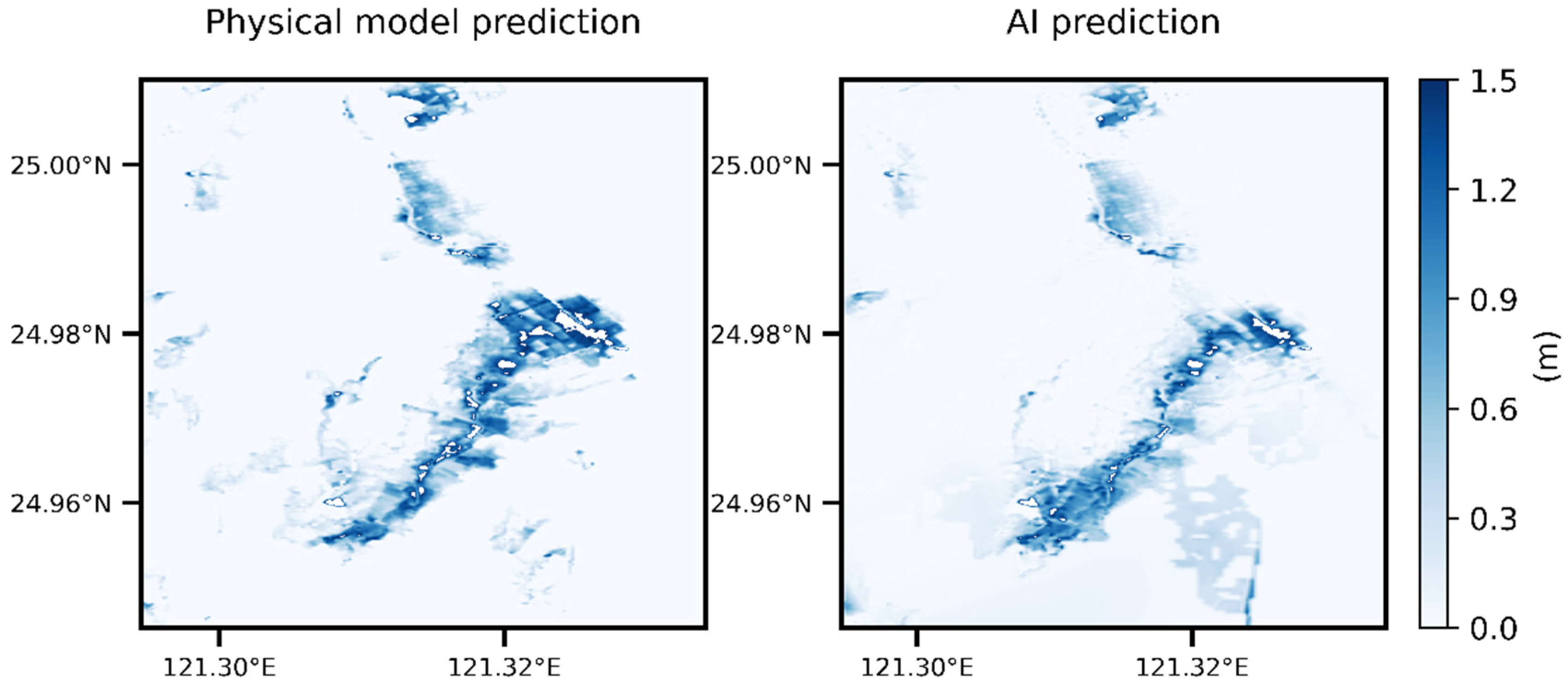
Figure 10 presents an example comparison of the AI prediction results. The training result is the two-dimensional flooding range and depth generated after inputting the spatial rainfall using the model established in this article. The actual value is the flooding simulation results of the physical flooding model used for training, corresponding to the same spatial and temporal rainfall. If the AI predictions were not specifically labelled, it would be difficult to detect them in the graph. Overall, the two plots of flooding distribution and depth are highly similar. Objective methods are needed to determine their difference. This study used the SSIM to determine the similarity of the two graphics (from the predicted and actual results). The SSIM can be divided into luminance, contrast, and structure comparisons. In the present context, these three comparison components constituted a comparison of the average flooding depth in the two graphs, a comparison of the contrast ratio of the two graphs, and a comparison of the flooding distribution’s structure in the two graphs. Then, the differences in the location at which the maximum depth occurred, in the maximum flooding depth over the entire area, and in the total flooding volume, were determined. Finally, the set of data for an event that was not included in the training data was used to obtain grid differences, the variation in the maximum flooding depth, and the variation in the flooding depth at some specific sites.
5.1. Similarity
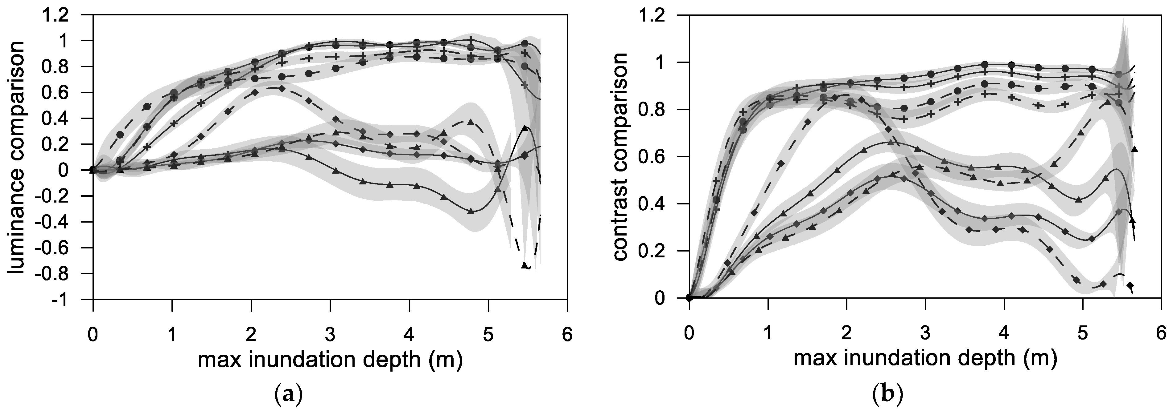
The 1447 training and validation rainfall datasets were used for comparing the various models constructed in this study. Because there are 1447 sets of data for each group of CNN models to compare the predicted results with the actual value, if each point is drawn on the graph, it will appear very messy and complicated to compare and read. Therefore, this study used a high-order polynomial method to regress each SSIM of the group model and the results of its components. The regression results for the SSIM and the index’s three components when high-order (10th-order) polynomials were fitted are shown in Figure 11; the shaded area indicates the 95% confidence interval. The results can be summarized as follows:
- For both the SCNN and Inception architectures, when the accumulated rainfall data were used, the luminance, contrast, structure, and final synthesis (SSIM) results were more favorable than those obtained when the hourly time-series rainfall data were employed;
- The similarity at a small flooding depth was not ideal because in the initial stage of flooding, few grids were flooded. The few numbers of flooded grids severely affected the similarity results. A possible way to improve this is to increase the amount of training data with a small flooding depth;
- When using the hourly time-series rainfall data as the training data, the similarity at various maximum flooding depths fluctuated and was nonuniform, regardless of whether the spatial information contained terrain elevation. Thus, neither architecture could stably learn the time-series rainfall data;
- Regardless of the deep learning architecture that was employed and whether hourly time-series or accumulated rainfall were used, the use of spatial information, including terrain elevation, led to much more favorable results than the nonuse of this information;
- A divergence was discovered near the maximum flooding depth. This was because when high-order polynomial regression is used, oscillation occurs at the edge of the interval; this is called the Runge phenomenon [34]. The phenomenon occurs when using polynomial interpolation with high-degree polynomials over a set of equally spaced interpolation points.
5.2. Comparison of Locations at Which Maximum Flooding Occurred
The most challenging part of verifying simulations of two-dimensional flooding is comparing the location at which the depth is the maximum at a specific time. The predicted location of the maximum flooding depth was compared with the actual value, and the grid difference was compared using Equation (9). The statistical results are plotted in Figure 12:
- The result obtained using the training data containing spatial information XYZ was far more accurate than that obtained using the training data containing only spatial information XY;
- The maximum position was found to be correct approximately 47% of the time. The grid position was within five grids of the actual position approximately 60% of the time; this percentage was much higher than 1/(360 × 201) = 1.38 × 10⁻⁵, indicating that the model could learn the flooding position and did not simply guess the location randomly.
Lower-lying areas are generally more prone to flooding. Our research demonstrated that neither CNN architecture could learn anything when the training data did not contain any coordinates. When the training data did contain the relevant coordinates, both CNN architectures could learn the correspondence between the flooding location and rainfall distribution, regardless of whether the training data contained elevation data. The learning of flooded areas was however more effective when the data included terrain elevation information.
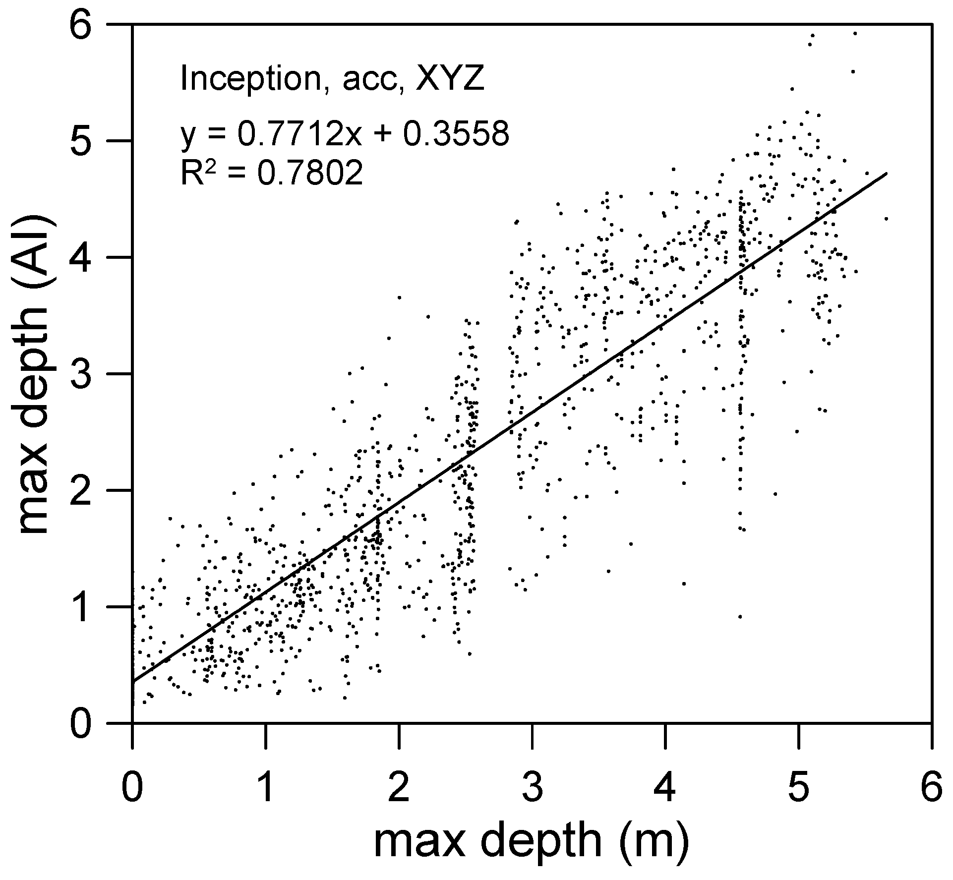
5.3. Maximum Flooding Depth Prediction
The similarity results indicated that the optimal model was that obtained when the accumulated rainfall data containing XYZ information was input into the Inception architecture. Figure 13 presents a comparison of the maximum flooding depth predicted by this optimal model with the actual data. The plot shows an excellent linear relationship; R2 is 0.78, but the regression line does not pass through the origin. A small value is present in the non-flooded area in the two-dimensional flooding-prediction map (and the minimum flooding depth in space). Thus, a numerical offset may exist in the deep learning regression result. The value shift may be due to the data sampling because we almost did not sample non-flooding data. The data for the first 11 h of each event, with little rain and no flooding, were not selected.
5.4. Total Flooding Volume
For the 1447 training datasets and 155 unused training datasets, the total flooding volume was calculated using Equation (10) and compared with the results predicted by the AI model, respectively. The findings are illustrated in Figure 14a,b. The predicted total flooding volume over the entire area was in favorable agreement with the actual data, regardless of whether the training data or testing data were employed. The predicted flooding volume was consistent with that obtained using the physical model.
5.5. Case Comparison
In addition to comparing the results of the models with the actual data, we compared the results of the models with the data that were not used for training. The optimal approach was to simulate a complete rainfall event to observe the entire process from the rising water levels to the eventually falling water levels.
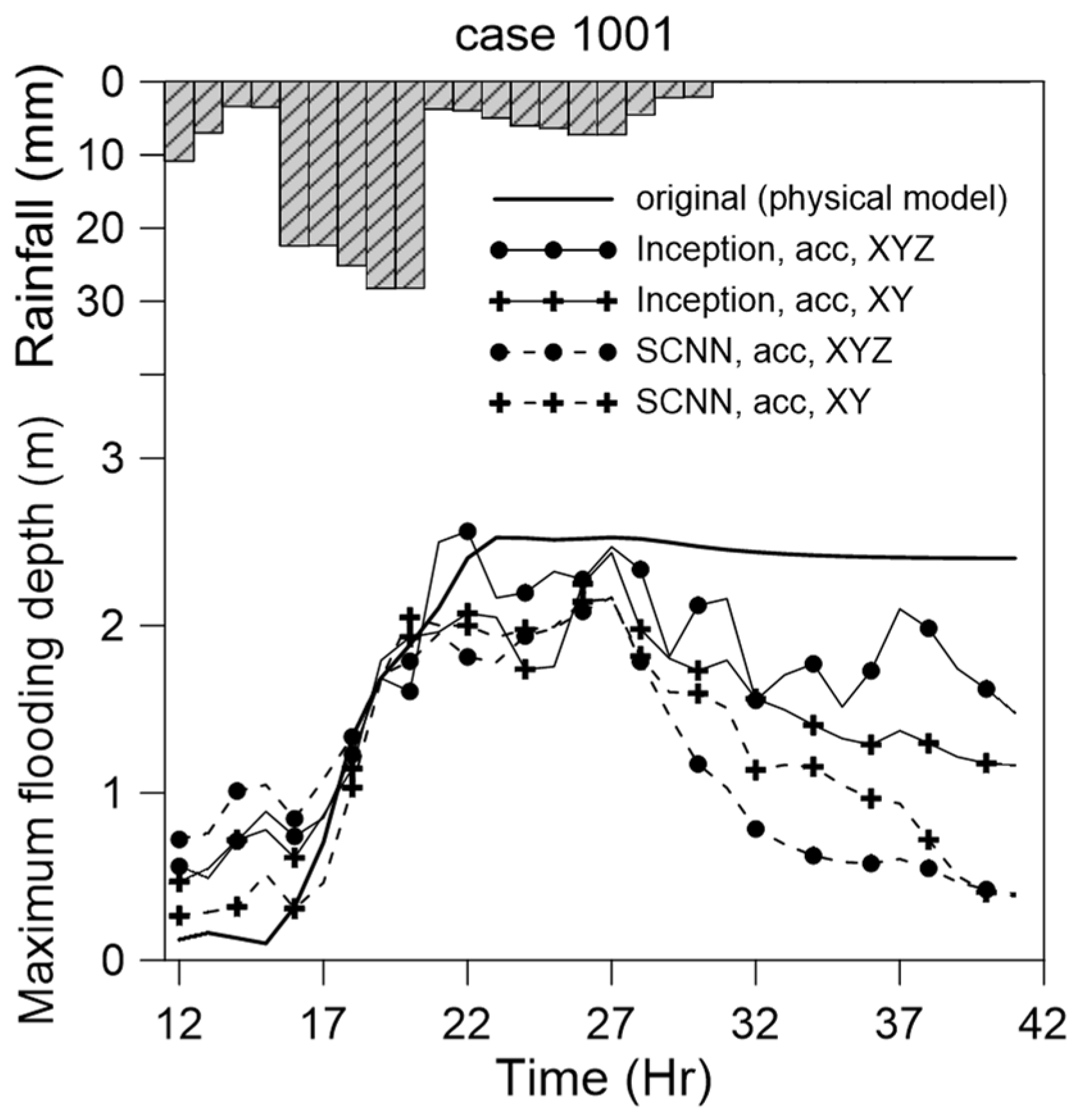
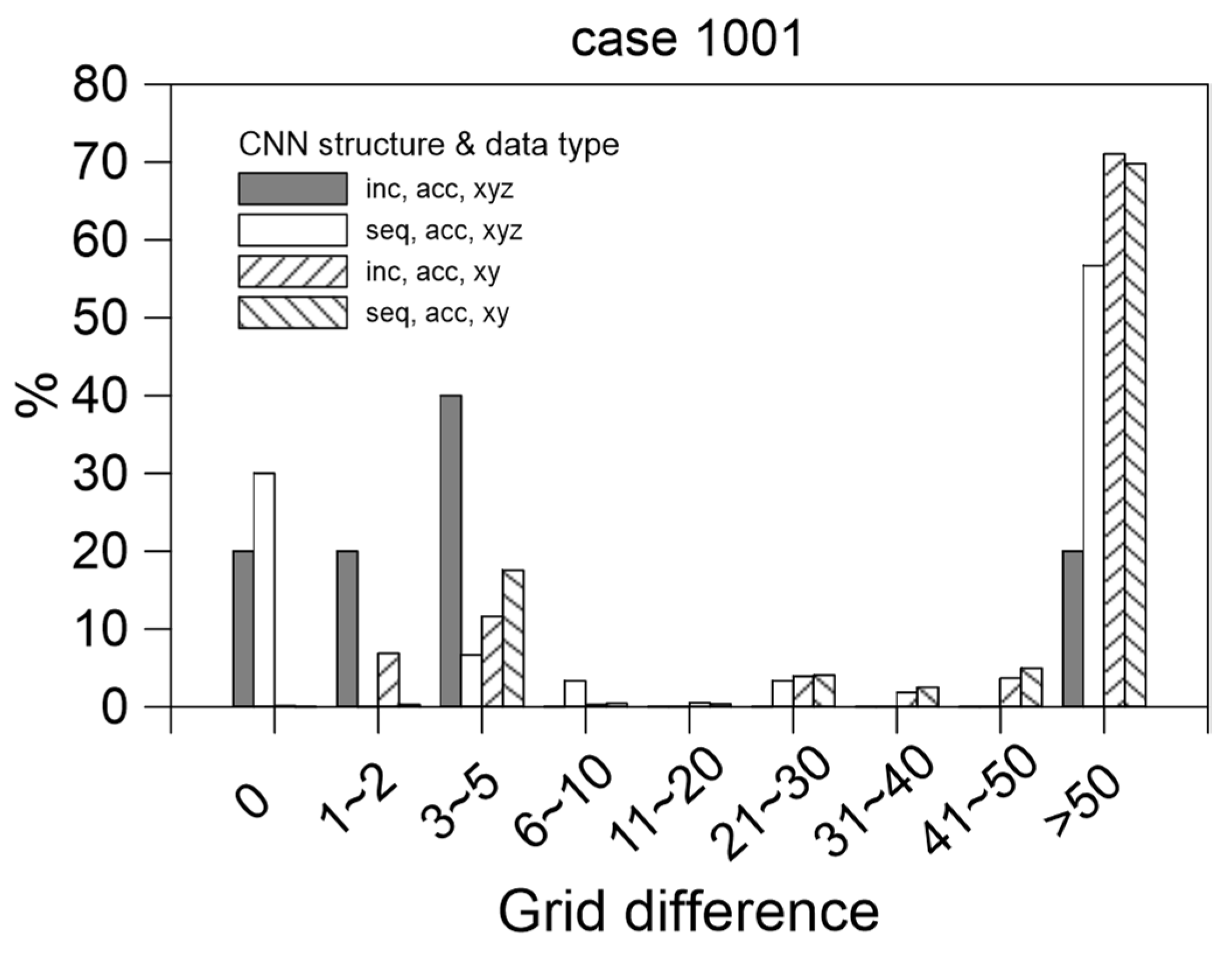
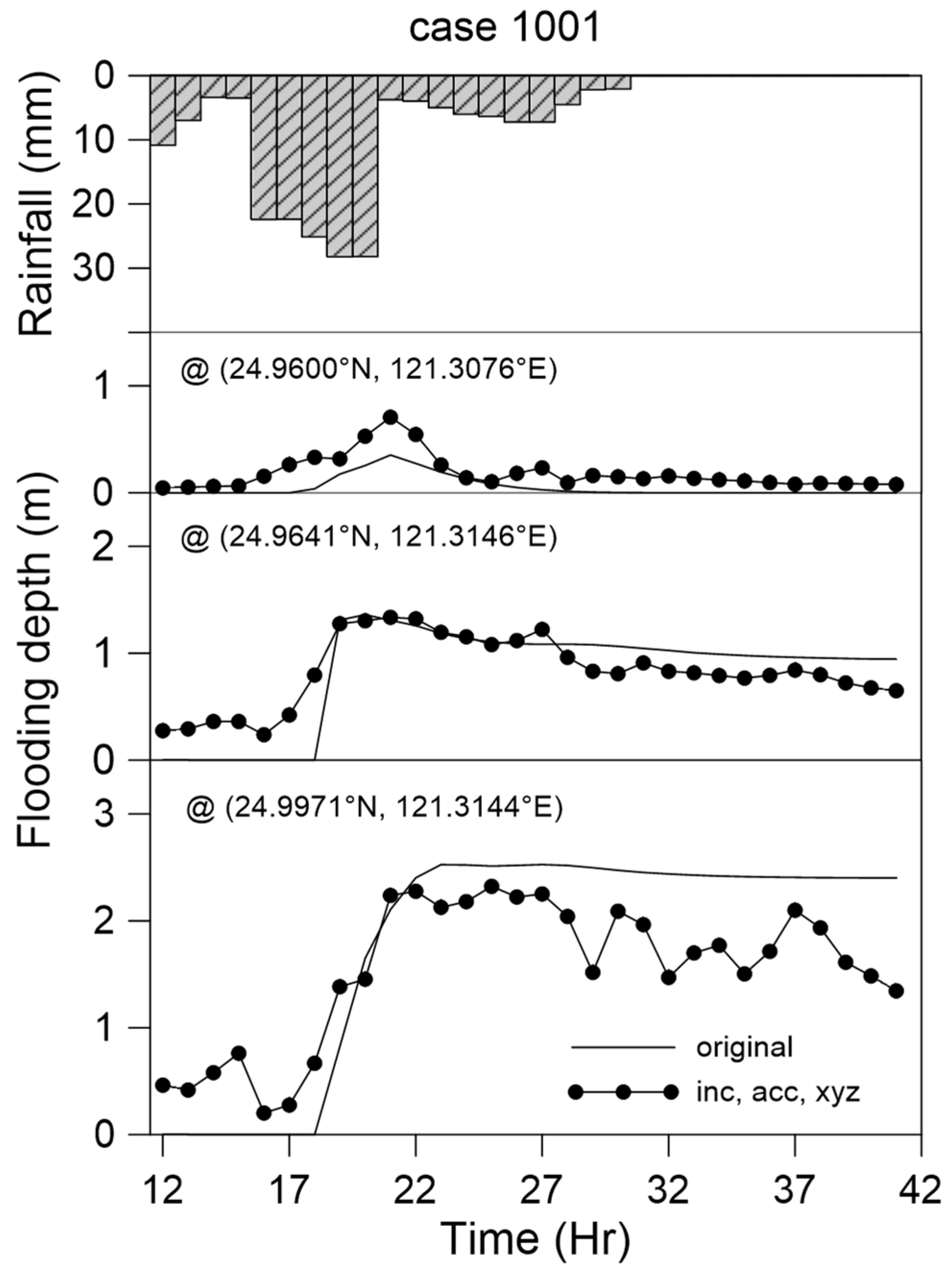
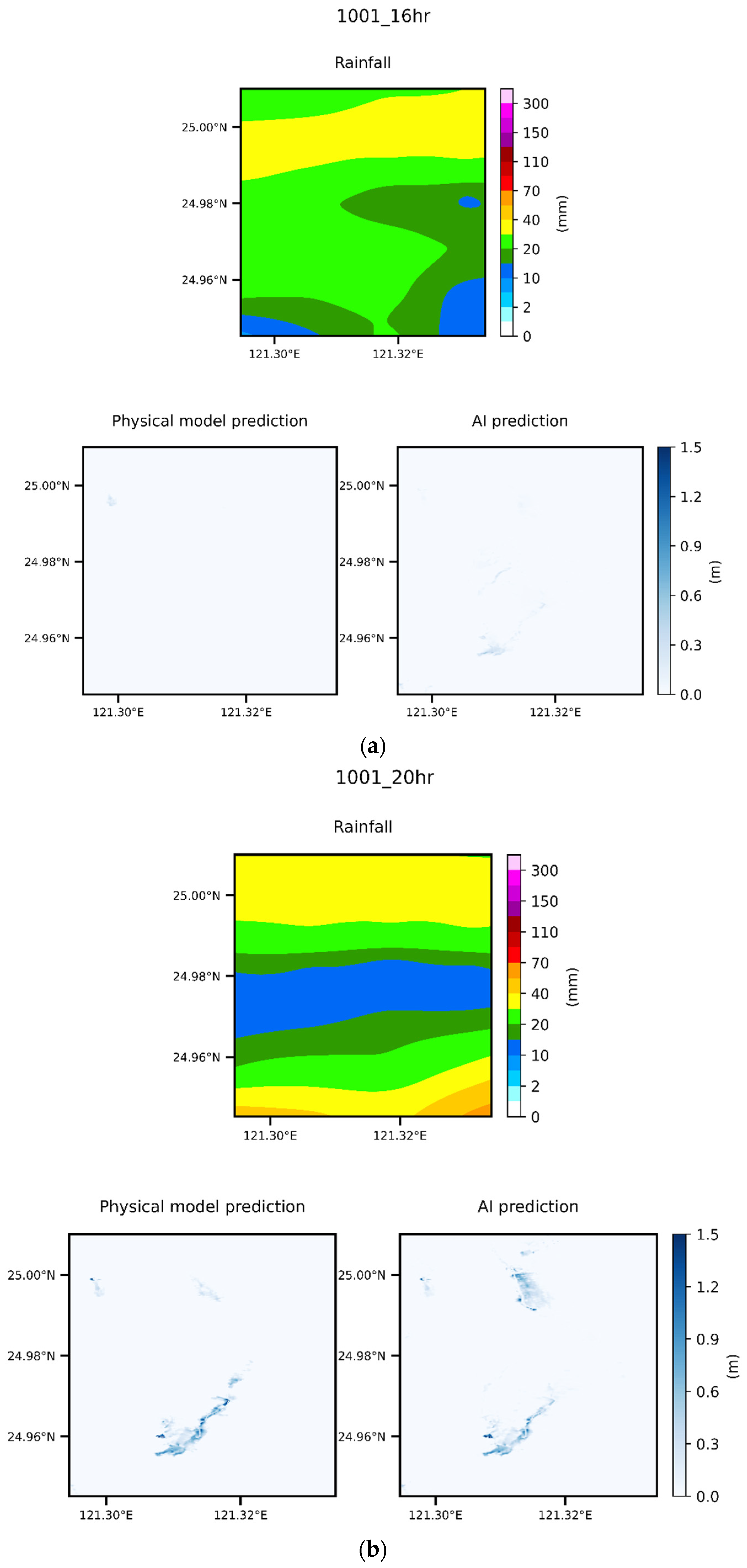
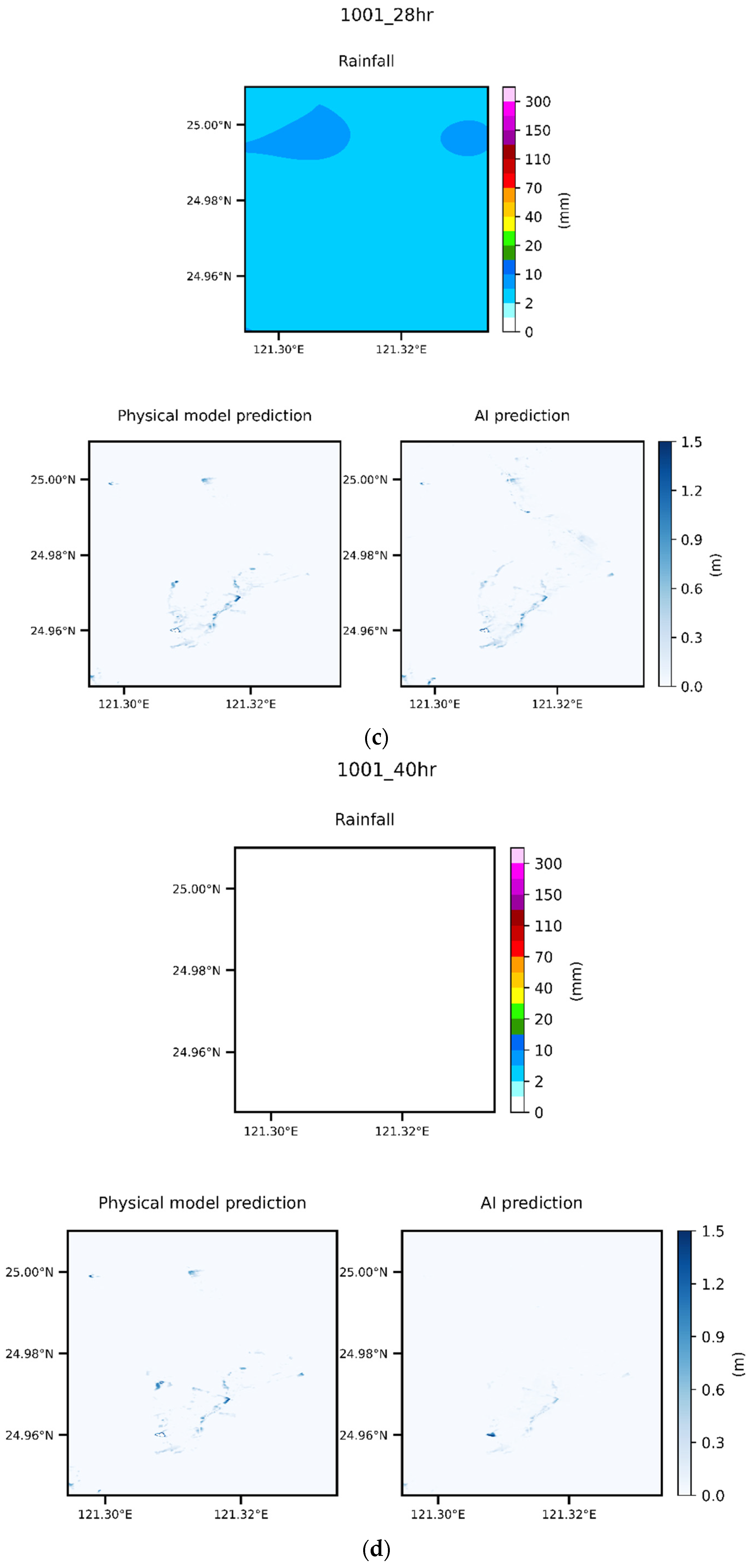
In this study, an event was randomly selected from the group of 6000 events; the data for this event were not included in the training data. We compared the maximum flooding depth variation within the flooding range using various models (Figure 15). The maximum flooding location’s grid difference varied with time, as illustrated by the statistics presented in Figure 16. Three specific locations were selected for comparisons of the flooding depth (Figure 17). The model and data combination selected was concluded to be optimal, given the results presented in Figure 11 and Figure 12. We still examined the overall spatial difference between the entire flooded area and the original scenario. We selected four time points for comparison (Figure 18). Finally, the difference between the prediction made using the deep learning model and the scenario event is plotted in Figure 19.
As presented in Figure 15, the results obtained using various models were consistent with the physical model results. The results of all models indicated that the water level gradually rose as the rainfall intensity increased, with the maximum flooding depth being reached at approximately the 22nd hour. The rainfall intensity then decreased, and the water level gradually receded. The receding of the water in each deep learning model was more evident than that in the physical model. The recession in the physical model was not apparent after a period of no rain. We attributed this to the physical model’s relevant regressive conditions not being fully set or the physical assumptions for the solution being incomplete. By contrast, the deep learning model predicted a receding period that was intuitively reasonable. This is because the sampled data were not divided into rising and falling water sections; only the relationship between rainfall intensity and flooding depth was considered. When the rainfall intensity was small in the input data, the corresponding flooding depth was small; thus, the water receding effect was correctly reflected. The deep learning results seemed to be in more favorable agreement with the physical phenomenon, even though the recession section of the physical model data seemed unreasonable. This study did not use flooding observation data for hourly correction of the flooding depth; only rainfall data were used as the input condition. This observation means that when our method predicts flooding in the long term, in addition to the range and magnitude of the flooding, it can predict the time point at which the water level will change from rising to falling.
The statistics for the grid difference in the position at which the maximum flooding depth occurred (Figure 16) indicate that the optimal result was the grid difference of 5 or smaller in approximately 70% of cases when using the Inception architecture with accumulated rainfall data containing XYZ coordinates. For this same model, the difference was greater than 50 for approximately 20% of the grids. The reason is that the location at which flooding is the greatest is relatively uncertain at the beginning of flooding, and the depth of this flooding is extremely small, as illustrated in Figure 12. The second optimal result was obtained using the SCNN architecture and the accumulated rainfall data containing XYZ coordinates. For the other conditions, the grid difference was considerable. This result indicated the considerable accuracy of the flooding location predictions obtained using deep learning. We concluded that the Inception architecture and the use of accumulated rainfall data containing XYZ information generated the optimal model.
The highest-performing model was employed to predict flooding depth changes at three locations. The maximum flooding depths at these three locations differed considerably (Figure 17). A complete description of the water depth at a specific location over time was obtained. The variations in the time to reach the maximum flooding depth and the times at which the water began to rise and fall, were all perfect.
The spatial flooding results at various time points during the selected event are displayed in Figure 18; these results were obtained using the Inception architecture and accumulated rainfall data containing XYZ information. We selected four flooding maps for different critical times: the starting point of flooding (16th hour); the time at which the flooding depth was the maximum (20th h); the time when the rainfall stopped (28th h); and a time point after the rain had ended (40th h). The flooding began (the 16th h) when the period of maximum rainfall began. At this time, the rainfall distribution was uneven, flooding was very shallow, and the location of the maximum flooding depth considerably differed. Figure 18b shows the maximum flooding depth; its location is close to that in the actual data when the flooding depth is close to its maximum over the entire event. At the end of rainfall (Figure 18c), the rainfall intensity was low, and the overall flooding distribution was similar. The flooding range and depth were slightly smaller, whereas the maximum flooding depth position was almost the same. The rainfall intensity shown in Figure 18d is zero, and the overall flooding range is much smaller than that at an earlier point. The flooding range predicted by the model was much smaller than the actual value, and the maximum flooding depth was also different.
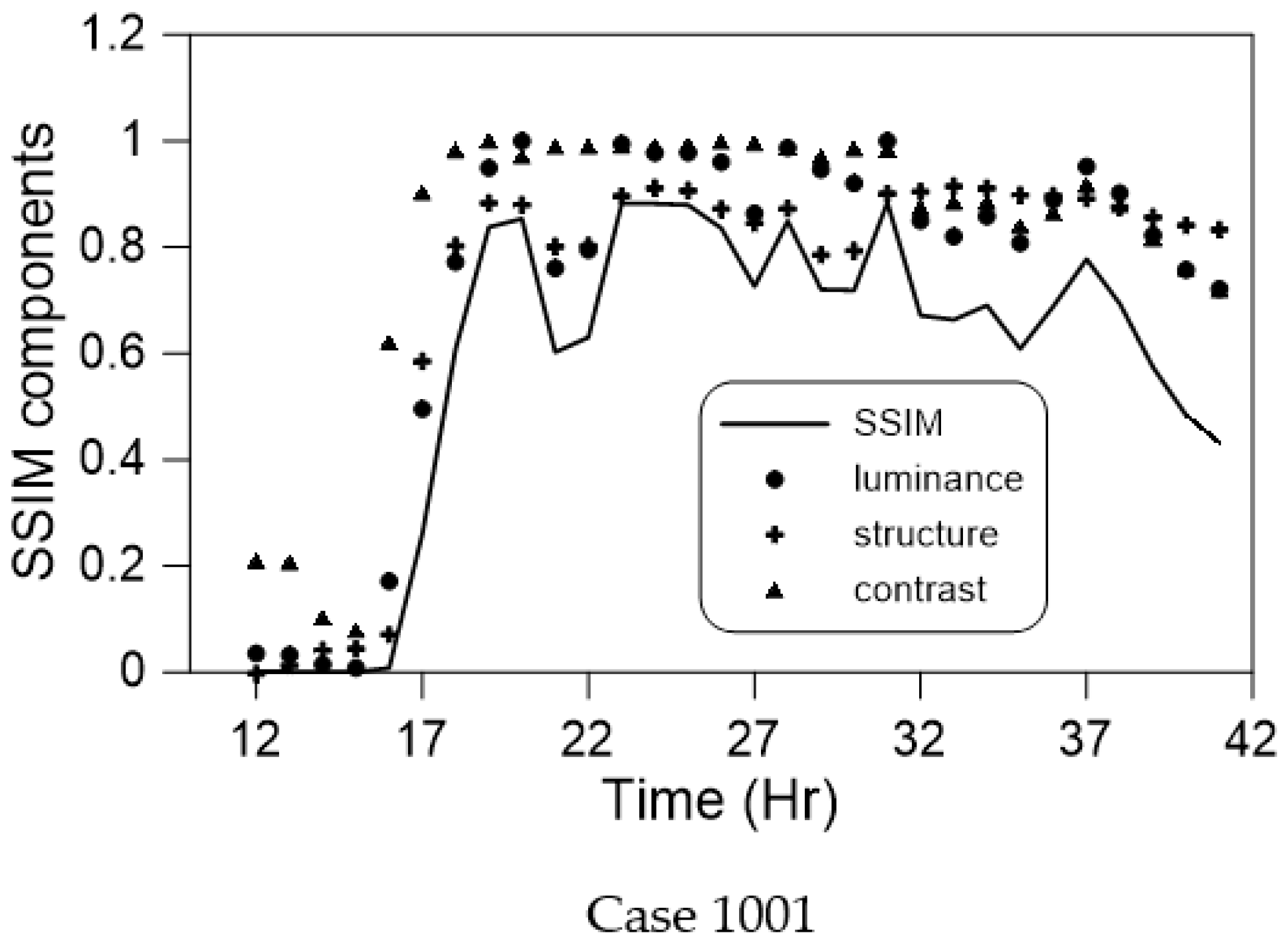
Finally, the similarity between the result of the deep learning model and the actual data throughout the event is illustrated in Figure 19. The similarity was the lowest in the early flooding stage but much higher when the flooding area was more extensive. Comparing the flooding range shown in Figure 18a, we came to the same conclusion as that in Section 5.1: the similarity was small because of the different positions of the grid points representing flooding. When the number of grids representing flooding became higher, favorable results were obtained regarding structure, intensity, and overall similarity. However, the low similarity during slight rainfall is not a concern during flooding.
6. Conclusions
This study proposed deep learning methods based on a CNN. Different spatial rainfall distribution data were combined to predict the corresponding two-dimensional flooding depth at various time points during flooding events. From the process and analysis of this research, the following conclusions can be drawn:
- This study used the SCNN architecture, which has few parameters, and the Inception architecture, which has numerous parameters, to make flooding predictions when training with the same data. The results revealed that the Inception architecture achieved excellent results;
- Using multiple and randomization methods, this study employed 21 actual rainfall events to produce 6000 rainfall events of various durations. The physical model we constructed could simulate a flooding situation under extreme rainfall. A total of 218,850 sets of rainfall data were generated from the data of 6000 events. We divided the maximum flooding depth of all data into 20 groups and calculated the amount of data in each group. Only 0.653% of all the data were taken out for training, and this achieved favorable results;
- When spatial information was not included in the training dataset, convergence could not be achieved with either CNN architecture. Inclusion of XYZ information in the training data resulted in optimal results;
- More accurate training results were obtained when using accumulated rainfall data than when using hourly time-series rainfall data;
- This study used the SSIM to compare the flooding results predicted by the AI and physical models. When the water level was low because there were few deep-water grid samples, the similarity was low, and some other errors that occurred were due to the Runge effect. In all the other findings, excellent graphical similarity was discovered. The results obtained using deep learning to predict the flooding range and depth were very similar to the original data. Therefore, the method proposed in this paper obtained favorable results when used to predict flooding caused by heavy rain;
- Because of the sampling of the training data, the overall predicted water depth slightly shifted. In the future, the accuracy for low water levels can be improved by increasing the amount of the low water level or early rainfall data through data resampling.
- The deep learning models proposed in this study were trained with rainfall data and corresponding flooding depth data but without real-time data, which could be used to modify the prediction results. Therefore, the forecasted rainfall data can be input into our models to obtain long-term flooding forecasts, which would aid in disaster prevention and response, and provide responders with more time to prepare.
Author Contributions
H.-W.W. conceived and designed the methodology, data analysis, and analyzed training results. G.-F.L. gave some significant suggestions. S.-J.W. produced rainfall data. C.-T.H. produced flooding data. All the authors contributed to the writing and editing of the manuscript. S.S.T. spent effort on reviewing and editing this article. All authors have read and agreed to the published version of the manuscript.
Funding
This study was partially supported by grants from the National Science and Technology Council of Taiwan (MOST-111-2221-E-492-001).
Data Availability Statement
Raw data were generated at National Center for High-Performance Computing, National Applied Research Laboratories. Derived data supporting the findings of this study are available from the corresponding author on request.
Acknowledgments
This study was partially supported by grants from the National Science and Technology Council of Taiwan (MOST-111-2221-E-492-001). We also thank Liao Yu-Hui for her assistance in drawing Figure 1. This manuscript was edited by Wallace Academic Editing.
Conflicts of Interest
The authors declare no conflict of interest.
References
- Karamuz, E.; Romanowicz, R.J.; Doroszkiewicz, J. The use of unmanned aerial vehicles in flood hazard assessment. J. Flood Risk Manag. 2020, 13, e12622. [Google Scholar] [CrossRef]
- Lee, I.; Kang, J.; Seo, G. Applicability Analysis of Ultra-Light UAV for Flooding Site Survey in South Korea. ISPRS Int. Arch. Photogramm. Remote Sens. Spat. Inf. Sci. 2013, 30, 185–189. [Google Scholar] [CrossRef] [Green Version]
- Schumann, G.J.P.; Muhlhausen, J.; Andreadis, K. The Value of a UAV-Acquired DEM for Flood Inundation Mapping and Modeling. EGU Gen. Assem. Conf. Abstr. 2016, 18, EPSC2016–EPSC10158. [Google Scholar]
- Salmoral, G.; Rivas-Casado, M.; Muthusamy, M.; Butler, D.; Menon, P.P.; Leinster, P. Guidelines for the use of unmanned aerial systems in flood emergency response. Water 2020, 12, 521. [Google Scholar] [CrossRef] [Green Version]
- Teng, J.; Jakeman, A.J.; Vaze, J.; Croke, B.F.W.; Dutta, D.; Kim, S. Flood inundation modelling: A review of methods, recent advances and uncertainty analysis. Environ. Model. Softw. 2017, 90, 201–216. [Google Scholar] [CrossRef]
- Fernández-Pato, J.; Caviedes-Voullième, D.; García-Navarro, P. Rainfall/runoff simulation with 2D full shallow water equations: Sensitivity analysis and calibration of infiltration parameters. J. Hydrol. 2016, 536, 496–513. [Google Scholar] [CrossRef]
- Kim, B.; Sanders, B.F.; Famiglietti, J.S.; Guinot, V. Urban flood modeling with porous shallow-water equations: A case study of model errors in the presence of anisotropic porosity. J. Hydrol. 2015, 523, 680–692. [Google Scholar] [CrossRef] [Green Version]
- Cea, L.; Garrido, M.; Puertas, J. Experimental validation of two-dimensional depth-averaged models for forecasting rainfall–runoff from precipitation data in urban areas. J. Hydrol. 2010, 382, 88–102. [Google Scholar] [CrossRef]
- Costabile, P.; Macchione, F. Enhancing river model set-up for 2-D dynamic flood modelling. Environ. Model. Softw. 2015, 67, 89–107. [Google Scholar] [CrossRef]
- Leandro, J.; Chen Albert, S.; Djordjević, S.; Savić Dragan, A. Comparison of 1D/1D and 1D/2D coupled (Sewer/Surface) hydraulic models for urban flood simulation. J. Hydraul. Eng. 2009, 135, 495–504. [Google Scholar] [CrossRef]
- Guidolin, M.; Chen, A.S.; Ghimire, B.; Keedwell, E.C.; Djordjević, S.; Savić, D.A. A weighted cellular automata 2D inundation model for rapid flood analysis. Environ. Model. Softw. 2016, 84, 378–394. [Google Scholar] [CrossRef]
- Lohani, A.K.; Goel, N.; Bhatia, K. Improving real time flood forecasting using fuzzy inference system. J. Hydrol. 2014, 509, 25–41. [Google Scholar] [CrossRef]
- Rezaeianzadeh, M.; Tabari, H.; Yazdi, A.A.; Isik, S.; Kalin, L. Flood flow forecasting using ANN, ANFIS and regression models. Neural Comput. Appl. 2014, 25, 25–37. [Google Scholar] [CrossRef]
- Elsafi, S.H. Artificial Neural Networks (ANNs) for flood forecasting at Dongola Station in the River Nile, Sudan. Alex. Eng. J. 2014, 53, 655–662. [Google Scholar] [CrossRef]
- Choubin, B.; Moradi, E.; Golshan, M.; Adamowski, J.; Sajedi-Hosseini, F.; Mosavi, A. An ensemble prediction of flood susceptibility using multivariate discriminant analysis, classification and regression trees, and support vector machines. Sci. Total Environ. 2019, 651, 2087–2096. [Google Scholar] [CrossRef]
- Khosravi, K.; Pham, B.T.; Chapi, K.; Shirzadi, A.; Shahabi, H.; Revhaug, I.; Prakash, I.; Bui, D.T. A comparative assessment of decision trees algorithms for flash flood susceptibility modeling at Haraz watershed, northern Iran. Sci. Total Environ. 2018, 627, 744–755. [Google Scholar] [CrossRef]
- Tehrany, M.S.; Pradhan, B.; Mansor, S.; Ahmad, N. Flood susceptibility assessment using GIS-based support vector machine model with different kernel types. Catena 2015, 125, 91–101. [Google Scholar] [CrossRef]
- Zhao, G.; Pang, B.; Xu, Z.; Peng, D.; Zuo, D. Urban flood susceptibility assessment based on convolutional neural networks. J. Hydrol. 2020, 590, 125235. [Google Scholar] [CrossRef]
- Jamali, B.; Bach, P.M.; Cunningham, L.; Deletic, A. A cellular automata fast flood evaluation (CA-ffé) model. Water Resour. Res. 2019, 55, 4936–4953. [Google Scholar] [CrossRef] [Green Version]
- Guo, Z.; Leitão, J.P.; Simões, N.E.; Moosavi, V. Data-driven flood emulation: Speeding up urban flood predictions by deep convolutional neural networks. J. Flood Risk Manag. 2021, 14, e12684. [Google Scholar] [CrossRef]
- Berkhahn, S.; Fuchs, L.; Neuweiler, I. An ensemble neural network model for real-time prediction of urban floods. J. Hydrol. 2019, 575, 743–754. [Google Scholar] [CrossRef]
- Chang, L.C.; Shen, H.Y.; Chang, F.J. Regional flood inundation nowcast using hybrid SOM and dynamic neural networks. J. Hydrol. 2014, 519, 476–489. [Google Scholar] [CrossRef]
- Wu, S.J.; Tung, Y.K.; Yang, J.C. Stochastic generation of hourly rainstorm events. Stoch. Environ. Res. Risk Assess. 2006, 21, 195–212. [Google Scholar] [CrossRef]
- Wu, S.J.; Hsu, C.T.; Chang, C.H. Stochastic modelling of gridded short-term rainstorms. Hydrol. Res. 2021, 52, 876–904. [Google Scholar] [CrossRef]
- Abadi, M.; Barham, P.; Chen, J.; Chen, Z.; Davis, A.; Dean, J.; Devin, M.; Ghemawat, S.; Irving, G.; Isard, M.; et al. TensorFlow: A System for Large-Scale Machine Learning. In Proceedings of the 12th USENIX Conference on Operating Systems Design and Implementation, Savannah, GA, USA, 2–4 November 2016; pp. 265–283. [Google Scholar]
- Aghdam, H.; Heravi, E. Guide to Convolutional Neural Networks: A Practical Application to Traffic-Sign Detection and Classification; Springer: Berlin/Heidelberg, Germany, 2017. [Google Scholar] [CrossRef]
- Szegedy, C.; Vanhoucke, V.; Ioffe, S.; Shlens, J.; Wojna, Z. Rethinking the Inception Architecture for Computer Vision. In Proceedings of the 2016 IEEE Conference on Computer Vision and Pattern Recognition (CVPR), Las Vegas, NV, USA, 27–30 June 2016; pp. 2818–2826. [Google Scholar] [CrossRef] [Green Version]
- Min, L.; Qiang, C.; Shuicheng, Y. Network in network. arXiv 2014, arXiv:1312.4400. [Google Scholar] [CrossRef]
- Scherer, D.; Müller, A.; Behnke, S. Evaluation of pooling operations in convolutional architectures for object recognition. In Artificial Neural Networks–ICANN 2010-Lecture Notes in Computer Science; Diamantaras, K., Duch, W., Iliadis, L.S., Eds.; ICANN, Springer: Berlin/Heidelberg, Germany, 2010. [Google Scholar]
- Kingma, D.; Ba, J. Adam: A Method for Stochastic Optimization. International Conference on Learning Representations. arXiv 2014, arXiv:1412.6980v9 2014. [Google Scholar] [CrossRef]
- LeCun, Y.; Jackel, L.D.; Bottou, L.; Cortes, C.; Denker, J.S.; Drucker, H.; Guyon, I.; Muller, U.A.; Sackinger, E.; Simard, P.; et al. Learning algorithms for classification: A comparison on handwritten digit recognition. Neural Netw. Stat. Mech. Perspective 1995, 261, 2. [Google Scholar]
- Wang, Z.; Bovik, A.C.; Sheikh, H.R.; Simoncelli, E.P. Image quality assessment: From error visibility to structural similarity. IEEE Trans. Image Process. 2004, 13, 600–612. [Google Scholar] [CrossRef]
- Gutierrez-Osuna, R. Lecture notes in Kernel Density Estimation for CSCE 666: Pattern Analysis at Texas A&M University. 2020. Available online: https://pdf4pro.com/view/l7-kernel-density-estimation-texas-a-amp-m-university-5b8da8.html (accessed on 17 December 2022).
- Runge, C. Über empirische Funktionen und die Interpolation zwischen äquidistanten Ordinaten. Z. Fur. Math. Phys. 1901, 46, 224–243. [Google Scholar]
Figure 1.
Flooding simulation area: the Dongmen drainage.

Figure 2.
Relationship between maximum 1-h rainfall and maximum flooding depth.

Figure 3.
Original amount of data in various flooding depth ranges and the amount of 25th percentile data.
Figure 3.
Original amount of data in various flooding depth ranges and the amount of 25th percentile data.

Figure 4.
Two convolutional neural network (CNN) architectures: (a) Simple CNN; and (b) Inception.

Figure 5.
Schematic of the data combination, with the data being 8-h rainfall, X and Y meshes, and a digital terrain model. (a) the most recent hour rainfall; (b) the second most recent hour rainfall; (c) the third most recent hour; (d) the fourth most recent hour rainfall; (e) the sixth most recent hour rainfall; (f) the eighth most recent hour rainfall; (g) the tenth most recent hour rainfall; (h) the twelfth most recent hour; (i) the longitude mesh; (j) the latitude mesh; (k) elevation information.

Figure 6.
Schematic of the data combination, with data being 8-h accumulated rainfall, X and Y meshes, and a digital terrain model. (a) the most recent hour rainfall; (b) the most recent 2 h of accumulated rainfall; (c) the most recent 3 h of accumulated rainfall; (d) the most recent 4 h of accumulated rainfall; (e) the most recent 6 of accumulated rainfall; (f) the most recent 8 h of accumulated rainfall; (g) the most recent 10 h of accumulated rainfall; (h) the most recent 12 h of accumulated rainfall; (i) the longitude mesh; (j) the latitude mesh; (k) elevation information.

Figure 7.
Combination classification of: (a) rainfall data in different time series (ser), coordinates (XY), and elevation (Z); and (b) cumulative rainfall data in different periods (acc), coordinates (XY), and elevation (Z). (c) Combination of different physical factors.
Figure 7.
Combination classification of: (a) rainfall data in different time series (ser), coordinates (XY), and elevation (Z); and (b) cumulative rainfall data in different periods (acc), coordinates (XY), and elevation (Z). (c) Combination of different physical factors.

Figure 8.
Data of different combinations are input to two CNN architectures (SCNN and Inception). The obtained results are compared in various ways.
Figure 8.
Data of different combinations are input to two CNN architectures (SCNN and Inception). The obtained results are compared in various ways.

Figure 9.
Convergence of the loss function for different models: (a) training data; and (b) validation data.
Figure 9.
Convergence of the loss function for different models: (a) training data; and (b) validation data.


Figure 10.
Actual data (left) and deep learning predictions (right) of the flooding distribution and depth.
Figure 10.
Actual data (left) and deep learning predictions (right) of the flooding distribution and depth.

Figure 11.
Structural similarity index (SSIM) similarity in the flood results produced by various models to the corresponding actual data: (a) luminance comparison, (b) contrast comparison, (c) structure comparison, and (d) SSIM comparison.
Figure 11.
Structural similarity index (SSIM) similarity in the flood results produced by various models to the corresponding actual data: (a) luminance comparison, (b) contrast comparison, (c) structure comparison, and (d) SSIM comparison.


Figure 12.
Difference in the location of the maximum flooding depth between the actual data and the predictions made by the artificial intelligence (AI) models.
Figure 12.
Difference in the location of the maximum flooding depth between the actual data and the predictions made by the artificial intelligence (AI) models.

Figure 13.
Maximum flooding depth predicted by AI versus the actual data.

Figure 14.
Total flooding volume predicted by AI versus the actual values: (a) training data and (b) testing data.
Figure 14.
Total flooding volume predicted by AI versus the actual values: (a) training data and (b) testing data.

Figure 15.
Use of various deep learning models for a single rainfall event, showing the maximum flooding depth versus time.
Figure 15.
Use of various deep learning models for a single rainfall event, showing the maximum flooding depth versus time.

Figure 16.
Difference in the maximum flooding depth position when using various deep learning models to make predictions for a single rainfall event.
Figure 16.
Difference in the maximum flooding depth position when using various deep learning models to make predictions for a single rainfall event.

Figure 17.
Flooding depth at different locations versus time for a single rainfall event when using the Inception architecture and rainfall data containing XYZ information.
Figure 17.
Flooding depth at different locations versus time for a single rainfall event when using the Inception architecture and rainfall data containing XYZ information.

Figure 18.
Two-dimensional results obtained using the Inception architecture and accumulated rainfall data containing XYZ information in comparison with the physical model results at time points of (a) 16; (b) 20; (c) 28; and (d) 40 h.
Figure 18.
Two-dimensional results obtained using the Inception architecture and accumulated rainfall data containing XYZ information in comparison with the physical model results at time points of (a) 16; (b) 20; (c) 28; and (d) 40 h.


Figure 19.
SSIM and its components’ variation with time in the flooding results for a rainfall event when using the Inception architecture and accumulated rainfall data containing XYZ information.
Figure 19.
SSIM and its components’ variation with time in the flooding results for a rainfall event when using the Inception architecture and accumulated rainfall data containing XYZ information.


Table 1.
Actual rainfall events used for increasing the number of rainfall events.
| Event | Start Time | End Time | Duration (h) | Areal Average Rainfall (mm) |
|---|---|---|---|---|
| 1 | 17/07/2005 10:00 | 18/07/2005 18:00 | 33 | 36.4 |
| 2 | 04/08/2005 09:00 | 06/08/2005 00:00 | 40 | 65.8 |
| 3 | 31/08/2005 07:00 | 01/09/2005 08:00 | 26 | 55.2 |
| 4 | 01/10/2005 23:00 | 02/10/2005 18:00 | 20 | 30.3 |
| 5 | 26/07/2008 22:00 | 28/07/2008 22:00 | 49 | 66.8 |
| 6 | 12/09/2008 02:00 | 09/15/2008 00:00 | 71 | 235.9 |
| 7 | 21/10/2010 00:00 | 10/22/2010 13:00 | 38 | 224.7 |
| 8 | 11/06/2012 21:00 | 12/06/2012 23:00 | 27 | 294.2 |
| 9 | 14/06/2012 11:00 | 15/06/2012 06:00 | 20 | 42.0 |
| 10 | 26/08/2012 09:00 | 27/08/2012 08:00 | 24 | 31.5 |
| 11 | 11/05/2013 01:00 | 13/05/2013 01:00 | 49 | 90.3 |
| 12 | 12/07/2013 16:00 | 13/07/2013 14:00 | 23 | 26.7 |
| 13 | 04/10/2013 14:00 | 06/10/2013 23:00 | 58 | 2.3 |
| 14 | 20/05/2014 20:00 | 22/05/2014 00:00 | 29 | 96.9 |
| 15 | 22/07/2014 21:00 | 24/07/2014 03:00 | 31 | 36.1 |
| 16 | 21/09/2014 16:00 | 22/09/2014 12:00 | 21 | 25.2 |
| 17 | 07/08/2015 08:00 | 08/08/2015 13:00 | 30 | 125.5 |
| 18 | 27/09/2015 14:00 | 29/09/2015 05:00 | 40 | 99.7 |
| 19 | 26/09/2016 10:00 | 28/09/2016 04:00 | 43 | 49.4 |
| 20 | 02/06/2017 10:00 | 04/06/2017 04:00 | 39 | 288.6 |
| 21 | 12/09/2017 22:00 | 14/09/2017 12:00 | 39 | 9.1 |
Table 2.
Statistical properties and number of the produced rainfall events.
| Group | Statistical Properties of Rainfall | Number of Events | |
|---|---|---|---|
| 1 | Mean | 1000 | |
| Standard deviation | |||
| 2 | Mean | 1000 | |
| Standard deviation | |||
| 3 | Mean | 1000 | |
| Standard deviation | |||
| 4 | Mean | 3000 | |
| Standard deviation | |||
Note: and are the mean and standard deviation values for the 21 actual rainfall events detailed in Table 1.
Table 3.
Twelve models.
| Model | ||||||||||||
|---|---|---|---|---|---|---|---|---|---|---|---|---|
| Architecture | SCNN | Inception | ||||||||||
| Rainfall type | Series hourly (ser) | Accumulated (acc) | Series hourly (ser) | Accumulated (acc) | ||||||||
| Space type | None | XY | XYZ | None | XY | XYZ | None | XY | XYZ | None | XY | XYZ |
Publisher’s Note: MDPI stays neutral with regard to jurisdictional claims in published maps and institutional affiliations. |
© 2022 by the authors. Licensee MDPI, Basel, Switzerland. This article is an open access article distributed under the terms and conditions of the Creative Commons Attribution (CC BY) license (https://creativecommons.org/licenses/by/4.0/).
Share and Cite
MDPI and ACS Style
Wang, H.-W.; Lin, G.-F.; Hsu, C.-T.; Wu, S.-J.; Tfwala, S.S. Long-Term Temporal Flood Predictions Made Using Convolutional Neural Networks. Water 2022, 14, 4134. https://doi.org/10.3390/w14244134
AMA Style
Wang H-W, Lin G-F, Hsu C-T, Wu S-J, Tfwala SS. Long-Term Temporal Flood Predictions Made Using Convolutional Neural Networks. Water. 2022; 14(24):4134. https://doi.org/10.3390/w14244134
Chicago/Turabian StyleWang, Hau-Wei, Gwo-Fong Lin, Chih-Tsung Hsu, Shiang-Jen Wu, and Samkele Sikhulile Tfwala. 2022. "Long-Term Temporal Flood Predictions Made Using Convolutional Neural Networks" Water 14, no. 24: 4134. https://doi.org/10.3390/w14244134
Note that from the first issue of 2016, this journal uses article numbers instead of page numbers. See further details here.