Machine Learning Approach for Rapid Estimation of Five-Day Biochemical Oxygen Demand in Wastewater

Abstract

Improperly managed wastewater effluent poses environmental and public health risks. BOD evaluation is complicated by wastewater treatment. Using key parameters to estimate BOD in wastewater can improve wastewater management and environmental monitoring. This study proposes a BOD determination method based on the Artificial Neural Networks (ANN) model to combine Chemical Oxygen Demand (COD), Suspended Solids (SS), Total Nitrogen (T-N), Ammonia Nitrogen (NH₄-N), and Total Phosphorous (T-P) concentrations in wastewater. Twelve different transfer functions are investigated, including the common Hyperbolic Tangent Sigmoid (HTS), Log-sigmoid (LS), and Linear (Li) functions. This research evaluated 576,000 ANN models while considering the variable random number generator due to the ten alternative ANN configuration parameters. This study proposes a new approach to assessing water resources and wastewater facility performance. It also demonstrates ANN’s environmental and educational applications. Based on their RMSE index over the testing datasets and their configuration parameters, twenty ANN architectures are ranked. A BOD prediction equation written in Excel makes testing and applying in real-world applications easier. The developed and proposed ANN-LM 5-8-1 model depicting almost ideal performance metrics proved to be a reliable and helpful tool for scientists, researchers, engineers, and practitioners in water system monitoring and the design phase of wastewater treatment plants.

1. Introduction

The U.K. Royal Commission on River Pollution suggested the biological measurement Biochemical Oxygen Demand (BOD) in 1908 to demonstrate the organic pollution of rivers [1]. BOD is defined as the quantity of oxygen taken up by the respiratory activity of microorganisms growing on organic substances present in the sample (e.g., sludge or water) while incubated at a specific temperature (typically 20 °C) for a fixed period (usually 5 days, BOD₅) [1] (Table 1). It is a measurement of the organic contaminants in water that can be broken down by biological processes [1]. The main downside of this measurement is the time (5 days) required to complete it [2].

Automated control solutions for wastewater treatment facilities and environmental monitoring applications need a reliable and accurate measurement of BOD in influent and effluent samples. Standard dilution is the classic technique for determining BOD [1]. This approach has been used to identify contaminants in most water bodies and assess BOD levels with reasonable precision. BOD monitoring necessitates the use of specialized equipment and procedures, which considerably increases the difficulty and expense of the detection process. The difference in detection times for BOD (5 days) [3] and the other critical parameters COD (Chemical Oxygen Demand), SS (Suspended Solids), T-N (Total Nitrogen), NH₄-N (Ammonium Nitrogen) and T-P (Total Phosphorous) makes it challenging to match all the detection methods to simultaneously measure BOD, COD, SS, T-N, NH₄-N and T-P contents to evaluate the performance of wastewater treatment processes (Table 1). BOD, T-N and T-P, among others, are crucial parameters for estimating Water Quality Indices and assessing water bodies [4,5,6]. Moreover, the off-site detection and long detection times of the approaches mentioned above cannot meet the requirements of on-site, real-time monitoring of contaminants in automated water treatment operations [7]. According to Jouanneau et al. [1] the determination of BOD₅ is helpful in three ways: (a) it illustrates if the wastewater discharge and waste treatment technique comply with current objective values and legislation; (b) the COD/BOD₅ ratio demonstrates the biodegradable fraction of effluent; and (c) the ratio of BOD₅ to COD in wastewater treatment facilities represents the biodegradable portion of an effluent.

The high non-linear correlation between BOD and the five other parameters (COD, SS, T-N, NH₄-N and T-P) included in the analysis of this study reveals that it is hard to use classical computing techniques such as regression analysis to delineate related issues and extract significant results. Concerning water and wastewater treatment and assessment of water quality, many research studies and scientific publications have been conducted out applying Artificial Intelligence Techniques [8,9,10]. In the last two decades, soft computing techniques such as Machine Learning (ML) proved reliable and robust methods to model such topics with a strongly non-linear nature [11,12,13,14,15].

Because of the widespread usage of BOD techniques, alternatives ranging from static bioassays to online biosensors have been developed [1] (Table 1 and Table 2). ML is a system that employs a series of programmed algorithms to anticipate the future patterns of any raw data by automatically analyzing the data’s discreet relationships [16]. To identify the rules underlying the known data as precisely as feasible, it is often necessary to produce the dataset after treating it appropriately [17]. Then, a suitable ML method is selected based on the input data’s features and output data’s requirements. The chosen algorithm will then be trained using the meticulously gathered data and assessed to change its hyperparameters, producing the desired model. The suggested machine learning model is then qualified to predict new data [17].

Table 1. Groups of main methods for determining BOD, required time and measurement range for each method.

Method	Required Time (Median)	Measurement Range (mg L−1)	References
Chemical or Electrochemical measurement
Standard reference method	5 days	0–6	ISO 5815-1:2003 [18]; Jouanneau et al. [1]
Modified reference method	5 days	0–6	McDonagh et al. [19]; McEvoy et al. [20]; Xiong et al. [21]; Xu et al. [22]
Photometric method	5 days	0–6	Jouanneau et al. [1]
Manometric method	5 days	0–700	Jouanneau et al. [1]
BOD prediction
Biosensor based on bioluminescent bacteria	72 min	0–200	Sakaguchi et al. [23,24]
Microbial fuel cells	315 min	0–200	Jouanneau et al. [1]; Kim et al. [25]
Biosensor with entrapped bacteria	10 min	0–500	Karube [26]; Liu et al. [27]

Table 1. Groups of main methods for determining BOD, required time and measurement range for each method.

Method	Required Time (Median)	Measurement Range (mg L−1)	References
Chemical or Electrochemical measurement
Standard reference method	5 days	0–6	ISO 5815-1:2003 [18]; Jouanneau et al. [1]
Modified reference method	5 days	0–6	McDonagh et al. [19]; McEvoy et al. [20]; Xiong et al. [21]; Xu et al. [22]
Photometric method	5 days	0–6	Jouanneau et al. [1]
Manometric method	5 days	0–700	Jouanneau et al. [1]
BOD prediction
Biosensor based on bioluminescent bacteria	72 min	0–200	Sakaguchi et al. [23,24]
Microbial fuel cells	315 min	0–200	Jouanneau et al. [1]; Kim et al. [25]
Biosensor with entrapped bacteria	10 min	0–500	Karube [26]; Liu et al. [27]

Table 2. Approaches for estimating BOD, input, output variables and correlation coefficient (R²) for each approach.

Approach	Number of Input Variables	Input Variables	Output Variables	R2	Type of Water	References
ANN	4	TSS, TS, pH, T	BOD, COD	0.63–0.81	wastewater	Zare Abyaneh [28]
ANN	11	pH, TS, T-Alk, T-Hard, Cl, PO43−, K, Na, NH4-N, NO3-N, COD	DO, BOD	0.77–0.85	river water	Singh et al. [29]
ANFIS	9	pH, alkalinity, T-Hard, TS, TDS, K, PO43−, NO3−, DO	BOD	0.69–0.85	river water	Ahmed and Ali Shah [30]
ANN	11	pH, T-Alk, T-Hard, TS, COD, NH4-N, NO3-N, Cl, PO43−, K, Na	DO, BOD	0.74–0.90	river water	Basant et al. [31]
ANN	8	T, turbidity, pH, CND, TDS, TSS, DO, COD	BOD	0.69	wastewater	Asami et al. [32]

Notes: ANN: Artificial neural network, ANFIS: Αdaptive Νeuro-Fuzzy Inference System, TSS: total suspended solids, TS: total solids, T-Alk: total alkalinity, T: temperature, T-Hard: total hardness, Cl: chloride, PO₄³⁻: phosphate, K: potassium, Na: sodium, NH₄-N: ammonia nitrogen, NO₃-N: nitrate nitrogen, NO₃⁻: nitrate, DO: dissolved oxygen, COD: chemical oxygen demand, CND: electrical conductivity, TDS: total dissolved solids.

Table 2. Approaches for estimating BOD, input, output variables and correlation coefficient (R²) for each approach.

Approach	Number of Input Variables	Input Variables	Output Variables	R2	Type of Water	References
ANN	4	TSS, TS, pH, T	BOD, COD	0.63–0.81	wastewater	Zare Abyaneh [28]
ANN	11	pH, TS, T-Alk, T-Hard, Cl, PO43−, K, Na, NH4-N, NO3-N, COD	DO, BOD	0.77–0.85	river water	Singh et al. [29]
ANFIS	9	pH, alkalinity, T-Hard, TS, TDS, K, PO43−, NO3−, DO	BOD	0.69–0.85	river water	Ahmed and Ali Shah [30]
ANN	11	pH, T-Alk, T-Hard, TS, COD, NH4-N, NO3-N, Cl, PO43−, K, Na	DO, BOD	0.74–0.90	river water	Basant et al. [31]
ANN	8	T, turbidity, pH, CND, TDS, TSS, DO, COD	BOD	0.69	wastewater	Asami et al. [32]

Notes: ANN: Artificial neural network, ANFIS: Αdaptive Νeuro-Fuzzy Inference System, TSS: total suspended solids, TS: total solids, T-Alk: total alkalinity, T: temperature, T-Hard: total hardness, Cl: chloride, PO₄³⁻: phosphate, K: potassium, Na: sodium, NH₄-N: ammonia nitrogen, NO₃-N: nitrate nitrogen, NO₃⁻: nitrate, DO: dissolved oxygen, COD: chemical oxygen demand, CND: electrical conductivity, TDS: total dissolved solids.

The manuscript is organized into several sections. Section 2 presents the significance of this research. Section 3 presents material and Methods used for the development of the mathematical forecasting model for the BOD₅. Section 4 provides the presented results on the development of a closed-form equation for the estimation of BOD₅ in wastewater and the mapping of BOD_5, revealing its strongly nonlinear nature. In Section 5 the limitations of the proposed model are presented, followed by concluding remarks in Section 6.

2. Research Significance

The efficient operation and management of wastewater treatment plants (WWTPs) are gaining more consideration as environmental concerns receive increasing attention. The discharge of a WWTP’s effluent into a receiving water body may cause or spread a variety of human health problems if it is improperly managed, hence posing significant environmental and public health risks. Better management of a WWTP may be attained by developing a robust mathematical method for estimating the BOD content in wastewater on a dataset of a minimum number of key parameters. Nevertheless, evaluating BOD content in wastewater is challenging owing to the intricacy of the treatment processes. The complex biological, chemical, and physical systems involved in the wastewater treatment process display nonlinear tendencies that are challenging to explain using linear mathematical models.

We rely on the advantages of the ANN model to explore the performance of the ANN model in determining BOD values in wastewater. Consequently, this study is a novel attempt at proposing a BOD determination method based on the ANN model to combine the COD, SS, T-N, NH₄-N and T-P concentrations in wastewater. This study may provide a new idea for monitoring water resources and the performance of the wastewater treatment plant.

3. Materials and Methods

3.1. Artificial Neural Networks

Artificial neural networks owe their name to the biological neural networks that they mimic significantly in structure and the basic principles that govern them. They are mathematical simulants that, after suitable training, use capable and reliable databases that contain the existing knowledge for a particular problem. They aim to discover and expose the fundamental laws that govern the studied problem each time. They were first introduced by McCulloch and Pitts [33]. However, they were applied extensively from the decade 1990, mainly in medicine for the prediction of the disease of a patient according to a series of physicochemical parameters like age and hematological indices. Although that first application refers to medicine very quickly from the decade of the 1990′s, the method of artificial neural networks was applied widely to the totality of sciences with a significant place to mechanical problems where the up to then classical deterministic mathematical methods were incapable of giving answers to multidimensional and complex problems with incredibly intense nonlinear behavior [34,35,36,37,38,39,40].

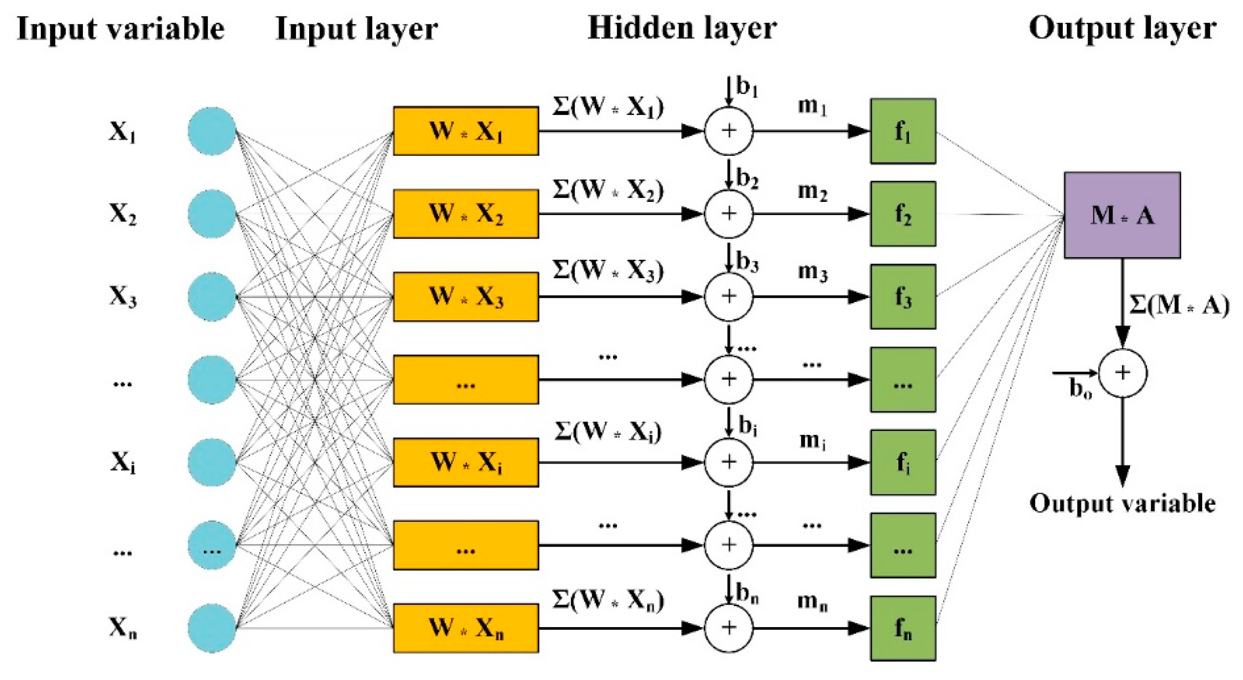
A classical feedforward ANN contains layers of nodes or neurons which have weighted connections with the nodes of the previous and preceding layers. Starting with the input layers in which each node presented for input, information or signals are propagated the subsequent layers until the information reaches the output layer. The output layer provided the predicted variable(s) and is compared with the labels of corresponding samples in the database. Figure 1 provides a typical example of the structure of ANN composed of one hidden layer.

The error of the predicted outputs and the labels is used to update the weights in the network. The weight adjustment is so-called the backpropagation and conducted each time a set of b samples (i.e., batch size) is “consumed”. This weight updating process is repeated until all samples of the train set are ingested, and an epoch is complete. The maximum number of epochs is set as the stop condition for the training process. In the end, a trained ANN model contains a set of optimized weights which provides the least error on the train set.

In work presented herein, the salient goal is developing a reliable and robust ANN model and deriving its closed-form equation to predict the 5-day biochemical oxygen demand (BOD₅). Specifically, for the estimation of BOD₅ in wastewater concerning COD, SS, TN, NH₄-N and TP, a plethora of different ANN architectures will be trained and developed. To this end, a detailed and in-depth investigation of the crucial parameters affecting the performance of ANN models, such as the number of neurons per hidden layers, activation functions, data normalization techniques and cost functions, has been conducted, and it is presented in the following sections.

3.2. Experimental Database

The primary target during a mathematical simulant’s training and development phase to predict the value of a parameter depending on several other parameters is the degree to which the proposed mathematical simulant is reliable and stable/robust. To this direction, the majority of researchers give particular attention and diligence to the computational techniques and methods that shall employ for its development, while at the same time, they do not exercise the same attention and diligence concerning the database that shall be used for the training of the ANN. The authors of the present study consider that a mathematical simulant’s reliability depends primarily on the reliability and effectiveness of the database that shall be used. We do not mean a database with a large amount of data with terms reliable and effective. Reliable and effective is considered a database with its data considered to be ‘true’ and covering statistically all the range of values capable of taking each of the parameters that infringe on each particular case studied problem.

The above has an even greater value when the database is comprised of experimental and not analytical results. In the case where the database is comprised of experimental data, its reliability is affected by a multitude of factors as follows: (a) the strict adherence to the international standards intended for the preparation of the specimens/samples and the conduct of the experimental tests-laboratory measurements; (b) the observance of the number of specimens with the same characteristics that must be checked; (c) the reliability of the experimental layout that was used; (d) the experience and specialization of the personnel that conducted the previous tests; and (e) the environmental conditions in which the aforementioned specimens were maintained as well the environmental conditions of the surroundings where the previous tests were conducted.

The observance requirement of the above rules is considered particularly imperative when the experimental database comprises experimental data produced from diverse laboratories and research groups.

According to the above principles for the training and development of a multitude of artificial neural networks and the selection among them of the best for the estimation of BOD₅ in wastewater, an experimental database was created, comprised of 387 datasets that correspond to 387 laboratory measurements that were conducted at the entrance of the sewage treatment plant located at Komotini region, Northern Greece. The samples were collected on a monthly basis from 2014–2021. Standard analytical methods were used to determine all parameters. All analytical methods were described in detail for water and wastewater experiments [41]. For each wastewater sample six water quality variables were laboratory measured. Precisely, for each sample were estimated the COD, SS, TN, NH₄-N, TP and BOD₅ concentrations. The measured values of the first five variables were used as input parameters, while the value of the sixth variable (BOD₅) as the output parameter during the training and development process of ANN models. The database is presented in Table S1 of Supplementary Materials.

Table 3. Statistical analysis of the input and output parameters used in this research for the training and development of artificial neural networks.

Variable	Symbol	Units	Category	Data Used in NN Models
				Min	Average	Max	STD	CV
Chemical Oxygen Demand	COD	mg L−1	Input	211.00	410.73	551.00	71.37	0.17
Suspended Solids	SS	mg L−1	Input	142.00	228.34	302.00	27.64	0.12
Total Nitrogen	TN	mg L−1	Input	44.20	66.44	84.25	9.17	0.14
Ammonia Nitrogen	NH4-N	mg L−1	Input	39.30	52.52	70.10	7.67	0.15
Total Phosphorous	TP	mg L−1	Input	2.96	5.86	8.65	1.17	0.20
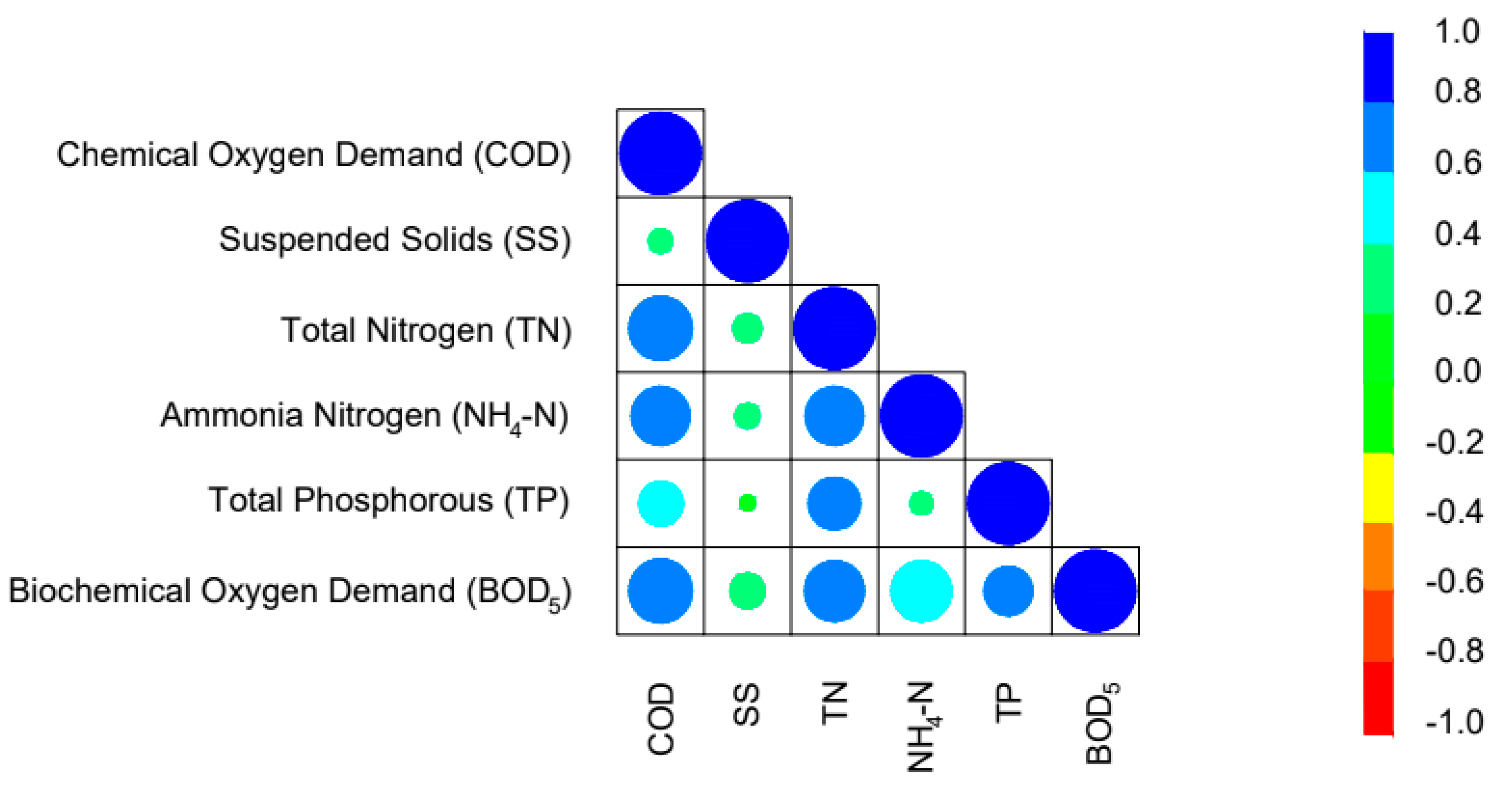
Biochemical Oxygen Demand	BOD5	mg L−1	Output	128.00	238.27	348.00	45.35	0.19

presents for each parameter the minimum, average, and maximum value as well as the standard deviation (STD) and the coefficient of variation (CV). In

Table 4. Correlation matrix of the studied input and output variables.

Variable	Symbol	COD	SS	TN	NH4-N	TP	BOD5
Chemical Oxygen Demand	COD	1.00	0.29	0.78	0.72	0.54	0.78
Suspended Solids	SS	0.29	1.00	0.35	0.30	0.18	0.43
Total Nitrogen	TN	0.78	0.35	1.00	0.72	0.64	0.74
Ammonia Nitrogen	NH4-N	0.72	0.30	0.72	1.00	0.27	0.58
Total Phosphorous	TP	0.54	0.18	0.64	0.27	1.00	0.60
Biochemical Oxygen Demand	BOD5	0.78	0.43	0.74	0.58	0.60	1.00

and Figure 2 the importance of the Pearson correlation factors between the six parameters are presented.

These values are beneficial since they indicate if there is a strong dependence of one parameter on the other. Additionally, the values of the last row of the table are indicative at the first level if there is dependence between each of the five input parameters with the output variable. It is observed that in rank, the parameters with the most significant correlation with the biochemical oxygen demand are the COD, the TN and the TP, with Pearson correlations factors 0.78, 0.74 and 0.60, respectively. In the following subsection, they will be presented thoroughly and in-depth the sensitivity analysis results of the output parameter of BOD₅ in relation with each one of the five input parameters using the Cosine Amplitude Method (CAM) [42] and the experimental database. Researchers have widely adopted CAM method to determine the effect of each input on the output [43,44,45,46].

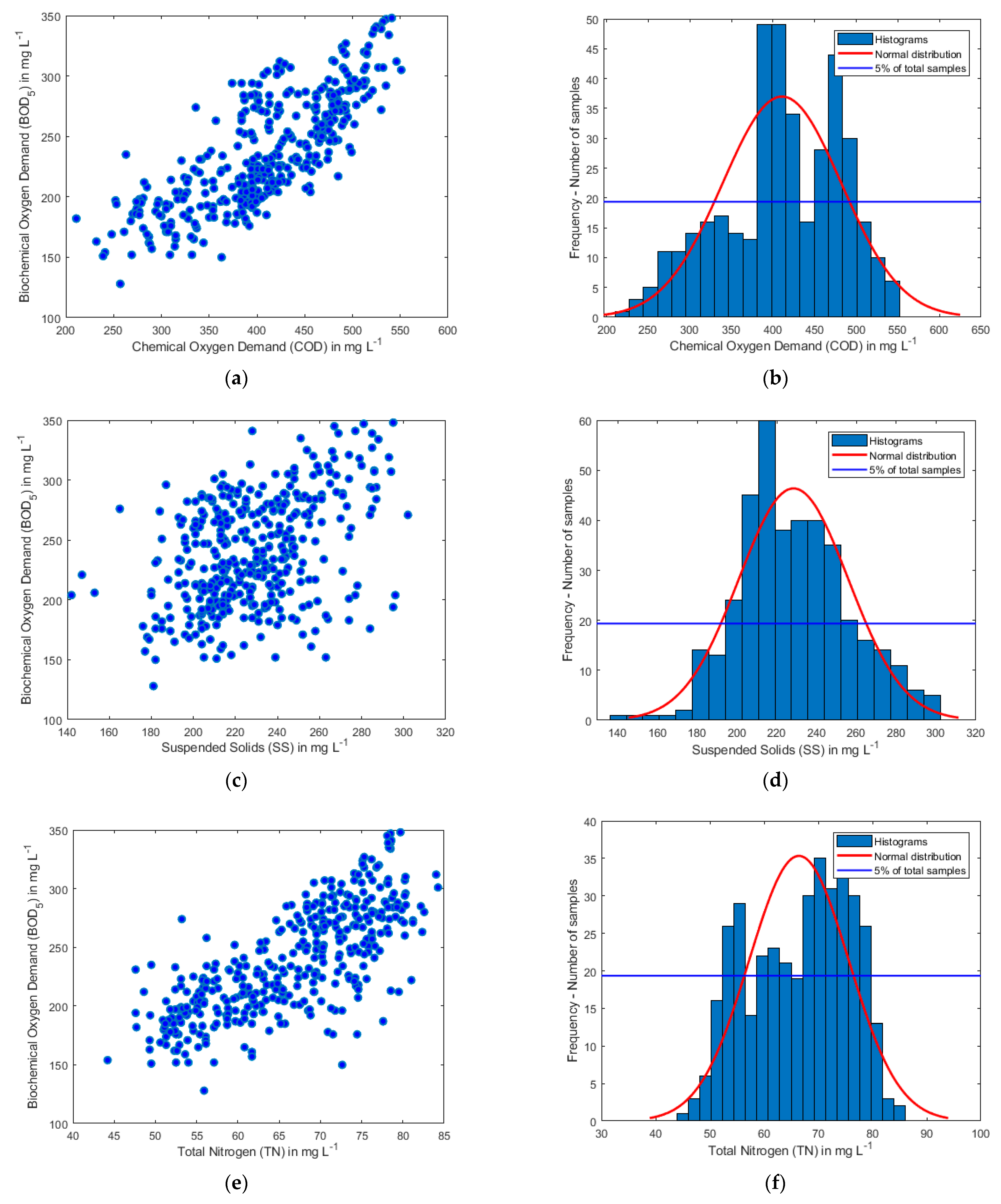
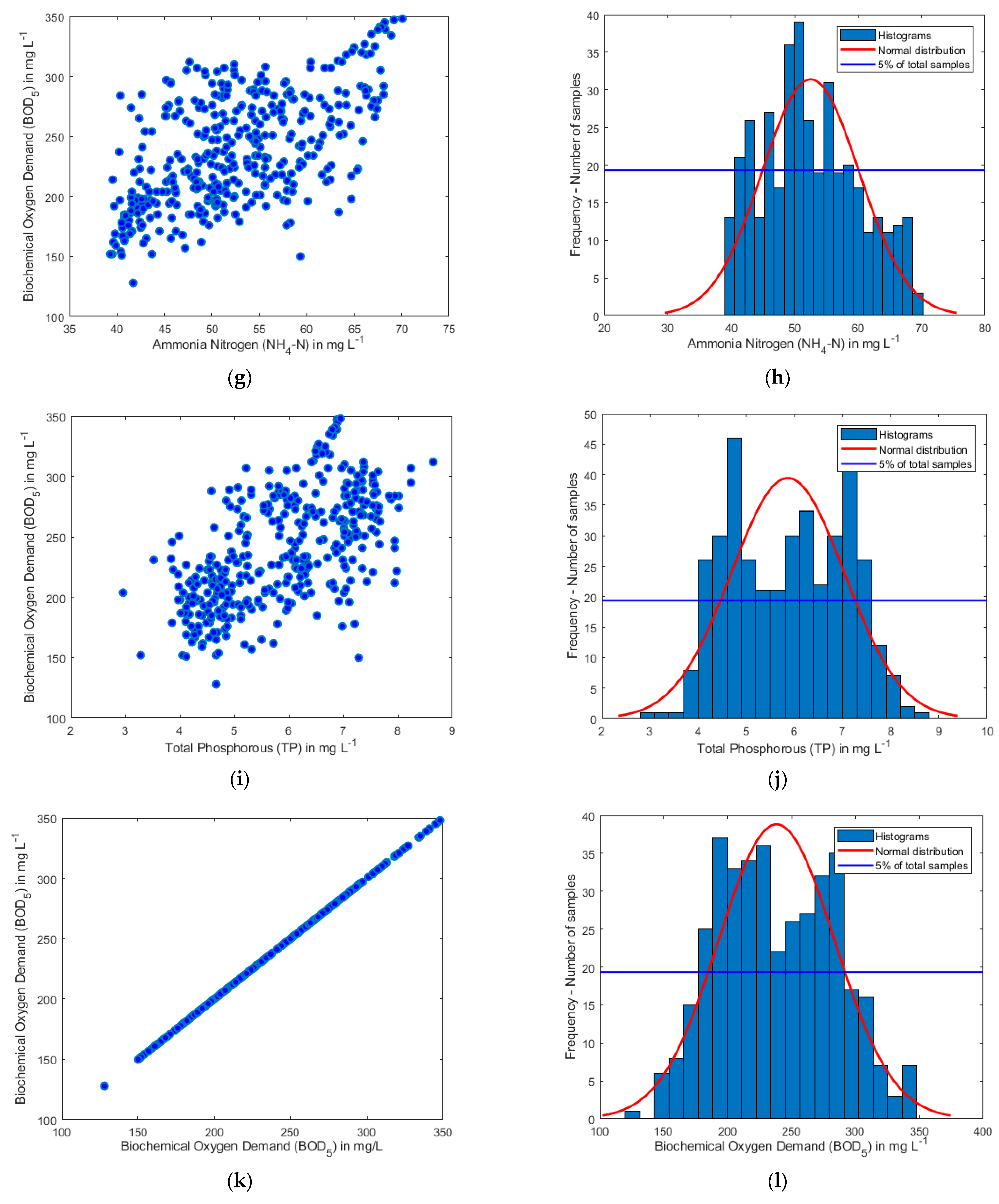
In Figure 3 the histograms are presented for each of the six variables, and graphs showing the correlation between each of the input parameters with the BOD₅.

These graphs are particularly useful since they depict for each parameter the range of values it takes and their distribution. They are beneficial since, for the ranges where we have sufficient data, the reliability of the model to be proposed shall be exceptionally high. These ranges correspond to the values of parameters for which the number of samples is greater than 5% of the dataset and are defined by the blue horizontal line in each graph. For the areas that are under the blue line, it is required to be done enrichment of the database with more data.

3.3. Sensitivity Analysis of the BOD₅ on the Input Parameters Based on the Experimental Database

During the training and development of the computational models for the prediction of the value of a parameter (output parameter) as a function of several other parameters (input parameters) that enter each case problem, it is interesting to explore the sensitivity that is exhibited by the output parameter in terms of the input parameters. This is particularly useful for it enables us to exclude a series of parameters that do not affect the estimated parameter but, at the exact moment, guides to exhibit intense attention to the parameters that significantly affect the output parameter value. The exclusion of several parameters from the current studied problem has decreased the computing time and helped to discover the problem’s nature and governing laws.

A first estimation of the dependence between the parameters and much more for the input parameters with the output parameter is given by the value of the Pearson correlation factor. Additionally, because of the subject’s great importance, they have proposed a multitude of sensitivity analysis methods with a target the as much possible estimation of the sensitivity and dependence of the output parameter from the input parameters. Between them, there is the cosine amplitude method (CAM), which has been proposed by Jong and Lee [42] and has been accepted by a multitude of researchers [35,47,48,49,50,51].

The cosine amplitude method (CAM) was used to construct a data array, X, as follows:

$$\mathrm{X}=\left\{{\mathrm{x}}_1,{\mathrm{x}}_2,{\mathrm{x}}_3,\dots ,{\mathrm{x}}_{\mathrm{i}},\dots ,{\mathrm{x}}_{\mathrm{n}}\right\}$$

(1)

where variable ${\mathrm{x}}_{\mathrm{i}}$ in array, X is a length vector of m expressed by:

$${\mathrm{x}}_{\mathrm{i}}=\left\{{\mathrm{x}}_{\mathrm{i}1},{\mathrm{x}}_{\mathrm{i}2},{\mathrm{x}}_{\mathrm{i}3},\dots ,{\mathrm{x}}_{\mathrm{im}}\right\}$$

(2)

The relationship between ${\mathrm{R}}_{\mathrm{ij}}$ (strength of the relation) and datasets of ${\mathrm{x}}_{\mathrm{i}}$ and ${\mathrm{x}}_{\mathrm{j}}$ defined by:

$${\mathrm{R}}_{\mathrm{ij}}=\frac{{{\displaystyle \sum }}_{\mathrm{k}=1}^{\mathrm{m}}{\mathrm{x}}_{\mathrm{ik}}{\mathrm{x}}_{\mathrm{jk}}}{\sqrt{{{\displaystyle \sum }}_{\mathrm{k}=1}^{\mathrm{m}}{\mathrm{x}}^2{}_{\mathrm{ik}}{{\displaystyle \sum }}_{\mathrm{k}=1}^{\mathrm{m}}{\mathrm{x}}^2{}_{\mathrm{ik}}}}$$

(3)

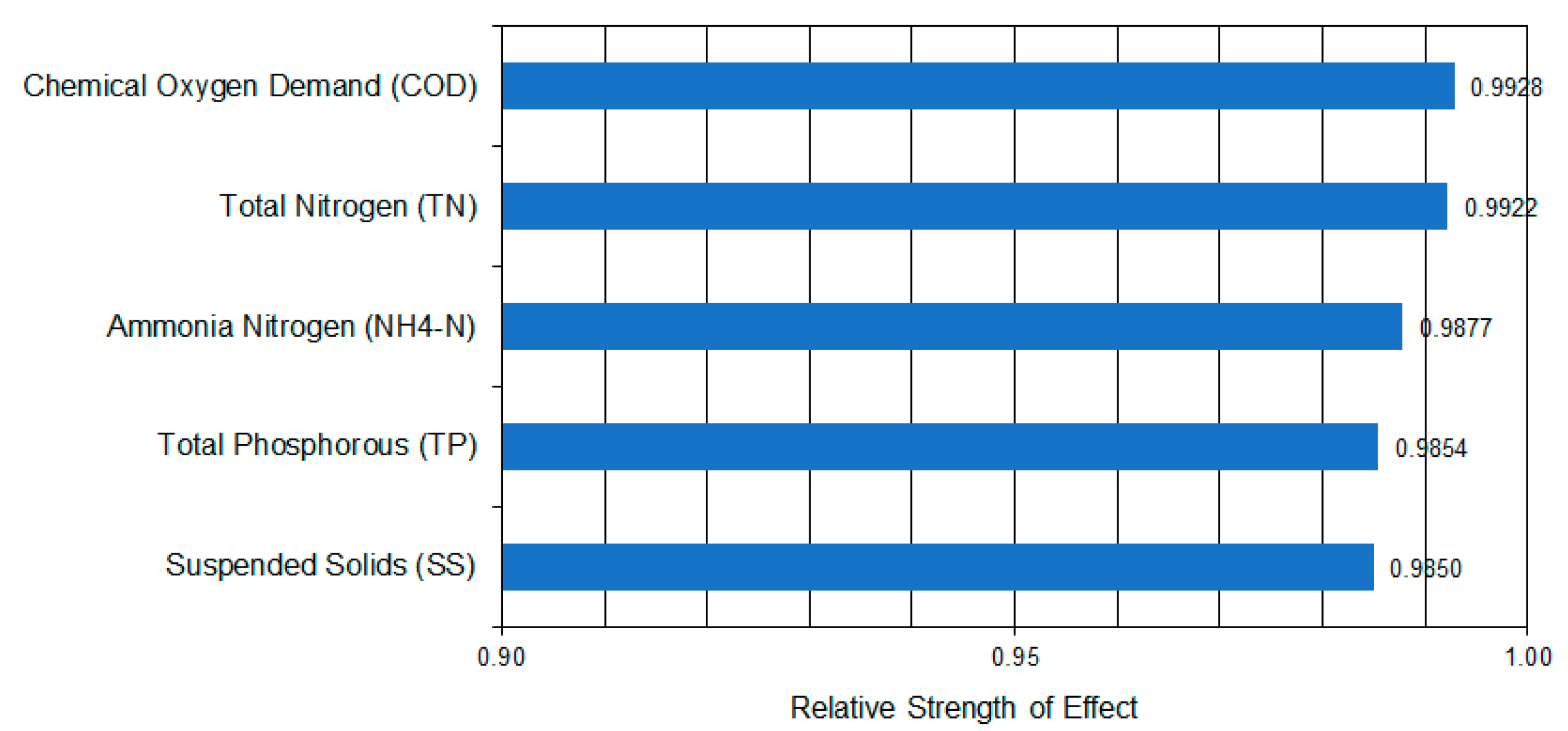
The result of the sensitivity analysis, based on the datasets of the experimental database used in the present work, is presented in Figure 4. It depicted that from the five input parameters, the COD and TN had the strongest influence on the BOD₅ (Figure 4). This finding fully agrees with Pearson correlation factors presented in the preview’s subsection. Furthermore, it is worth noting that all the input parameters can be characterized as crucial since they have also strongly related to BOD₅, achieving values greater than 0.98.

3.4. Performance Indexes

The predictive accuracy of the developed neural network models was assessed using the root mean square error (RMSE), the mean absolute percentage error (MAPE), and the Correlation Coefficient (R²) [49,51,52,53,54,55].

$$RMSE=\sqrt{\frac{1}{n}{\displaystyle \sum }_{i=1}^n{\left(x_i-y_i\right)}^2}$$

(4)

$$MAPE=\frac{1}{n}{\displaystyle \sum }_{i=1}^n\left|\frac{x_i-y_i}{x_i}\right|$$

(5)

$$R^2=1-\left(\frac{{{\displaystyle \sum }}_{i=1}^n{\left(x_i-y_i\right)}^2}{{{\displaystyle \sum }}_{i=1}^n{\left(x_i-\overline{x}\right)}^2}\right)$$

(6)

where $n$ denotes the total number of datasets, and $x_i$ and $y_i$ represent the predicted and target values, respectively.

Recent research has highlighted the limitations of the root mean square error (RMSE), the mean absolute percentage error (MAPE), and the Correlation Coefficient (R²) to assess the predictive accuracy of models [30,53]. The comparison of the performance of mathematical using the Pearson correlation factor is considered precarious given that except the comparison of the values of R or R² it is also required the comparison of the inclination angle of the line. Such a case is when a mathematical simulant always predicts a constant value regardless of the input parameters values. In this case, the value of R = 1.00 while the inclination angle is equal to zero.

To this end, the a20-index, has been recently proposed [43,56,57,58,59,60,61,62] for assessing the reliability of neural networks:

$$\mathrm{a}20-\mathrm{index}=\frac{\mathrm{m}20}{\mathrm{M}}$$

(7)

where M denotes the number of dataset samples and m20 denotes the number of samples with a ratio of the true value to the estimated-predicted value between 0.80 and 1.20. In an ideal forecasting model, the value of a20-index is equal to 1.00. The proposed a20-index is a simple statistical index having the advantage to include a physical engineering meaning, as it reveals the number of experiments that satisfy the predicted values with a 20% deviation from the ‘true’ values.

At this point it is worth stressing the very large significance of the database that shall be used for the training and development of the soft computing-based forecasting models. A comparison using different performance indices must be referring to an adequate number of data and indeed to be reliable must be based on the same database.

4. Results and Discussion

4.1. Development of ANN Models

Several hyperparameters and neural network structure/architecture must be determined ahead of time in the context of the training and development ANN models. This provides the benefit of developing an ANN model that is exceptionally optimized for the problem under investigation. However, unless a certain level of expertise is available, selecting appropriate values for these parameters and appropriate neuron layouts can be intimidating. In other words, the “human in the loop” concept is thought to be critical for tuning an efficient ANN model. Furthermore, special care about the overfitting problems should be paid. The selection of the optimum model among the plethora of training and developed soft computing models should be based not only on statistical indices but also on the derivation of curves which should be smooth revealing the nature of the problem under investigation.

However, in this study, the optimal ANN structure is not selected based on expertise or intuition. However, it is derived from an optimization procedure that trains and tests ANNs using a plethora of alternative hyper parameter combinations and ranks them according to predefined performance indices as well as it mentioned above taking care whether overfitting of the data taking place. Except for the fixed number of hidden layers, the optimization procedure combines the following parameters: (a) data normalization; (b) the number of neurons in the hidden layer; (c) cost function; and (d) activation function.

Table 5. Hyperparameters for the training and development of ANN models applied in this study.

Parameter	Value	Matlab Function(s)
Training Algorithm	Levenberg-Marquardt Algorithm	trainlm
Normalization	Without any normalization Minmax in the range [0.10–0.90], [0.00–1.00] and [−1.00–1.00] Zscore	Mapminmax zscore
Number of Hidden Layers	1
Number of Neurons per Hidden Layer	1 to 50 by step 1
Control random number generation	10 different random generation	rand(seed, generator), where the generator range from 1 to 10 by step 1
Training Goal	0
Epochs	200
Cost Function	Mean Square Error (MSE) Sum Square Error (SSE)	mse sse
Transfer Functions	Hyperbolic Tangent Sigmoid transfer function (HTS) Log-sigmoid transfer function (LS) Linear transfer function (Li) Positive linear transfer function (PLi) Symmetric saturating linear transfer function (SSL) Soft max transfer function (SM) Competitive transfer function (Co) Triangular basis transfer function (TB) Radial basis transfer function (RB) Normalized radial basis transfer function (NRB) Hard-limit transfer function (HL) Symmetric hard-limit transfer function (SHL)	tansig logsig purelin poslin satlins softmax compet tribas radbas radbasn hardlim hardlims

shows the alternative options for these parameters, as well as some predetermined configuration options. Twelve different activation functions are investigated, including the common Hyperbolic Tangent Sigmoid (HTS), Log-sigmoid (LS), and Linear (Li) functions. If all other parameters are held constant, this results in 144 (12 × 12) alternative combinations to be trained and tested. Regarding the used cost functions, the MSE and SSE functions are investigated, whereas four data normalization techniques are applied on the input and output parameters, including no normalization at all. Considering the varying random number generator, all of these alternative ANN configuration parameters resulted in 576.000 different ANN models under evaluation (i.e., 50 × 10 × 42 × 4 × 10) (10 alternatives). At this point, it should be pointed out that the Levenberg–Marquardt algorithm (LM) has been applied during training process of ANN mathematical models.

The training of the 576.000 alternative ANN architectures did not use the entire dataset of 387 samples. The dataset was divided into three sub-datasets to evaluate the generality of the developed ANN model: the first dataset included 66.7% of the entire database (258 specimens) and was used for training the ANN architectures, the second dataset included 16.8% of the entire database (65 specimens) and was used for testing the ANN architectures, and the third dataset included the remaining 16.5% of the entire sample (64 specimens). The three datasets are referred to as “training datasets”, “testing datasets”, and “validation datasets”, in that order. To eliminate potential bias, the sample was randomly divided into three datasets using a programmatic procedure.

Table 6. Architectures and hyperparameters of the top twenty developed ANN LM models based RMSE index and testing phase.

Ranking	Normalization Technique	Cost Function	Transfer Function		Architecture	Datasets Performance Indices
			Input Layer	Output Layer		Testing		Training		All
						R	RMSE	R	RMSE	R	RMSE
1	Minmax [−1.00, 1.00]	MSE	logsig	satlins	5-8-1	0.9443	16.8563	0.9208	17.6044	0.9217	17.6065
2	Minmax [0.10, 0.90]	MSE	poslin	satlins	5-29-1	0.9421	17.8418	0.9057	19.1355	0.9110	18.7234
3	Minmax [−1.00, 1.00]	SSE	tribas	tansig	5-14-1	0.9407	17.7982	0.9319	16.3818	0.9287	16.8636
4	Minmax [0.10, 0.90]	MSE	tansig	purelin	5-13-1	0.9406	17.5336	0.9238	17.2764	0.9214	17.6425
5	Minmax [0.10, 0.90]	MSE	softmax	radbas	5-17-1	0.9400	17.7336	0.9156	18.1454	0.9164	18.2035
6	Minmax [−1.00, 1.00]	MSE	tansig	purelin	5-11-1	0.9400	17.5935	0.9298	16.6148	0.9224	17.5536
7	Minmax [0.10, 0.90]	MSE	logsig	satlins	5-8-1	0.9399	17.5855	0.9161	18.1001	0.9179	18.0053
8	Minmax [0.10, 0.90]	SSE	softmax	logsig	5-29-1	0.9396	17.7540	0.9311	16.4914	0.9275	17.0689
9	Minmax [0.10, 0.90]	SSE	satlins	purelin	5-15-1	0.9394	18.6357	0.9012	19.6172	0.9066	19.3523
10	Minmax [0.00, 1.00]	MSE	logsig	satlins	5-5-1	0.9393	18.7060	0.9136	18.4874	0.9150	18.5984
11	Minmax [0.10, 0.90]	SSE	softmax	satlins	5-26-1	0.9393	18.1376	0.9077	18.9646	0.9116	18.7815
12	Minmax [0.00, 1.00]	MSE	softmax	purelin	5-41-1	0.9388	17.8211	0.9217	17.5291	0.9215	17.7143
13	Minmax [0.10, 0.90]	MSE	tansig	purelin	5-8-1	0.9388	17.6942	0.9160	18.1425	0.9179	17.9936
14	Minmax [0.10, 0.90]	MSE	softmax	radbas	5-23-1	0.9388	19.0606	0.9135	18.4091	0.9155	18.4651
15	Minmax [0.10, 0.90]	MSE	logsig	logsig	5-12-1	0.9387	16.7798	0.9320	16.3995	0.9282	16.8627
16	Minmax [0.00, 1.00]	MSE	softmax	purelin	5-22-1	0.9387	18.2816	0.9105	18.6790	0.9125	18.6410
17	Minmax [0.00, 1.00]	MSE	softmax	poslin	5-22-1	0.9387	18.2816	0.9105	18.6790	0.9125	18.6410
18	Minmax [0.00, 1.00]	MSE	tansig	satlins	5-6-1	0.9386	17.5546	0.9164	18.0637	0.9166	18.1632
19	Zscore	MSE	poslin	purelin	5-9-1	0.9385	18.1809	0.9076	18.9472	0.9105	18.7648
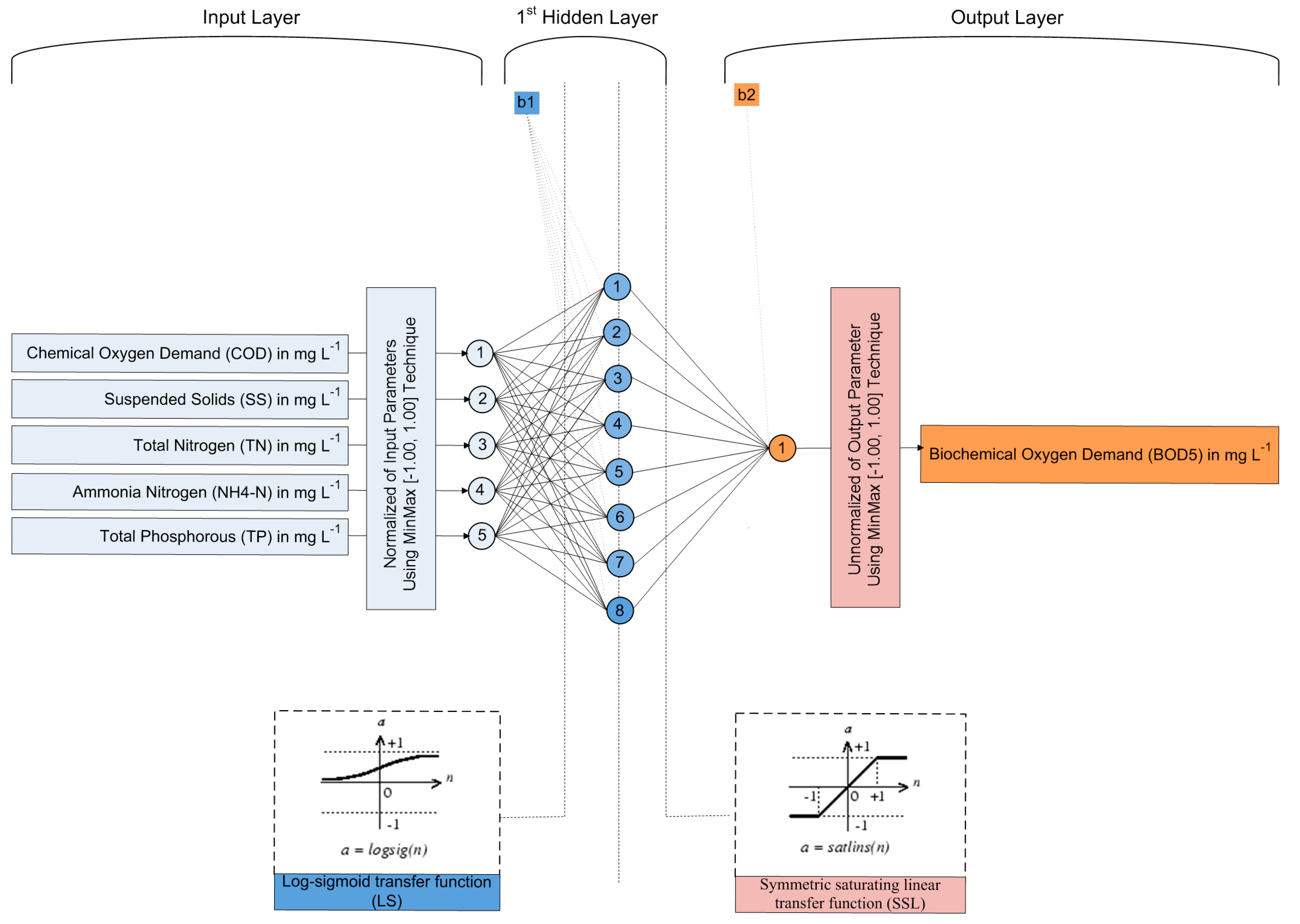
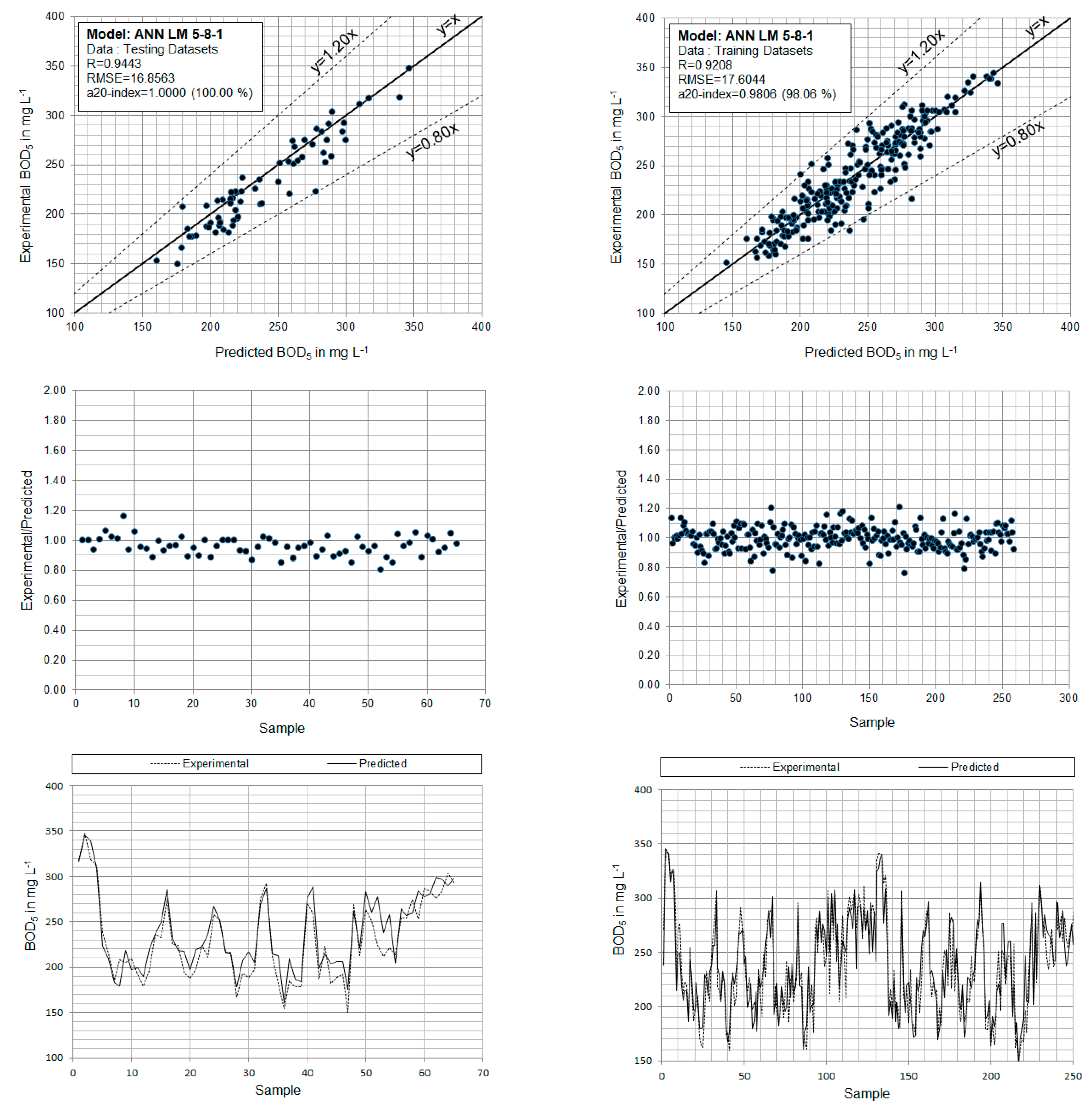
20	Minmax [0.00, 1.00]	SSE	tansig	purelin	5-7-1	0.9384	17.1610	0.9100	18.7052	0.9110	18.7294

tabulates the top twenty ANN architectures based on their achieved values of RMSE index and for the case of testing datasets and configuration parameters. The first, which is preferred as the best and is regarded to as ANN LM 5-8-1 (the numbers refer to the five (5) input parameters, the eight (8) neurons in the hidden layer and the one (1) output parameter which is the BOD₅), achieves the best overall performance metrics, both in terms of RMSE (16.8563) and R (0.9443). The best ANN LM 5-8-1 model utilizes the MinMax function for data normalization, which converts input and output values between [−1.00, 1.00]. It also applies as activation functions the Log-Sigmoid function (LS) for the input layer and the Symmetric saturating linear function (SSL) for the output layer, with the MSE function as its cost function. Figure 5 exhibits the neuron layout and overall architecture of the best ANN LM 5-8-1 model.

Table 7. Summary of prediction capability of the optimum ANN LM 5-8-1 model.

Model	Datasets	Performance Indices
		a20-Index	R	RMSE	MAPE	VAF
ANN LM 5-8-1	Training	0.9806	0.9208	17.6044	0.0582	84.7803
	Test	1	0.9443	16.8563	0.0571	89.1499

displays detailed and in-depth achieved performance indices for both training and testing datasets of the best ANN LM 5-8-1 model. Its performance on training datasets is expected to improve, particularly in the a20-index, where it matches over 98% of the samples within a 20 percent margin. The same index is 100.00% when compared to the testing datasets, which is an excellent value. At this point should be noted that the better achieved indices for testing datasets compared to training datasets clearly depict that not overfitting problems is taken place. To the authors best knowledge, the achieved performance is the better than any other performance reported in the related topic.

Furthermore, values for the training and testing datasets are presented in Figure 6 as scatter plots of the ‘true’ vs. predicted by the best ANN LM 5-8-1 model. Except for the diagonal line (ideal prediction), two more dotted lines are drawn in these diagrams, indicating a ±20% error. Furthermore, Figure 6 is a more useful figure depicts the ratio of ‘true’ values to predicted values of BOD₅ in wastewater both for training and testing datasets.

4.2. Closed-Form Equation for the Estimation of BOD₅ in Wastewater

As presented in the previous section, the ANN LM 5-8-1 model is the best among the many different trained and developed architectures. That is the best is documented that this model has optimal values for the performance indices used for ranking other ANN models. It is worth noting that this is a standard procedure for the multitude of scientific publications.

At this point, the authors consider it necessary to state clearly that such a procedure is not safe and reliable because it is impossible to test the reliability-validity of these values. Additionally, the results of such a research work are not immediately applicable to the scientists of this discipline and much more to the engineers in practice.

Intending to treat the above weaknesses, the authors consider it necessary to present the architecture corresponding to the best ANN model and the final values of weights and biases to make the design of the mathematical simulant possible. Giving the mathematical equation that describes the best mathematical simulant would be more beneficial. Under the prism of all the above in the present section, the derived equation for the prediction of both normalized and absolute values of BOD₅, using COD, SS, TN, NH₄-N and TP are expressed by the following equation for the optimum developed ANN LM 5-8-1 model:

$$BOD{5}_{norm}= \mathrm{satlins}\left(\left[\mathrm{LW}\left\{2,1\right\}\right]\times \left[\mathrm{logsig}\left(\left[\mathrm{IW}\left\{1,1\right\}\right]\times \left[\mathrm{IP}\right]+\left[\mathrm{B}\left\{1,1\right\}\right]\right)\right]+\left[\mathrm{B}\left\{2,1\right\}\right]\right)$$

(8)

$$BOD{5}_{real}=\frac{\left(BOD{5}_{norm}-\mathrm{a}\right)\times \left(BOD{5}_{max}-BOD{5}_{min}\right)}{\mathrm{b}-\mathrm{a}}+BOD{5}_{min}$$

(9)

where a = −1.00 and b = 1.00 are the lower and upper limits of the minmax normalization technique applied on the data, $\mathit{B}\mathit{O}\mathit{D}{\mathbf{5}}_{\mathit{m}\mathit{a}\mathit{x}}$ = 348 and $\mathit{B}\mathit{O}\mathit{D}{\mathbf{5}}_{\mathit{m}\mathit{i}\mathit{n}}$ = 128 are the maximum and minimum values of BOD₅ present in the database used for training and developing ANN models. The satlins and logsig are the symmetric saturating linear transfer function (SSL) and the Log-sigmoid transfer function (LS), respectively, as discussed. Their details (equations and graphs) are presented in detail in

Table A1. Transfer functions.

SN	Transfer Function/Equation/Matlab Function	Graph
1	The symmetric saturating linear transfer function (SSL)
	$a=f\left(n\right)=\{\begin{array}{c}-1, \\ \begin{array}{c}n, \\ -1, \end{array}\end{array}\begin{array}{c} n\le -1\\ \begin{array}{c}-1<n<1\\ n\ge 1\end{array}\end{array}$
	$a=f\left(n\right)=\mathrm{satlins} \left(n\right)$
2	The log-sigmoid transfer function (LS)
	$a=\frac{1}{1+\exp \left(-n\right)}$
	$\mathrm{a}=f\left(n\right)=\mathrm{logsig}\left(\mathrm{n}\right)$

of the Appendix A.

Equation (9) describes the developed ANN LM 5-8-1 model in a purely mathematical form so that its reproduction becomes straightforward. In Equation (8), $\left[IW\left\{1,1\right\}\right]$ is a 8$\times$5 matrix that contains the weights of the hidden layer; $\left[LW\left\{2,1\right\}\right]$ is a 1$\times$8 vector with the weights of the output layer; $\left[IP\right]$ is a 5 × 1 vector with the five (5) input variables; $\left[B\left\{1,1\right\}\right]$ is a 8$\times$1 vector that contains the bias values of the hidden layer; and $\left[B\left\{2,1\right\}\right]$ is a 1$\times$1 vector with the bias of the output layer. The $\left[IP\right]$ vector contains the five (5) normalized values of the input variables (COD, SS, TN, NH₄-N and TP). It is expressed as:

$$\left[\mathrm{IP}\right]=\left[\begin{array}{c}\mathrm{a}+\left(\mathrm{b}-\mathrm{a}\right)\left(\frac{\mathrm{COD}-\min \left(\mathrm{COD}\right)}{\max \left(\mathrm{COD}\right)-\min \left(\mathrm{COD}\right)}\right)\\ \mathrm{a}+\left(\mathrm{b}-\mathrm{a}\right)\left(\frac{\mathrm{SS}-\min \left(\mathrm{SS}\right)}{\max \left(\mathrm{SS}\right)-\min \left(\mathrm{SS}\right)}\right)\\ \mathrm{a}+\left(\mathrm{b}-\mathrm{a}\right)\left(\frac{\mathrm{TN}-\min \left(\mathrm{TN}\right)}{\max \left(\mathrm{TN}\right)-\min \left(\mathrm{TN}\right)}\right)\\ \mathrm{a}+\left(\mathrm{b}-\mathrm{a}\right)\left(\frac{{\mathrm{NH}}_4-\mathrm{N}-\min \left({\mathrm{NH}}_4-\mathrm{N}\right)}{\max \left({\mathrm{NH}}_4-\mathrm{N}\right)-\min \left({\mathrm{NH}}_4-\mathrm{N}\right)}\right)\\ \mathrm{a}+\left(\mathrm{b}-\mathrm{a}\right)\left(\frac{\mathrm{TP}-\min \left(\mathrm{TP}\right)}{\max \left(\mathrm{TP}\right)-\min \left(\mathrm{TP}\right)}\right)\end{array}\right]$$

(10)

where the $min\left(COD\right)$ = 211, $max\left(COD\right)$ = 551; $min\left(SS\right)$ = 142, $max\left(SS\right)$ = 302; $min\left(TN\right)$ = 44.20, $max\left(TN\right)$ = 84.25; $min\left(N{H}_4-N\right)$ = 39.30, $max\left(N{H}_4-N\right)$ = 70.10 and $min\left(TP\right)$ = 2.96, $max\left(TP\right)$ = 8.65 are the input parameters minimum and maximum values (shown in Table 3). The values of final weights and biases that determine the matrices $\left[IW\left\{\mathbf{1},\mathbf{1}\right\}\right]$, $\left[LW\left\{\mathbf{2},\mathbf{1}\right\}\right]$, $\left[B\left\{\mathbf{1},\mathbf{1}\right\}\right]$ and $\left[B\left\{\mathbf{2},\mathbf{1}\right\}\right]$ are presented in

Table 8. Finalized weights and bias of the optimum ANN-LM 5-8-1 model.

IW{1,1}					${\left[\mathsf{L}\mathsf{W}\left\{2,1\right\}\right]}^{\mathit{T}}$	$\left[\mathsf{B}\left\{1,1\right\}\right]$	$\left[\mathsf{B}\left\{2,1\right\}\right]$
(8 × 3)					(1 × 8)	(8 × 1)	(1 × 1)
3.8747	−3.3026	0.8841	9.8281	−1.9581	2.9497	9.6809	−0.4917
−3.8650	3.1701	0.9485	−1.1494	1.9099	−2.6746	2.1566
1.2295	−2.3973	−1.2553	2.7258	−2.3405	−2.3231	1.0974
−4.6036	3.7836	0.8690	−4.0565	7.1579	−1.1579	−1.3150
−3.0096	3.4372	0.3911	−0.1472	2.3667	2.2639	2.2077
−1.0593	−4.5452	1.0995	−4.5926	−1.9055	−0.6063	6.0657
−4.7120	3.0951	−2.9974	−9.7771	2.9426	2.6242	−10.6922
1.6124	−9.0346	0.1278	3.6006	8.0047	0.3364	7.7832

Note: $\left[IW\left\{1,1\right\}\right]$ is the matrix of weight values between the input layer and the first hidden Layer; $\left[LW\left\{\mathbf{2},\mathbf{1}\right\}\right]$ is the matrix of weight values between the 1st hidden layer and the output layer; $\left[B\left\{\mathbf{1},\mathbf{1}\right\}\right]$ is the matrix of bias values for hidden layer, and $\left[B\left\{\mathbf{2},\mathbf{1}\right\}\right]$ is the matrix of bias values for the output layer.

.

In this form of matrix multiplication, the prediction equation Equation (9) can be easily programmed in an Excel spreadsheet, and therefore it can be more easily evaluated and used in practice. It is worth noting that such an implementation can be used by various interested parties (i.e., researchers, students, engineers) without placing heavy requirements on effort and time.

4.3. Mapping of BOD₅

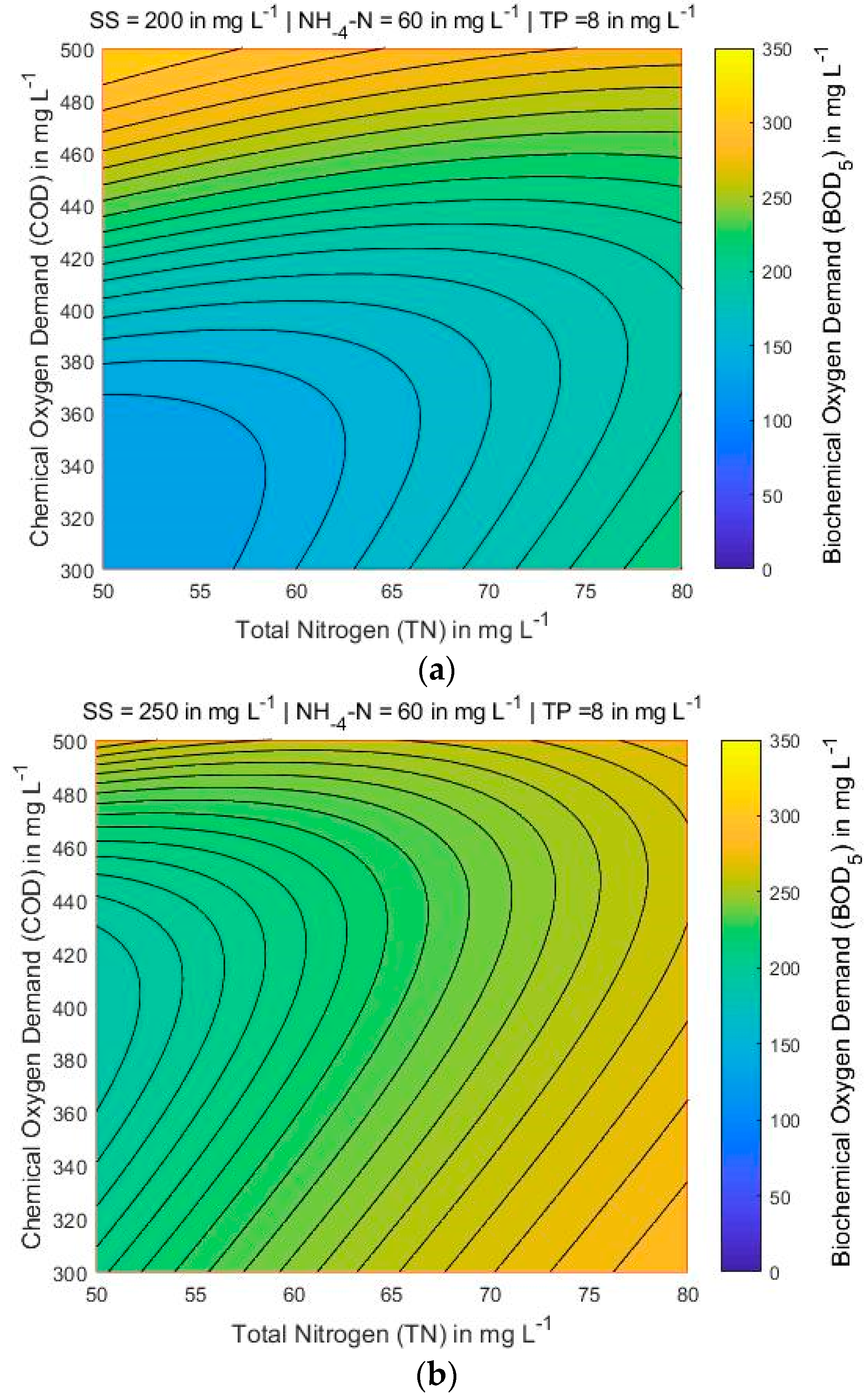
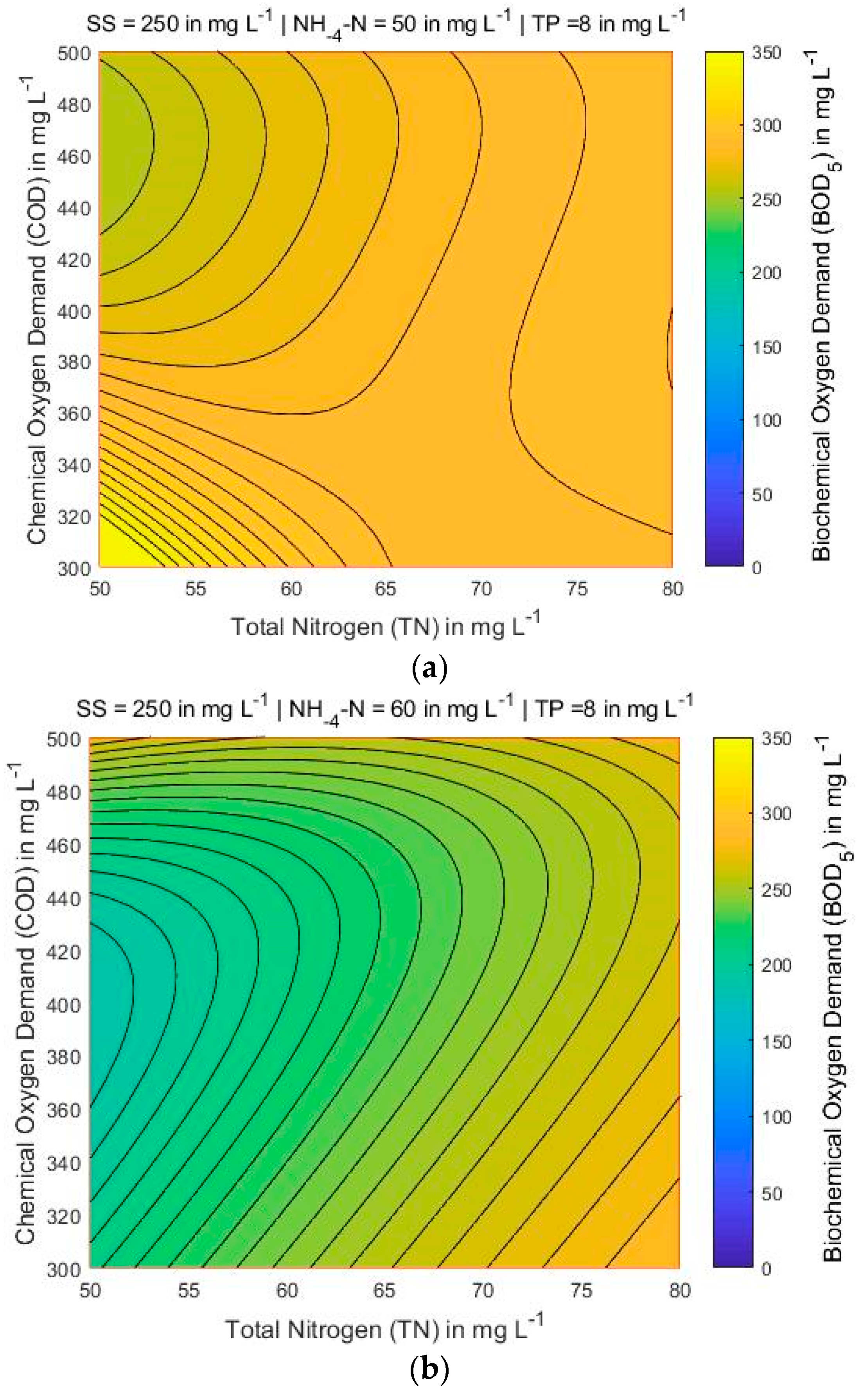
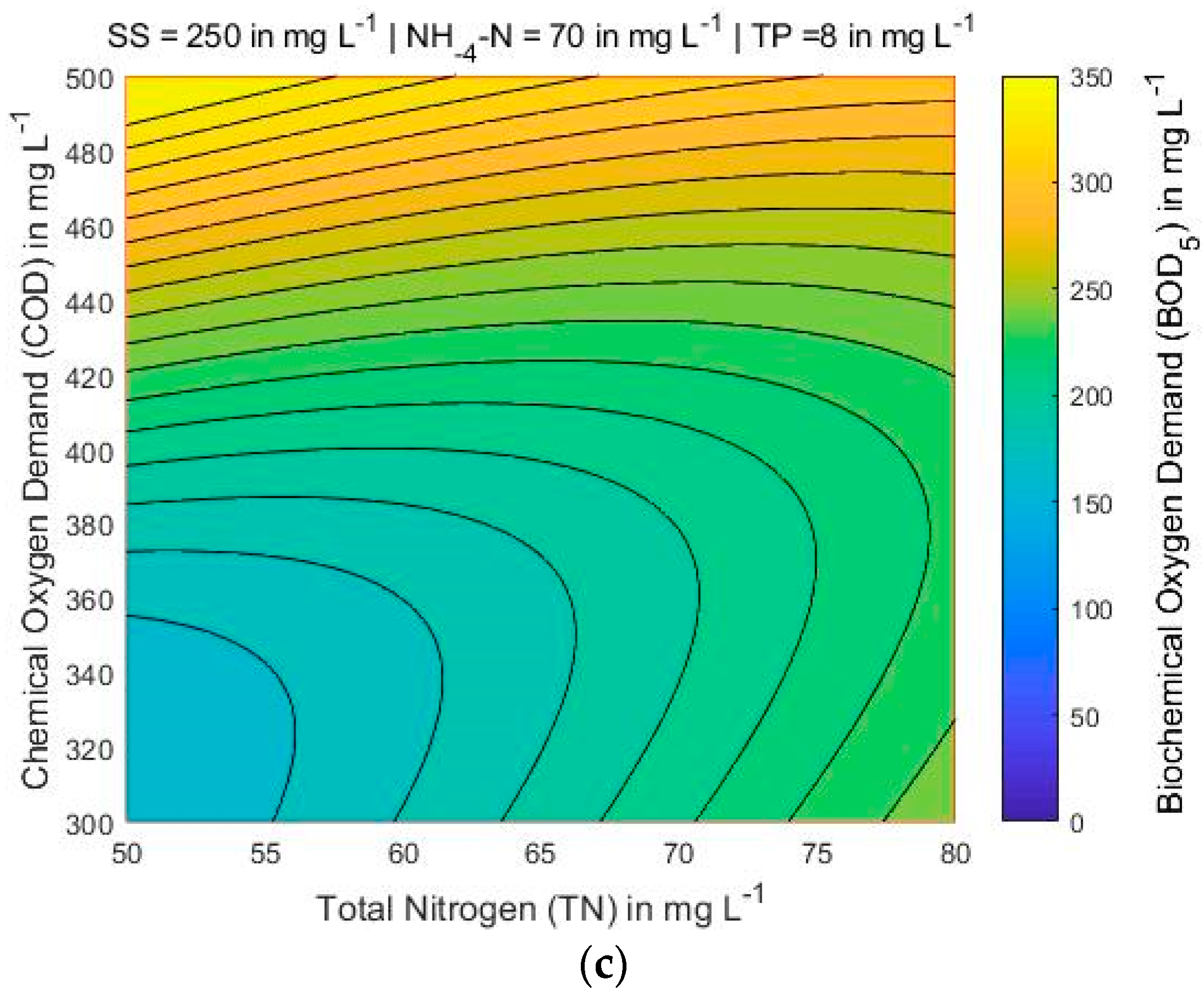
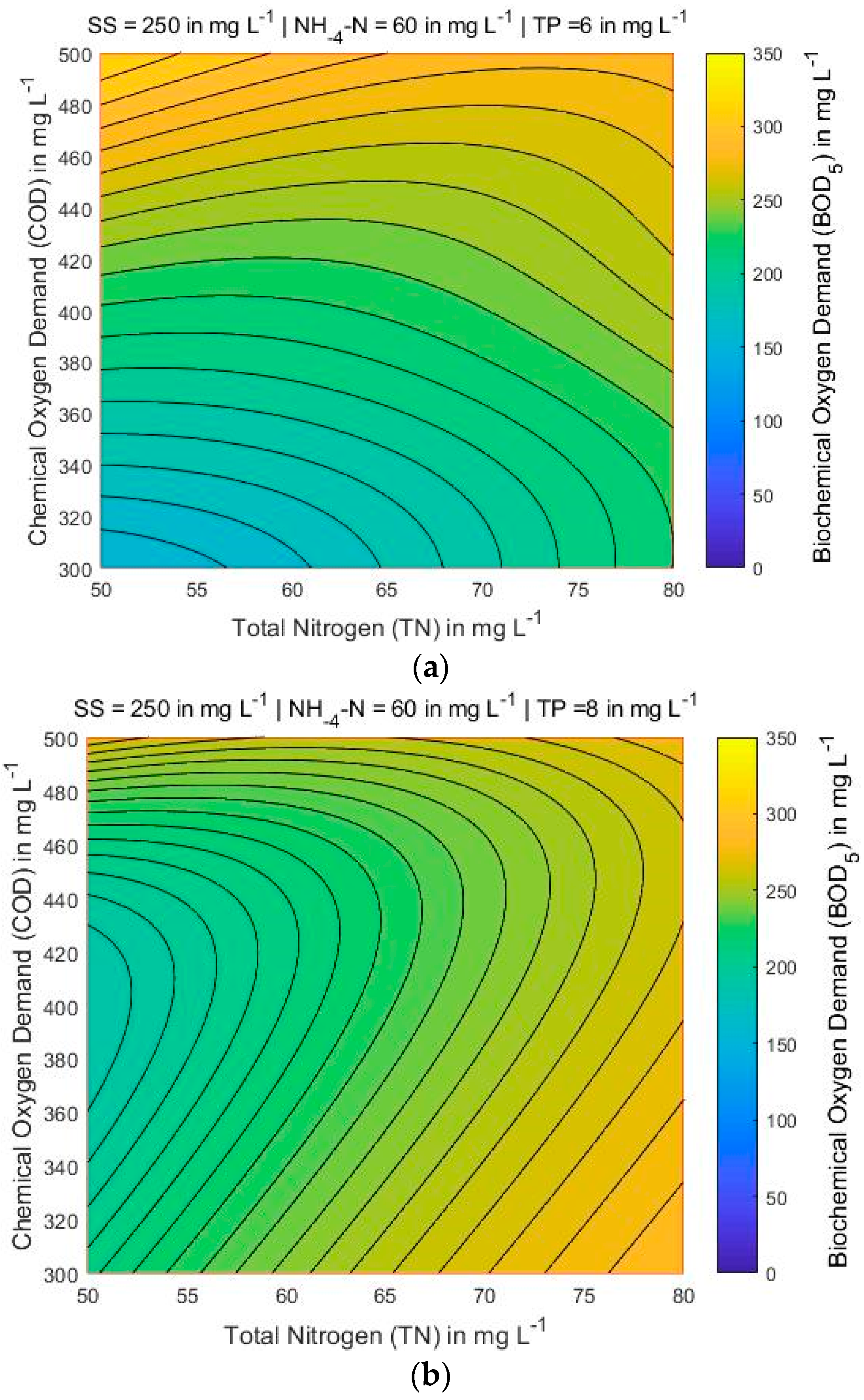
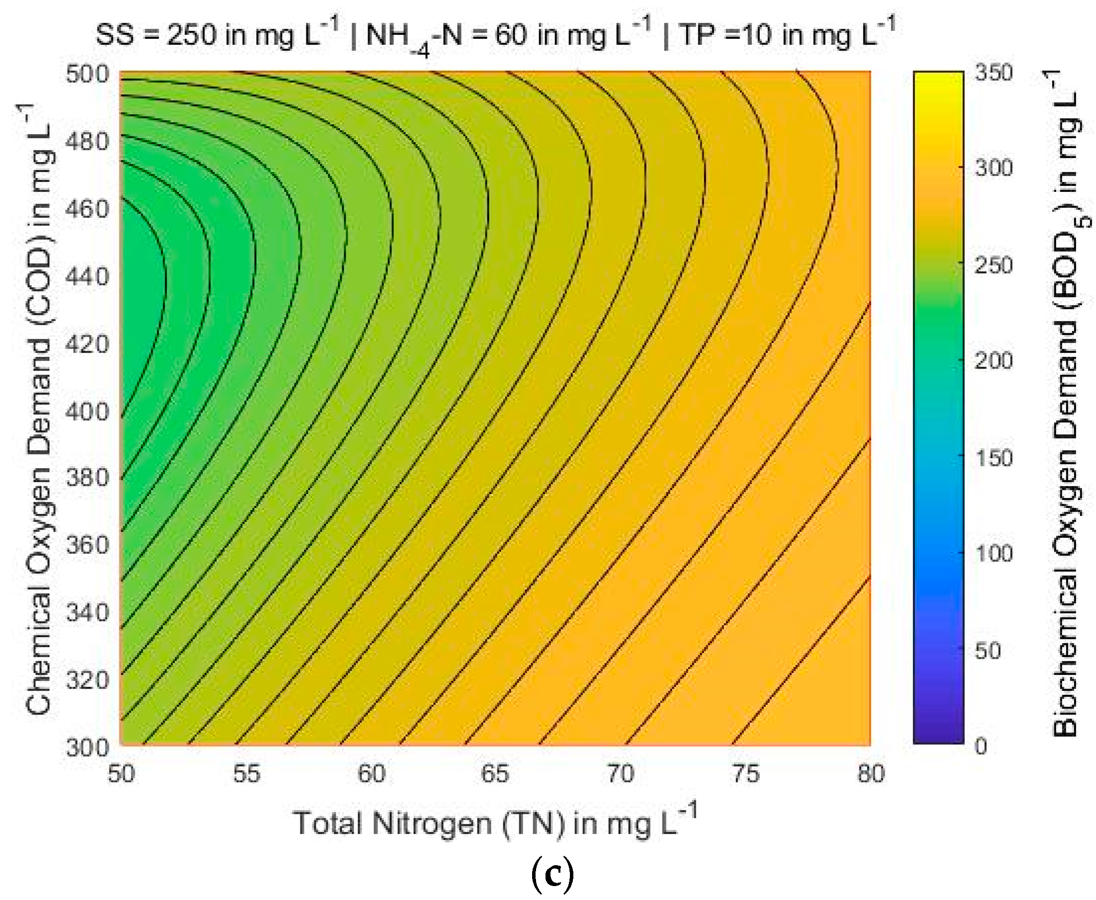
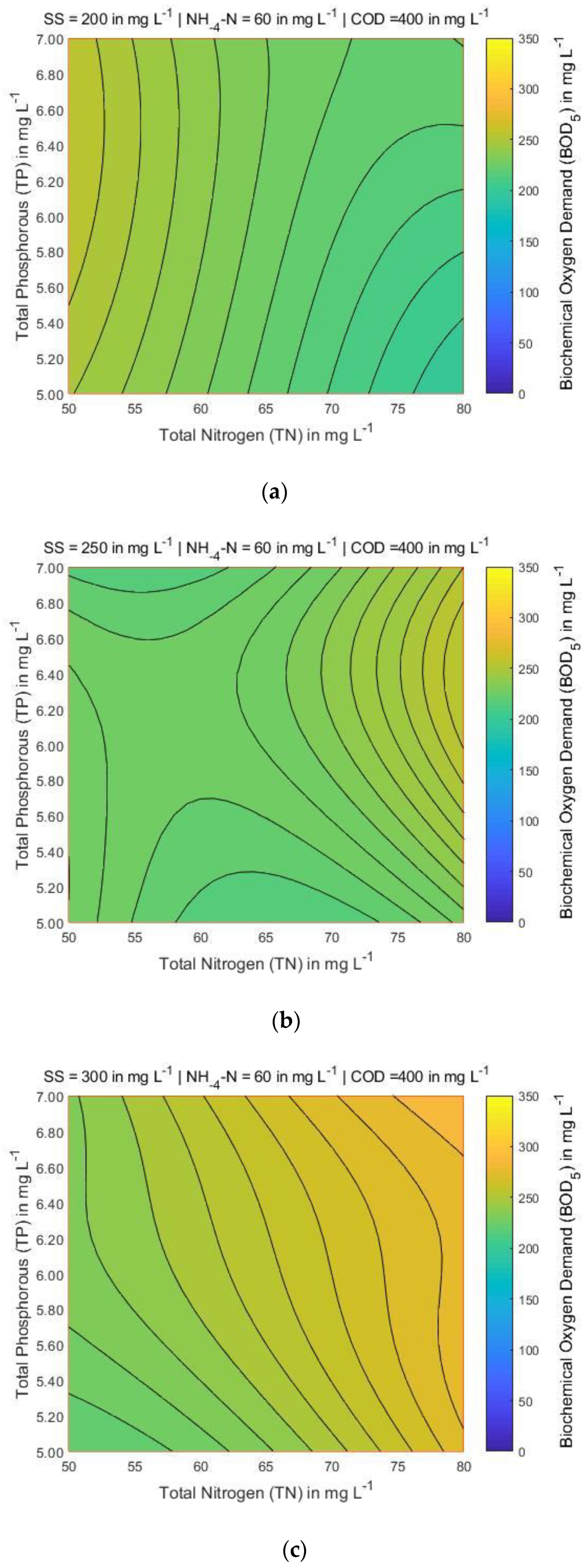
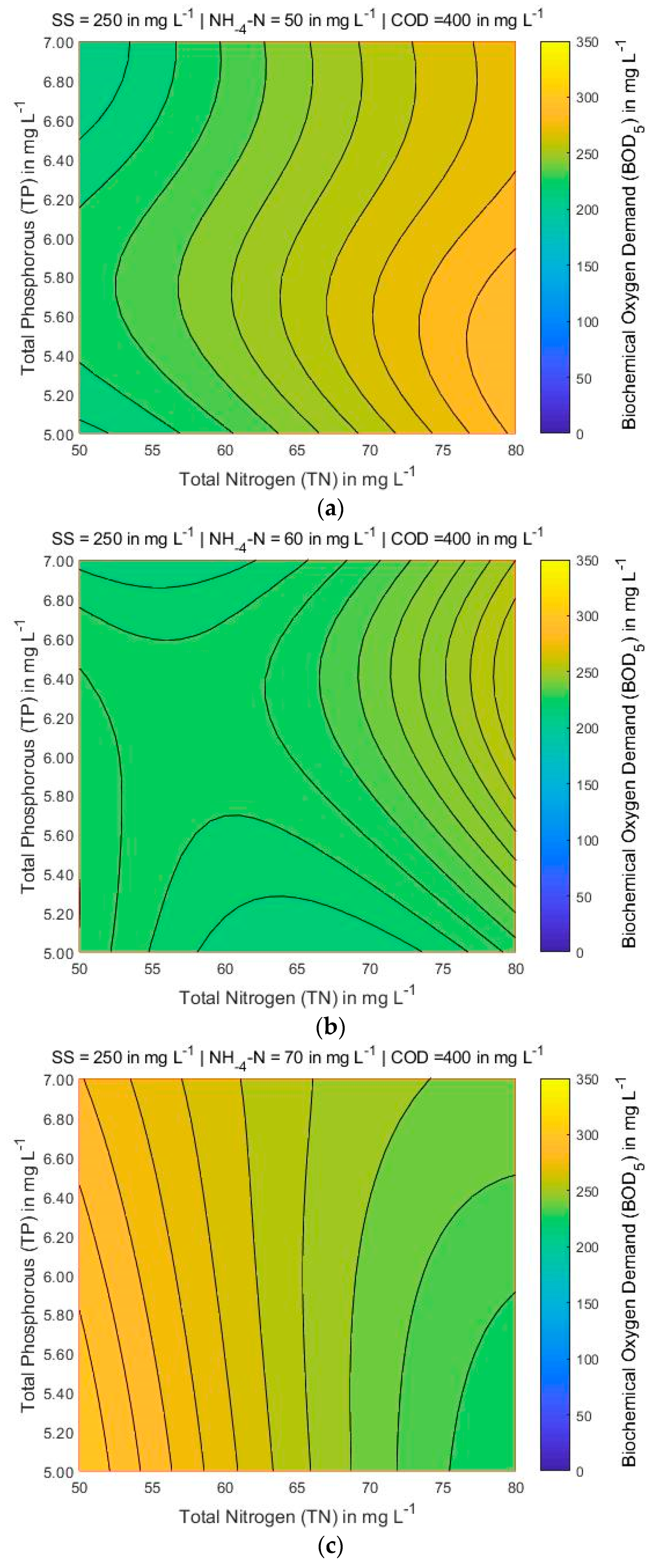
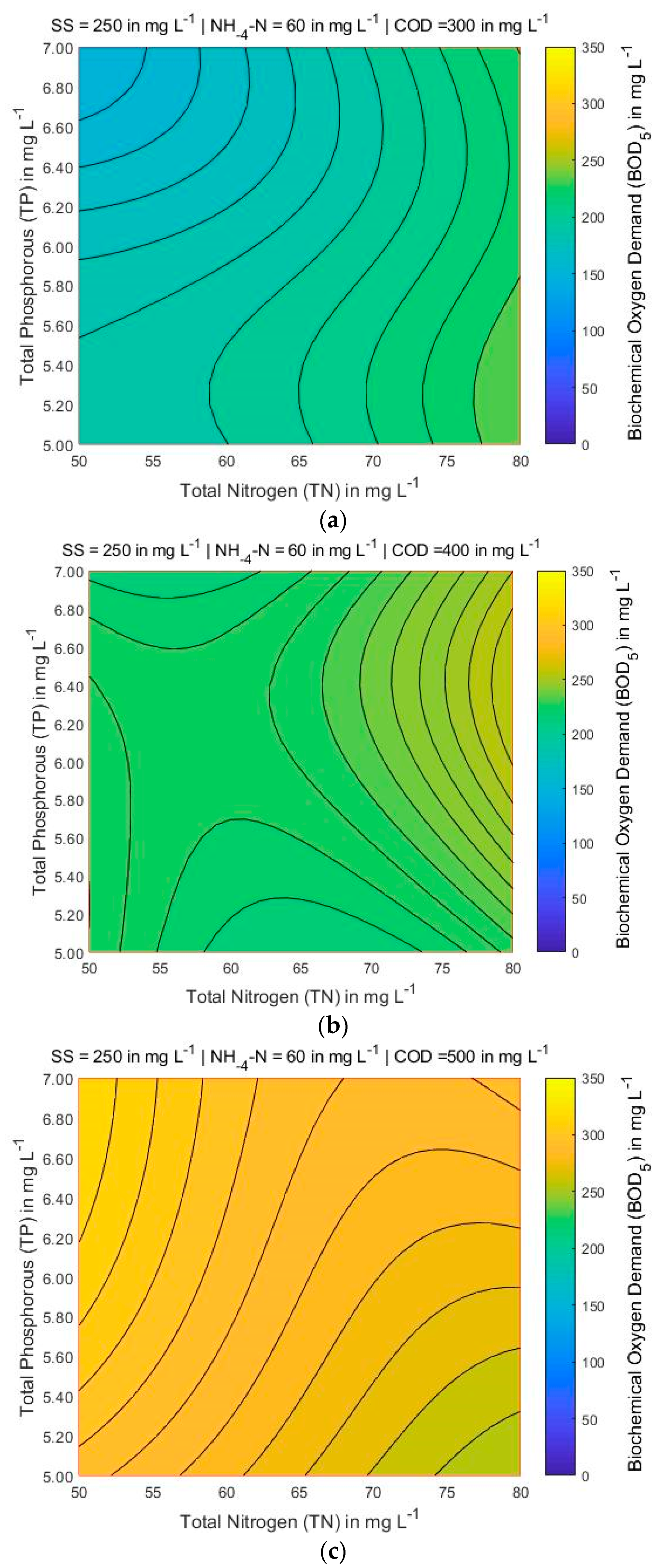
With the proposed optimal ANN-LM 5-8-1 model, a thorough analytical investigation was conducted of the parameters that affect the value of BOD₅. Based on the results of this analytical investigation they were derived a set of contour maps of the BOD₅ in relation of the input parameters (Figure 7, Figure 8, Figure 9, Figure 10, Figure 11 and Figure 12). Based on these figures, it is shown in a robust manner that the proposed ANN-LM 5-8-1 model ensures that the known and widely encountered phenomenon of overfitting is not taking place. This is implied by the fact that all the derived charts and the derived curves are exceptionally smooth and do not display sudden variations having as a result to exhibit the laws that govern the variation of BOD₅ concerning COD, SS, TN, NH₄-N and TP.

Figure 7 shows that for the lowest COD and TN values, the BOD also has the lowest value, searching all over the map area when NH4-N and TP are 60 and 8 mg L⁻¹, respectively, and SS varies between 200 and 300 mg L⁻¹. Figure 8 and Figure 9, the variations of COD and TN present smooth curvature, searching all over the map area. A more detailed look at Figure 8 (left corner) shows that the lowest contents of COD and TN, the BOD presents the highest value only in one part of the map. It is found that the COD and TN are sensitive to BOD parameter. Figure 10, Figure 11 and Figure 12 presents that for lowest contents of TP and TN, the BOD has moderate value when SS ranges from 250 and 300 mg L⁻¹, and NH₄-N and COD is 60 and 400 mg L⁻¹, respectively. A more detailed look at Figure 12, presents that the lowest concentrations of TP and TN, the BOD shows the highest value in the significant part of the map.

5. Limitations and Future Works

The proposed optimal ANN-LM 5-8-1 model, like any other mathematical simulant, has validity for values of the input parameters between the minimum and maximum values of the database that was used for the training of ANN models (Table 3). Additionally, the reliability of the proposed model is exceptionally high for ranges of the values of the parameters where according to the histograms that were presented in the previous section (Figure 3), there exists sufficient data. For the regions where the data are not considered enough, we must update the database with further data that cover these areas satisfactorily. Based on those mentioned above, the authors’ aims include updating the database and data from measurements from different sewage processing plants with the target of formulating one even more reliable model for estimating BOD₅ in wastewater.

6. Conclusions

The proposed ANN LM 5-8-1 approach can save costs and time for actual laboratory measurements. In other words, it is a practical need to illustrate a machine learning approach to conduct BOD estimation and receive accurate findings. The variation of COD and TN exhibit smooth curvature. COD and TN are found to be sensitive to the BOD parameter. The proposed optimal ANN model is valid for input parameter values between the minimum and maximum values of the database used for ANN model training. Furthermore, the proposed model’s reliability is exceptionally high for parameter value ranges where there is sufficient data. The developed and proposed ANN model proved to be a robust and valuable tool for scientists, researchers, engineers and practitioners in monitoring water systems and the design phase of wastewater treatment plants. Moreover, it is an illustrative example of ANN methodology for environmental and educational applications.

References

- Jouanneau, S.; Recoules, L.; Durand, M.J.; Boukabache, A.; Picot, V.; Primault, Y.; Lakel, A.; Sengelin, M.; Barillon, B.; Thouand, G. Methods for Assessing Biochemical Oxygen Demand (BOD): A Review. Water Res. 2014, 49, 62–82. [Google Scholar] [CrossRef] [PubMed]
- Riedel, K.; Kunze, G.; König, A. Microbial Sensors on a Respiratory Basis for Wastewater Monitoring. In History and Trends in Bioprocessing and Biotransformation; Dutta, N.N., Hammar, F., Haralampidis, K., Karanth, N.G., König, A., Krishna, S.H., Kunze, G., Nagy, E., Orlich, B., Osbourn, A.E., et al., Eds.; Advances in Biochemical Engineering/Biotechnology; Springer: Berlin/Heidelberg, Germany, 2002; Volume 75, pp. 81–118. ISBN 978-3-540-42371-3. [Google Scholar]
- Ngoc, L.T.B.; Tu, T.A.; Hien, L.T.T.; Linh, D.N.; Tri, N.; Duy, N.P.H.; Cuong, H.T.; Phuong, P.T.T. Simple Approach for the Rapid Estimation of BOD5 in Food Processing Wastewater. Environ. Sci. Pollut. Res. 2020, 27, 20554–20564. [Google Scholar] [CrossRef]
- Alexakis, D.; Kagalou, I.; Tsakiris, G. Assessment of Pressures and Impacts on Surface Water Bodies of the Mediterranean. Case Study: Pamvotis Lake, Greece. Environ. Earth Sci. 2013, 70, 687–698. [Google Scholar] [CrossRef]
- Alexakis, D.; Tsihrintzis, V.A.; Tsakiris, G.; Gikas, G.D. Suitability of Water Quality Indices for Application in Lakes in the Mediterranean. Water Resour. Manag. 2016, 30, 1621–1633. [Google Scholar] [CrossRef]
- Gamvroula, D.E.; Alexakis, D.E. Evaluating the Performance of Water Quality Indices: Application in Surface Water of Lake Union, Washington State-USA. Hydrology 2022, 9, 116. [Google Scholar] [CrossRef]
- Cheng, S.; Lin, Z.; Sun, Y.; Li, H.; Ren, X. Fast and Simultaneous Detection of Dissolved BOD and Nitrite in Wastewater by Using Bioelectrode with Bidirectional Extracellular Electron Transport. Water Res. 2022, 213, 118186. [Google Scholar] [CrossRef] [PubMed]
- Zeinolabedini, M.; Najafzadeh, M. Comparative Study of Different Wavelet-Based Neural Network Models to Predict Sewage Sludge Quantity in Wastewater Treatment Plant. Environ. Monit. Assess. 2019, 191, 163. [Google Scholar] [CrossRef]
- Najafzadeh, M.; Zeinolabedini, M. Derivation of Optimal Equations for Prediction of Sewage Sludge Quantity Using Wavelet Conjunction Models: An Environmental Assessment. Environ. Sci. Pollut. Res. 2018, 25, 22931–22943. [Google Scholar] [CrossRef]
- Najafzadeh, M.; Zeinolabedini, M. Prognostication of Waste Water Treatment Plant Performance Using Efficient Soft Computing Models: An Environmental Evaluation. Measurement 2019, 138, 690–701. [Google Scholar] [CrossRef]
- Gunjal, S.; Khobragade, M.; Chaware, C. Prediction of BOD from Wastewater Characteristics and Their Interactions Using Regression Neural Network: A Case Study of Naidu Wastewater Treatment Plant, Pune, India. In Recent Trends in Construction Technology and Management; Ranadive, M.S., Das, B.B., Mehta, Y.A., Gupta, R., Eds.; Lecture Notes in Civil Engineering; Springer Nature: Singapore, 2023; Volume 260, pp. 571–577. ISBN 978-981-19214-4-5. [Google Scholar]
- Hu, Y.; Du, W.; Yang, C.; Wang, Y.; Huang, T.; Xu, X.; Li, W. Source Identification and Prediction of Nitrogen and Phosphorus Pollution of Lake Taihu by an Ensemble Machine Learning Technique. Front. Environ. Sci. Eng. 2023, 17, 55. [Google Scholar] [CrossRef]
- Ismail, S.; Ahmed, M.F. Hydrogeochemical Characterization of the Groundwater of Lahore Region Using Supervised Machine Learning Technique. Environ. Monit. Assess. 2023, 195, 5. [Google Scholar] [CrossRef] [PubMed]
- Zhou, P.; Li, Z.; El-Dakhakhni, W.; Smyth, S.A. Prediction of Bisphenol A Contamination in Canadian Municipal Wastewater. J. Water Process Eng. 2022, 50, 103304. [Google Scholar] [CrossRef]
- Zhong, H.; Yuan, Y.; Luo, L.; Ye, J.; Chen, M.; Zhong, C. Water Quality Prediction of MBR Based on Machine Learning: A Novel Dataset Contribution Analysis Method. J. Water Process Eng. 2022, 50, 103296. [Google Scholar] [CrossRef]
- Jordan, M.I.; Mitchell, T.M. Machine Learning: Trends, Perspectives, and Prospects. Science 2015, 349, 255–260. [Google Scholar] [CrossRef] [PubMed]
- Huang, R.; Ma, C.; Ma, J.; Huangfu, X.; He, Q. Machine Learning in Natural and Engineered Water Systems. Water Res. 2021, 205, 117666. [Google Scholar] [CrossRef]
- ISO 5815-1:2003; Water Quality-Determination of Biochemical Oxygen Demand after N Days (BODn)-Part 1: Dilution and Seeding Method with Allylthiourea Addition. International Organization for Standardization: Geneva, Switzerland, 2003.
- McDonagh, C.; Kolle, C.; McEvoy, A.K.; Dowling, D.L.; Cafolla, A.A.; Cullen, S.J.; MacCraith, B.D. Phase Fluorometric Dissolved Oxygen Sensor. Sens. Actuators B Chem. 2001, 74, 124–130. [Google Scholar] [CrossRef]
- McEvoy, A.K.; McDonagh, C.M.; MacCraith, B.D. Dissolved Oxygen Sensor Based on Fluorescence Quenching of Oxygen-Sensitive Ruthenium Complexes Immobilized in Sol–Gel-Derived Porous Silica Coatings. Analyst 1996, 121, 785–788. [Google Scholar] [CrossRef]
- Xiong, X.; Xiao, D.; Choi, M.F. Dissolved Oxygen Sensor Based on Fluorescence Quenching of Oxygen-Sensitive Ruthenium Complex Immobilized on Silica–Ni–P Composite Coating. Sens. Actuators B Chem. 2006, 117, 172–176. [Google Scholar] [CrossRef]
- Xu, W.; McDonough, R.C.; Langsdorf, B.; Demas, J.N.; DeGraff, B.A. Oxygen Sensors Based on Luminescence Quenching: Interactions of Metal Complexes with the Polymer Supports. Anal. Chem. 1994, 66, 4133–4141. [Google Scholar] [CrossRef]
- Sakaguchi, T.; Kitagawa, K.; Ando, T.; Murakami, Y.; Morita, Y.; Yamamura, A.; Yokoyama, K.; Tamiya, E. A Rapid BOD Sensing System Using Luminescent Recombinants of Escherichia Coli. Biosens. Bioelectron. 2003, 19, 115–121. [Google Scholar] [CrossRef]
- Sakaguchi, T.; Morioka, Y.; Yamasaki, M.; Iwanaga, J.; Beppu, K.; Maeda, H.; Morita, Y.; Tamiya, E. Rapid and Onsite BOD Sensing System Using Luminous Bacterial Cells-Immobilized Chip. Biosens. Bioelectron. 2007, 22, 1345–1350. [Google Scholar] [CrossRef] [PubMed]
- Kim, B.H.; Chang, I.S.; Cheol Gil, G.; Park, H.S.; Kim, H.J. Novel BOD (Biological Oxygen Demand) Sensor Using Mediator-Less Microbial Fuel Cell. Biotechnol. Lett. 2003, 25, 541–545. [Google Scholar] [CrossRef] [PubMed]
- Karube, I.; Matsunaga, T.; Mitsuda, S.; Suzuki, S. Microbial Electrode BOD Sensors. Biotechnol. Bioeng. 1977, 19, 1535–1547. [Google Scholar] [CrossRef] [PubMed]
- Liu, C.; Zhao, H.; Zhong, L.; Liu, C.; Jia, J.; Xu, X.; Liu, L.; Dong, S. A Biofilm Reactor-Based Approach for Rapid on-Line Determination of Biodegradable Organic Pollutants. Biosens. Bioelectron. 2012, 34, 77–82. [Google Scholar] [CrossRef]
- Zare Abyaneh, H. Evaluation of Multivariate Linear Regression and Artificial Neural Networks in Prediction of Water Quality Parameters. J. Environ. Health Sci. Eng. 2014, 12, 40. [Google Scholar] [CrossRef] [Green Version]
- Singh, K.P.; Basant, A.; Malik, A.; Jain, G. Artificial Neural Network Modeling of the River Water Quality—A Case Study. Ecol. Model. 2009, 220, 888–895. [Google Scholar] [CrossRef]
- Ahmed, A.A.M.; Shah, S.M.A. Application of Adaptive Neuro-Fuzzy Inference System (ANFIS) to Estimate the Biochemical Oxygen Demand (BOD) of Surma River. J. King Saud Univ. Eng. Sci. 2017, 29, 237–243. [Google Scholar] [CrossRef] [Green Version]
- Basant, N.; Gupta, S.; Malik, A.; Singh, K.P. Linear and Nonlinear Modeling for Simultaneous Prediction of Dissolved Oxygen and Biochemical Oxygen Demand of the Surface Water—A Case Study. Chemom. Intell. Lab. Syst. 2010, 104, 172–180. [Google Scholar] [CrossRef]
- Asami, H.; Golabi, M.; Albaji, M. Simulation of the Biochemical and Chemical Oxygen Demand and Total Suspended Solids in Wastewater Treatment Plants: Data-Mining Approach. J. Clean. Prod. 2021, 296, 126533. [Google Scholar] [CrossRef]
- McCulloch, W.S.; Pitts, W. A Logical Calculus of the Ideas Immanent in Nervous Activity. Bull. Math. Biophys. 1943, 5, 115–133. [Google Scholar] [CrossRef]
- Gavriilaki, E.; Asteris, P.G.; Touloumenidou, T.; Koravou, E.-E.; Koutra, M.; Papayanni, P.G.; Karali, V.; Papalexandri, A.; Varelas, C.; Chatzopoulou, F.; et al. Genetic Justification of Severe COVID-19 Using a Rigorous Algorithm. Clin. Immunol. 2021, 226, 108726. [Google Scholar] [CrossRef] [PubMed]
- Asteris, P.G.; Gavriilaki, E.; Touloumenidou, T.; Koravou, E.; Koutra, M.; Papayanni, P.G.; Pouleres, A.; Karali, V.; Lemonis, M.E.; Mamou, A.; et al. Genetic Prediction of ICU Hospitalization and Mortality in COVID-19 Patients Using Artificial Neural Networks. J. Cell. Mol. Med. 2022, 26, 1445–1455. [Google Scholar] [CrossRef] [PubMed]
- Upadhyay, A.K.; Shukla, S. Correlation Study to Identify the Factors Affecting COVID-19 Case Fatality Rates in India. Diabetes Metab. Syndr. Clin. Res. Rev. 2021, 15, 993–999. [Google Scholar] [CrossRef] [PubMed]
- Niazkar, H.R.; Niazkar, M. Application of Artificial Neural Networks to Predict the COVID-19 Outbreak. Glob. Health Res. Policy 2020, 5, 50. [Google Scholar] [CrossRef] [PubMed]
- Mahanty, C.; Kumar, R.; Asteris, P.G.; Gandomi, A.H. COVID-19 Patient Detection Based on Fusion of Transfer Learning and Fuzzy Ensemble Models Using CXR Images. Appl. Sci. 2021, 11, 11423. [Google Scholar] [CrossRef]
- Rahimi, I.; Gandomi, A.H.; Asteris, P.G.; Chen, F. Analysis and Prediction of COVID-19 Using SIR, SEIQR, and Machine Learning Models: Australia, Italy, and UK Cases. Information 2021, 12, 109. [Google Scholar] [CrossRef]
- Asteris, P.G.; Douvika, M.G.; Karamani, C.A.; Skentou, A.D.; Chlichlia, K.; Cavaleri, L.; Daras, T.; Armaghani, D.J.; Zaoutis, T.E. A Novel Heuristic Algorithm for the Modeling and RiskAssessment of the COVID-19 Pandemic Phenomenon. Comput. Model. Eng. Sci. 2020, 125, 815–828. [Google Scholar] [CrossRef]
- APHA; AWWA; WPCF. Standard Methods for the Examination of Water and Wastewater, 20th ed.; American Public Health Association: Washington, DC, USA, 1999. [Google Scholar]
- Jong, Y.-H.; Lee, C.-I. Influence of Geological Conditions on the Powder Factor for Tunnel Blasting. Int. J. Rock Mech. Min. Sci. 2004, 41, 533–538. [Google Scholar] [CrossRef]
- Bardhan, A.; Biswas, R.; Kardani, N.; Iqbal, M.; Samui, P.; Singh, M.P.; Asteris, P.G. A Novel Integrated Approach of Augmented Grey Wolf Optimizer and ANN for Estimating Axial Load Carrying-Capacity of Concrete-Filled Steel Tube Columns. Constr. Build. Mater. 2022, 337, 127454. [Google Scholar] [CrossRef]
- Mahmood, W.; Mohammed, A.S.; Asteris, P.G.; Kurda, R.; Armaghani, D.J. Modeling Flexural and Compressive Strengths Behaviour of Cement-Grouted Sands Modified with Water Reducer Polymer. Appl. Sci. 2022, 12, 1016. [Google Scholar] [CrossRef]
- Mahmood, W.; Mohammed, A.S.; Sihag, P.; Asteris, P.G.; Ahmed, H. Interpreting the Experimental Results of Compressive Strength of Hand-Mixed Cement-Grouted Sands Using Various Mathematical Approaches. Arch. Civ. Mech. Eng. 2022, 22, 19. [Google Scholar] [CrossRef]
- Emad, W.; Salih, A.; Kurda, R.; Asteris, P.G.; Hassan, A. Nonlinear Models to Predict Stress versus Strain of Early Age Strength of Flowable Ordinary Portland Cement. Eur. J. Environ. Civ. Eng. 2022, 26, 8433–8457. [Google Scholar] [CrossRef]
- Asteris, P.G.; Apostolopoulou, M.; Armaghani, D.J.; Cavaleri, L.; Chountalas, A.T.; Guney, D.; Hajihassani, M.; Hasanipanah, M.; Khandelwal, M.; Karamani, C.; et al. On the Metaheuristic Models for the Prediction of Cement-Metakaolin Mortars Compressive Strength. Metaheu Comp. Appl. 2020, 1, 63–69. [Google Scholar] [CrossRef]
- Asteris, P.G.; Argyropoulos, I.; Cavaleri, L.; Rodrigues, H.; Varum, H.; Thomas, J.; Lourenço, P.B. Masonry Compressive Strength Prediction Using Artificial Neural Networks. In Transdisciplinary Multispectral Modeling and Cooperation for the Preservation of Cultural Heritage; Moropoulou, A., Korres, M., Georgopoulos, A., Spyrakos, C., Mouzakis, C., Eds.; Communications in Computer and Information Science; Springer International Publishing: Cham, Switzerland, 2019; Volume 962, pp. 200–224. ISBN 978-3-030-12959-0. [Google Scholar]
- Armaghani, D.J.; Asteris, P.G.; Fatemi, S.A.; Hasanipanah, M.; Tarinejad, R.; Rashid, A.S.A.; Huynh, V.V. On the Use of Neuro-Swarm System to Forecast the Pile Settlement. Appl. Sci. 2020, 10, 1904. [Google Scholar] [CrossRef] [Green Version]
- Lu, S.; Koopialipoor, M.; Asteris, P.G.; Bahri, M.; Armaghani, D.J. A Novel Feature Selection Approach Based on Tree Models for Evaluating the Punching Shear Capacity of Steel Fiber-Reinforced Concrete Flat Slabs. Materials 2020, 13, 3902. [Google Scholar] [CrossRef]
- Le, T.-T. Practical Machine Learning-Based Prediction Model for Axial Capacity of Square CFST Columns. Mech. Adv. Mater. Struct. 2022, 29, 1782–1797. [Google Scholar] [CrossRef]
- Le, T.-T.; Asteris, P.G.; Lemonis, M.E. Prediction of Axial Load Capacity of Rectangular Concrete-Filled Steel Tube Columns Using Machine Learning Techniques. Eng. Comput. 2022, 38, 3283–3316. [Google Scholar] [CrossRef]
- Le, T.-T.; Le, M.V. Development of User-Friendly Kernel-Based Gaussian Process Regression Model for Prediction of Load-Bearing Capacity of Square Concrete-Filled Steel Tubular Members. Mater. Struct. 2021, 54, 59. [Google Scholar] [CrossRef]
- Armaghani, D.J.; Asteris, P.G. A Comparative Study of ANN and ANFIS Models for the Prediction of Cement-Based Mortar Materials Compressive Strength. Neural Comput. Appl. 2021, 33, 4501–4532. [Google Scholar] [CrossRef]
- Asteris, P.G.; Mokos, V.G. Concrete Compressive Strength Using Artificial Neural Networks. Neural Comput. Appl. 2020, 32, 11807–11826. [Google Scholar] [CrossRef]
- Asteris, P.G.; Nguyen, T.-A. Prediction of Shear Strength of Corrosion Reinforced Concrete Beams Using Artificial Neural Network. J. Sci. Transp. Tech. 2022, 2, 1–12. [Google Scholar]
- Li, N.; Asteris, P.G.; Tran, T.-T.; Pradhan, B.; Nguyen, H. Modelling the Deflection of Reinforced Concrete Beams Using the Improved Artificial Neural Network by Imperialist Competitive Optimization. Steel Compos. Struct. 2022, 42, 733–745. [Google Scholar] [CrossRef]
- Lemonis, M.E.; Daramara, A.G.; Georgiadou, A.G.; Siorikis, V.G.; Tsavdaridis, K.D.; Asteris, P.G. Ultimate Axial Load of Rectangular Concrete-Filled Steel Tubes Using Multiple ANN Activation Functions. Steel Compos. Struct. 2022, 42, 459–475. [Google Scholar] [CrossRef]
- Asteris, P.G.; Rizal, F.I.M.; Koopialipoor, M.; Roussis, P.C.; Ferentinou, M.; Armaghani, D.J.; Gordan, B. Slope Stability Classification under Seismic Conditions Using Several Tree-Based Intelligent Techniques. Appl. Sci. 2022, 12, 1753. [Google Scholar] [CrossRef]
- Asteris, P.G.; Lourenço, P.B.; Hajihassani, M.; Adami, C.-E.N.; Lemonis, M.E.; Skentou, A.D.; Marques, R.; Nguyen, H.; Rodrigues, H.; Varum, H. Soft Computing-Based Models for the Prediction of Masonry Compressive Strength. Eng. Struct. 2021, 248, 113276. [Google Scholar] [CrossRef]
- Asteris, P.G.; Skentou, A.D.; Bardhan, A.; Samui, P.; Lourenço, P.B. Soft Computing Techniques for the Prediction of Concrete Compressive Strength Using Non-Destructive Tests. Constr. Build. Mater. 2021, 303, 124450. [Google Scholar] [CrossRef]
- Asteris, P.G.; Koopialipoor, M.; Armaghani, D.J.; Kotsonis, E.A.; Lourenço, P.B. Prediction of Cement-Based Mortars Compressive Strength Using Machine Learning Techniques. Neural Comput. Appl. 2021, 33, 13089–13121. [Google Scholar] [CrossRef]
Figure 1.
Architecture of an ANN model composed of one hidden layer.
Figure 2.
Pearson correlation coefficients between the examined variables.
Figure 3.
Scatter plots and histograms of the studied input and output parameters: (a,b) COD; (c,d) SS; (e,f) TN; (g,h) NH4-N; (i,j) TP; and (k,l) BOD5.
Figure 4.
Sensitivity analysis of the Biochemical Oxygen Demand (BOD5) on input parameters based on the experimental database.
Figure 5.
Architecture of the optimum ANN LM 5-8-1 model.
Figure 6.
Experimental vs. predicted values of the five-day biochemical oxygen demand (BOD5) in wastewater for training and testing datasets, using the developed ANN LM 5-8-1 model.
Figure 7.
BOD5 contour maps for three different values of SS (in mg L−1) while NH4-N = 60 mg L−1 and TP = 8 mg L−1 are constant: (a) SS = 200; (b) SS = 250; and (c) SS = 300.
Figure 8.
BOD5 contour maps for three different values of NH4-N (in mg L−1) while SS = 250 mg L−1 and TP = 8 mg L−1 are constant: (a) NH4-N = 50; (b) NH4-N = 60; and (c) NH4-N = 70.
Figure 9.
BOD5 contour maps for three different values of TP (in mg L−1) while SS = 250 mg L−1 and NH4-N = 60 mg L−1 are constant: (a) TP = 6; (b) TP = 8; and (c) TP = 10.
Figure 10.
BOD5 contour maps for three different values of SS (in mg L−1) while NH4N = 60 mg L−1 and COD = 400 mg L−1 are constant: (a) SS = 200; (b) SS = 250; and (c) SS = 300.
Figure 11.
BOD5 contour maps for three different values of NH4-N (in mg L−1) while SS = 250 mg L−1 and COD = 400 mg L−1 are constant: (a) NH4-N = 50; (b) NH4-N = 60; and (c) NH4-N = 70.
Figure 12.
BOD5 contour maps for three different values of COD (in mg L−1) while SS = 250 mg L−1 and NH4-N = 60 mg L−1 are constant: (a) COD = 300; (b) COD = 400; and (c) COD = 500.