

Risk Assessment of Dike Based on Risk Chain Model and Fuzzy Influence Diagram

College of Mechanics and Materials, Hohai University, Nanjing 211100, China
*
Author to whom correspondence should be addressed.
Water 2023, 15(1), 108; https://doi.org/10.3390/w15010108
Submission received: 22 November 2022
/
Revised: 23 December 2022
/
Accepted: 26 December 2022
/
Published: 28 December 2022
(This article belongs to the Special Issue Safety Evaluation of Dam and Geotechnical Engineering)
Abstract
:For the risk assessment of flood defense, a comprehensive understanding of risk factors affecting dike failure is essential. Traditional risk assessment methods are mostly based on experts’ experience and focus on just one type of failure mode of flood defensive structures. The risk resources, including the analytical factors and non-analytical factors, were summarized firstly according to the general experience of dikes. The uncertainty of the resources that affect dike safety can be quantified by membership degree. Hence, a fuzzy influence diagram based on fuzzy mathematics was proposed to assess the safety of the dikes. We evaluated the multi-failure modes at the same time by a fuzzy influence diagram. Taking a dike as an example, the expected value of the dike failure was 6.25%. Furthermore, the chance of damage to this dike was “very unlikely” according to the descriptive term of the Intergovernmental Panel on Climate Change (IPCC). The evaluation result was obtained as a probabilistic value, which enabled an intuitive perception of the safety of the dikes. Therefore, we provided some reasonable suggestions for project management and regular maintenance. Since the proposed method can account for uncertainties, it is well suited for the risk assessment of dikes with obvious uncertainties.
1. Background
Dikes play an important role in the flood defense system of China. It was reported there were around 320,000 km of dikes to protect more than 640 million people and numerous cities [1]. Therefore, how to manage dikes using a reasonable method is an important task for reducing flood disaster. Because of some historical reasons, dikes in China were constructed in ancient times, and many dikes were made with local materials. As a result, the design standard and strength of the dikes located in remote areas of China are relatively low. Therefore, conducting the risk assessment of the dikes and discovering the hidden dangers in time are significant to protect the life and property of every citizen in the dike-protected areas.
In recent years, the traditional management of the dikes gradually changed to risk management. Developed countries, such as the UK, the Netherlands, and Japan, have taken the lead in introducing risk management methods into the risk assessment of dikes. For example, Mouri et al. [2] adopted the probability method to conduct the risk assessment of flooding considering natural and societal factors. Marijnissen et al. [3] used an extensive probabilistic method to re-evaluate the multifunctional dikes in the Netherlands considering the society and economy. Balistrocchi et al. [4] discussed the advantages of the two methods, i.e., numerical simulations and fragility curves, to study the failure probability analysis of levees. He proposed a model to calculate the failure probability of a mammal bioerosion levee considering the peak flow discharge and flood duration. Agbaje et al. [5] studied the influence of the effective friction angle on slope stability based on the Grag deposits in the East of England, UK. It pointed out that the total factor of safety was usually higher, leading to overestimation of the stability of a slope.
There are three main failure modes in China: overtopping, scouring, and seepage [6]. If the crest of the dike is below the run-up level, the waves will cause a flow of water over the top of the dike, across the crest, and onto the landside slope. This phenomenon is called overtopping. The pore pressure affects the stability of the levee body and/or foundation through infiltration and affects the back erosion piping or slope stability. This phenomenon is called seepage failure. Scouring failure is the damage caused by the water flow and waves, which usually leads to dangerous situations such as the inner slope collapse of the dike. Overtopping failure is considered a kind of hydrology failure, and the scouring and seepage failures are considered structural failures. However, most of the risk analyses focused on one of the above three failure mechanisms by only considering the analytical factors. For example, the risk analysis of overtopping was used to measure the overtopping failure [7,8,9,10,11,12,13,14]; the scouring analysis and slope stability analysis were conducted only for the dike body [15,16,17,18,19]; and most seepage analyses were also performed separately [20,21,22]. There were a few pieces of literature that assessed dike damage by considering failure modes with both analytical and non-analytical factors [23].
In another way, the traditional models, including the analytic hierarchy process, event tree method, and fault tree method, are mainly used to perform the system risk assessment. Song et al. [24] studied the risk assessment of tunnel construction based on the fuzzy analytic hierarchy process. Wang et al. [25] used a fuzzy analytic hierarchy process to identify the safety mode of the section of Jingnan dike that is located in Jingzhou City, China. Gu et al. [26] proposed an experts’ weighting model for the safety evaluation of a dike using fuzzy mathematics and the dynamic clustering method. The analytic hierarchy process mostly relies on the subjective experts’ experience and evaluates only using the appearance, which often leads to deviation in the evaluation results [27]. Fault tree and event tree analysis methods are widely used; however, the accurate probability value of basic events needs to be known in the calculation process [28].
The influence diagram method is a risk assessment method proposed by Howard [29]. The influence diagram is composed of two parts, the risk node and the risk relationship. It can represent the directed graph of the mutual influence between the risk elements and can provide relatively accurate calculation results for risk assessment. Moreover, it is also suitable for the risk assessment of system engineering. A fuzzy influence diagram is a combination of the fuzzy set, fuzzy transformation method, and influence diagram method to carry out probabilistic inferences on uncertain events. During the inference process, the occurrence probability of an event and the occurrence probability of other dependent events can be fully evaluated. Due to the advantages of intuition and easy understanding, the application scope of the fuzzy influence diagram is gradually expanding. Based on the 3D Hall structure model of system engineering, the risk identification method of overseas nuclear power projects was optimized by considering the idea of risk chain and risk map [30]. Xu et al. [31] used the fuzzy influence diagram to evaluate the construction safety risk of power transmission and transformation engineering construction projects. Quan et al. [32,33] conducted a qualitative risk analysis on the general contracting of overseas EPC power engineering projects using the fuzzy influence diagram method. Later, Zhang et al. [34] introduced the fuzzy influence diagram method into the risk assessment process of information security and introduced fuzzy theory to describe risk factors that are difficult to quantify and to obtain good results. Lin et al. [35] applied the fuzzy influence diagram method to the safety management of underground pipelines and focused on the analysis of the risks caused by external force damage. To the best knowledge of the authors, this is the first time using the risk chain model and fuzzy influence diagram method to evaluate dike safety. Theoretically, the fuzzy influence diagram method is based on fuzzy mathematics. The introduction of state fuzzy sets, frequency fuzzy sets, and membership degrees can fully consider the uncertainty of the risk factors and at the same time reduce the subjectivity of experts’ judgment. It is suitable to perform the risk assessment for the dikes with uncertainty and complexity.
This present study aimed to (1) summarize the risk resources that affect dike safety based on the general experience of the dikes; (2) analyze the relationships between the risk resources and risk events; (3) construct a fuzzy influence diagram based on (1) and (2); and (4) take a fictitious dike as an example to illustrate the proposed method and apply the description term of IPCC to the result.
2. The Risk Chain Model and the Fuzzy Influence Diagram
2.1. The Risk Chain Model
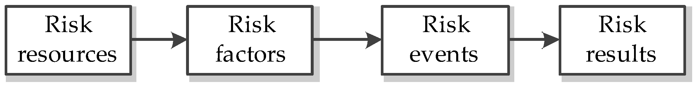
A fuzzy influence diagram is a graph composed of multiple risk chains, and each risk chain can be regarded as an independent logical relationship. A risk chain is established by adding nodes such as risk sources, risk factors, and risk events in layers. Within an assessment system, different risk chains should ultimately point to the same risk consequence. The risk chain structure is shown in Figure 1.
2.2. Fuzzy Set and Membership Function
2.2.1. The Definition of Fuzzy Set and Membership
The introduction of fuzzy sets in this paper is limited to the case where the universe of discourse is a finite set, denoted by . Mapping on the domain , , then , the fuzzy set was determined. is the membership function of , and is the membership degree of a to the fuzzy set , denoted as:
The algorithm of the fuzzy influence graph is based on fuzzy set operation and uses a directed graph to describe the state, frequency, and relationship between nodes, and then it carries out a risk assessment for the system.
2.2.2. The Operations on Fuzzy Sets
We briefly describe the three operation notations of the fuzzy set used in this paper. The symbol “×” is a Cartesian product. If and are fuzzy sets of two universes and , respectively, then the fuzzy relation from to is:
A fuzzy relation is a special kind of fuzzy set, and the result is a fuzzy matrix.
The symbol “∘” is called fuzzy synthesis, that is, dot product. If is a fuzzy relation from to , similarly, if is a fuzzy relation from to , then the fuzzy composition of and is:
The result of fuzzy synthesis is still a fuzzy matrix, representing the fuzzy relationship from to .
The symbol “” is called the “union” of fuzzy sets and has the following operations:
It should be pointed out here that “Cartesian product” and “dot product” should operate on fuzzy sets of different universes, and “union” should operate on fuzzy sets in the same universe.
2.3. The Process of the Fuzzy Influence Diagram
The fuzzy influence diagram introduces the state fuzzy set and the frequency fuzzy set in the numerical layer to describe the data structure of the node and uses the fuzzy relationship to describe the relationship between the node variables in the function layer. The calculation process of the fuzzy influence diagram is explained below [36].
2.3.1. The Calculation of Independent Node Frequency Matrix
If has no immediate predecessor, it is called an independent node, and it is assumed that the possible state vector of the independent node is:
where is the state fuzzy set defined by the risk assessor according to the actual situation. The frequency vector of an independent node is:
where is the state fuzzy set defined by the risk assessor according to the actual situation. The frequency vector of an independent node is:
2.3.2. The Calculation of the Frequency Matrix of Dependent Nodes
If is made up of m random nodes as its immediate predecessors, then is called a dependent node.
Define as the fuzzy relationship from node to dependent node :
where , . The fuzzy relationship from node to node is:
Then, the joint of the fuzzy relationship of all immediate predecessors of the dependent node is:
The frequency matrix of the dependent node can be obtained by the dot product relationship:
2.3.3. Result Analysis
The membership degree of the random result is selected from the frequency matrix of the risk consequence node by Equation (13), and the probability value of the result is calculated by Equation (14):
3. The Evaluation Process of the Fuzzy Influence Diagram
3.1. The Construction of the Frequency Fuzzy Set
For the convenience of calculation, combined with the experts’ experience on the dike, the frequency vector of the risk node of the dike was uniformly simplified to , as shown in Table 2. The frequency was processed as follows, and 0 to 1 were decomposed into (0.0, 0.1, 0.2, 0.3, 0.4, 0.5, 0.6, 0.7, 0.8, 0.9, 1.0), indicating the occurrence frequency of risk nodes. From the definition of fuzzy sets and membership degrees, the three fuzzy sets and their membership degrees of the frequency vector f of the dike risk node can be expressed as follows:
where the number above the symbol “—” is the frequency of node occurrence, and the number below represents the membership degree of the frequency. The number 0.7/0.5 means that the risk node is in the High Set, and the membership degree is 0.5 when the frequency of occurrence is 0.7. The number 0.7/0.2 means that the risk node is in the Medium Set, and the membership degree is 0.2 when the frequency is 0.7.
3.2. The Construction of the State Fuzzy Set
The state vector of the risk node in the fuzzy influence diagram is uniformly simplified as . The language description of the fuzzy set in the state vector has the same meaning as the description of the relationship between the nodes in Table 3. The state fuzzify sets and their membership functions are expressed as follows:
It is more appropriate to describe the states of some parts of nodes in the fuzzy influence diagram with certainty. Hence, it is necessary to artificially fuzzify them. In this paper, the states of all risk source nodes were artificially fuzzified. The membership functions are as follows:
3.3. Risk Assessment of One Dike Case
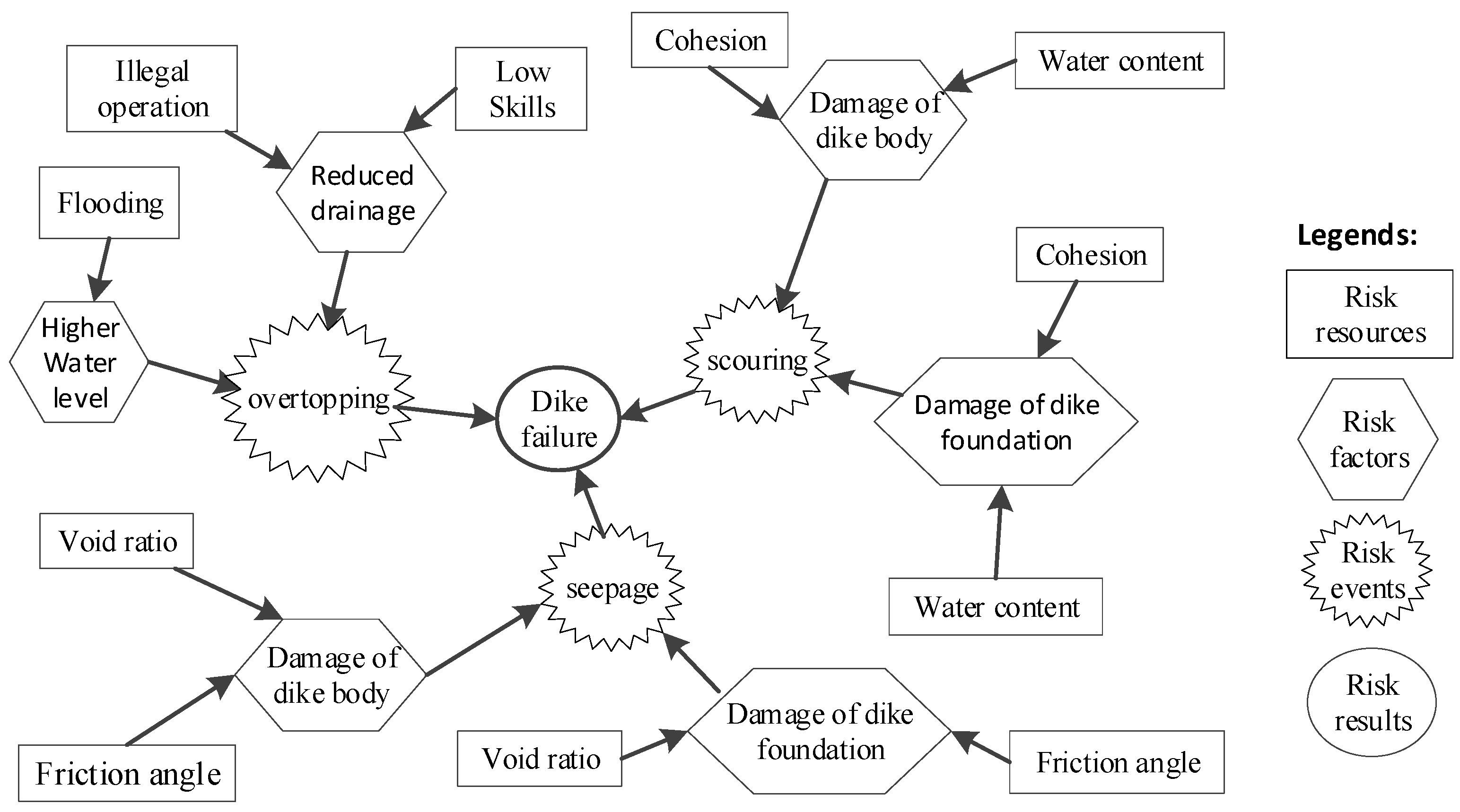
This paper sorted out the analytical factors and non-analytical factors that lead to dike failure and selected some factors that have an impact on the safety status of the dike as the risk source for analysis. The emergence of risk sources causes the occurrence of risk factors, which in turn leads to the occurrence of three common failure modes of dikes. The three failure modes comprehensively lead to dike failure (risk consequences). The constructed fuzzy influence diagram of dike failure is shown in Figure 2. According to the frequency fuzzy set, state fuzzy set, and fuzzy relationship constructed above, the calculation process of the risk chain “illegal operation-reduced drainage—overtopping—dike failure” was taken as an example, and the remaining evaluation process is similar to it.
Step 1, The frequency matrix of illegal operation risk source nodes is calculated by Equations (5)–(7):
In the same way, the frequency matrix of low-risk source nodes of security skills can be obtained.
Step 2, The joint frequency matrix of all immediate predecessor nodes of the node with reduced drainage capacity is calculated by Equation (8):
Step 3, The fuzzy relationship matrix from the node of illegal operation risk source to the node of drainage capacity reduction risk factor is calculated by Equation (10):
In the same way, the fuzzy relation matrix of the lower drainage capacity node caused by the low skills node can be obtained.
Step 4, The joint matrix of the fuzzy relationship of all immediately preceding nodes of the node that leads to the reduction of drainage capacity is calculated by Equation (11):
Similarly, the joint matrix of other fuzzy relations can be obtained.
Step 5, The frequency matrix of the nodes with reduced drained capacity is calculated by Equation (12):
In the same way, the frequency matrix of the node of rising water level in front of the dikes can be obtained. Thus far, the frequency matrix, the frequency joint matrix, the fuzzy relationship matrix between the nodes, and the fuzzy relationship joint matrix of any node can be obtained by analogy with the calculation process above.
Corresponding to the fuzzy relationship between the nodes in Table 3, the fuzzy influence diagram is completely calculated by analogy to the above calculation process. Only the calculation results of the key nodes in the subsequent calculation process of the fuzzy influence diagram are given here.
The relationship matrix from the drainage capacity reduction node to the overtopping risk event node is as follows:
The union of the fuzzy relationship matrices of all the immediate nodes of the overtopping risk event node is:
The frequency matrix of overtopping risk event nodes can be obtained as:
The joint frequency matrix of the three risk event nodes of overtopping, scouring, and seepage is:
The fuzzy relationship matrix of the overtopping failure mode to the dike failure node is:
The frequency matrix of risk consequence of dike failure nodes is:
By Equation (13), the row with the largest product value of the product of the frequency is selected, and the sum of the membership degrees of the row is calculated. In this example, it is the row corresponding to the frequency equal to 1.
The change probability of the dike failure node calculated by Equation (14) is:
The expected value of the increased risk can be calculated:
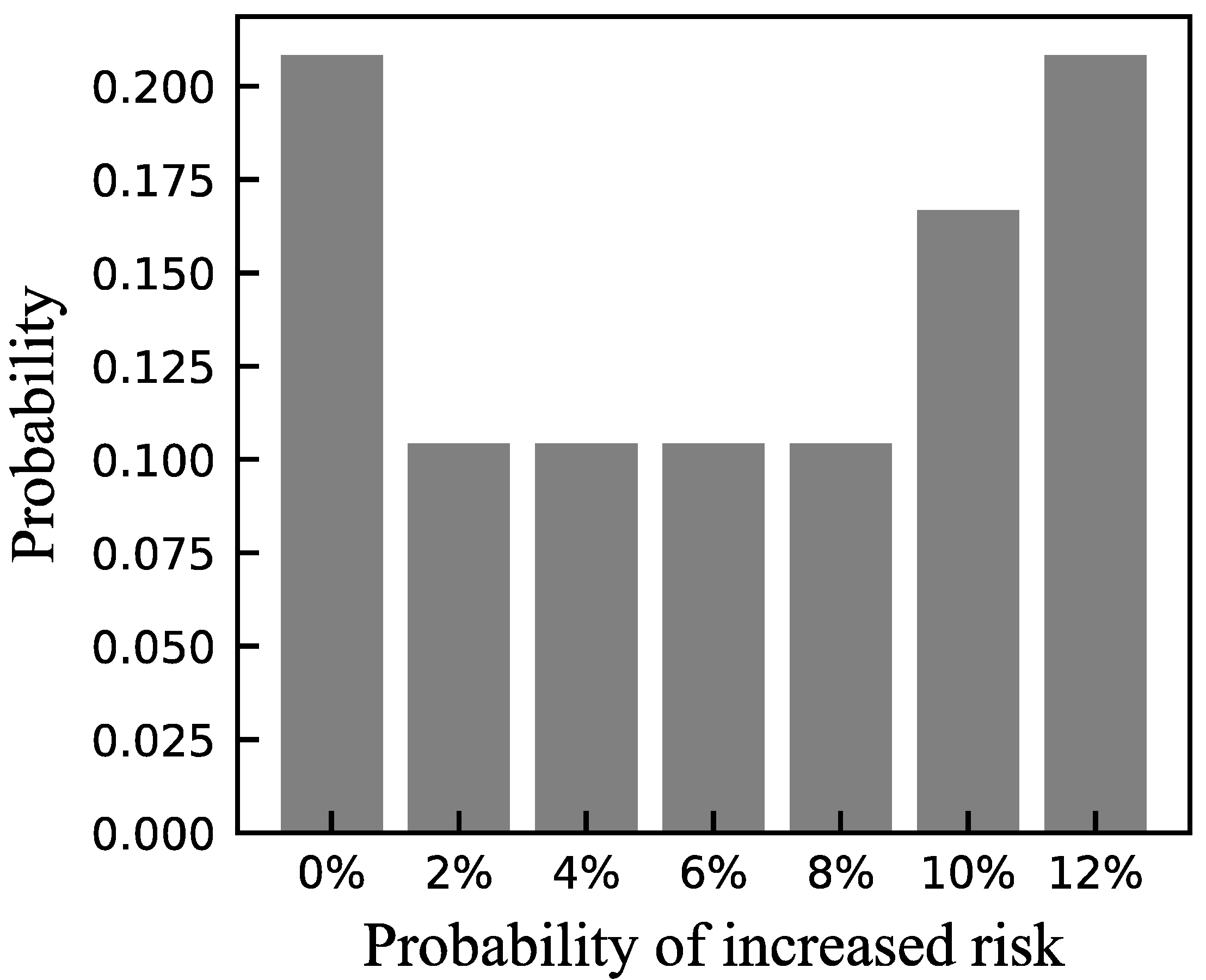
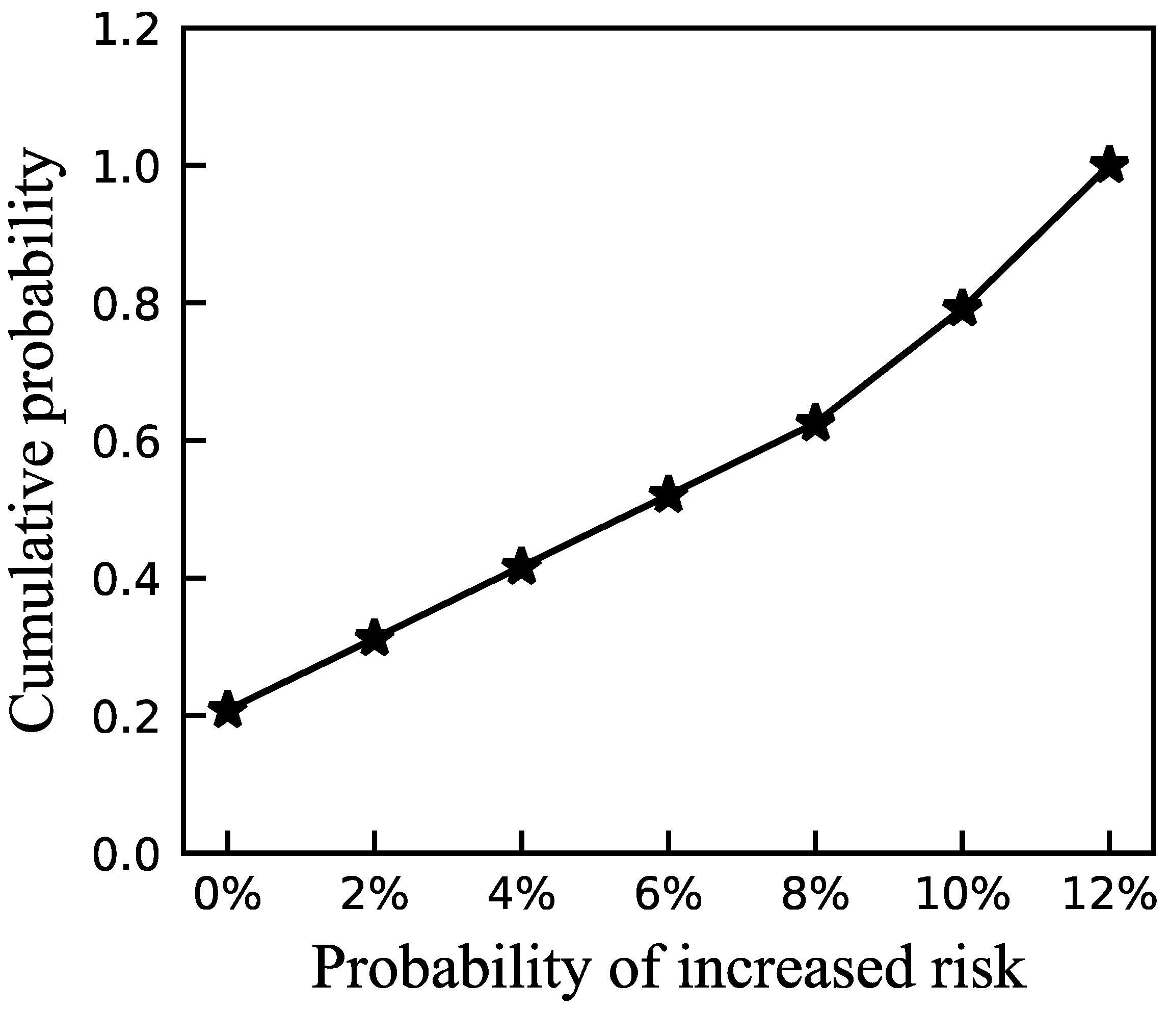
Referring to the descriptive term of the IPCC probability results (Table 1), it was concluded that the chance of this example dike was “very likely”. Figure 3 and Figure 4 show the probability distribution and cumulative distribution of the increased risk, respectively. The top three of the increased risk were 0%, 12%, and 10%, and the cumulative probability from 10% to 12% was 37.5%. The occurrence probability was relatively high, which was different from the result “very likely”. Actually, the expected value of 6.25% of structure failure cannot be accepted for flood defense. The two conclusions from cumulative cure and the expected value had the same meanings, indicating that a risk exists. Hence, the probabilistic result of IPCC was not suitable for the dikes perfectly. Developing a similarly descriptive term for dikes is an urgent task for hydraulic experts.
4. Summary and Conclusions
Based on the influence diagram, this paper proposed a risk assessment method for dikes with a risk chain model. We summarized the common risk resources that affect the safety of dikes based on general experiences. The relationships between the different risk nodes were also deduced. The whole process of risk assessment was displayed by taking an example of a hypothesis dike. The probability of dike damage was 6.25%, illustrating that the chance of dike damage is “very likely” according to the descriptive term proposed by the Intergovernmental Panel on Climate Change (IPCC). The advantages of the proposed method are summarized as follows.
(1) All the analytical risk factors and non-analytical risk factors can theoretically be integrated into the influence diagram. The risk resources in Table 2 are only the common ones. The other risk resources can be further added as a supplement when this method is used to evaluate different dikes.
(2) This method is based on fuzzy mathematics and uses the membership degree function to describe the uncertainty of the analytical risk factors and non-analytical factors, which is more prone to reality.
(3) The different failure modes can be considered during the process of risk assessment at the same time.
(4) The risk assessment is obtained as a probabilistic result, which enables an intuitive perception of dike safety. We can provide reasonable suggestions for the engineering management and regular maintenance of dikes.
Expected for the risk assessment of dikes, the risk chain model and fuzzy influence diagram method can be applied to other hydraulic structures and geotechnical engineering. To obtain more accurate assessment results in engineering applications, more comprehensive risk sources should be selected, and field surveys or/and tests should be conducted to obtain real engineering data for calculation.
Author Contributions
Conceptualization, Q.Z.; formal analysis, X.W. and R.T.; funding acquisition, Q.Z.; methodology, X.W. and X.X.; writing original-draft, X.W.; writing review and editing, X.G. All authors have read and agreed to the published version of the manuscript.
Funding
This research was funded by the National Natural Science Foundation of China (No. 12002118); the Fundamental Research Funds for the Central Universities (No. 2019B65814); Postgraduate Research & Practice Innovation Program of Jiangsu Province (No. SJKY19_0422); the National Key Research and Development Program of China (No. 2017YFC1502603).
Institutional Review Board Statement
This study did not require ethical approval.
Informed Consent Statement
Informed consent was obtained from all subjects involved in the study.
Data Availability Statement
No new data were created or analyzed in this study.
Acknowledgments
The author Xiaobing Wang also gratefully acknowledges the support from China Scholarship Council (No. 202006710049).
Conflicts of Interest
The authors declare no conflict of interests.
References
- Ministry of Water Resources, People’s Republic of China. 2019 Statistic Bulletin on China Water Activities; Water and Power Press: Beijing, China, 2019.
- Mouri, G.; Minoshima, D.; Golosov, V.; Chalov, S.; Seto, S.; Yoshimura, K.; Nakamura, S.; Oki, T. Probability assessment of flood and sediment disasters in Japan using the Total Runoff-Integrating Pathways model. Int. J. Disaster Risk Reduct. 2013, 3, 31–43. [Google Scholar] [CrossRef] [Green Version]
- Marijnissen, R.; Kok, M.; Kroeze, C.; Loon-Steensma, J. Re-evaluating safety risks of multifunctional dikes with a probabilistic risk framework. Nat. Hazards Earth Syst. Sci. 2019, 19, 737–756. [Google Scholar] [CrossRef] [Green Version]
- Balistrocchi, M.; Moretti, G.; Ranzi, R.; Orlandini, S. Failure probability analysis of levees affected by mammal bioerosion. Water Resour. Res. 2021, 57, e2021WR030559. [Google Scholar] [CrossRef]
- Agbaje, S.; Zhang, X.; Ward, D.; Dhimitri, L.; Patelli, E. Spatial variability characteristics of the effective friction angle of Crag deposits and its effects on slope stability. Comput. Geotech. 2022, 141, 104532. [Google Scholar] [CrossRef]
- Mao, C.X. Embankment Manual; Water and Power Press: Beijing, China, 2009. [Google Scholar]
- Xie, J.B.; Sun, D.Y. Model for analysis on reliability of levee overtopping and its application. Water Resour. Hydropower Eng. 2011, 42, 40–45. [Google Scholar]
- Sharp, J.A.; Mcanally, W.H. Numerical modeling of surge overtopping of a levee. Appl. Math. Model. 2012, 36, 1359–1370. [Google Scholar] [CrossRef] [Green Version]
- Yuan, S.Y.; Tang, H.W.; Li, L.; Pan, Y.; Amini, F. Combined wave and surge overtopping erosion failure model of HPTRM levees: Accounting for grass-mat strength. Ocean Eng. 2015, 109, 256–269. [Google Scholar] [CrossRef] [Green Version]
- Saladdin, M.; O’Sullivan, J.; Abolfathi, S.; Dong, S.; Pearson, J. Distribution of individual wave overtopping volumes on a sloping structure with a permeable foreshore. Coast. Eng. Proc. 2020, 36, 54. [Google Scholar] [CrossRef]
- Dong, S.; Abolfathi, S.; Salauddin, M.; Pearson, J.M. Spatial distribution of wave-by-wave overtopping at vertical seawalls. Coast. Eng. Proc. 2020, 36, 17. [Google Scholar] [CrossRef]
- Dong, S.; Abolfathi, S.; Salauddin, M.; Pearson, J.M. Spatial distribution of wave-by-wave overtopping behind vertical seawall with recurve retrofitting. Ocean Eng. 2021, 238, 109674. [Google Scholar] [CrossRef]
- Dong, S.; Salauddin, M.; Abolfathi, S.; Pearson, J. Wave impact loads on vertical seawalls: Effects of the geometrical properties of recurve retrofitting. Water 2021, 12, 2849. [Google Scholar] [CrossRef]
- Salauddin, M.; O’Sullivan, J.J.; Abolfathi, S.; Peng, Z.; Dong, S.; Pearson, J.M. New insights in the probability distributions of wave-by-wave overtopping volumes at vertical breakwaters. Sci. Rep. 2022, 12, 16228. [Google Scholar] [CrossRef]
- Guo, Y.; Zhu, D.; Zhang, F.; Lei, G.H.; Qiu, H.Y. Stability analysis of three-dimensional slopes under water drawdown conditions. Can. Geotech. J. 2014, 51, 1355–1364. [Google Scholar] [CrossRef]
- Yeganeh-Bakhtiary, A.; Houshangi, H.; Hajivalie, F.; Abolfathi, S. A numerical study on hydrodynamics of standing waves in front of caisson breakwaters with WCSPH model. Coast. Eng. J. 2017, 59, 1750005. [Google Scholar] [CrossRef] [Green Version]
- Guo, C.Y.; Li, D.Q.; Cao, Z.J.; Gao, G.H.; Tang, X.S. Efficient reliability sensitivity analysis for slope stability in spatial variable soils. Rock Soil Mech. 2018, 39, 2203–2210. [Google Scholar] [CrossRef]
- Wang, X.B.; Xia, X.Z.; Zhang, Q. Reliability Analysis on Anti-sliding Stability of Levee Slope Based on Orthogonal Test and Neural Network. J. Yangtze River Sci. Res. Inst. 2019, 36, 89–93. [Google Scholar] [CrossRef]
- Yeganeh-Bakhtiary, A.; Houshangi, H.; Abolfathi, S. Lagrangian two-phase flow modeling of scour in front of vertical breakwater. Coast. Eng. J. 2020, 62, 252–266. [Google Scholar] [CrossRef]
- Wang, Z.F.; Zhang, Z.Q.; Yang, G.S. Risk calculation model for flood levee structure. Shui Li Xue Bao 1998, 7, 64–67. [Google Scholar]
- Stark, T.D.; Jafari, N.H.; Leopold, A.L.; Brandon, T.L. Soil compressibility in transient unsaturated seepage analyses. Can. Geotech. J. 2014, 51, 858–868. [Google Scholar] [CrossRef]
- Ni, X.D.; Zhu, C.M.; Wang, Y. Analyzing the behavior of seepage deformation by three-dimensional coupled continuum-discontinuum methods. China Civ. Eng. J. 2015, 48, 159–165. [Google Scholar]
- Perlea, M.; Ketchum, E. Impact of non-analytical factors in geotechnical risk assessment of levees. In Geo-Risk, Risk Assessment and Management; American Society of Civil Engineers: Atlanta, GA, USA, 2011; pp. 1073–1081. [Google Scholar] [CrossRef]
- Song, Z.P.; Guo, D.S.; Xu, T.; Hua, W.X. Risk assessment model in TBM construction based on nonlinear fuzzy analytic hierarchy process. Rock Soil Mech. 2021, 42, 1424–1433. [Google Scholar] [CrossRef]
- Wang, Y.J.; Zhang, C.H.; Jin, F.; Zhang, W.H.; Wu, C.Y.; Ren, D.C. Research and application of comprehensive safety model and risk judgement system of embankment engineering. J. Nat. Disasters 2012, 21, 101–108. [Google Scholar]
- Gu, C.S.; Wang, Z.L.; Liu, C.D. Experts’ weight model assessing embankment safety. Rock Soil Mech. 2006, 27, 2099–2104. [Google Scholar]
- Wang, T.; Liao, B.C.; Ma, X.; Fang, D.P. Using Bayesian network to develop a probability assessment approach for construction safety risk. China Civ. Eng. J. 2010, 43, 384–391. [Google Scholar]
- Li, W.S.; Qin, X.Y.; Li, F.; Zhou, B. Analysis on probability of Stock Ammunition Accidents Based on FID. China Saf. Sci. J. 2009, 19, 62–69. [Google Scholar]
- Howard, R.A.; Matheson, J.E. Influence diagrams. Decis. Anal. 2005, 2, 127–143. [Google Scholar] [CrossRef]
- Yu, M. EPC Risk Identification and Analysis of Overseas Nuclear Power Project and Based on Risk Chain and Risk Map. Nucl. Sci. Eng. 2019, 39, 155–163. [Google Scholar]
- Xu, S.Y. Study on Construction Security Risk Assessment for Power Transmission Projection Based on Fuzzy Influence Diagram; Southeast University: Nanjing, China, 2016. [Google Scholar]
- Quan, J.; Huang, J.M.; Zhang, S.B.; Zeng, X.Y. Method of Risk Identification and Analysis Based on Risk Chain and Maps: A Case Study of an Overseas EPC Electric Power Project. Energy Constr. 2014, 1, 101–108. [Google Scholar]
- Quan, J.; Huang, J.M.; Zhang, S.B.; Zeng, X.Y. Method of Risk Qualitative Assessment Based on Risk Chain and Fuzzy Influence Diagrams: A Case Study of an Overseas EPC Electric Power project. South Energy Constr. 2016, 3, 63–69. [Google Scholar]
- Zhang, K.; Ge, L.; Wang, C.X.; Dai, F. Information Security Risk Assessment Based on Fuzzy Influence Diagram. J. Zhengzhou Univ. (Eng. Sci.) 2008, 29, 35–38. [Google Scholar]
- Lin, S.; Lin, W.Y. Fuzzy Influence Diagrams Method and Risk Evaluation. J. Tianjin Univ. Technol. 2005, 21, 73–77. [Google Scholar]
- Cheng, T.X.; Wang, P.; Zhang, W.B. Investigation on Fuzzy Influence Diagrams Evaluation Algorithm. J. Syst. Eng. 2004, 19, 177–182. [Google Scholar]
- Patt, A.G.; Schrag, D.P. Using specific language to describe risk and probability. Clim. Change 2003, 61, 17–30. [Google Scholar] [CrossRef]
Figure 1.
The risk chain structure.

Figure 2.
The fuzzy diagram.

Figure 3.
The distribution of the risk results.

Figure 4.
The cumulative probability of risk results.


Table 1.
The probabilistic result of IPCC.
| Probability Range | Descriptive Term |
|---|---|
| <1% | Extremely unlikely |
| 1~10% | Very unlikely |
| 10~33% | Unlikely |
| 33~66% | Medium likelihood |
| 66~90% | Likely |
| 90~99% | Very likely |
| >99% | Virtually certain |
Table 2.
The state and frequency of risk nodes.
| Nodes | The Potential Risk State | The Frequency |
|---|---|---|
| Flooding | big | low |
| middle | medium | |
| small | high | |
| Illegal operation | big | low |
| middle | medium | |
| small | high | |
| Low skills | big | low |
| middle | medium | |
| small | high | |
| Reduced cohesion | big | low |
| middle | high | |
| small | medium | |
| Increase of water content | big | medium |
| middle | low | |
| small | high | |
| Void ratio change | big | low |
| middle | medium | |
| small | high | |
| Friction angle change | big | low |
| middle | high | |
| small | medium | |
| …… | …… | …… |
Table 3.
The fuzzy relationship of different risk nodes.
| Relationship between Different Nodes | Relationship Description | |
|---|---|---|
| The Degree of Change in Disadvantage for the Risk Nodes | The Results Corresponding to the Degree of Change of the Risk Nodes | |
| Flooding → higher water level | big, middle, and small, respectively | Increase max, increase medium, increase min, respectively |
| Illegal operation → reduced drainage capacity | big, middle, and small, respectively | Increase max, increase medium, increase min, respectively |
| Low skills → reduced drainage capacity | big, middle, and small, respectively | Increase max, increase medium, increase min, respectively |
| Reduced cohesion → dike body damage | big, middle, and small, respectively | Increase max, increase medium, increase min, respectively |
| Water content → dike body damage | big, middle, and small, respectively | Increase max, increase medium, increase min, respectively |
| Reduced cohesion → dike foundation damage | big, middle, and small, respectively | Increase max, increase medium, increase min, respectively |
| water content → dike foundation damage | big, middle, and small, respectively | Increase max, increase medium, increase min, respectively |
| Void ratio → dike body damage | big, middle, and small, respectively | Increase max, increase medium, increase min, respectively |
| Friction angel → dike foundation damage | big, middle, and small, respectively | Increase max, increase medium, increase min, respectively |
| Void ratio → dike foundation damage | big, middle, and small, respectively | Increase max, increase medium, increase min, respectively |
| Friction angle → dike foundation damage | big, middle, and small, respectively | Increase max, increase medium, increase min, respectively |
| Higher water level → overtopping | Increase max, medium, min, respectively | Increase max, increase medium, increase min, respectively |
| Reduced drainage → overtopping | Increase max, medium, min, respectively | Increase max, increase medium, increase min, respectively |
| Damage of dike body → seepage | Increase max, medium, min, respectively | Increase max, increase medium, increase min, respectively |
| Damage of dike foundation → seepage | Increase max, medium, min, respectively | Increase max, increase medium, increase min, respectively |
| Damage of dike body → scouring | Increase max, medium, min, respectively | Increase max, increase medium, increase min, respectively |
| Damage of dike foundation → scouring | Increase max, medium, min, respectively | Increase max, increase medium, increase min, respectively |
| Overtopping → dike failure | Increase max, medium, min, respectively | Increase max, increase medium, increase min, respectively |
| Seepage → dike failure | Increase max, medium, min, respectively | Increase max, increase medium, increase min, respectively |
| Scouring → dike failure | Increase max, medium, min, respectively | Increase max, increase medium, increase min, respectively |
Take the “Flooding → higher water level” and “Higher water level → overtopping” as examples to illustrate Table 3. When the flooding is big, middle, and small, it can cause an increase in water level to maximum, medium, and minimum, respectively. When the increase of higher water level is maximum, medium, and minimum, it can cause a degree of overtopping to maximum, medium, and minimum, respectively.
Disclaimer/Publisher’s Note: The statements, opinions and data contained in all publications are solely those of the individual author(s) and contributor(s) and not of MDPI and/or the editor(s). MDPI and/or the editor(s) disclaim responsibility for any injury to people or property resulting from any ideas, methods, instructions or products referred to in the content. |
© 2022 by the authors. Licensee MDPI, Basel, Switzerland. This article is an open access article distributed under the terms and conditions of the Creative Commons Attribution (CC BY) license (https://creativecommons.org/licenses/by/4.0/).
Share and Cite
MDPI and ACS Style
Wang, X.; Xia, X.; Teng, R.; Gu, X.; Zhang, Q. Risk Assessment of Dike Based on Risk Chain Model and Fuzzy Influence Diagram. Water 2023, 15, 108. https://doi.org/10.3390/w15010108
AMA Style
Wang X, Xia X, Teng R, Gu X, Zhang Q. Risk Assessment of Dike Based on Risk Chain Model and Fuzzy Influence Diagram. Water. 2023; 15(1):108. https://doi.org/10.3390/w15010108
Chicago/Turabian StyleWang, Xiaobing, Xiaozhou Xia, Renjie Teng, Xin Gu, and Qing Zhang. 2023. "Risk Assessment of Dike Based on Risk Chain Model and Fuzzy Influence Diagram" Water 15, no. 1: 108. https://doi.org/10.3390/w15010108
Note that from the first issue of 2016, this journal uses article numbers instead of page numbers. See further details here.