Impact of Geometrical Features on Solute Transport Behavior through Rough-Walled Rock Fractures

Abstract

The solute transport in the fractured rock is dominated by a single fracture. The geometric characteristics of single rough-walled fractures considerably influence their solute transport behavior. According to the self-affinity of the rough fractures, the fractal model of single fractures is established based on the fractional Brownian motion and the successive random accumulation method. The Navier–Stokes equation and solute transport convective-dispersion equation are employed to analyze the effect of fractal dimension and standard deviation of aperture on the solute transport characteristics. The results show that the concentration front and streamline distribution are inhomogeneous, and the residence time distribution (RTD) curves have obvious tailing. For the larger fractal dimension and the standard deviation of aperture, the fracture surface becomes rougher, aperture distribution becomes more scattered, and the average flow velocity becomes slower. As a result, the average time of solute transport is a power function of the fractal dimension, while the time variance and the time skewness present a negative linear correlation with the fractal dimension. For the standard deviation of aperture, the average time exhibits a linearly decreasing trend, the time variance is increased by a power function, and the skewness is increased logarithmically.

1. Introduction

Solute transport analysis in fractured rock is critical in many applications, such as geological storage of nuclear waste [1], landfill [2] and pollutant migration with groundwater [3]. Due to the geological actions and engineering disturbances, the fracture geometry involving aperture distribution and surface roughness is commonly heterogeneous and anisotropic [4,5], which significantly influences the solute transport characteristics of a rock mass.

The single fracture is a basic component unit of fractured rock, which is the theoretical basis of solute transport in complicated rock [6,7,8,9,10,11]. Many studies have been conducted on the parallel plates of a single fracture. For instance, Edson and Thomas [12] have preliminarily emphasized that the average aperture and the standard deviation of aperture have an important influence on the solute transport breakthrough curve using a three-dimensional parallel version of the test and numerical simulation. Yu and Lei [13] combined the smooth parallel plate model and the local cubic theorem to transform the three-dimensional model into a two-dimensional plane model. The results show that the concentration front becomes more heterogeneous when the fracture aperture decreases. However, the surface roughness and aperture distribution of natural fractures are random and irregular [14,15]. To investigate the relationship between the solute transport characteristics and the heterogeneous distribution of aperture and surface roughness, Wang and Zhou [16] carried out a numerical simulation of a single fracture with different fracture roughness, and the results showed that the concentration front of a rough fracture has obvious unevenness and anisotropy. Jeong and Song, Zou et al., and Stoll et al. [17,18,19] studied the relationship between the solute transport characteristics and normal pressure by numerical simulation and indicated that fracture roughness and normal stress have a great influence on solute transport. From the solute transport simulations, with respect to the different fracture geometric characteristics, [20] found that the solute transport breakthrough curve and residence time distribution curve have obvious early arrival and long tail phenomena. Wang et al. [21] analyzed the effects of roughness and normal pressure on fluid flows and solute transport characteristics in three-dimensional rough fractures under constant normal stiffness boundary conditions, and the results showed that solute dispersion transport behavior became more obvious with the increase of normal pressure and the Hurst value. However, the quantitative analysis of fracture geometry on solute transport characteristics is insufficient, and there are few studies considering the influence of the standard deviation of aperture on solute transport.

According to the above studies, the aperture and roughness can lead to an uneven distribution of concentration fronts and streamlines, and the solute transport breakthrough curve and residence time curve produce early arrival and long tail. In order to describe these types of uneven changes quantitatively, most scholars adopt the fastest arrival time, median time and peak time to analyze the changes, and the influence mechanism is explained by comparing the variation in the residence time curve. For example, Hu et al. [22] adopted the fastest breakthrough time to quantitatively analyze the solute penetration curve, and the variation of the residence time distribution curve was used to describe the overall transport speed. Zou and Cvetkovic [23] used the fastest time, median time and peak time to describe the variation characteristics of the solute penetration curve. Wang et al. [24] used the solute penetration curve and residence time distribution curve to analyze the influence of different contact deformations on solute transport in fractures. Wang et al. [21] compared the mean and standard deviations of particle travel time under different normal pressures and fractal dimensions to analyze the variation of the Peclet value (ratio of convection rate to diffusion rate). It can be concluded that the fastest arrival time and peak concentration time are mainly used to express the distribution characteristics of the solute penetration curve, but they cannot reflect the speed of the overall transport. However, the question of how to quantify the asymmetric distribution and tailing characteristics for the residence time curve is still lacking in most previous studies. In order to address the above problems, the fractional Brownian motion and the successive random accumulation method are proposed to generate the self-affinity of the rough fractures. The Navier–Stokes equation and solute transport convective-dispersion equation are employed to simulate the solute transport process through single rough-walled fractures with different fractal dimensions and standard deviation, in which the average time, time variance and time skewness are used to quantify the overall solute transport speed, dispersion characteristics and tailing phenomenon, respectively. The relationships between the average time, time variance, time skewness and fracture roughness, and aperture distribution are established.

2. Generation of Rough-Walled Fracture

Based on the self-affinity of the fracture surface, fractal geometry theory is employed to describe the irregular morphology of rough fractures [22,25,26]. In three-dimensional fractional Brownian motion, a single-valued continuous random function, z (x,y), is defined to represent the variation in the surface elevation in space. For the arbitrary distance, h, the steady-state increment (z(x + h,y) z(x,y)) or (z(x,y + h) z(x,y)) obeys the normal distribution with mean zero and variance δ². The self-affinity of a fractional Brownian motion increment can be stated as:

$$\{\begin{array}{l}\langle \left[z\left(x,y\right)-z\left(x+rh,y\right)\right]\rangle =0\\ \langle \left[z\left(x,y\right)-z\left(x,y+rh\right)\right]\rangle =0\end{array}$$

(1)

$$\{\begin{array}{l}\langle {\left[z\left(x,y\right)-z\left(x+rh,y\right)\right]}^2\rangle =r^{2\left(3-D\right)}\langle {\left[z\left(x,y\right)-z\left(x+h,y\right)\right]}^2\rangle \\ \langle {\left[z\left(x,y\right)-z\left(x,y+rh\right)\right]}^2\rangle =r^{2\left(3-D\right)}\langle {\left[z\left(x,y\right)-z\left(x,y+h\right)\right]}^2\rangle \end{array}$$

(2)

where <·> is the mathematical expectation, D is the fractal dimension, and r is the constant.

The variance is expressed as:

$${\delta }_{rh}^2=\{\begin{array}{l}\langle {\left[z\left(x,y\right)-z\left(x+rh,y\right)\right]}^2\rangle \\ \langle {\left[z\left(x,y\right)-z\left(x,y+rh\right)\right]}^2\rangle \end{array}$$

(3)

$${\delta }_h^2=\{\begin{array}{l}\langle {\left[z(x,y)-z\left(x+h,y\right)\right]}^2\rangle \\ \langle {\left[z(x,y)-z\left(x,y+h\right)\right]}^2\rangle \end{array}$$

(4)

Combining F Equations (3) and (4) gives:

$${\delta }_{rh}^2=r^{2\left(3-D\right)}{\delta }_h^2\Rightarrow {\delta }_{rh}=r^{3-D}{\delta }_h$$

(5)

where ${\delta }_{rh}^2$ and ${\delta }_h^2$ are the variance subjects to the elevation increments rh and h, respectively.

According to the successive random addition method, in each step of subdivision, the fracture surface is divided into the square subdomain, and the center points and midpoints are linearly interpolated by averaging the elevation of the neighbor corner points. At the same time, a random elevation from the normal distribution $N\left(0,{\Delta }_n^2\right)$ is added to each point and

$${\Delta }_n^2={\delta }_0^2\left(1-2^{4-2D}\right)/{\left(2^{2\left(3-D\right)}\right)}^n$$

to guarantee the self-affinity Equation (5). In this way, the lower surface of the fracture is quantified by z₁ (x,y), and the upper fracture surface z₂ (x,y) can be obtained by the shear displacement method from Wang et al. (1988):

$$z_2\left(x,y\right)=z_1\left(x+x_d,y+y_d\right)+u$$

(6)

where $\left(x_d,y_d\right)$ is the r shear displacement.

The fracture aperture function b(x,y) can be expressed as:

$$b\left(x,y\right)=\{\begin{array}{cc}{z}_2\left(x,y\right)-z_1\left(x,y\right)& {\mathrm{if} \mathrm{z}}_2\left(x,y\right)>z_1\left(x,y\right)\\ 0& \mathrm{otherwise}\end{array}$$

(7)

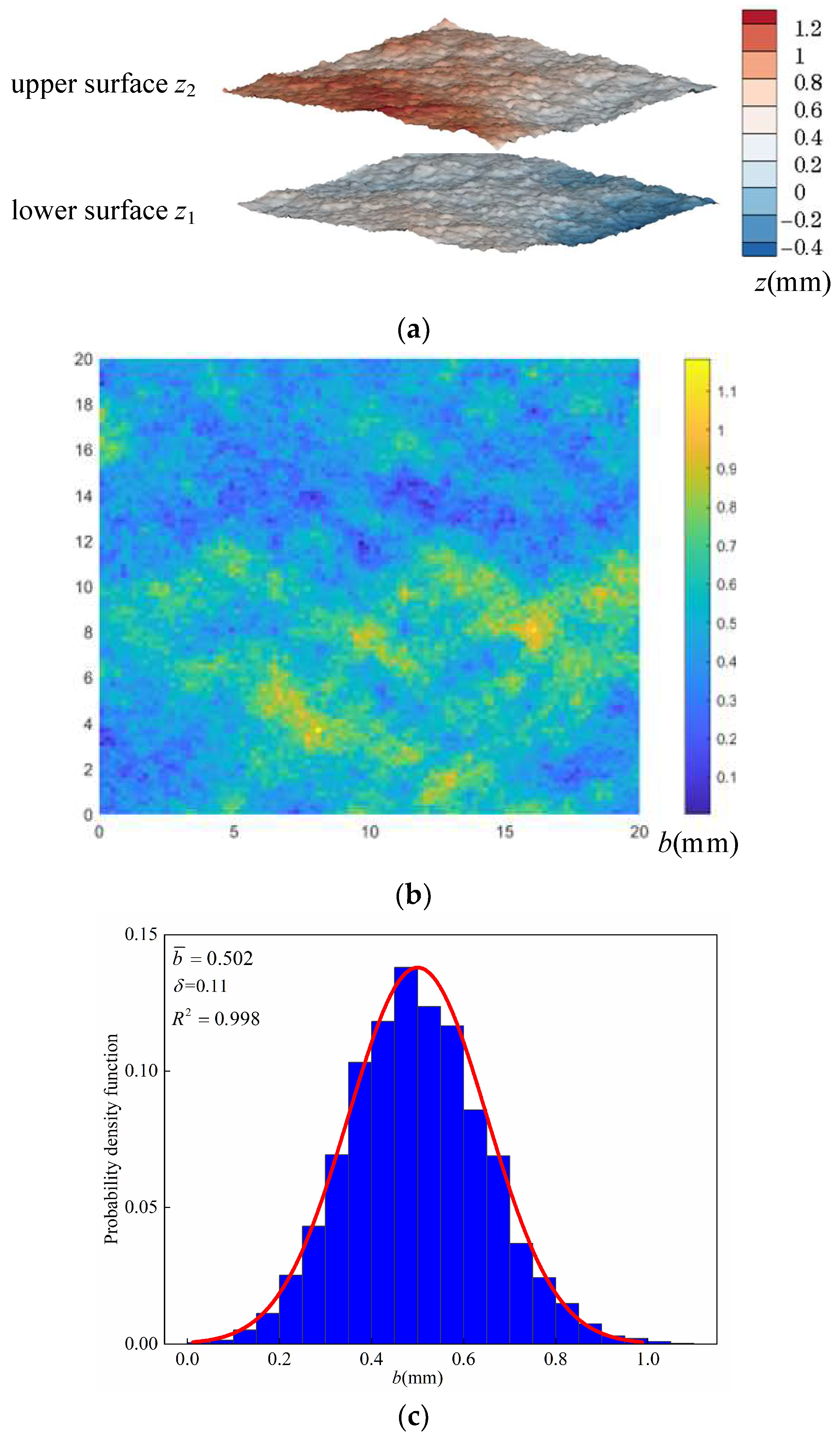
A typical example of fracture generation and its aperture distribution associated with the fractal dimension D = 2.5, mean aperture $\overline{b}$ = 0.5 mm and standard deviation δ = 0.11 mm are shown in Figure 1. As shown in Figure 1c, the aperture distribution from numerical generation is obtained as $\overline{b}$ = 0.502 mm and δ = 0.11 mm, which are close to the input values. Therefore, the successive random addition method is valid for generating rough-walled fractures.

3. Solute Transport Model in Rough Fracture

For the isothermal, incompressible, and homogenous single Newtonian steady flow, the fluid motion in a single rough-walled fracture can be solved using the Navier-Stokes and continuity Equations [27,28]:

$$\nabla \cdot \mathit{u}=0$$

(8)

$$\rho \left(\mathit{u}\cdot \nabla \right)\mathit{u}-\mu {\nabla }^2\mathit{u}=-\nabla p$$

(9)

where ρ, u, P, and µ are the fluid density, velocity vector, fluid pressure and dynamic viscosity, respectively.

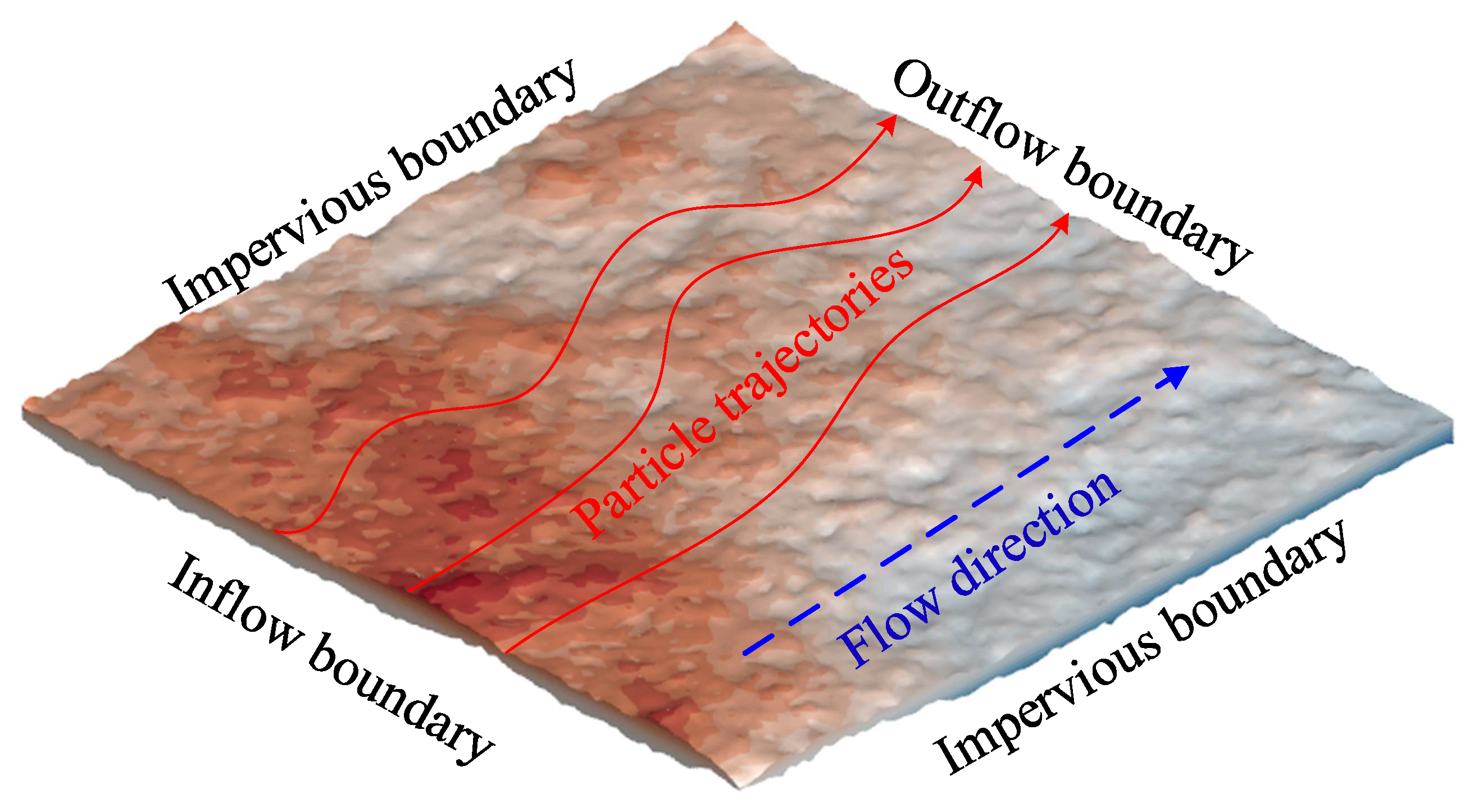
For the numerical simulations, the fracture surfaces are considered non-slip boundaries. As shown in Figure 2, the fluid flow occurs under the hydraulic gradient from the inflow boundary on the left side to the outflow boundary on the right side; the residual boundaries are specified as impermeable.

As demonstrated by Bodin et al. [29,30], the physical mechanism of solute transport in fractured rock mass includes advection, dispersion and diffusion, diffusion from a fracture to a matrix in a matrix, fracture surface and matrix adsorption, radioactive decay and chemisorption. For simplicity, the solute transport behavior of the fractures is concentrated in the advection and dispersion. The advection and dispersion Equations of rough-walled fractures can be expressed as:

$$\frac{\partial C}{\partial t}=\frac{\partial }{\partial x}\left(D_{xx}\frac{\partial }{\partial x}+D_{xy}\frac{\partial }{\partial y}\right)+\frac{\partial }{\partial y}\left(D_{yx}\frac{\partial C}{\partial x}+D_{xx}\frac{\partial C}{\partial x}\right)-\frac{\partial }{\partial x}\left(C\cdot u_x\right)-\frac{\partial }{\partial x}\left(C\cdot u_y\right)$$

(10)

where C, u, t and D are the solute concentration, average velocity, time and diffusion coefficient, respectively.

The initial and boundary conditions yield:

$$C\left(x,y,z,0\right)=0$$

(11)

$${C_{\mathrm{in}}|}_{x=0,t>0}=C_1$$

(12)

$${\frac{\partial C}{\partial \mathit{n}}|}_{x=l,t\ge 0}=0$$

(13)

where L is the fracture length along the flow direction, and n is the normal outward vector to the boundary.

COMSOL Multiphysics is a multi-physical field coupling simulation software based on the finite element method. It is widely used in flow and solute transport simulations in fractured rock, and its reliability has been fully verified [22,25,31]. In this study, the fracture surfaces generated by successive random addition methods are exported into the dxf format and then imported into COMSOL to form a three-dimensional solid model of rough fracture by block cutting, as shown in Figure 2. The laminar flow module and dilute material transfer module are applied to analyze the flow and solute transport process through the three-dimensional rough fractures. In order to ensure the calculation accuracy, the number of rough fracture model elements is controlled at about 2.5 million.

4. Results and Analysis

4.1. Concentration Distribution

In order to investigate the effect of the fracture geometry on the solute behavior, the size of all the rough fracture models was fixed as 20 mm × 20 mm, and the mean aperture was 0.5 mm. The fractal dimension varied from 2.1 to 2.5, while the standard deviation ranged from 0.07 to 0.15. The total simulation time was 1500 s, the inflow boundary concentration was set as 1 mol/L, the dispersion coefficient was 2.03 × 10⁻⁹ m²/s, and the pressure difference between the inflow boundary and outflow boundary was 0.05Pa.

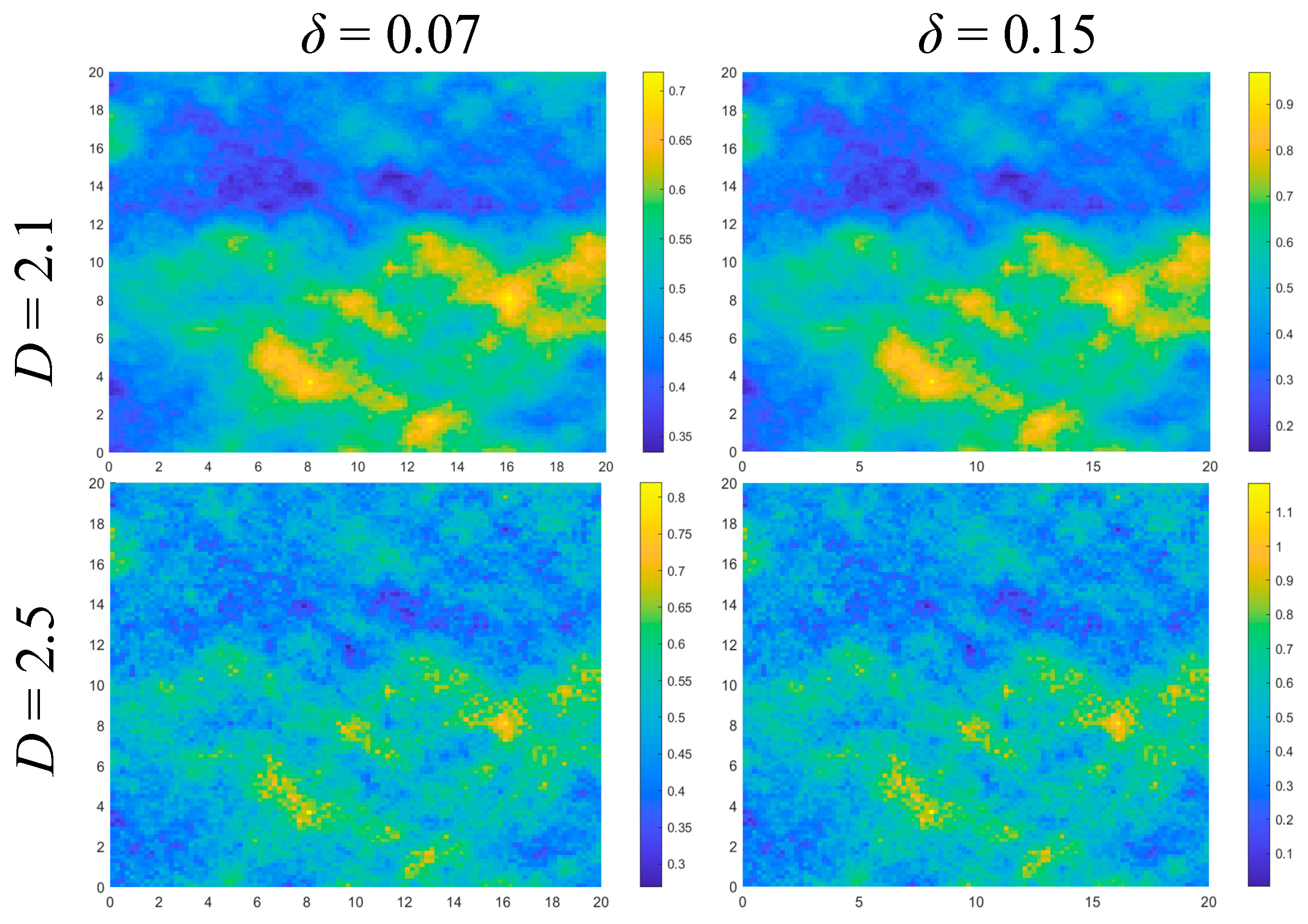
As shown in Figure 3, four groups of aperture distributions are presented with D = 2.1, 2.5, and δ = 0.07, 0.15, respectively. For D = 2.1 and δ = 0.07, the aperture distribution is compact, and the spatial variation is gentle, while for D = 2.5 and δ = 0.15, the aperture distribution is dispersed, and the spatial variation is drastic. The results show that, with the increase of the fractal dimension and standard deviation of aperture, the fracture surface becomes more rough-walled and fluctuated.

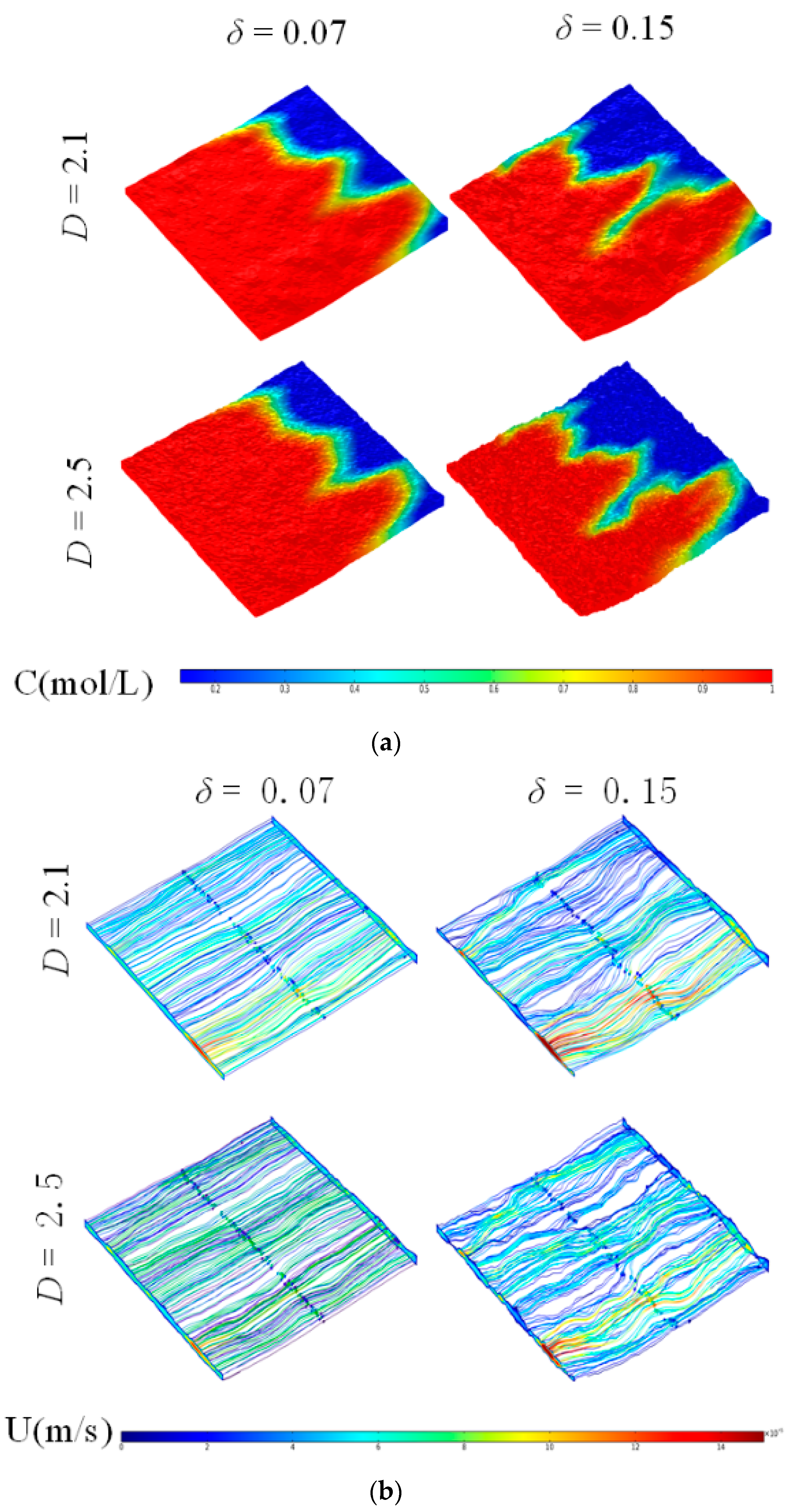
Corresponding to Figure 3, the concentration distribution and streamlined distribution of the four groups are shown in Figure 4. The distribution of the concentration fronts and streamlines is inhomogeneous. With the increase of the fractal dimension and standard deviation of fracture aperture, the streamlines turn to be more tortuous, and the flow distribution becomes more uneven, which leads to the enhancement of the inhomogeneity of the concentration front. The results show that the geometrical characteristics of rough fractures have an important effect on their solute transport characteristics.

4.2. Breakthrough Curve

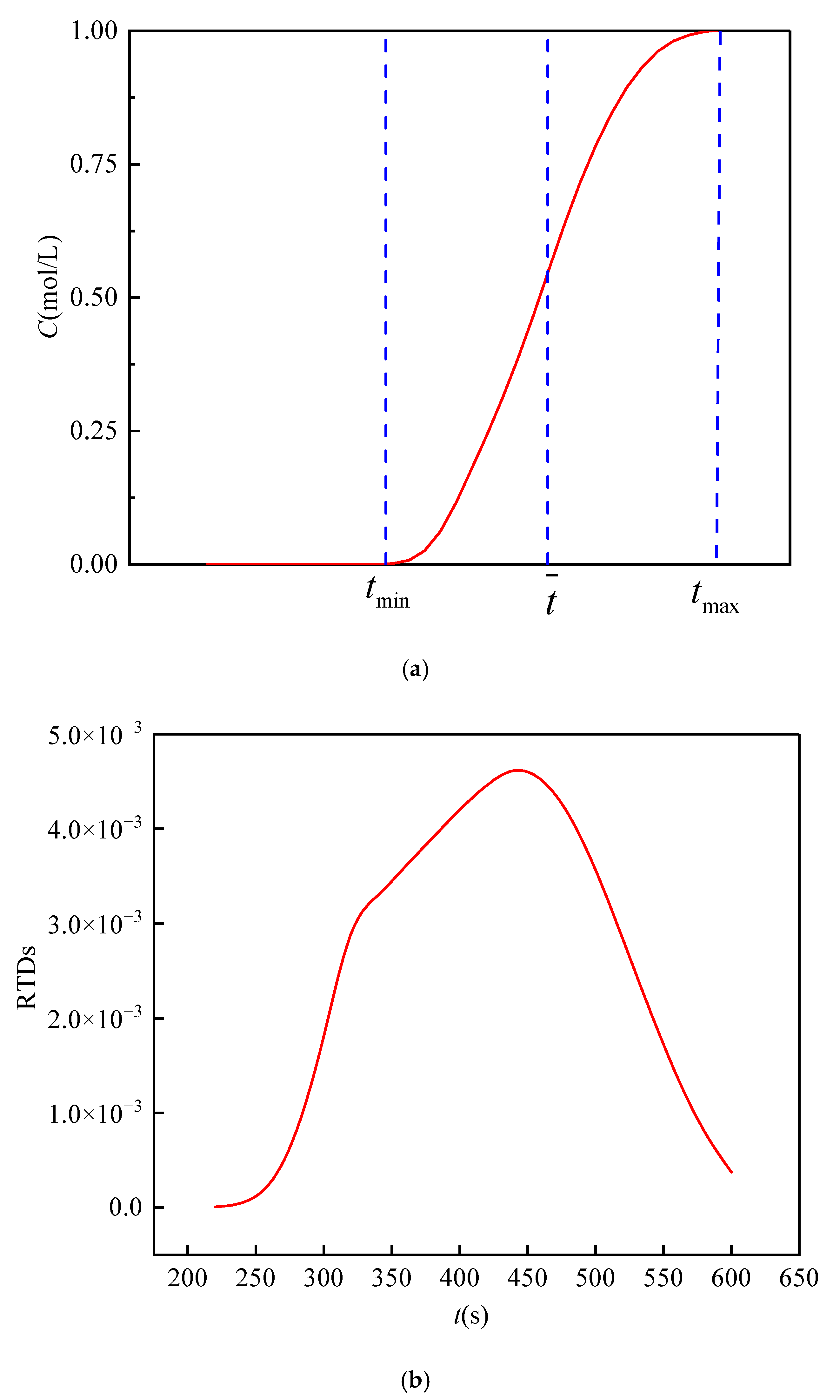
In order to quantify the influence of fracture geometry on solute transport behaviors, the average time $\overline{t}$, time variance $s^2$ and time skewness $s{k}_t$ are used to represent the speed, dispersion and tailing of solute transport, respectively. The solute transport breakthrough curve (BTC) and residence time distribution curve (RTD) are shown in Figure 5. The average time $\overline{t}$ of solute transport is calculated by selecting the fastest time $t_{\min }$ and the peak time $t_{\max }$ arriving at the outflow boundary as:

$$\overline{t}=\frac{{\displaystyle {\int }_{t_{\min }}^{t_{\max }}f\left(t\right)tdt}}{{\displaystyle {\int }_{t_{\min }}^{t_{\max }}f\left(t\right)dt}}$$

(14)

The time variance $s^2$ and time skewness $s{k}_t$ of the residence time distribution curve is calculated on the basis of average time:

$$s^2=\frac{{\displaystyle {\int }_{t_{\min }}^{t_{\max }}f\left(t\right){(t_i-\overline{t})}^{2}dt}}{{\displaystyle {\int }_{t_{\min }}^{t_{\max }}f\left(t\right)dt}}$$

(15)

$$s{k}_t=\frac{{\displaystyle {\int }_{t_{\min }}^{t_{\max }}f\left(t\right){(\frac{t_i-\overline{t}}{s})}^{3}dt}}{{\displaystyle {\int }_{t_{\min }}^{t_{\max }}f\left(t\right)dt}}$$

(16)

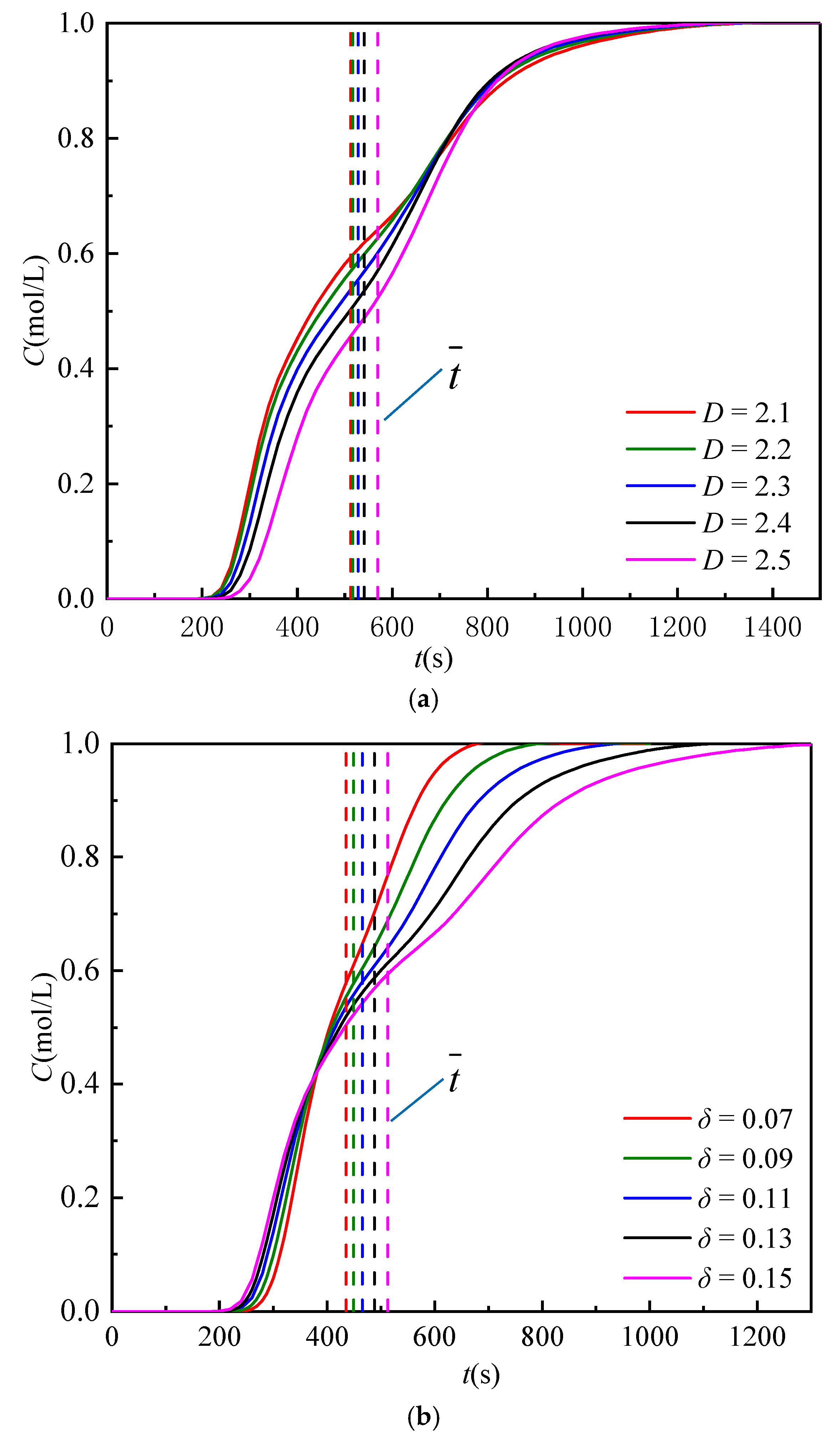
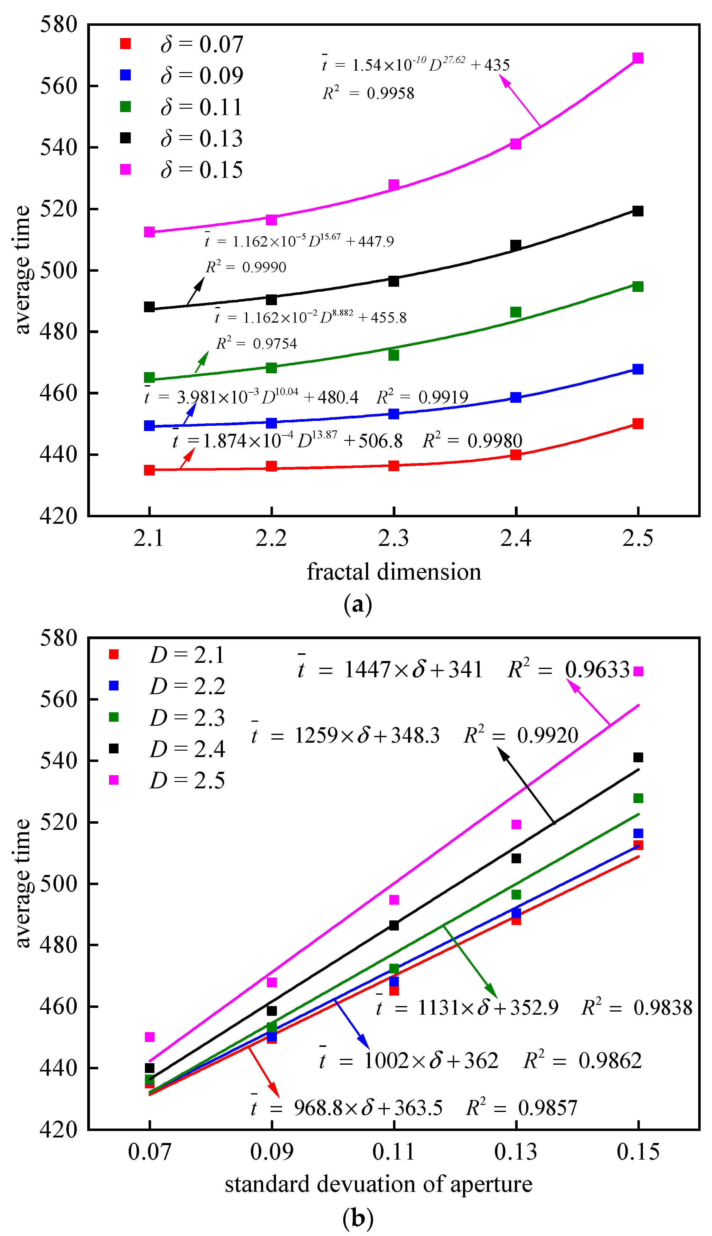
Figure 6 shows the breakthrough curve and average time of the solute transport from different fractal dimensions and the standard deviation of aperture. The average arrival time of solute transport increases with the growth of the fractal dimension and standard deviation of aperture. This is because the increase in fracture roughness makes the flow velocity slow and then leads to an increase in the average time of solute transport. As shown in Figure 7a, the average time increases nonlinearly with the increase of fractal dimension. The relationship between the average time and fractal dimension can be approximated by a power function as below:

$$\overline{t}=a_1{D}^{b_1}+c_1$$

(17)

As shown in Figure 7b, the average time increases linearly with the increase of the standard deviation of aperture. The relationship between the average time and standard deviation of aperture is described by:

$$\overline{t}=a_2\delta +b_2$$

(18)

where a, b and c are constants.

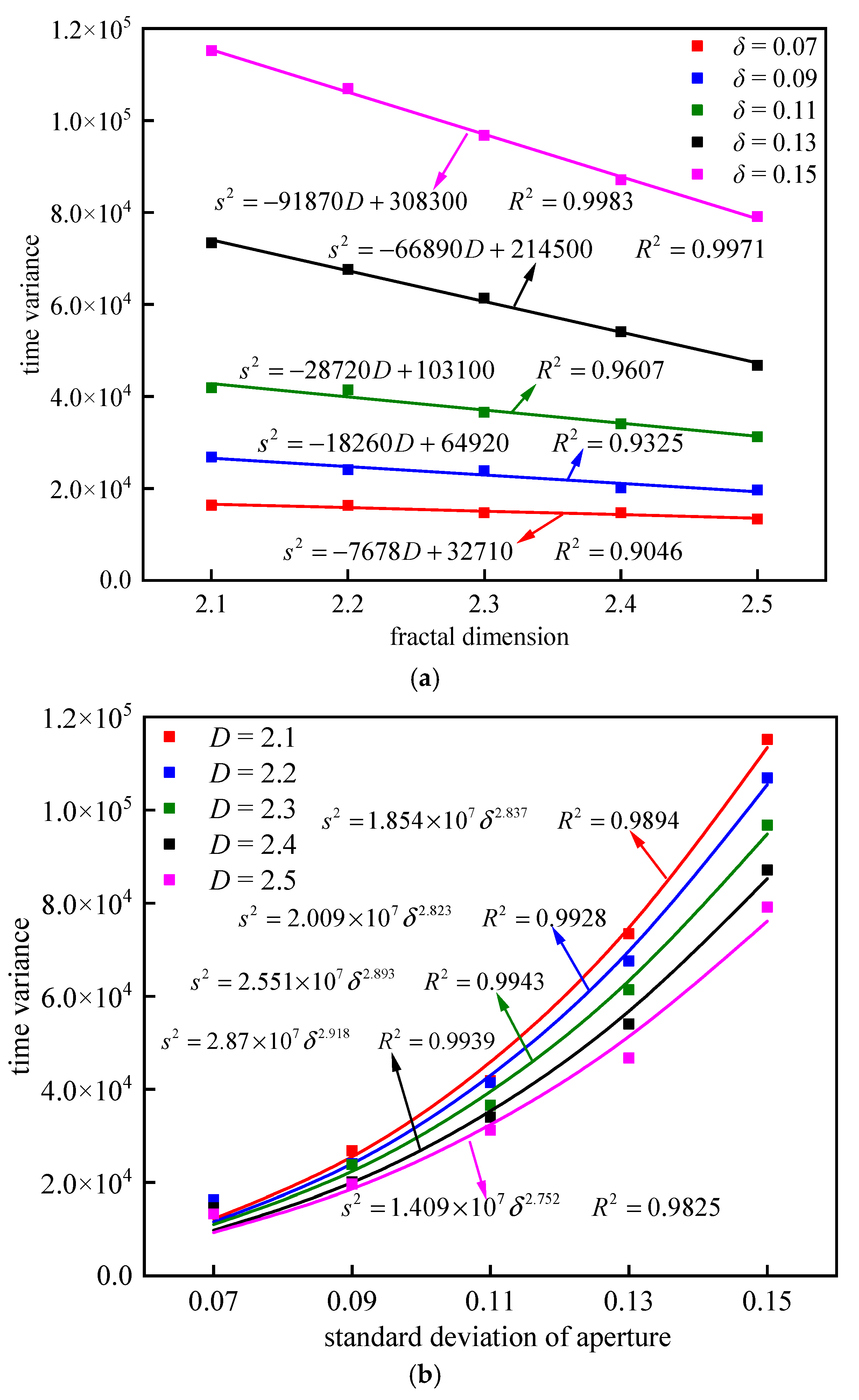
Figure 8 shows the time variance of solute transport from different fractal dimensions and the standard deviation of aperture. The time variance decreases with the increase of fractal dimension and increases with the increase of standard deviation, respectively. As shown in Figure 8a, with the increase of fractal dimension, the time variance linearly decreases. The relationship between time variance and fractal dimension can be expressed as:

$$s^2=a_{3}D+b_3$$

(19)

As shown in Figure 8b, with the increase of standard deviation of aperture, the time variance nonlinearly increases. The relationship between the time variance and standard deviation of aperture can be described by a power function:

$$s^2=a_4{\delta }^{b_4}$$

(20)

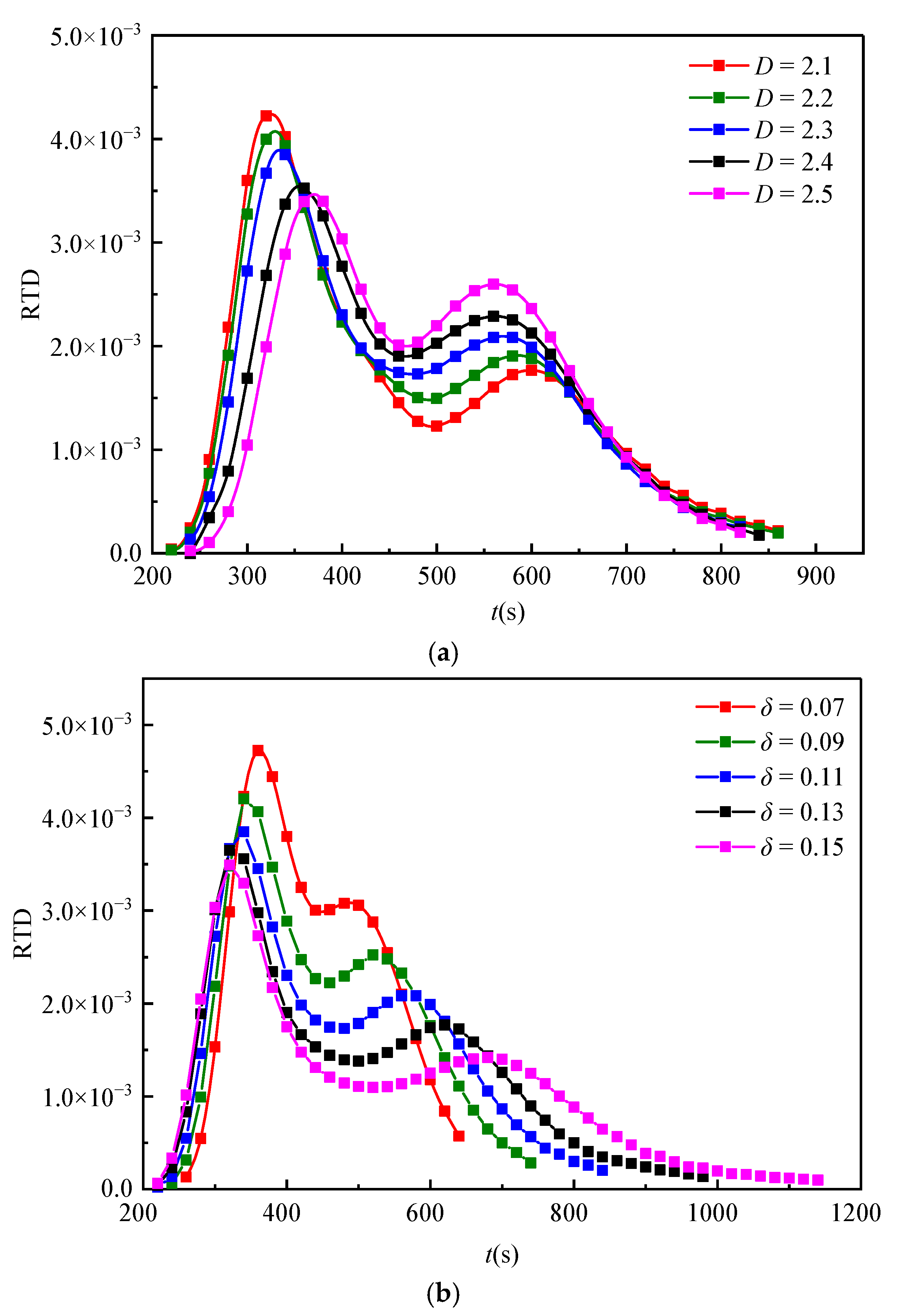
Figure 9 shows the RTD curves from different fractal dimensions and the standard deviation of aperture. The RTD curves are generally asymmetric and behave in a tailing manner. With the increase of fractal dimension, the RTD curves skew to the right. The increase of the standard deviation of aperture makes the right part of the RTD curves flatter.

As the fractal dimension increases, the fastest time $t_{\min }$ increases, and the peak time $t_{\max }$ decreases. However, the intermediate area of the RTD curves becomes narrow, indicating that a larger standard deviation can lead to a wide-ranging distribution of RTD curves. However, with the increase of the standard deviation of aperture, the preferential flow is more easily formed to decrease the fastest time $t_{\min }$ and increase the peak time $t_{\max }$. Therefore, the larger range of the time distribution results in a greater time variance.

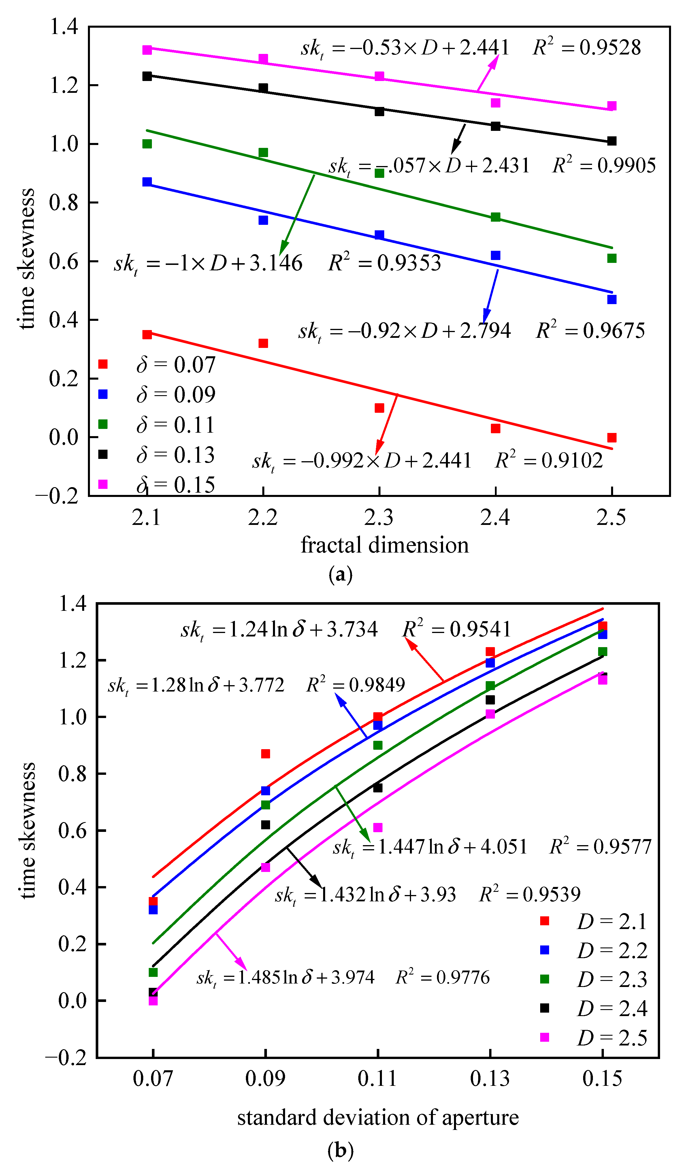
Figure 10 shows the variation of time skewness for different fractal dimensions and the standard deviation of aperture. With the increase of fractal dimension, the curve symmetry is enhanced, but the tailing and skewness decrease. For the increase of the standard deviation, the curve symmetry is weakened, but the trailing is more pronounced, and the skewness increases.

As shown in Figure 10a, the linear relationship between time skewness and the fractal dimension can be expressed as:

$$s{k}_t=a_{5}D+b_5$$

(21)

As shown in Figure 10b, the nonlinear relationship between time skewness and standard deviation can be stated as:

$$s{k}_t=a_6\ln \delta +b_6$$

(22)

5. Conclusions

The solute transport behavior through single fractures is greatly affected by the aperture distribution and surface roughness; a systematic approach is still required to quantify the asymmetric distribution and tailing characteristics of RTD curves with respect to the geometrical characteristics of single fractures. In order to evaluate the effect of fracture geometry on the solute transport behaviors, the rough-walled fractures are generated based on fractional Brownian motion and the successive random addition method. The Navier–Stokes and solute transport convective-dispersion equations are solved by the COMSOL software. The average time $\overline{t}$, time variance $s^2$ and time skewness $s{k}_t$ are obtained to describe the speed, dispersion and tailing of solute transport. The main conclusions are as follows:

(1)

The geometric model of rough-walled fractures is successfully generated by the successive random addition method, which can guarantee consistency between the output and input values. With the increased fractal dimension and standard deviation, the fracture roughness becomes larger, and the aperture distribution becomes more scattered, which can make the streamline more tortuous, the flow distribution more uneven, and the concentration front more inhomogeneous.

(2)

With the growth of fractal dimensions, the average time of solute transport increases nonlinearly, and the time variance decreases linearly, respectively. The RTD curve skews more to the right, and the middle region turns to be more concentrated. The curve symmetry is enhanced, the tailing degree is weakened, and the time skewness is decreased.

(3)

With the increase of the standard deviation, the average time and the time variance of solute transport increase linearly and nonlinearly, respectively. The right part of RTD curves turns to be flatter with a larger range of time distribution, and the tailing degree is enhanced. Therefore, the curve symmetry is weakened while the skewness is increased.

(4)

Based on the curve fitting, the average time of solute transport linearly increases with the standard deviation and the fractal dimension by the power function. The time variance has a linear decreasing relationship with fractal dimension and a power function increasing relationship with standard deviation. The time skewness has a linear decreasing relationship with fractal dimension and a logarithmic increasing relationship with standard deviation.

References

- Cassiraga, E.F.; Fernàndez-Garcia, D.; Gómez-Hernández, J.J. Performance assessment of solute transport upscaling methods in the context of nuclear waste disposal. Int. J. Rock Mech. Min. Sci. 2005, 42, 756–764. [Google Scholar] [CrossRef]
- Zhang, H.J.; Jeng, D.S.; Seymour, B.R.; Barry, D.A.; Li, L. Solute transport in partially-saturated deformable porous media: Application to a landfill clay liner. Adv. Water Resource. 2012, 40, 1–10. [Google Scholar] [CrossRef] [Green Version]
- Hua, L.; Jing, W.; Shi, X.; Zi, X. Simulation of solute transport of groundwater at abandoned arsenic factory in downstream of Dehou reservoir in Yunnan based on GMS. J. Water Resource. Water Eng. 2014, 2(25), 209–217. [Google Scholar]
- Ye, Z.; Liu, H.; Jiang, Q.; Zhou, C. Two-phase flow properties of a horizontal fracture: The effect of aperture distribution. Adv. Water Resour. 2015, 76, 43–54. [Google Scholar] [CrossRef]
- Ye, Z.; Liu, H.; Jiang, Q.; Liu, Y.; Cheng, A. Two-phase flow properties in aperture-based fractures under normal deformation conditions: Analytical approach and numerical simulation. J. Hydrol. 2017, 545, 72–87. [Google Scholar] [CrossRef]
- Lee, J.; Babadagli, T. Effect of roughness on fluid flow and solute transport in a single fracture: A review of recent developments, current trends, and future research. J. Nat. Gas Sci. Eng. 2021, 91, 103971. [Google Scholar] [CrossRef]
- Xiong, X.; Li, B.; Jiang, Y.; Koyama, T.; Zhang, C. Experimental and numerical study of the geometrical and hydraulic characteristics of a single rock fracture during shear. Int. J. Rock Mech. Min. Sci. 2011, 48, 1292–1302. [Google Scholar] [CrossRef]
- Li, B.; Mo, Y.; Zou, L.; Liu, R.; Cvetkovic, V. Influence of surface roughness on fluid flow and solute transport through 3D crossed rock fractures. J. Hydrol. 2020, 582, 124284. [Google Scholar] [CrossRef]
- Ye, Z.; Fan, Q.; Huang, S.; Cheng, A. A one-dimensional line element model for transient free surface flow in porous media. Appl. Math. Comput. 2021, 392, 125747. [Google Scholar] [CrossRef]
- Ye, Z.; Fan, X.; Zhang, J.; Sheng, J.; Chen, Y.; Fan, Q.; Qin, H. Evaluation of connectivity characteristics on the permeability of two-dimensional fracture networks using geological entropy. Water Resour. Res. 2021, 57, e2020WR029289. [Google Scholar] [CrossRef]
- Ye, Z.; Yang, J.; Xiong, F.; Huang, S.; Cheng, A. Analytical relationships between normal stress and fluid flow for single fractures based on the two-part Hooke’s model. J. Hydrol. 2022, 608, 127633. [Google Scholar] [CrossRef]
- Wendland, E.; Himmelsbach, T. Transport simulation with stochastic aperture for a single fracture–comparison with a laboratory experiment. Adv. Water Resource. 2002, 25, 19–32. [Google Scholar] [CrossRef]
- Yu, C.; Lei, W. Simulation study on preferential channel of solute transport in rough single fracture. J. Chongqing Jiaotong Univ.: Nat. Sci. Ed. 2015, 34, 91–94. [Google Scholar]
- Xiong, F.; Sun, H.; Zhang, Q.; Yong, W.; Qing, J. Preferential flow in three-dimensional stochastic fracture networks: The effect of topological structure. Eng. Geol. 2022, 309, 106856. [Google Scholar] [CrossRef]
- Xiong, F.; Zhu, C.; Feng, G.; Zheng, J.; Sun, H. A three-dimensional coupled thermo-hydro model for geothermal development in discrete fracture networks of hot dry rock reservoirs. Gondwana Res. 2022, 1–17. [Google Scholar] [CrossRef]
- Wang, J.; Zhou, Z. Simulation of groundwater solute transport in fractured rock mass based on fractal theory. Chin. J. Rock Mech. Eng. 2004, 122–126. [Google Scholar]
- Jeong, W.; Song, J. A numerical study on flow and transport in a rough fracture with self-affine fractal variable apertures. Energy Sources 2008, 30, 606–619. [Google Scholar] [CrossRef]
- Zou, L.; Jing, L.; Cvetkovic, V. Modeling of Solute Transport in a 3D Rough-Walled Fracture–Matrix System. Transp. Porous Media 2017, 116, 1005–1029. [Google Scholar] [CrossRef] [Green Version]
- Stoll, M.; Huber, F.; Trumm, M.; Enzmann, F.; Meinel, D.; Wenka, A.; Schill, E.; Schäfer, T. Experimental and numerical investigations on the effect of fracture geometry and fracture aperture distribution on flow and solute transport in natural fractures. J. Contam. Hydrol. 2019, 221, 82–97. [Google Scholar] [CrossRef]
- Wang, L.; Cardenas, M.B. Transition from non-Fickian to Fickian longitudinal transport through 3-D rough fractures: Scale-(in)sensitivity and roughness dependence. J. Contam. Hydrol. 2017, 198, 1–10. [Google Scholar] [CrossRef] [Green Version]
- Wang, M.; Guo, Q.; Shan, P.; Cai, M.; Ren, F.; Dai, B. Numerical research of fluid flow and solute transport in rough fractures under different normal stress. Geofluids 2020, 2020, 1–17. [Google Scholar] [CrossRef]
- Hu, Y.; Xu, W.; Zhan, L.; Ye, Z.; Chen, Y. Non-fickian solute transport in rough-walled fractures: The effect of contact area. Water 2020, 12, 2049. [Google Scholar] [CrossRef]
- Zou, L.; Cvetkovic, V. Impact of normal stress-induced closure on laboratory-scale solute transport in a natural rock fracture. J. Rock Mech. Eng. 2020, 12, 1–10. [Google Scholar] [CrossRef]
- Wang, Z.; Wang, J.; Zhou, C.; Li, C.; Xie, H. Retaining primary wall roughness for flow in rock fractures and implications on heat transfer and solute transport. Int. J. Heat Mass Transf. 2021, 176, 121488. [Google Scholar] [CrossRef]
- Zhou, X.; Sheng, J.; Lu, R.; Ye, Z.; Luo, W. Numerical simulation of the nonlinear flow properties in self-affine aperture-based fractures. Adv. Civ. Eng. 2021, 2021, 1–11. [Google Scholar] [CrossRef]
- Wang, J.S.Y.; Narasimhan, T.N.; Scholz, C.H. Aperture correlation of a fractal fracture. Geophys. Res: Solid Earth 1988, 93, 2216–2224. [Google Scholar] [CrossRef]
- Wang, L.; Cardenas, M.B.; Slottke, D.T.; Ketcham, R.A.; Sharp, J.M., Jr. Modification of the local cubic law of fracture flow for weak inertia, tortuosity, and roughness. Water Resour. Res. 2015, 51, 2064–2080. [Google Scholar] [CrossRef]
- Wang, Z.; Zhou, C.; Wang, F.; Li, C.; Xie, H. Channeling flow and anomalous transport due to the complex void structure of rock fractures. J. Hydrol. 2021, 601, 12624. [Google Scholar] [CrossRef]
- Bodin, J.; Delay, F.; Marsily, G.D. Solute transport in a single fracture with negligible matrix permeability: 1. fundamental mechanisms. Hydrogeol. J. 2003, 11, 418–433. [Google Scholar] [CrossRef]
- Bodin, J.; Delay, F.; Marsily, G.D. Solute transport in a single fracture with negligible matrix permeability: 2. mathematical formalism. Hydrogeol. J. 2003, 11, 434–454. [Google Scholar] [CrossRef]
- Chen, Y.; Zhao, Z. Heat transfer in a 3D rough rock fracture with heterogeneous apertures. Int. J. Rock Mech. Min. Sci. 2020, 134, 104445. [Google Scholar] [CrossRef]
Figure 1.
(a) The morphology of fracture surface in space; (b) aperture distribution in plane; (c) probability density function, where the red curve is a normal probability density function.
Figure 2.
The solute transport model of a rough-walled fracture.
Figure 3.
The aperture distribution of rough-walled fractures.
Figure 4.
(a) Concentration distribution, (b) streamline distribution through fractures.
Figure 5.
(a) The breakthrough curve; (b) the residence time distribution curve.
Figure 6.
The breakthrough curves from (a) different D and (b) different δ conditions.
Figure 7.
(a) Average time versus fractal dimension; (b) average time versus standard deviation.
Figure 8.
(a) Time variance versus fractal dimension; (b) time variance versus standard deviation of aperture.
Figure 9.
(a) RTD curves of different fractal dimensions; (b) RTD curves of different standard deviation of aperture.
Figure 10.
(a) Skewness versus fractal dimension; (b) skewness versus standard deviation of aperture.
Disclaimer/Publisher’s Note: The statements, opinions and data contained in all publications are solely those of the individual author(s) and contributor(s) and not of MDPI and/or the editor(s). MDPI and/or the editor(s) disclaim responsibility for any injury to people or property resulting from any ideas, methods, instructions or products referred to in the content. |
© 2022 by the authors. Licensee MDPI, Basel, Switzerland. This article is an open access article distributed under the terms and conditions of the Creative Commons Attribution (CC BY) license (https://creativecommons.org/licenses/by/4.0/).
Share and Cite
MDPI and ACS Style
Chuang, X.; Li, S.; Hu, Y.; Zhou, X. Impact of Geometrical Features on Solute Transport Behavior through Rough-Walled Rock Fractures. Water 2023, 15, 124. https://doi.org/10.3390/w15010124
AMA Style
Chuang X, Li S, Hu Y, Zhou X. Impact of Geometrical Features on Solute Transport Behavior through Rough-Walled Rock Fractures. Water. 2023; 15(1):124. https://doi.org/10.3390/w15010124
Chicago/Turabian StyleChuang, Xihong, Sanqi Li, Yingtao Hu, and Xin Zhou. 2023. "Impact of Geometrical Features on Solute Transport Behavior through Rough-Walled Rock Fractures" Water 15, no. 1: 124. https://doi.org/10.3390/w15010124
Note that from the first issue of 2016, this journal uses article numbers instead of page numbers. See further details here.