
Parameter Optimization of SWMM Model Using Integrated Morris and GLUE Methods
by
 ,
,
Baoling Zhong
1,2,
Zongmin Wang
1,2,
Haibo Yang
1,2,* ,
,
Hongshi Xu
1,2,
Meiyan Gao
1,2 and
Qiuhua Liang
1,3 1
Yellow River Laboratory, Zhengzhou University, Zhengzhou 450001, China
2
School of Water Conservancy Engineering, Zhengzhou University, Zhengzhou 450001, China
3
School of Architecture, Building and Civil Engineering, Loughborough University, Loughborough LE11 3TU, UK
*
Author to whom correspondence should be addressed.
Water 2023, 15(1), 149; https://doi.org/10.3390/w15010149
Submission received: 10 November 2022
/
Revised: 21 December 2022
/
Accepted: 28 December 2022
/
Published: 30 December 2022
(This article belongs to the Special Issue Impacts of Climate Change on Water Resources and Water Risks)
Abstract
:The USEPA (United States Environmental Protection Agency) Storm Water Management Model (SWMM) is one of the most extensively implemented numerical models for simulating urban runoff. Parameter optimization is essential for reliable SWMM model simulation results, which are heterogeneously sensitive to a variety of parameters, especially when involving complicated simulation conditions. This study proposed a Genetic Algorithm-based parameter optimization method that combines the Morris screening method with the generalized likelihood uncertainty estimation (GLUE) method. In this integrated methodology framework, the Morris screening method is used to determine the parameters for calibration, the GLUE method is employed to narrow down the range of parameter values, and the Genetic Algorithm is applied to further optimize the model parameters by considering objective constraints. The results show that the set of calibrated parameters, obtained by the integrated Morris and GLUE methods, can reduce the peak error by 9% for a simulation, and then the multi-objective constrained Genetic Algorithm reduces the model parameters’ peak error in the optimization process by up to 6%. During the validation process, the parameter set determined from the combination of both is used to obtain the optimal values of the parameters by the Genetic Algorithm. The proposed integrated method shows superior applicability for different rainfall intensities and rain-type events. These findings imply that the automated calibration of the SWMM model utilizing a Genetic Algorithm based on the combined parameter set of both has enhanced model simulation performance.
1. Introduction
The Sixth Assessment Report of Intergovernmental Panel on Climate Change (IPCC) highlighted the growing threat of climate change and the frequent occurrence of urban flooding [1]. Urban flood models provide essential tools to understand the urban flooding process and support flood risk management. These models are generally classified into empirical, conceptual, and physical models [2]. SWMM is an open-source model that has been widely used to simulate hydrological processes and water quality in urban areas with promising results [3,4,5]. The SWMM model contains some essential parameters for describing hydrological processes, and these parameters may contribute to the model output uncertainties [6,7,8,9]. Therefore, model parameter optimization is a fundamental strategy commonly employed by hydrologists to decrease uncertainty in simulation results. The parameter uncertainty analysis approach is based on parametric error, with the premise that the model input data, model structure, and other uncertainties may be ignored using specific criteria to produce more objective estimations of the actual value of parameters [10]. In addition, the variations in rainfall intensity and pattern may also cause changes in the model’s parameter settings for a specific study area. Consequently, the calibration of model parameters is an indispensable step to improve the applicability and accuracy of model simulation [11].
The prerequisite for parameter optimization is to determine the parameters that need to be optimized and the range of parameter values. Parametric sensitivity analysis is commonly used to perform a dimensionality reduction operation on the model parameters. Selecting relatively critical parameters as calibration parameters can decrease the burden of model parameter optimization [12]. Many studies involving SWMM models have performed a parametric sensitivity analysis, and generally sensitivity analysis for one parameter at a time (i.e., changing the value of one input parameter while holding all other parameters constant) has been widely studied and applied [13,14,15,16]. Choosing a smaller range of parameter variations is more conducive to the calibration of the model parameters [17]. A bigger range of parameter values widens the search space of the parameter set, which may reduce the optimization algorithm effectiveness in finding the best parameter values. The GLUE (generalized likelihood uncertainty estimation) approach is simple to apply and has been employed as a technical approach for model uncertainty analysis [18,19,20,21]. Furthermore, the comprehensive model simulations in the GLUE approach allow for the qualitative study of parameter sensitivity and for narrowing the parameter value interval [22].
Many studies of parameter calibration did not combine sensitivity analysis and uncertainty analysis simultaneously in this process, giving rise to specific problems. On one hand, particular research is more likely to use a single sampling technique for perturbation analysis (i.e., the Morris screening method), even without a sensitivity analysis. It excludes sensitive parameters and increases the uncertainty of model output findings, resulting in lower model simulation accuracy after parameter optimization [23,24,25]. In other studies, multiple methods are selected for sensitivity analysis. After comparing the sensitivity results, the calibration parameters are determined. Unfortunately, few studies consider the influence of the range of parameter values on the optimization of model parameters [26,27,28]. Therefore, the usefulness of integrated Morris and GLUE methods is worth exploring.
In this study, considering that both the parameters’ complexity and the optimization algorithm may affect the SWMM model parameter optimization, an integrated methodological framework is proposed. A single perturbation sensitivity analysis method often misses vital parameters during the selection of optimization parameters. Model parameter optimization intervals usually employ a priori ranges, and broad optimization intervals are not conducive to parameter optimization. A standard Genetic Algorithm often adopts single objective constraints, and the model optimization accuracy is poor. The main objective of this paper is to (1) propose a parameter optimization approach for SWMM by combining the Morris screening method with the GLUE method, and (2) further improve the algorithm’s optimization-seeking ability by using a Genetic Algorithm with increasing objective function constraint.
2. Materials and Methods
2.1. Study Area and Data
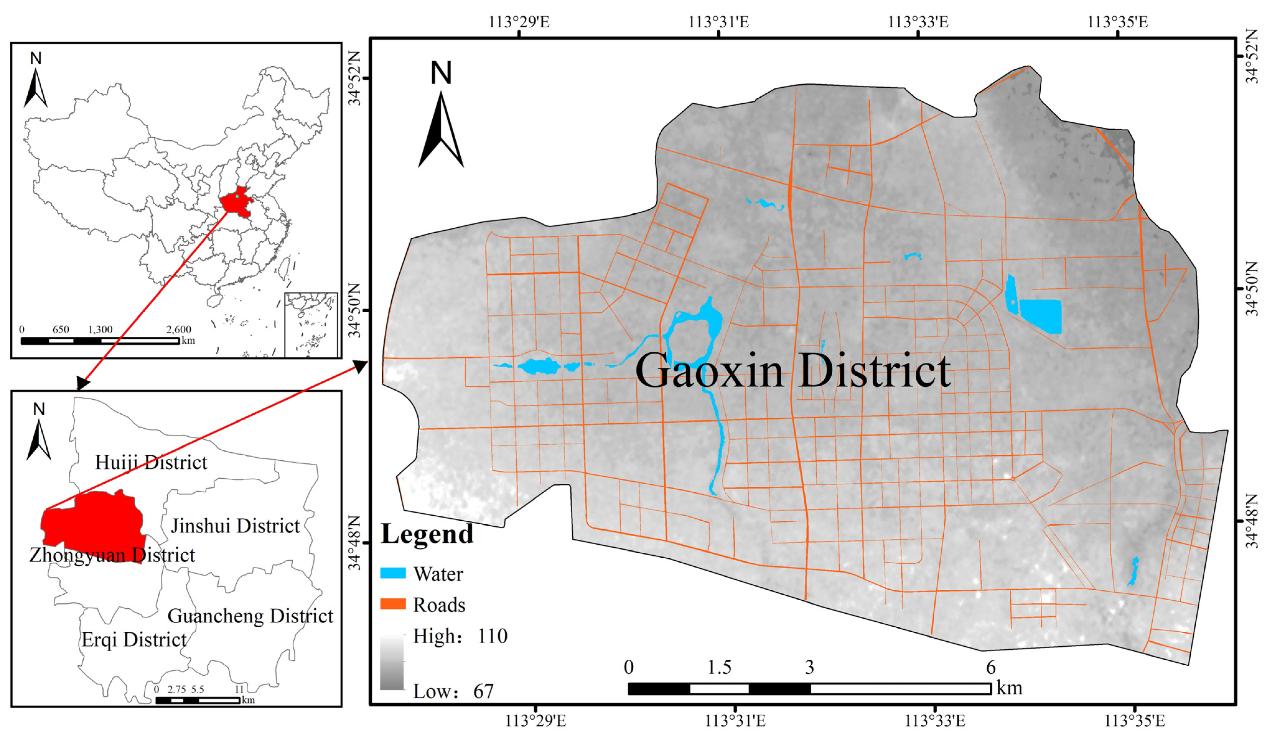
The Zhengzhou National High-Tech Industrial Development Zone is located in the northwestern part of Zhengzhou City, with a catchment area of 99 km2. Urban precipitation is mainly discharged through river networks, nullahs, and culverts across the city. The terrain is flat, with an average slope of 0.29% and an altitude range of 67 to 110 m. As shown in Figure 1, the region is predominated by temperate continental monsoon climate with four distinct seasons and an average annual rainfall of 542.1 mm. Precipitation is unevenly distributed throughout the seasons and mainly concentrated in summer, resulting in severe spring droughts and summer floods. The land cover may be classified into four categories: buildings, roads, vegetation, and bare ground, with an impervious ratio of about 62.08%.
The data requirements for SWMM model setup include rainfall data, slope and elevation, land use data, stormwater pipe system, and discharge data. The rainfall data include 1-h interval rainfall data from May to August 2018, available from meteorological stations in the Zhengzhou High-tech Zone. For the validation of the model, discharge flows with a time step of 10 min were collected. The land use data were extracted from Landsat 8 remote sensing images. Domain elevation is described by the DEM (12.5 m × 12.5 m) collected by ALOS satellite. The data were obtained from the ASF website (https://search.asf.alaska.edu), accessed on 6 April 2021. The slope was extracted using the Hydrological Analysis module to process the data, analyze the “slope” function to obtain a slope map, and then superimpose it on the sub-catchments to obtain the average slope.
2.2. Methods
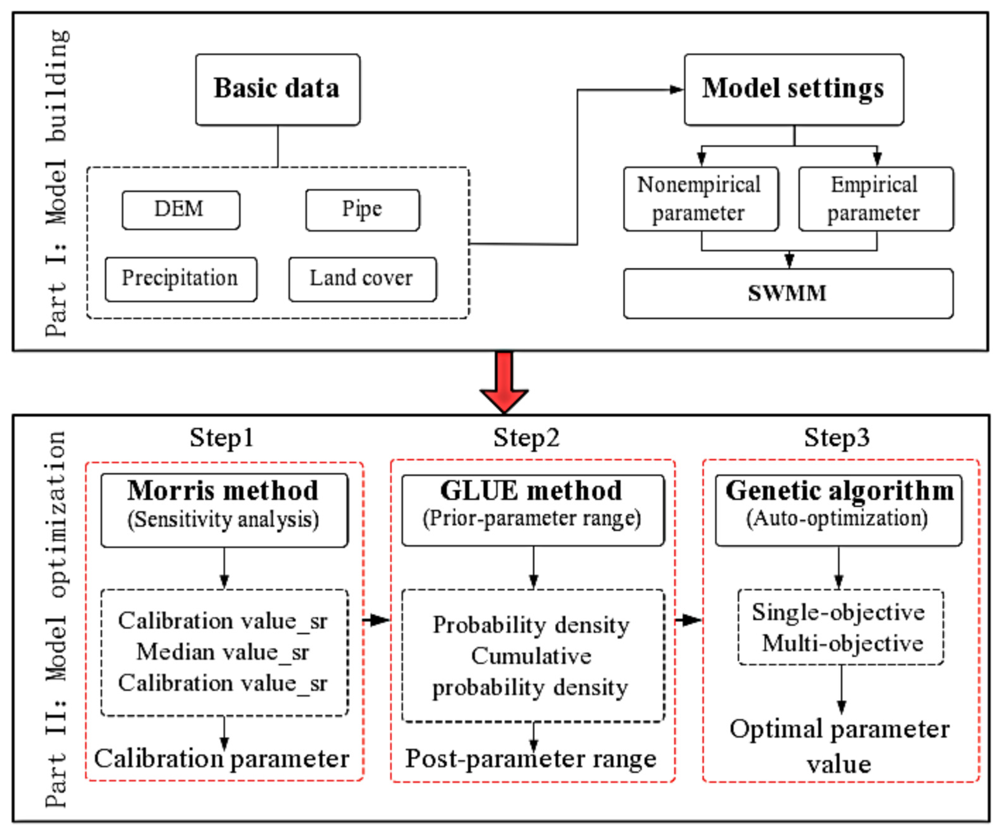
Figure 2 illustrates the flowchart of the proposed research procedure in the study, including SWMM modeling and model parameter optimization. Model parameter optimization consists of three steps: (1) sensitivity analysis to select the optimization parameters by using Morris screening method, (2) uncertainty analysis to narrow the parameter optimization interval using the GLUE method, and (3) finally using the Genetic Algorithm to further optimize the model parameters by considering objective constraints.
2.2.1. SWMM Model
The USEPA (United States Environmental Protection Agency) Storm Water Management Model (SWMM) is an urban hydrological model developed in 1971 by the United States Environmental Protection Agency to handle the expanding urban drainage problem. It is a hydrological hydrodynamics-based urban storm water model primarily used to simulate both water quantity and quality during a single rainfall event or continuous rainfall process in cities [29,30,31,32]. The model parameters of SWMM can be divided into two categories: nonempirical parameters and empirical parameters. Nonempirical parameters such as characteristic width, slope, and percent imperviousness area can be measured from field data, while empirical parameters such as permeable area, roughness coefficient, impervious area, roughness coefficient, and Horton infiltration parameter should be considered with the actual conditions of the study area and relevant literature to determine the ranges of parameter values [33,34,35,36]. It is noted that a broader range of parameter variation provides more vital information about the effect of the parameters on the model output [17]. Table 1 summarizes the main parameters of the model under study.
Different rainfall intensities lead to different results from parameter sensitivity analysis, causing specific differences in model output performance. As shown in Table 2, rainfall events with different rainfall intensities are selected and tested in this study. Among them, events 0819 and 0515 are used to complete the rainfall input for the model calibration period, while 0801 and 0730 are used as the rainfall input for the model validation period.
2.2.2. Morris Screening Method
The Morris screening method [37,38] entails choosing one of the variables, xi, from the examined parameters, holding the remaining parameter values fixed, and altering the variable xi at random within the variable’s value range. The model is then run to acquire the outcomes of various xi corresponding to the goal function y(x) = y(x1,x2,x3,…,xn). Finally, the influence value, ei, is employed to calculate the effect of input parameter changes on model output:
where y* is the output value after the parameter change, y is the output value before the parameter change, and ∆i is the value of the magnitude of the parameter i change.
The modified Morris screening method employs independent variables to vary in fixed steps, and the final sensitivity discriminant is taken as the average of multiple Morris coefficients, calculated as follows:
where S is the parameter sensitivity index; Yi is the output value of the ith run of the model; Yi + 1 is the output value of the i + 1th run of the model; Y0 is the initial value of the calculated result after parameter calibration; Pi is the percentage change in the ith model operation relative to the parameter value after calibration; Pi + 1 is the percentage change in the i + 1th model operation relative to the parameter value after calibration; n is the number of model runs.
When the value of |S| is less than 0.05, the parameter is insensitive. The parameter is moderately sensitive if the value of |S| ranges between 0.05 and 0.2. If the value of |S| ranges between 0.2 and 1.0, the parameter is considered sensitive. A value of |S| greater than 1.0 indicates that the parameter is very sensitive [39]. However, the modified Morris screening method usually selects the parameter’s initial value. It then varies a parameter by a fixed step and perturbation range [16], so the sensitivity analysis results may be affected by the initial value of the parameter and the perturbation range. If only a single sampling technique is used for the Morris screening method, the ideal parameter identification and ranking often cannot be obtained, which may cause misclassification. Therefore, this study sets three sampling methods with 2% step changes. The initial calibration is used as the initial parameter value, using a perturbation in the same range on both sides of the initial value. The initial value selects the median value of the parameter range, and perturbation is performed within the same range on both sides of the initial value (e.g., ±10%). The initial calibration is used as the initial parameter value, and the initial value is perturbed in different ranges on both sides (e.g., +10% and −30%). Each parameter has the same number of perturbations in the three sampling methods (Calibration value_sr, Median value_sr, and Calibration value_dr).
2.2.3. GLUE Method
GLUE is one of the widely used methods to evaluate model uncertainty based on Bayesian theory [40,41]. Generally, the Kolmogorov–Smirnov test is performed by parameter prior-distribution and post-distribution. The distance, D, between the overall distribution of the sample is calculated, then the model parameter sensitivity sort can be achieved [42,43]. When the two distributions are close to each other, the distance naturally decreases, and the sensitivity of the corresponding parameter is small, and vice versa. The analysis process generally consists of the following steps:
- Step 1—Selecting the likelihood function for the model simulation calculation.
- Step 2—Selecting the initial range of the model parameters and the prior distribution of parameters. The random combination of parameters is then obtained by Latin hypercube sampling.
- Step 3—Simulating the likelihood values of each combination by running the model to obtain the posterior distribution of the parameters.
Because the prior distribution of the parameters is hard to determine, uniform distribution is usually assumed. In addition, this approach does not filter sensitive parameters from non-sensitive parameters. A significant interaction effect between the input parameters leads to a change in the model output results, whereas the D value is zero at this time [44]. In this study, the GLUE method is mainly used to narrow the range of parameters further. It is combined with sensitivity analysis to reduce the solution space of parameters in the next step of model optimization. The Nash–Sutcliffe efficiency index is selected as the likelihood measure for constructing the posterior distribution of the parameters [45]. In the hydraulic modeling of urban drainage systems, the Nash–Sutcliffe efficiency index is frequently selected as a threshold value of 0.7 [46].
2.2.4. Coupling Based on Genetic Algorithm
The integration of Morris and GLUE involves several steps: (1) the parameters to be calibrated are screened by multiple Morris syntheses, (2) the GLUE uncertainty analysis is used to narrow down the range of essential parameters, and (3) the set of parameters obtained by combining the two is used for model parameter optimization. Currently, the Genetic Algorithm [47,48] has been widely used. A standard Genetic Algorithm is used to compare and analyze the effectiveness of the coupled methods, considering single and multi-objectives to construct the fitness function. Therefore, two objective formulas are considered, minimizing the sum of the squared difference objective at each moment and minimizing the peak flow error objective. These formulas have motivated a series of numerical experiments involving: (1) a single-objective calibration that considers only the sum of squared difference at each moment (Y1); (2) a multi-objective calibration that considers both objectives (Y1 and Y2).
where Y1 and Y2 are the two target minima; Qo(i) is the observed value at the moment i; Qs(i) is the simulated value at the moment i; Qps is the peak value of the flow simulation process; Qpo is the peak value of the flow observation process.
3. Results
3.1. Parameter Sensitivity Analysis
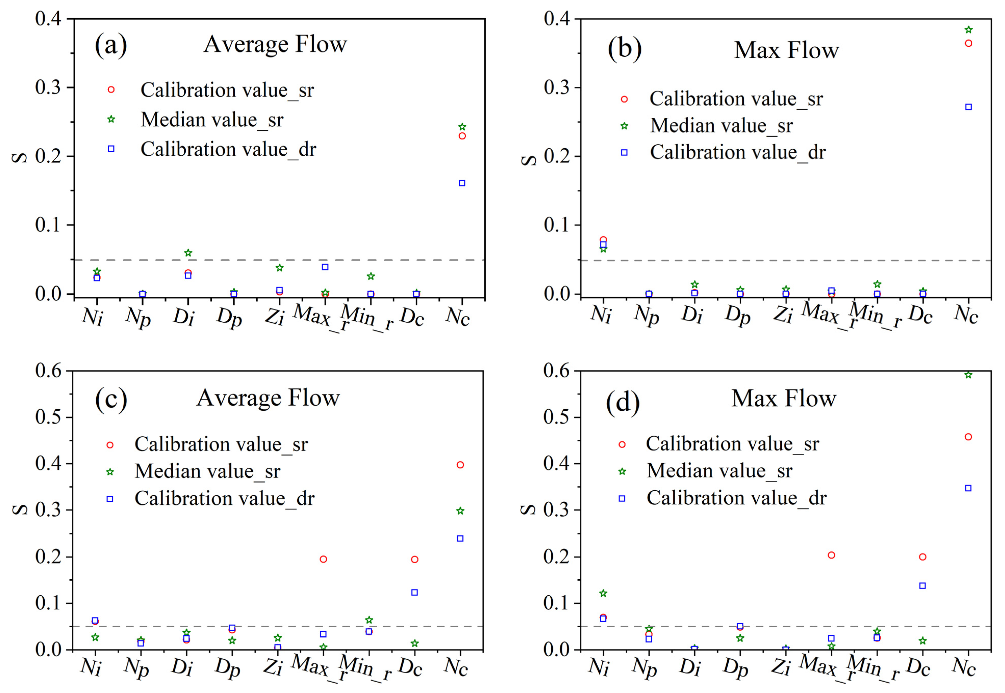
Figure 3 shows the results of the sensitivity analysis of the Morris screening method for different sampling methods and various rainfall intensities. The sensitivity analysis results show that different objective functions yield different sensitivity parameters for the same rainfall event. For changes in rainfall events, the number of sensitive parameters also differs. As shown in Figure 3a, the Nc parameter has a substantially higher sensitivity index than other parameters, significantly influencing the model simulation outcomes. In the Median value_sr technique, the Di parameter is considered sensitive only when the index value surpasses 0.05. Although the rest of the parameters do not meet the sensitivity discriminant, the sensitivity values fluctuate dramatically between the different sampling methods (e.g., Zi, Max_r, and Min_r). When looking at the flood peak simulation (Figure 3b), the sensitivity index value of the Ni parameter changes from 0.02 to 0.07, and the parameter sensitivity changes from insensitive to sensitive. The contribution of the parameter Ni to the model is significantly higher than the Di parameter, which is below the threshold value. As the intensity of the rainfall increases, the differences in parameter sensitivity between the approaches become greater. As in Figure 3c, the parameter Dc sensitivity index is below the threshold of 0.05, but the results in the other methods reach 0.12 and 0.19, respectively. Meanwhile, the Max_r parameter only meets the discriminatory criteria for sensitive parameters in the Calibration value_sr approach and is considered insensitive in the other two techniques. Although the differences in the sensitivity S values of different methods are minor for other parameters, there are still changes in the identification of sensitive and insensitive parameters (e.g., Ni, Dp, and Min_r). Thus, for the SWMM model selection optimization parameters, it is recommended to use the Morris screening method of multiple perturbation ways.
Table 3 lists the group of sensitive parameters and synthetically selected parameters for each mode. The sensitive parameters identified by various sampling methods differ, and the number of sensitive parameters identified increases with rainfall intensity. In particular, Calibration value_sr exposes sensitivity to only two parameters (Ni and Nc) for rainfall event 0819 but identifies four sensitive parameters (Ni, Nc, Dc, and Max_r) for rainfall event 0515. Ordinarily, parameters are considered to be insensitive below a threshold of 0.05. Nevertheless, this insensitivity is relative to the more sensitive parameters. Insensitivity parameters are considered to have little effect on the model. Their role in parameter optimization is often neglected; inconsistent results are easily obtained when only a single perturbation approach is used. This study comprehensively selects the calibration parameters through the sensitivity analysis results of three perturbation methods. The sensitivity index, S, of the parameters will remain consistent below the threshold value, but the index S fluctuates widely between the different ways, even close to the threshold value. For instance, the parameters Zi, Max r, Min r, and Dp in the rainfall events of 0819 and 0515 are compatible with the phenomenon mentioned above. It is similar to using a ranking approach to select the optimization parameters. In addition, two parameters are consistently identified as sensitive in this study area (Ni and Nc) despite the differences in sampling methods and rainfall events.
3.2. Uncertainty Analysis of Parameter Value Range
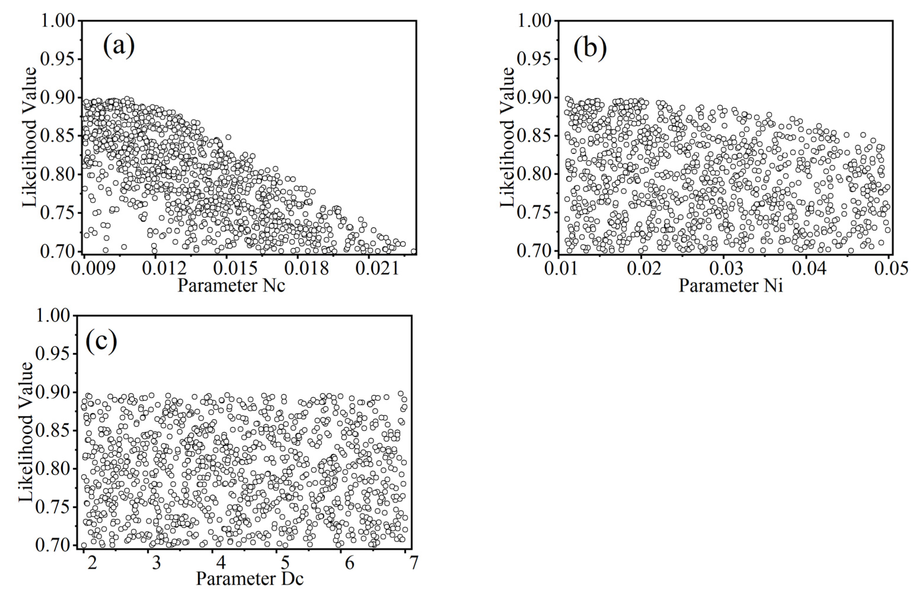
Figure 4 shows the posterior distribution of parameters and the correlation information between the behavioral parameter values and the NSE. The Latin hypercube sampling (LSH) method was employed in the study to generate a random combination of 2000 sample groups. The objective function values were acquired after numerous parameter replacements and model runs. The parameter Nc, followed by the parameter Ni, was discovered to be the most crucial calibration parameter. The parameter Dc has almost no shape peaks compared to the other two parameters.
Table 4 reports the parameters’ mean, standard deviation, and correlation matrix of the posterior distribution. There is a weak correlation between the parameters. The parameter NC has a negative correlation with the remaining two parameters, while there is a positive correlation between the parameter Ni and the parameter Dc.
Figure 5 shows the probability density plot and cumulative distribution plot of the behavioral parameter values and the Nash efficiency coefficients. The viable parameter groups that satisfy the probability objective function (NSE > 0.7) are then tallied. The remaining seven parameters have similar uniform distribution phenomena, except for Nc and Ni. Therefore, only Nc, Ni, and Dc are listed for analysis in this study. In a probability density plot, the shape of the parameter distribution indicates the frequency of the estimated uncertainty, and the lower frequency of a parameter at a certain value indicates that the parameter has more uncertainty. Nc and Ni show a trapezoidal distribution. The remaining parameters are more uniformly distributed in their respective ranges, with an extensive range of uncertainties, which often exist in the actual model simulation process with heterogeneous parameters and homogeneity. Because the more concentrated intervals cannot be obtained from the posterior distribution, the range of parameter values remains uniformly distributed, increasing parameter optimization’s difficulty. The posterior distribution differs from the prior distribution more noticeably when the parameter Nc is studied, and it is thought to be an extremely sensitive parameter. When the parameter is chosen from the interval (0.009, 0.018), the cumulative probability density of NSE > 0.7 approaches 0.93. A more intensive range of parameter values is obtained, which can be narrowed down from (0.009, 0.024) to (0.009, 0.018). The posterior distribution differs from the prior distribution when the parameter Nc is studied, and it is considered to be a weakly sensitive parameter. When the parameter is taken from the interval (0.011, 0.042), the cumulative probability density of NSE > 0.7 reaches 0.91. Likewise, a more intensive range of parameter values is obtained, which can be narrowed down from (0.011, 0.05) to (0.011, 0.042). Nonetheless, the parameter Dc is approximately uniformly distributed over their range, and a concentration range of values cannot be obtained. This phenomenon exists for seven of the nine parameters selected for the model, further indicating the instability of solutions obtained when performing SWMM model parameter optimization.
3.3. Parameter Calibration
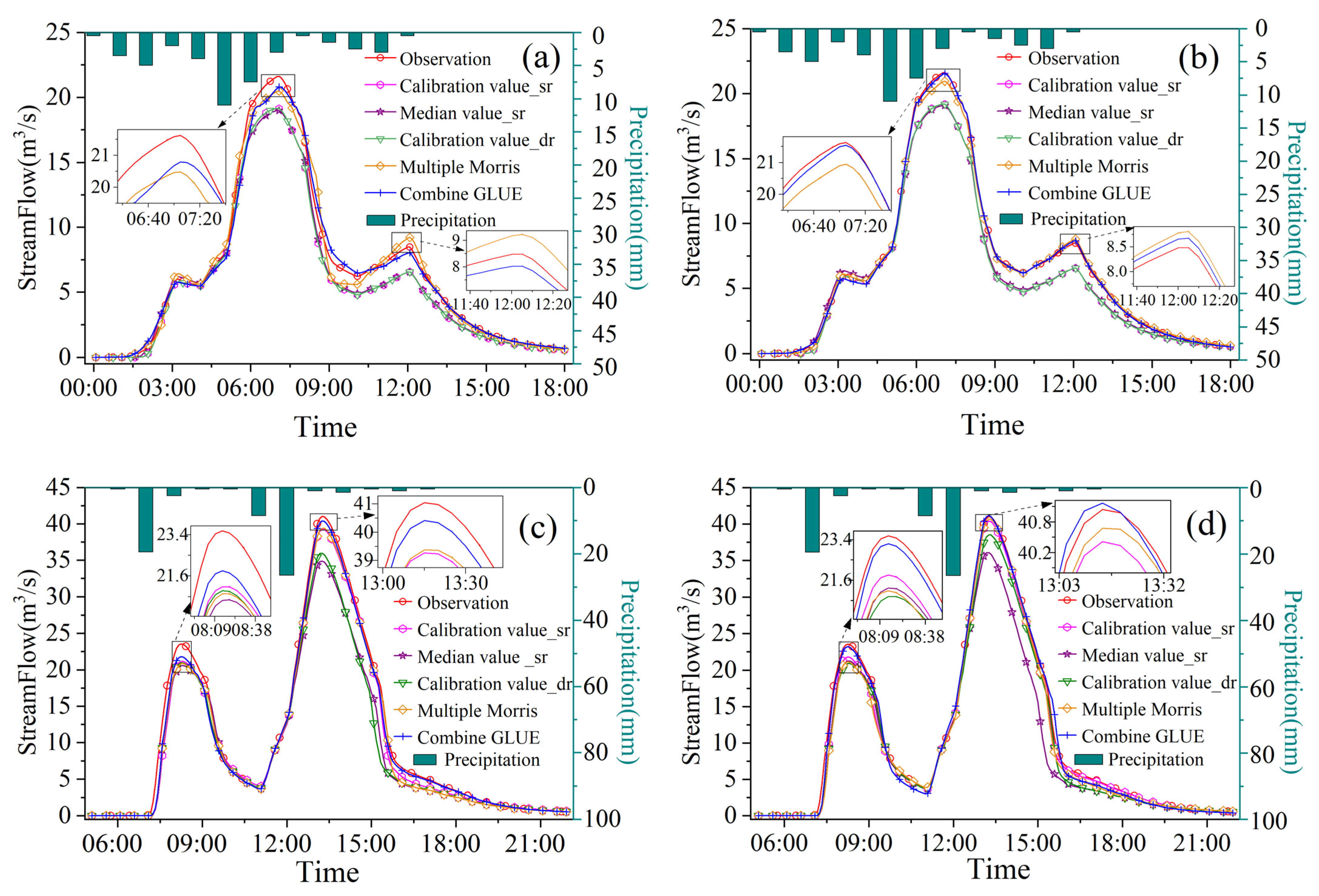
Figure 6 shows the improvement of the model simulation accuracy with parameter optimization interval reduction and also compares the effect of the Genetic Algorithm on the flood flow before and after adding the objective function constraint. This study used the Genetic Algorithm to examine the advantages of the parameter set determined by integrating Morris and GLUE methods during model parameter optimization. In the sensitivity analysis, comparative optimization experiments were also carried out for the combination of parameters to be calibrated under each perturbation approach. For the optimization of SWMM model parameters, the combined three perturbation ways sensitivity analysis screening parameters always dominate a certain position, even in the case of a single-objective constraint algorithm. By comparing (a,b) in Figure 6, the increase in the target constraint significantly improves the accuracy of the model flow simulation, with a maximum reduction in flood error of 5.1% and 3.2% for both multiple Morris and combined GLUE, respectively. For the combined GLUE method, the parameter set after narrowing the parameter value range always reduces the peak flow error during calibration. In (d) of Figure 6, the SWMM model flow simulation, combined with the GLUE method to narrow the range of the parameters, reduced the flood peak errors by 1.2% and 9% in the two flood peaks, respectively. There are still some inevitable discrepancies between the optimization of model parameters and observed flows for different rainfall events, which may be caused by the pursuit of more accurate peak flow, as in Figure 6c. In general, these deviations are within a relatively small range. There are no significant differences between the parameters determined by Morris combined with the GLUE method and the observed flow results during the optimization of model parameters.
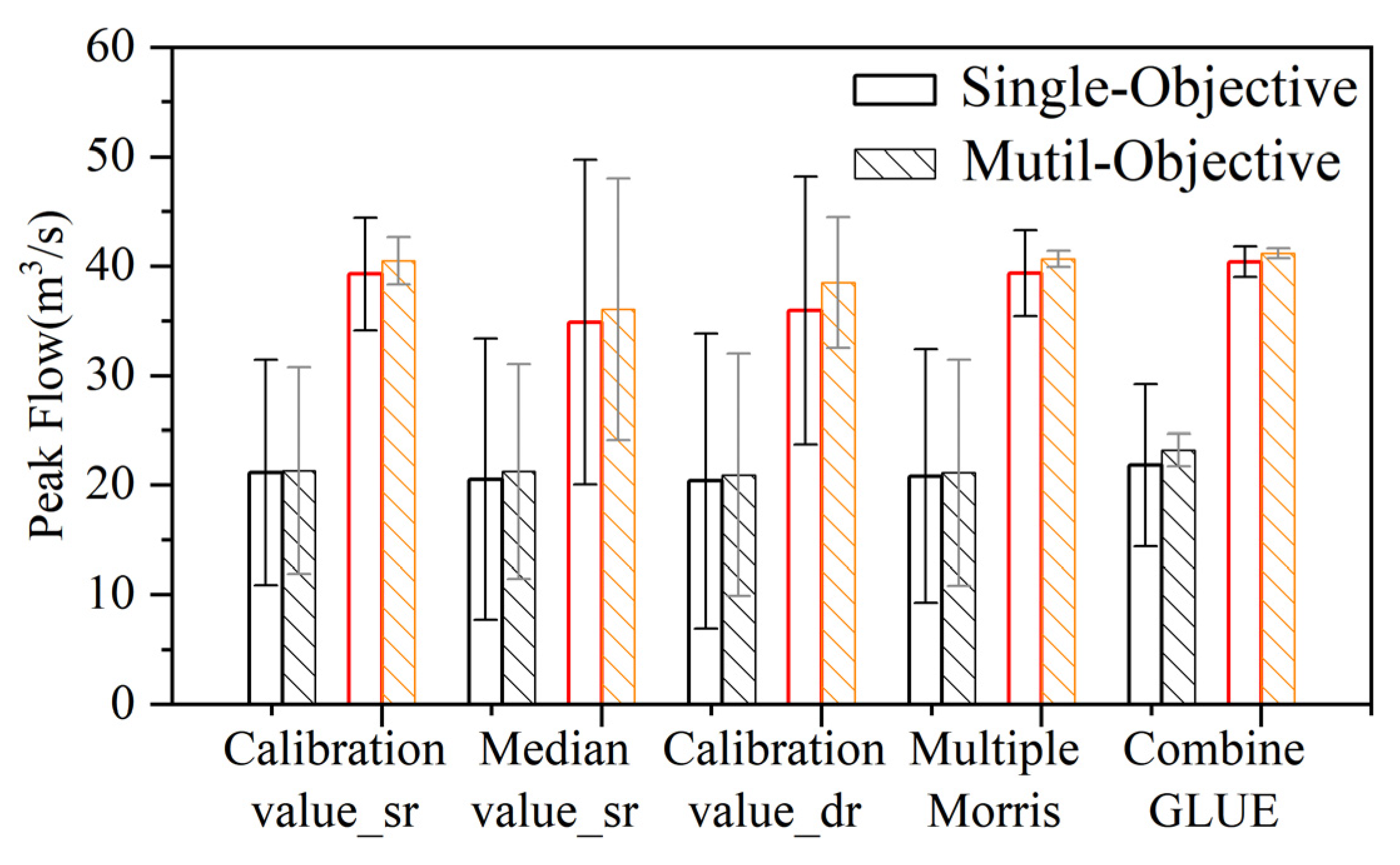
Figure 7 further visualizes the difference in peak flows under the two rainfall events. It is noticeable that the number of objective constraints and the narrowing of the parameter value range have a significant effect on the calibration of the model parameters. For the single-objective constraint algorithm in the 0515 rainfall event, the simulated peak flood errors of the models with different optimized parameter sets reached a high of 13.5% and a low of 7.4%. In comparison, the peak error decreases from a maximum of 11.1% to 1.5% with the addition of the objective function constraint. Compared with the single-objective optimization function, the Genetic Algorithm with the addition of flooding error reduces the peak error overall to a certain extent. At the same time, the enhancement of the model flow simulation accuracy by narrowing the parameter optimization interval can also be observed after combining the GLUE method compared to the synthesized Morris-screened parameters, reducing the peak error by 4.2% and 9% for the single-objective and multi-objective cases, respectively. Meanwhile, for the single-objective constraint algorithm in rainfall event 0819, the simulated peak flood errors of the models with different optimized parameter sets reached a high of 12.2% and a low of 3.8%. In comparison, the peak error decreases from a maximum of 11.8% to 0.4% with the addition of the objective function constraint. Therefore, attention should be paid to the possible impact of a more accurate parameter optimization space on algorithm optimization search during the study.
Table 5 shows the optimized parameter values of the model parameters for the two rainfall events with the original parameter values. The model’s simulation results optimized by the Genetic Algorithm are more satisfactory than the calibration values of the parameters obtained by the manual trial-and-error method in the early stages. Certain parameters’ values are taken with a greater degree of uncertainty, perhaps due to the manual trial-and-error technique being changed based on the sensitivity of the parameters, which cannot predict the nonlinear connection between the parameters and the output variables throughout the whole extraction space and is very subjective. In contrast, the Genetic Algorithm can use its powerful implicit parallelism and global optimization-seeking ability to find the best value of the parameters in the extraction space. Thus, the optimization results of model parameters differ for different rainfall, and the model parameters should be calibrated for different event types.
3.4. Validation Result
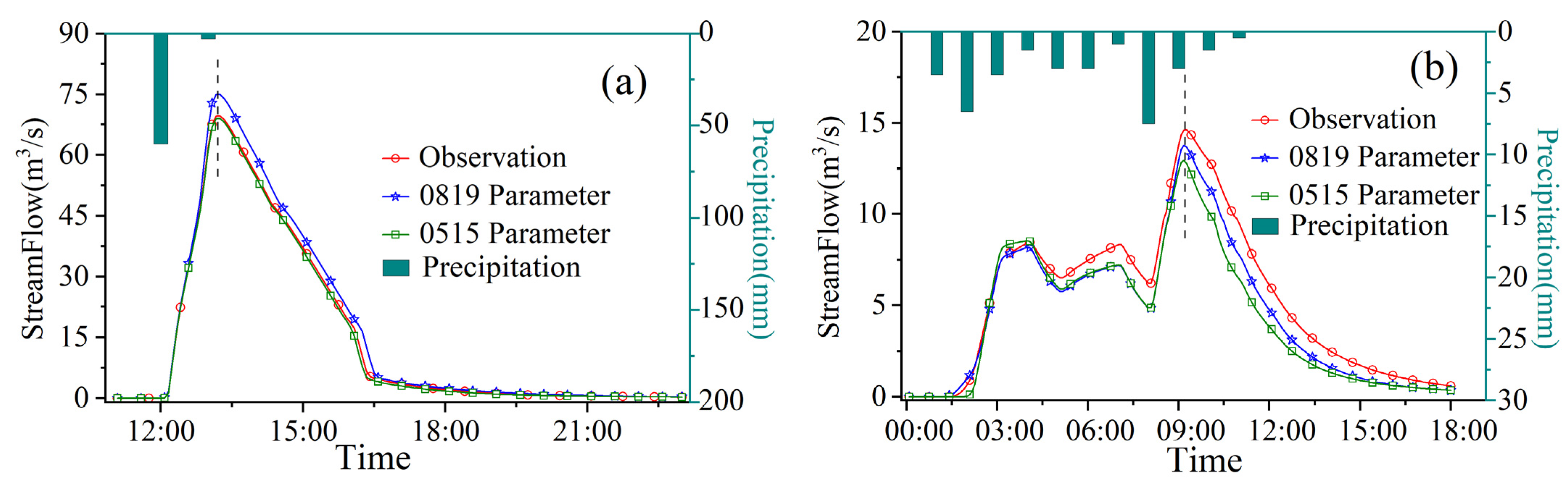
The two remaining rainfall events in the study (i.e., 0801 and 0730) were used for validation to test the applicability of the final parameter set obtained from previous experiments from the integrated Morris and GLUE method. Figure 8 shows the simulated flows received using the optimized parameter pickups for rainfall events 0819 and 0515, respectively, and the observed flows for that period. During the validation period, the parameter set determined by the integrated method can capture the same process of experimental flow under different rainfall events through a Genetic Algorithm with added objective constraints. Note that the optimized values of the parameters of different rainfall event models have some differences in adaptability. As shown in Figure 8a, the relative errors of the two sets of parameters taken at the flood position reach 0.9% and 7.7%. However, there are still some unavoidable discrepancies between optimal parameter value model simulations and observed flows, which overestimate or underestimate the flow values to some extent. For Figure 8b, using the 0515 parameter group does not have obvious advantages compared with the 0801 rainfall event simulation. The simulated process flow error is as high as 20% after the peak, possibly due to the difference in precipitation. In general, it is expected to see such differences as rainfall intensity and patterns change. The model’s optimal parameter values may need to adapt for different rainfall events.
4. Discussion
Parameter uncertainty is a common problem in complex model applications. In order to improve the simulation performance of SWMM, this study used a Genetic Algorithm optimization process combining Morris and GLUE methods. On one hand, the results from the Morris screening sensitivity analysis by combining the three sample techniques reduce the uncertainty associated with the selection of optimization parameters. For sensitivity analysis, differences in the results of parameter sensitivity analysis between different sampling methods and objective functions can be found, and even sudden changes in parameter sensitivity may occur. Some researchers concluded that the main relevant factors affecting the SWMM model results were the Manning coefficients for impervious zone and pipes, whereas Horton’s infiltration coefficient was recognized as a particularly sensitive parameter [49,50]. The optimized parameters selected in this study by combining the results of the three sensitivity analyses coincide with these conclusions. For rainfall event 0819, only the sensitive parameter set is considered for optimization, ignoring the parameters related to Horton’s infiltration coefficient that significantly impact the model. Although several of the parameters are classified as insensitive parameters (e.g., Zi, Max_r, Min_r), leaving them out will produce worse model simulation results. Even though it will increase part of the parameter optimization workload (e.g., Zi), the overall benefits still outweigh the disadvantages. For this reason, the Morris screening method only considers the screening results under a single perturbation approach, increasing the uncertainty in parameter selection [51,52,53,54]. In addition, wider parameter optimization intervals tend to expand the scope of algorithm search during optimization, leading to more significant model simulation errors and reducing algorithm search efficiency. From the parameter optimization results, the peak error reduction of 9% achieved by combining the GLUE method to narrow the parameter range improves the algorithm’s accuracy for model parameter optimization. The parameter optimization interval may be one of the influencing factors for the poor simulation accuracy of the model after optimization using the algorithm [55]. Therefore, it is necessary to optimize the model parameters using a combination of sensitivity analysis and uncertainty analysis to determine the parameters to be optimized. In this study, after determining the parameters involved in optimization, the Genetic Algorithm with a single-objective function constraint and the multi-objective constraint case were used for comparative analysis, respectively. During the optimization of model parameters for different rainfall events, the overall trend of model simulation error decreases when the objective function constraint is added in constructing the fitness function. Generally, the Genetic Algorithm with multi-objective constraints has better performance [56].
There are still some limitations in this study. Only two of the nine parameters involved in the model optimization obtained a reduced range of values using the GLUE method in combination with the sensitivity analysis process. Nevertheless, for a complex hydrological model, it is common to involve more parameters in model optimization. Often more than one parameter in different models and study areas can be used to obtain more accurate parameter intervals by uncertainty analysis [57,58,59]. Considering a suitable range of uncertainty parameter values after sensitivity analysis for model parameter optimization will further improve the model simulation accuracy. Adding the objective constraint function in constructing the fitness function may not be perfect compared with other multi-objective Genetic Algorithms. Despite the limitations in this study, the optimization process of the Genetic Algorithm based on the integrated Morris and GLUE method still improves SWMM’s simulation accuracy. The uncertainty involving the selection of optimization parameters is reduced, and the algorithm’s optimization-seeking interval is narrowed. In particular, the N-conduit is reduced from (0.009, 0.024) to (0.009, 0018), and the N-imperv is reduced from (0.011, 0.05) to (0.011, 0.042). This study’s threshold value is 0.7 for NSE, widely selected in urban hydraulic modeling. Selecting different thresholds results in distinct sets of behavioral parameters. As the threshold value selected for the likelihood objective function increases, the range of practical parameter sets taken is smaller. Although the reduction in the range of values is insignificant, it reduces the average 3.2% peak error of the model simulation during the optimization period (Table 6). Furthermore, after adding the objective function constraint, the Genetic Algorithm further reduces the error of the model flow simulation process.
5. Conclusions
This study proposed a SWMM model parameter optimization procedure including parameters sensitivity analysis, uncertainty analysis, and Genetic Algorithms to enhance flow simulation results. By combining three sampling methods, the parameters to be optimized are selected through the Morris screening method. The ideal range of values of the parameters were analyzed with the GLUE method. In addition, single-objective and multi-objective constrained Genetic Algorithms for constructing the fitness function are used to optimize the model parameters, respectively. The main conclusions are as follows:
- (1)
- The parameter sensitivity analysis results varied with the different objective functions utilized. The sensitive factors are also observed to change with the rainfall intensity. These indicate that it is essential to consider multiple operating conditions in the parameter sensitivity analysis. In addition, the perturbation analysis of multiple modalities shows that the sensitivity of the parameters is highly susceptible to sudden changes among different modalities, and the results of the screening method for a single perturbation modality possess considerable uncertainty.
- (2)
- Although the GLUE method only reduced the range of the values for two parameters in the research, the peak error was reduced by up to 9%. For the optimization of complex model parameters, using sensitivity and uncertainty analysis in combination with each other, satisfactory model simulation results can be achieved.
- (3)
- When the Genetic Algorithm was used to optimize parameter sets with different combinations, the model parameter optimization process varied with the increase in the number of constraints on the fitness function. Compared with constructing the fitness function using a single-objective constraint, the Genetic Algorithm for multi-objective constraints shows a decreasing trend in the overall peak error of the model simulations.
Author Contributions
Conceptualization, H.Y. and B.Z.; methodology, Z.W. and B.Z.; writing—original draft preparation, B.Z.; writing—review and editing, Z.W., Q.L., H.X., M.G. and B.Z.; supervision, H.Y.; project administration, H.Y.; funding acquisition, H.Y. All authors have read and agreed to the published version of the manuscript.
Funding
This research was supported by the National Key R&D Program of China (grant number 2022YFC3004402), the Henan provincial key research and development program (221111321100), and the National Natural Science Foundation of China (No: 51739009).
Data Availability Statement
Not applicable.
Acknowledgments
We are grateful to the editors and anonymous reviewers for their thoughtful comments.
Conflicts of Interest
The authors declare no conflict of interest.
References
- Veal, A.J. Climate change 2021: The physical science basis, 6th report. World Leis. J. 2021, 63, 443–444. [Google Scholar] [CrossRef]
- Zhang, L.; Jin, X.; He, C.; Zhang, B.; Zhang, X.; Li, J.; Zhao, C.; Tian, J.; DeMarchi, C. Comparison of SWAT and DLBRM for Hydrological Modeling of a Mountainous Watershed in Arid Northwest China. J. Hydrol. Eng. 2016, 21, 1313. [Google Scholar] [CrossRef]
- Iffland, R.; Förster, K.; Westerholt, D.; Pesci, M.; Lösken, G. Robust Vegetation Parameterization for Green Roofs in the EPA Stormwater Management Model (SWMM). Hydrology 2021, 8, 12. [Google Scholar] [CrossRef]
- Ballinas-González, H.; Alcocer-Yamanaka, V.; Canto-Rios, J.; Simuta-Champo, R. Sensitivity Analysis of the Rainfall–Runoff Modeling Parameters in Data-Scarce Urban Catchment. Hydrology 2020, 7, 73. [Google Scholar] [CrossRef]
- Szeląg, B.; Kiczko, A.; Łagód, G.; De Paola, F. Relationship Between Rainfall Duration and Sewer System Performance Measures Within the Context of Uncertainty. Water Resour. Manag. 2021, 35, 5073–5087. [Google Scholar] [CrossRef]
- Hussain, S.N.; Zwain, H.M.; Nile, B.K. Modeling the effects of land-use and climate change on the performance of stormwater sewer system using SWMM simulation: Case study. J. Water Clim. Chang. 2021, 13, 125–138. [Google Scholar] [CrossRef]
- Cukier, R.I.; Levine, H.B.; Shuler, K.E. Nonlinear sensitivity analysis of multiparameter model systems. J. Phys. Chem. 1977, 81, 2365–2366. [Google Scholar] [CrossRef]
- Lei, J.; Schilling, W. Parameter Uncertainty Propagation Analysis for Urban Rainfall Runoff Modelling. Water Sci. Technol. 1994, 29, 145–154. [Google Scholar] [CrossRef]
- Knighton, J.; White, E.; Lennon, E.; Rajan, R. Development of probability distributions for urban hydrologic model parameters and a Monte Carlo analysis of model sensitivity. Hydrol. Process. 2013, 28, 5131–5139. [Google Scholar] [CrossRef]
- Dong, Q.; Lu, F. Performance Assessment of Hydrological Models Considering Acceptable Forecast Error Threshold. Water 2015, 7, 6173–6189. [Google Scholar] [CrossRef]
- Liu, Z.J.; Li, L.H. An Evaluation Method of Water Quality Based on Improved PSO-BP Network. Adv. Mater. Res. 2013, 846, 1243–1246. [Google Scholar] [CrossRef]
- Zhou, L.; Liu, P.; Gui, Z.; Zhang, X.; Liu, W.; Cheng, L.; Xia, J. Diagnosing structural deficiencies of a hydrological model by time-varying parameters. J. Hydrol. 2022, 605, 127305. [Google Scholar] [CrossRef]
- Confalonieri, R.; Bellocchi, G.; Tarantola, S.; Acutis, M.; Donatelli, M.; Genovese, G. Sensitivity analysis of the rice model WARM in Europe: Exploring the effects of different locations, climates and methods of analysis on model sensitivity to crop parameters. Environ. Model. Softw. 2010, 25, 479–488. [Google Scholar] [CrossRef]
- van der Sterren, M.; Rahman, A.; Ryan, G. Modeling of a lot scale rainwater tank system in XP-SWMM: A case study in Western Sydney, Australia. J. Environ. Manag. 2014, 141, 177–189. [Google Scholar] [CrossRef]
- Sreedevi, S.; Eldho, T.I. A two-stage sensitivity analysis for parameter identification and calibration of a physically-based distributed model in a river basin. Hydrol. Sci. J. 2019, 64, 701–719. [Google Scholar] [CrossRef]
- Lin, J.; Zou, X.; Huang, F. Quantitative analysis of the factors influencing the dispersion of thermal pollution caused by coastal power plants. Water Res. 2020, 188, 116558. [Google Scholar] [CrossRef]
- Freni, G.; Mannina, G.; Viviani, G. Uncertainty in urban stormwater quality modelling: The influence of likelihood measure formulation in the GLUE methodology. Sci. Total Environ. 2009, 408, 138–145. [Google Scholar] [CrossRef]
- Zhang, H.; Chang, J.; Zhang, L.; Wang, Y.; Ming, B. Calibration and uncertainty analysis of a hydrological model based on cuckoo search and the M-GLUE method. Arch. Meteorol. Geophys. Bioclimatol. Ser. B 2018, 137, 165–176. [Google Scholar] [CrossRef]
- Liang, Y.; Cai, Y.; Sun, L.; Wang, X.; Li, C.; Liu, Q. Sensitivity and uncertainty analysis for streamflow prediction based on multiple optimization algorithms in Yalong River Basin of southwestern China. J. Hydrol. 2021, 601, 126598. [Google Scholar] [CrossRef]
- Muronda, M.T.; Marofi, S.; Nozari, H.; Babamiri, O. Uncertainty Analysis of Reservoir Operation Based on Stochastic Optimization Approach Using the Generalized Likelihood Uncertainty Estimation Method. Water Resour. Manag. 2021, 35, 3179–3201. [Google Scholar] [CrossRef]
- Chen, X.; Yang, T.; Wang, X.; Xu, C.-Y.; Yu, Z. Uncertainty Intercomparison of Different Hydrological Models in Simulating Extreme Flows. Water Resour. Manag. 2012, 27, 1393–1409. [Google Scholar] [CrossRef]
- Moges, E.; Demissie, Y.; Larsen, L.; Yassin, F. Review: Sources of Hydrological Model Uncertainties and Advances in Their Analysis. Water 2020, 13, 28. [Google Scholar] [CrossRef]
- Xue, F.; Tian, J.; Wang, W.; Zhang, Y.; Ali, G. Parameter Calibration of SWMM Model Based on Optimization Algorithm. Comput. Mater. Contin. 2020, 65, 2189–2199. [Google Scholar] [CrossRef]
- Xu, Z.; Xiong, L.; Li, H.; Xu, J.; Cai, X.; Chen, K.; Wu, J. Runoff simulation of two typical urban green land types with the Stormwater Management Model (SWMM): Sensitivity analysis and calibration of runoff parameters. Environ. Monit. Assess. 2019, 191, 343. [Google Scholar] [CrossRef]
- Behrouz, M.S.; Zhu, Z.; Matott, L.S.; Rabideau, A.J. A new tool for automatic calibration of the Storm Water Management Model (SWMM). J. Hydrol. 2019, 581, 124436. [Google Scholar] [CrossRef]
- Li, S.; Wang, Z.; Wu, X.; Zeng, Z.; Shen, P.; Lai, C. A novel spatial optimization approach for the cost-effectiveness improvement of LID practices based on SWMM-FTC. J. Environ. Manag. 2022, 307, 114574. [Google Scholar] [CrossRef]
- Perin, R.; Trigatti, M.; Nicolini, M.; Campolo, M.; Goi, D. Automated calibration of the EPA-SWMM model for a small suburban catchment using PEST: A case study. Environ. Monit. Assess. 2020, 192, 1–17. [Google Scholar] [CrossRef]
- Eckart, K.; McPhee, Z.; Bolisetti, T. Multiobjective optimization of low impact development stormwater controls. J. Hydrol. 2018, 562, 564–576. [Google Scholar] [CrossRef]
- Gironás, J.; Roesner, L.A.; Rossman, L.A.; Davis, J. A new applications manual for the Storm Water Management Model (SWMM). Environ. Model. Softw. 2010, 25, 813–814. [Google Scholar] [CrossRef]
- Liang, J.; Hu, Z.; Liu, S.; Zhong, G.; Zhen, Y.; Makhinov, A.N.; Araruna, J.T. Residual-Oriented Optimization of Antecedent Precipitation Index and Its Impact on Flood Prediction Uncertainty. Water 2022, 14, 3222. [Google Scholar] [CrossRef]
- Annus, I.; Vassiljev, A.; Kändler, N.; Kaur, K. Automatic Calibration Module for an Urban Drainage System Model. Water 2021, 13, 1419. [Google Scholar] [CrossRef]
- Lee, J.; Kim, J.; Lee, J.M.; Jang, H.S.; Park, M.; Min, J.H.; Na, E.H. Analyzing the Impacts of Sewer Type and Spatial Distribution of LID Facilities on Urban Runoff and Non-Point Source Pollution Using the Storm Water Management Model (SWMM). Water 2022, 14, 2776. [Google Scholar] [CrossRef]
- Shi, R.; Zhao, G.; Pang, B.; Jiang, Q.; Zhen, T. Uncertainty Analysis of SWMM Model Parameters Based on GLUE Method. J. China Hydrol. 2016, 36, 1–6. [Google Scholar]
- Chang, X.; Xu, Z.; Zhao, G.; Li, H. Sensitivity analysis on SWMM model parameters based on Sobol method. J. Hydro-Electr. Engineering. 2018, 37, 59–68. [Google Scholar]
- Li, M.; Yang, X. Global Sensitivity Analysis of SWMM Parameters Based on Sobol Method. China Water Wastewater 2020, 36, 95–102. [Google Scholar]
- Rossman, L.A.; Simon, M.A. Storm Water Management Model User's Manual Version 5.2; EPA: Cincinnati, OH, USA, 2022. [Google Scholar]
- Morris, M.D. Factorial Sampling Plans for Preliminary Computational Experiments. Technometrics 1991, 33, 161–174. [Google Scholar] [CrossRef]
- Zádor, J.; Zsély, I.; Turányi, T. Local and global uncertainty analysis of complex chemical kinetic systems. Reliab. Eng. Syst. Saf. 2006, 91, 1232–1240. [Google Scholar] [CrossRef]
- Lenhart, T.; Eckhardt, K.; Fohrer, N.; Frede, H.-G. Comparison of two different approaches of sensitivity analysis. Phys. Chem. Earth Parts A/B/C 2002, 27, 645–654. [Google Scholar] [CrossRef]
- Beven, K.; Binley, A. The future of distributed models: Model calibration and uncertainty prediction. Hydrol. Process. 1992, 6, 279–298. [Google Scholar] [CrossRef]
- Mirzaei, M.; Huang, Y.F.; El-Shafie, A.; Shatirah, A. Application of the generalized likelihood uncertainty estimation (GLUE) approach for assessing uncertainty in hydrological models: A review. Stoch. Hydrol. Hydraul. 2015, 29, 1265–1273. [Google Scholar] [CrossRef] [Green Version]
- Thorndahl, S.; Beven, K.; Jensen, J.; Schaarup-Jensen, K. Event based uncertainty assessment in urban drainage modelling, applying the GLUE methodology. J. Hydrol. 2008, 357, 421–437. [Google Scholar] [CrossRef] [Green Version]
- Lee, D.; Beste, M.T.; Anderson, N.R.; Koretzky, G.A.; Hammer, D.A. Identifying Key Pathways and Components in Chemokine-Triggered T Lymphocyte Arrest Dynamics Using a Multi-Parametric Global Sensitivity Analysis. Cell. Mol. Bioeng. 2019, 12, 193–202. [Google Scholar] [CrossRef] [PubMed]
- Saltelli, A.; Ratto, M.; Andres, T.; Campolongo, F.; Cariboni, J.; Gatelli, D.; Saisana, M.; Tarantola, S. Global Sensitivity Analysis. The Primer, 1st ed.; John Wiley & Sons Ltd: West Sussex, UK, 2007; pp. 1–292. [Google Scholar]
- Dotto, C.B.; Mannina, G.; Kleidorfer, M.; Vezzaro, L.; Henrichs, M.; McCarthy, D.T.; Freni, G.; Rauch, W.; Deletic, A. Comparison of different uncertainty techniques in urban stormwater quantity and quality modelling. Water Res. 2012, 46, 2545–2558. [Google Scholar] [CrossRef]
- Zhang, W.; Li, T. The Influence of Objective Function and Acceptability Threshold on Uncertainty Assessment of an Urban Drainage Hydraulic Model with Generalized Likelihood Uncertainty Estimation Methodology. Water Resour. Manag. 2015, 29, 2059–2072. [Google Scholar] [CrossRef]
- Kang, C.; Liu, Z.; Shirinzadeh, B.; Zhou, H.; Shi, Y.; Yu, T.; Zhao, P. Parametric optimization for multi-layered filament-wound cylinder based on hybrid method of GA-PSO coupled with local sensitivity analysis. Compos. Struct. 2021, 267, 113861. [Google Scholar] [CrossRef]
- Peng, Z.; Jin, X.; Sang, W.; Zhang, X. Optimal Design of Combined Sewer Overflows Interception Facilities Based on the NSGA-III Algorithm. Water 2021, 13, 3440. [Google Scholar] [CrossRef]
- Randall, M.; Sun, F.; Zhang, Y.; Jensen, M.B. Evaluating Sponge City volume capture ratio at the catchment scale using SWMM. J. Environ. Manag. 2019, 246, 745–757. [Google Scholar] [CrossRef]
- Baek, S.-S.; Choi, D.-H.; Jung, J.-W.; Lee, H.-J.; Lee, H.; Yoon, K.-S.; Cho, K.H. Optimizing low impact development (LID) for stormwater runoff treatment in urban area, Korea: Experimental and modeling approach. Water Res. 2015, 86, 122–131. [Google Scholar] [CrossRef]
- Wu, Z.; Ma, B.; Wang, H.; Hu, C.; Lv, H.; Zhang, X. Identification of Sensitive Parameters of Urban Flood Model Based on Artificial Neural Network. Water Resour. Manag. 2021, 35, 2115–2128. [Google Scholar] [CrossRef]
- Peng, J.; Yu, L.; Cui, Y.; Yuan, X. Application of SWMM 5.1 in flood simulation of sponge airport facilities. Water Sci. Technol. 2020, 81, 1264–1272. [Google Scholar] [CrossRef]
- Wang, X.; Kang, F.; Li, J.; Wang, X. Inverse Parametric Analysis of Seismic Permanent Deformation for Earth-Rockfill Dams Using Artificial Neural Networks. Math. Probl. Eng. 2012, 2012, 383749. [Google Scholar] [CrossRef] [Green Version]
- Sang, X.; Zhou, Z.; Wang, H.; Qin, D.; Zhai, Z.; Chen, Q. Development of Soil and Water Assessment Tool Model on Human Water Use and Application in the Area of High Human Activities, Tianjin, China. J. Irrig. Drain. Eng. 2010, 136, 23–30. [Google Scholar] [CrossRef]
- Hashemi, M.; Mahjouri, N. Global Sensitivity Analysis-based Design of Low Impact Development Practices for Urban Runoff Management Under Uncertainty. Water Resour. Manag. 2022, 36, 2953–2972. [Google Scholar] [CrossRef]
- Ogidan, O.; Giacomoni, M. Multiobjective Genetic Optimization Approach to Identify Pipe Segment Replacements and Inline Storages to Reduce Sanitary Sewer Overflows. Water Resour. Manag. 2016, 30, 3707–3722. [Google Scholar] [CrossRef]
- Zhao, D.; Wang, H.; Chen, J.; Wang, H. Parameters uncertainty analysis of urban rainfall-runoff simulation. Adv. Water Sci. 2009, 20, 45–51. [Google Scholar]
- Seong, Y.; Choi, C.-K.; Jung, Y. Assessment of Uncertainty in Grid-Based Rainfall-Runoff Model Based on Formal and Informal Likelihood Measures. Water 2022, 14, 2210. [Google Scholar] [CrossRef]
- Blasone, R.-S.; Madsen, H.; Rosbjerg, D. Uncertainty assessment of integrated distributed hydrological models using GLUE with Markov chain Monte Carlo sampling. J. Hydrol. 2008, 353, 18–32. [Google Scholar] [CrossRef]
Figure 1.
Study area.

Figure 2.
Flow chart of the research methods. The first step of the red dashed box symbolizes the process of identifying the parameters to be optimized, the second step depicts the process of narrowing the range of sensitive parameter values, and the third step represents the process of automatic model parameter optimization utilizing the Genetic Algorithm.

Figure 3.
Comparing three sample techniques’ parameter sensitivity using the Morris screening method: (a) Average flow parameter sensitivity for rainfall event 0819; (b) Max flow parameter sensitivity for rainfall event 0819; (c) Average flow parameter sensitivity for rainfall event 0515; (d) Max flow parameter sensitivity for rainfall event 0515. The gray dashed line denotes the parameter sensitivity threshold.

Figure 4.
Likelihood scatters plot of parameters: (a) Relationship of parameter Nc and NSE; (b) Relationship of parameter Ni and NSE; (c) Relationship of parameter Dc and NSE. The x-axis represents the posterior distribution of the parameters.
Figure 4.
Likelihood scatters plot of parameters: (a) Relationship of parameter Nc and NSE; (b) Relationship of parameter Ni and NSE; (c) Relationship of parameter Dc and NSE. The x-axis represents the posterior distribution of the parameters.

Figure 5.
Parameter probability density plots and cumulative distribution plots: (a) Parameter Nc; (b) Parameter Ni; (c) Parameter Dc. The x-axis represents the posterior distribution of the parameters.
Figure 5.
Parameter probability density plots and cumulative distribution plots: (a) Parameter Nc; (b) Parameter Ni; (c) Parameter Dc. The x-axis represents the posterior distribution of the parameters.

Figure 6.
Model flow simulation results during the calibration period: (a) Genetic Algorithm with a single-objective for rainfall event 0819; (b) Genetic Algorithm with multi-objective for rainfall event 0819; (c) Genetic Algorithm with a single-objective for rainfall event 0515; (d) Genetic Algorithm with multi-objective for rainfall event 0515.

Figure 7.
Error charts for single-objective versus multi-objective constraint algorithms in model flow simulation. Each name corresponds to two groups of two bar charts; the group of bar charts on the left corresponds to the top peak of rainfall event 0819, and the group of bar charts on the right corresponds to the top peak of rainfall event 0515. The length of the vertical lines on the bar graphs represents the peak relative error of the model simulation.

Figure 8.
Flow simulation results using two sets of parameter during the validation period: (a) Rainfall event 0801; (b) Rainfall event 0730.
Figure 8.
Flow simulation results using two sets of parameter during the validation period: (a) Rainfall event 0801; (b) Rainfall event 0730.


Table 1.
SWMM model’s hydrological and hydraulic parameters.
| Symbol | Parameter | Description | Domain |
|---|---|---|---|
| Ni | N-imperv | Manning’s n for impervious areas | (0.011, 0.05) |
| Np | N-perv | Manning’s n for pervious areas | (0.01, 0.8) |
| Di | Destore-imperv | Depression storage for impervious areas (mm) | (0.2, 10) |
| Dp | Destore-perv | Depression storage for pervious areas (mm) | (2, 10) |
| Zi | Zero-imperv | Percent of impervious area without depression storage (%) | (5, 85) |
| Max_r | Maxrate | Maximum infiltration rate (mm.h−1) | (20, 127) |
| Min_r | Minrate | Minimum infiltration rate (mm.h−1) | (0.1, 10) |
| Dc | Decay-constant | Infiltration attenuation coefficient (h−1) | (2, 7) |
| Nc | N-conduit | Manning’s n for conduits | (0.009, 0.024) |
Table 2.
Rainfall event information.
| Event | Data | Total Rainfall (mm) | Duration (h) | Time Step (h) | Max Intensity (mm/h) |
|---|---|---|---|---|---|
| 0819 | 19 August 2018 | 41.5 | 13 | 1 | 11 |
| 0515 | 15 March 2018 | 64.5 | 12 | 1 | 26.5 |
| 0801 | 1 August 2018 | 63 | 2 | 1 | 60 |
| 0730 | 30 July 2017 | 34.5 | 12 | 1 | 7.5 |
Table 3.
Three sampling methods: SA screening sensitive parameters and a combined relatively sensitive parameter.
Table 3.
Three sampling methods: SA screening sensitive parameters and a combined relatively sensitive parameter.
| Group | 0819 | 0515 |
|---|---|---|
| Calibration value_sr | Nc, Ni | Nc, Dc, Max_r, Ni |
| Median value_sr | Nc, Ni, Di | Nc, Ni, Min_r |
| Calibration value_dr | Nc, Ni | Nc, Ni, Dc |
| Multiple Morris | Ni, Di, Nc, Zi, Max_r, Min_r | Nc, Dc, Ni, Max_r, Min_r, Dp |
Table 4.
Mean, standard deviation, coefficient of variation, and correlation matrix of the posterior distributions for the parameters.
Table 4.
Mean, standard deviation, coefficient of variation, and correlation matrix of the posterior distributions for the parameters.
| Parameter | Mean | σ | Cov | Correlation Coefficient, R | ||
|---|---|---|---|---|---|---|
| Nc | Ni | Dc | ||||
| Nc | 0.014 | 0.003 | 23% | 1 | ||
| Ni | 0.027 | 0.011 | 40% | −0.32 | 1 | |
| Dc | 4.412 | 1.444 | 33% | −0.03 | 0.01 | 1 |
Table 5.
Values set before and after parameter optimization.
| 0819 Parameter | Before Calibration | After Calibration | 0515 Parameter | Before Calibration | After Calibration |
|---|---|---|---|---|---|
| Ni | 0.013 | 0.0207 | Ni | 0.013 | 0.021 |
| Di | 2.54 | 5.1 | Dp | 7 | 5.9 |
| Zi | 0 | 47.6 | Max_r | 114.4 | 116.4 |
| Max_r | 114.4 | 27.5 | Min_r | 3.8 | 1.3 |
| Min_r | 3.8 | 0.7 | Dc | 2 | 4 |
| Nc | 0.01 | 0.011 | Nc | 0.01 | 0.012 |
Table 6.
Peak flow relative error of model simulations during the calibration and validation periods.
Table 6.
Peak flow relative error of model simulations during the calibration and validation periods.
| Rainfall Event | Method | Peak 1 Error (%) | Peak 2 Error (%) | ||
|---|---|---|---|---|---|
| Single-Objective | Multi-Objective | Single-Objective | Multi-Objective | ||
| 0819 | Calibration value_sr | 11.42 | 11.26 | 22.66 | 22.61 |
| Median value_sr | 12.17 | 11.71 | 22.76 | 22.72 | |
| Calibration value_sr | 11.51 | 11.27 | 22.55 | 22.39 | |
| Multiple Morris | 5.22 | 3.09 | 8.77 | 3.71 | |
| Combine GLUE | 3.77 | 0.36 | 5.36 | 2.18 | |
| 0515 | Calibration value_sr | 10.30 | 9.44 | 5.14 | 2.17 |
| Median value_sr | 12.83 | 9.81 | 15.72 | 12.83 | |
| Calibration value_sr | 13.46 | 11.08 | 13.12 | 6.95 | |
| Multiple Morris | 11.60 | 10.31 | 4.90 | 1.76 | |
| Combine GLUE | 7.40 | 1.49 | 2.40 | 0.57 | |
| 0801 | 0819 Parameter | 0.89 | |||
| 0515 Parameter | 7.77 | ||||
| 0730 | 0819 Parameter | 3.34 | 6.31 | ||
| 0515 Parameter | 0.66 | 12.46 | |||
Disclaimer/Publisher’s Note: The statements, opinions and data contained in all publications are solely those of the individual author(s) and contributor(s) and not of MDPI and/or the editor(s). MDPI and/or the editor(s) disclaim responsibility for any injury to people or property resulting from any ideas, methods, instructions or products referred to in the content. |
© 2022 by the authors. Licensee MDPI, Basel, Switzerland. This article is an open access article distributed under the terms and conditions of the Creative Commons Attribution (CC BY) license (https://creativecommons.org/licenses/by/4.0/).
Share and Cite
MDPI and ACS Style
Zhong, B.; Wang, Z.; Yang, H.; Xu, H.; Gao, M.; Liang, Q. Parameter Optimization of SWMM Model Using Integrated Morris and GLUE Methods. Water 2023, 15, 149. https://doi.org/10.3390/w15010149
AMA Style
Zhong B, Wang Z, Yang H, Xu H, Gao M, Liang Q. Parameter Optimization of SWMM Model Using Integrated Morris and GLUE Methods. Water. 2023; 15(1):149. https://doi.org/10.3390/w15010149
Chicago/Turabian StyleZhong, Baoling, Zongmin Wang, Haibo Yang, Hongshi Xu, Meiyan Gao, and Qiuhua Liang. 2023. "Parameter Optimization of SWMM Model Using Integrated Morris and GLUE Methods" Water 15, no. 1: 149. https://doi.org/10.3390/w15010149
Note that from the first issue of 2016, this journal uses article numbers instead of page numbers. See further details here.