
Fluvial Response to Climate Change in the Pacific Northwest: Skeena River Discharge and Sediment Yield


1
Department of Geography, University of Victoria, Victoria, BC V89 5C2, Canada
2
Helmholtz-Zentrum Potsdam, Deutsches GeoForschungsZentrum, Telegrafenberg, 14473 Potsdam, Germany
3
Geological Survey of Canada, Natural Resources Canada, Sidney, BC V8L 3B4, Canada
*
Author to whom correspondence should be addressed.
Water 2023, 15(1), 167; https://doi.org/10.3390/w15010167
Submission received: 29 August 2022
/
Revised: 20 December 2022
/
Accepted: 23 December 2022
/
Published: 31 December 2022
(This article belongs to the Special Issue Monitoring and Assessment of Suspended Sediment Transport at Catchment Scale)
Abstract
:Changes in climate affect the hydrological regime of rivers worldwide and differ with geographic location and basin characteristics. Such changes within a basin are captured in the flux of water and sediment at river mouths, which can impact coastal productivity and development. Here, we model discharge and sediment yield of the Skeena River, a significant river in British Columbia, Canada. We use HydroTrend 3.0, two global climate models (GCMs), and two representative concentration pathways (RCPs) to model changes in fluvial fluxes related to climate change until the end of the century. Contributions of sediment to the river from glaciers decreases throughout the century, while basin-wide overland and instream contributions driven by precipitation increase. Bedload, though increased compared to the period (1981–2010), is on a decreasing trajectory by the end of the century. For overall yield, the model simulations suggest conflicting results, with those GCMs that predict higher increases in precipitation and temperature predicting an increase in total (suspended and bedload) sediment yield by up to 10% in some scenarios, and those predicting more moderate increases predicting a decrease in yield by as much as 20%. The model results highlight the complexity of sediment conveyance in rivers within British Columbia and present the first comprehensive investigation into the sediment fluxes of this understudied river system.
1. Introduction
The majority of sediment delivered to coastal oceans arrives via rivers [1]. Riverine sediment influx affects coastal landscape evolution, estuarine and marine ecosystems, and has received increasing attention due its role in moderating global carbon cycles [2,3]. In global estimates of sediment yield, rivers with mountainous catchments deserve particular attention because they deliver a high amount of sediment, disproportional to their basin size in comparison to non-orogenous zones [4]. However, mountainous sub-catchments are typically lacking in climate and hydrological monitoring stations, which complicates estimating sediment yield for these rivers.
The amount of sediment delivered from rivers to coastal areas is shifting from pre-industrial levels due to changes in anthropogenic land use, climate patterns, and sea level rise [1]. There is also growing evidence that rates of warming are amplified with increasing elevations [5], leading to decreased snowpack accumulation and increased glacial melt in mountainous river catchments [6,7]. The 21st century is anticipated to be a critical period for alpine glaciers and their watersheds. Research within the European Alps has predicted that glaciers within the Alps will largely disappear by the end of the 21st century with a strong acceleration in ice loss occurring after 1980 [8]. Along the mountainous coast of British Columbia (BC), rivers are still adapting to the legacy of the last glacial maximum and sediment yield is often increased due to continuous erosion of glacial till deposits within the river valleys [9,10]. Estimates of future changes to sediment yield in this context have not been made. Not only do we therefore need to extend modelling studies of sediment yield to those understudied mountainous catchments, but also study changes thereof in the future. Thus, within this research we examine changes in river discharge and sediment yield in a mountainous catchment in northern BC (Skeena Watershed) through numerical modelling.
The Skeena River is the second largest river in BC and plays a key role in the sediment and nutrient dynamics of the Skeena Estuary. The estuary is of high ecological and socio-economic value to the province (e.g., [11,12]), yet remains understudied. As the Skeena is highly glacially influenced, the timing and nature of glacial melt and subsequent flux over the next century have implications for watershed, estuary, and fisheries management [13,14].
Using the established HydroTrend 3.0 numerical model [15] and climate change scenarios from Global Climate Models (GCMs), we estimate water discharge and sediment yield and changes thereof for the Skeena River throughout the 21st century. Modeling up to the year 2100 covers the period of anticipated largest glacial melt and provides policy makers and managers with future projections of watershed change. We answer the following questions: What is the current amount of water discharge and sediment yield at the Skeena River mouth? How does this compare to the local context? How are water discharge and sediment yield expected to change by 2100?
2. Methods and Study Overview
2.1. The Skeena River, British Columbia, Canada
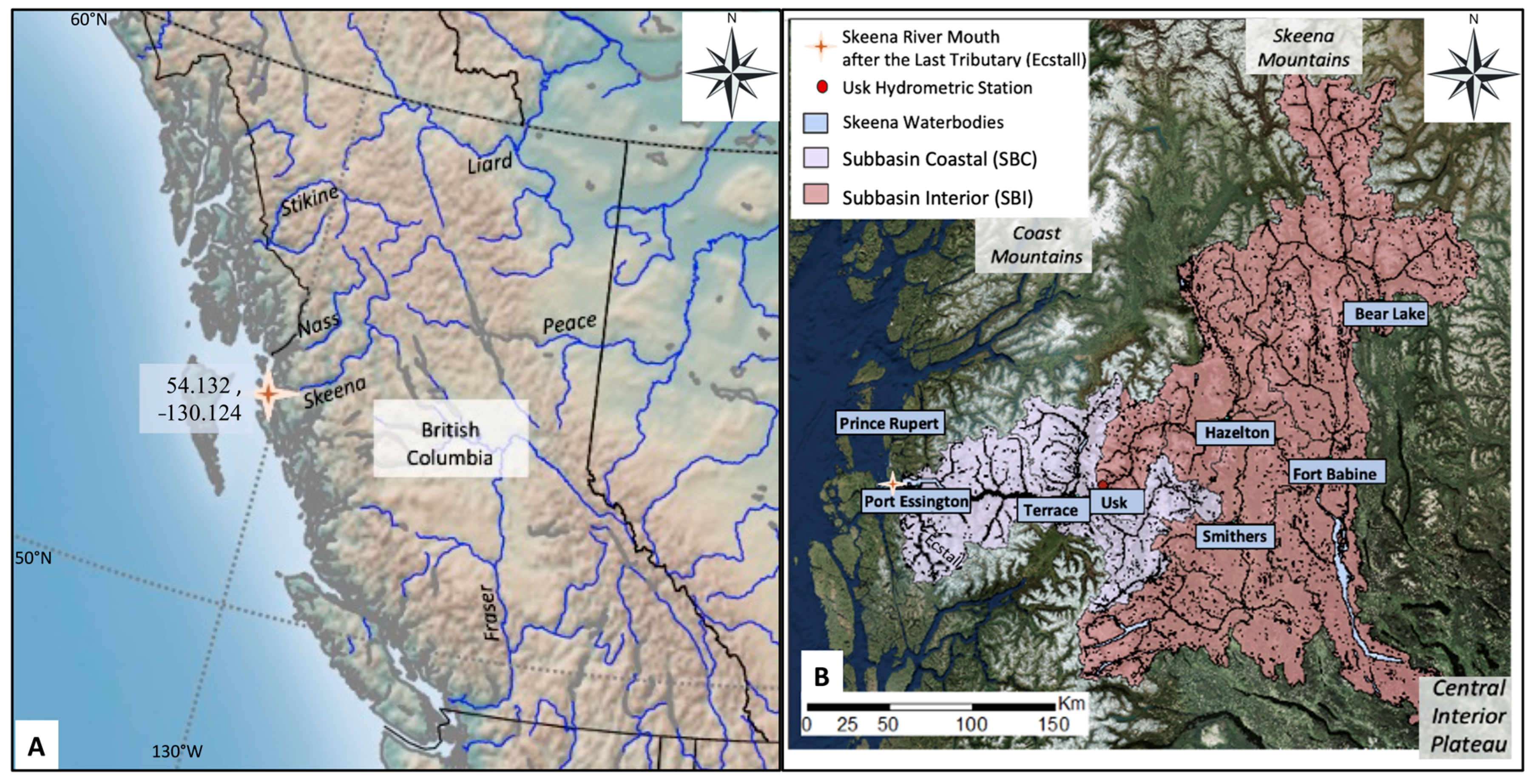
The Skeena River (Figure 1) empties into the Pacific Ocean after flowing 570 km south and southwest through the Skeena, Hazel, and Coast Mountains [12]. The Skeena River catchment covers an area of ~54,432 km2 [12] with 50% of the basin area at elevations above 1000 m. About 1197 km2 of the catchment are covered by glaciers, most of these located in the Coast Mountains [12]. The interior river valley is characterized by a wide (5–20 km) floodplain through low-grade metamorphic and sedimentary rocks. The coastal portion of the river valley downstream of Terrace (Figure 1b) is flanked by the steep, high-grade granitoid and gneiss complexes associated with the Coast-Cascade belt [16,17]. River valley fill reflects the recent glacial history of the Skeena watershed and consists of alluvial sediment overlying glacial till, especially in the interior portions of the catchment [18].
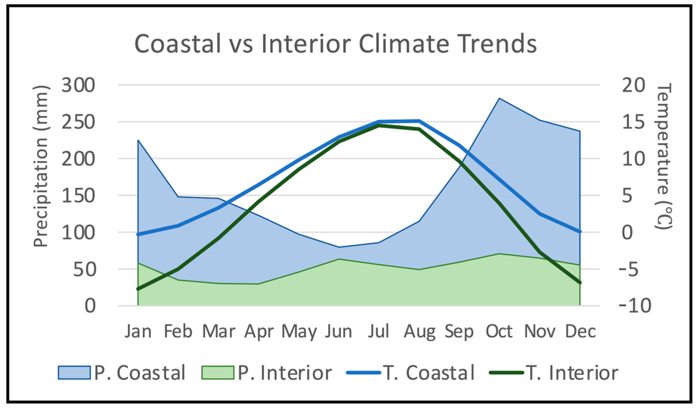
The climate governing the watershed varies between the interior and coastal portions of the watershed (Figure 2). The coastal sub-basin (SBC) receives higher precipitation and more moderate winter temperatures than the interior sub-basin (SBI). This is because high fall and winter precipitation occurs frequently in the coastal portion, while the interior portion is located in the rain shadow of the Coast Mountains [12,19]. Mean annual temperature in the Skeena River watershed has increased by 1.1 °C over the 20th century, particularly during the winter months [20]. During the same period, the average precipitation has increased by 10% and the glacial area has decreased by 6% at an estimated volume loss rate of −15.4 km3 yr−1 [20].
The Skeena River is gauged for discharge and water level in the interior portion of the watershed, but hydrometric stations on the main river branch of the river in the coastal area are missing. The hydrometric station furthest downstream is at Usk (for location, see Figure 1), which is located over 100 km upstream of the tidal limit defined by [12] and excludes ~22% of the watershed area. The measured annual mean discharge at Usk is ~900 m3 s−1 (rounded to the nearest 10 m3 s−1 using a 1981–2010 average [21]) and the highest flood event recorded (up to 2020) was in 1948 at 9340 m3 s−1 [21]. Along with a multitude of smaller creeks, roughly fourteen river tributaries join the Skeena River downstream of Usk [12]. These Coast Mountain tributaries are located in an area with substantial rainfall and retreating glaciers and potentially increase discharge and sediment load downstream of Usk significantly. The most comprehensive estimate of mean annual Skeena discharge is 2157 m3 s−1 based on monitoring data at Usk plus the contribution of four downstream gauged tributaries [22]. A past estimate of sediment load for the Skeena River is 11 G kg yr−1 with a yield of 260 t km−2 yr−1 using a watershed area of 42,000 km2 (corresponding to the area above Usk) [23]. An estimate of sediment discharge for the entire watershed is missing.
2.2. HydroTrend 3.0 Model Overview
HydroTrend 3.0 (herein referred to as HT or HydroTrend as suitable) uses a water balance model and semi-empirical relationships to estimate suspended sediment load, bedload, and water discharge at a river outlet based on inputs provided by the user that describe the watershed’s physical properties and climate [15]. The model has been successfully applied on studies across the globe, and is capable of reproducing a range of magnitudes in sediment loads and discharges [24,25,26].
Calculations are made over the total watershed area and are not tracked throughout the river network. Thus, results are produced at the drainage outlet. Input values for the model rely primarily on annual and monthly averages of input parameters of basin-wide conditions over any user-defined duration of interest (1–1000 s of years). Annual and monthly standard deviation (for climate inputs), distribution skewness (precipitation), and change per annum (for glacial equilibrium line altitude, or ELA) can be provided to account for temporal variation of the averaged inputs for the calculation of annual, monthly, and daily values.
As described further in Kettner and Syvitski [15], HydroTrend discharge and bedload are calculated at a daily time scale that can be post-processed further into user specified time intervals (e.g., monthly, annual). Discharge is calculated using a water balance that simulates precipitation, storage, reduction (e.g., evaporation), and release through components of rain (𝑄rain), snow melt (𝑄nival), glacial melt (𝑄ICE), groundwater discharge (𝑄ground), and total evaporation (𝑄eva) for the entire basin. Hypsometry and lapse rate along with climate inputs control a time-variable freeze line altitude used to estimate the proportion of precipitation stored as snow as well as the volume of glacial ice. Subsurface storage, transpiration, hydraulic conductivity of the dominant lithology cover are also considered as model inputs (see Appendix A section). A power law regression algorithm is applied within the model to estimate more extreme flood [15].
Bedload is calculated using a modified Bagnold’s equation:
where daily bedload () at the river outlet is calculated using the river bed slope at the river mouth (Sl), daily discharge (𝑄d), sediment density (), fluid density (), limiting angle of repose of sediments on the river bed (), and bedload rating () and efficiency () terms under the condition that stream velocity () exceeds the critical velocity needed to initiate bedload transport () [15].
Unlike the daily discharge and bedload, daily suspended sediment load () is calculated by first deriving the long-term suspended sediment load () for the user-defined simulation duration (1–1000’s of years)) contributed from overland/instream flow () and glaciers () [15]. Reservoir retention (trapping and residence time) of suspended sediment is calculated based on reservoir geometry and applied to the long-term calculation prior to deriving daily values. Using values of daily discharge over the simulation duration, a psi model calculates the inter- and intra-annual variability to apply to the long-term suspended sediment load to derive daily . Monthly values can then be derived within HydroTrend from the daily value calculations in post-processing [15].
Overland and in-stream contributions () to suspended sediment are derived empirically through a basin-wide approach by multiplication of long-term discharge (Q), maximum relief (R), drainage basin area (A), long-term basin-averaged temperature (T), B (a product of the lithology factor, trapping efficiency of reservoirs, and anthropogenic factor), and a coefficient of proportionality (0.02 kg s−1 km−2 °C−1) [15]:
Equation (2) is intended for basins with annual temperatures over or equal to 2 °C (see [15] and [27] for further details on the BQART method).
Glacial contributions () are derived through [15]:
where () is the ratio of precipitation turned to ice (based on the initial temperature, lapse rate, and hypsometry), () the total precipitation fallen on the glacial area, A is the total drainage area, b is the logarithm of the percentage of glaciers in the basin, and n is the total number of simulation years. Through a back calculation, is subtracted from an estimate of annual suspended flux based on watershed area and percentage of glaciers. The subtraction results are then averaged over the number of simulated years and multiplied by a ratio that determines the proportion of precipitation fallen, but not stored on the glacier, and which is available to transport sediment off the glacier. If all precipitation falling over the entire glacial area is stored, the ratio equals 1: the glacier is not melting and there is no discharge of water/sediment from the glacier (. = 0) [15].
For the purposes of clarity within the text, discharge (Q), suspended load (), bedload (), and suspended sediment concentration () results will be described using different subscript abbreviations depending on whether the presented results are referring to a (d) day (eg: ///etc.), a (m) month (eg: ), an (a) annum (eg: ), or an ()average of thirty years (eg: etc.) of HydroTrend outputs. refers to measured suspended sediment concentration and refers specifically to model-derived suspended sediment concentration. 𝑄ICE, 𝑄rain, 𝑄nival, 𝑄eva, , and , are the mean annual discharge derived from glacial melt, rain, snow melt, and total evaporation as well as the mean annual sediment load derived from the BQART and glacial contributions, respectively. Ground water contributions (𝑄ground) within model outputs are split between base flow contributions that are relatively constant to the river from the ground water table (𝑄base) and additional subsurface flow contributions (𝑄sub) that will vary depending on groundwater storage and subsurface storm flow.
2.3. HydroTrend Application for the Skeena: Approach, Inputs and Model Calibration
The results presented in this research are a cumulation of over 48 HydroTrend model runs (per sub-basin, epoch, climate input, and RCP) used to simulate changes in Skeena discharge and load. For the sub-basins, two different model set-ups were used for the calculation of suspended load and bedload of the Skeena River: (1) a one-basin approach (1-basin) was used to estimate bedload and (2) a sub-basin combination approach (2-sub-basins) was used to estimate suspended load. Discharge was calculated through both approaches for means of comparison. The rationale behind the 2-sub-basins approach is that the substantially contrasting climates and lithologies (key elements of Equations (2) and (3)) of the coastal and interior portions of the watershed are better accounted for when splitting the watershed into two basins, as opposed to averaging the contrasting conditions. The basins were divided at Usk, located on the eastern flank of the Coast Mountains, yielding an interior sub-basin (SBI) of 42,360 km2 and a coastal sub-basin (SBC) of 12,050 km2 (shown in Figure 1B). Results are than added to derive the suspended load at the river mouth. Using the hydrometric station data at Usk [21], validation of the SBI model output is possible. The sub-basin combination approach relies on the assumption that all material present at the sub-basin outlet will be carried to the final drainage sink. This can be plausible for the finer material; yet, it is well known that the coarser grains will change transport modes and eventually come to rest along the river course as slope decreases towards the outlet. With no known constraints on the proportion of bedload that falls out of transport between Usk and the river mouth, a simple addition of SBI and SBC bedload is problematic. Therefore, a 1-basin method, using the entire Skeena River reach and the outlet bed slope, is utilized for the calculation of bedload in this study.
HydroTrend results and simulations are run for the last climate normal (1981–2010) (the ‘reference period’), the current normal (2011–2040), and future climate normals (2041–2070, 2071–2100). Thirty-year epochs were chosen in alignment with the ECCC standard for calculating and releasing measured climate and discharge data. The last ECCC normal was computed and released from 1981–2010 (used during the validation of HydroTrend results) and the current normal including 2011 onward has not been released, as this period is still ongoing.
Each model run (per sub-basin or future epoch) requires a 47-line input file (Hydro.IN) along with basin hypsometry (Hydro.HYPS). For brevity, a list of the input variables, a brief explanation, and sources are given in the Appendix. A more detailed spreadsheet that includes details on the calibration using the long-term discharge data and the inputs chosen for each sub-basin is provided in the Supplementary Materials S1. All HydroTrend input files are also available on a GitHub repository (https://github.com/awild21/SkeenaHydroTrend, accessed on 23 December 2022 ).
Within Hydro.IN, only three input lines (temperature, precipitation (annual and monthly), and ELA) change between the future and reference simulations. For example, ELA change per year is used to calculate an evolving ELA over time at the start of each new epoch based on the reference ELA for each sub-basin (see Appendix and supplementary S1). Aside from climate and ELA inputs, all other variables (~44 input lines) remain constant across time, but vary depending on the sub-basin. For example, changes to groundwater storage over time are unknown (lacking data predictions) and thus, the same starting values for each sub-basin are used for the initial condition, maximum, and minimum ground water storage (described in the Appendix) for running each future scenario. HydroTrend over the simulation duration will depart from the initial storage condition (usual less than 1 month run up time) and will flag if the maximum or minimum groundwater condition were reached (no flags generated). Climate inputs have a dominant influence on the model outputs, are contrasted in the results, and are discussed in the following paragraphs.
For the reference period, Environment and Climate Change Canada (ECCC) [19] provides daily measured climate station data at multiple locations across the Skeena watershed. ECCC precipitation and temperature were averaged spatially across the sub-basin (monthly) or nearest to the river mouth (annually) as required for the model input. All temperatures should be input to the model at the elevation of the river outlet since a lapse rate is applied within the model [15]. Monthly, spatially averaged temperature data were corrected down to mean sea level (SBC) or to the base level of the river at Usk (SBI) using a lapse rate derived for the Skeena (see Supplementary Materials S1 and Appendix for further details). For simulations into the future, when no ECCC data are available, climate data from GCMs were extracted, averaged spatially (river mouth or sub-basin) and averaged into 30-year epochs. A lapse rate correction was performed on (sub)basin-averaged monthly data, following our approach for the ECCC data (see supplementary material S1).
When predicting temperature and precipitation in the current and future epochs (2011–2100), each GCM produces different climate scenarios based on different representative concentration pathways (RCPs) (see [28,29] for further details on RCPs and greenhouse gas trajectories). All of the GCMs presented are coupled earth system models, part of the Coupled Model Intercomparison Project Phase 5 (CMIP5) using the OASIS3 coupler, that differ by using different models and resolutions for simulating the Earth’s atmosphere, oceans, sea ice, continent, and fluxes [30]. The Pacific Climate Impacts Consortium (PCIC) [30]. Provides statistically downscaled daily climate scenarios for Western Canada (including minimum/maximum temperature and precipitation) at a gridded resolution of 300 arcseconds for up to 27 GCMs and multiple RCPs (for detailed methods and comparison of downscaling methods used by PCIC see [30,31]). PCIC orders the GCMs for a given region based on the Giorgi map regions [32], where the first and second GCM listed will offer the most contrast possible with diminishing differences between scenarios further down the list [30]. Twelve GCMs listed for the western North America region by PCIC capture 90% of the variance in temperature and precipitation predictions under RCP 4.5 [33]. The top three GCMs recommended for capturing the climate of the Skeena region were also among the top four GCMs used within a study in southwestern British Columbia to predict changes within the water resources of the Fraser River [34]. These GCMs were: CNRM_CM5-r1(referred to as CNRM), CANESM2-r1 (referred to as CANESM), and ACCESS1–0-r (referred to as ACCESS) (refer to [35,36,37] for details on the GCM model couplings and details for ACCESS, CANESM, and CNRM respectively). We retrieved climate data for these three GCMs and two RCPs, 4.5 and 8.5. A moderate (4.5) scenario was chosen to represent the more likely conditions [38] while the extreme, ‘worst case’ scenario [8.5] is shown for contrast. We compare model results for all three GCMs with model results using measured climate data in the validation section.
Model calibration involved running HydroTrend over SBI using the measured ECCC climate station inputs for the reference period with a range of inputs for a given variable and conducing a two-tailed test of the mean against the long-term 30-year-mean monthly () Usk hydrometric station results. The input variables that yielded the highest p-values were selected, or the most-cited for the region achieving a p-value over 0.9. Within the calibration for the Skeena, next to climate inputs (temperature and precipitation), glacial inputs and groundwater parameters had the largest impact on the discharge results (see input and calibration Supplementary Materials S1). All variables chosen using the long-term discharge yielded a p-value between measured and modelled discharge of more than 0.9. However, some model inputs do not affect the discharge and rather are used for the computation of suspended sediment and bedload. Due to lacking data, sediment was not included in the calibration, but will be compared to the available data from the Canadian Water Office [21] during the validation section and in a calculation of uncertainty/error around the sediment measurements (see Supplementary Materials S2).
To assess the uncertainty of the input variables concerning sediment loads, tests were conducted to examine the influence of these variables on computed suspended and bed load. One of the most important input variables with uncertainty controlling suspended sediment load derived from the BQART equation is the lithology factor [15,27]. According to the map by [27] (shown in the input Supplementary Materials S1), the Skeena watershed lies within a lithological factor of 1 (coast) and 2 (interior), due to the differing geology (in agreement with [17] descriptions). We adapted the values that are dominant on the [27] map for SBC and SBI, respectively. However, since there are limited sediment data for validation and it is unclear how representative they are, in the results, we will indicate what influence changing the factor by 0.5 (the resolution of the [27] lithological map) would have on our estimates of suspended load on the river mouth (shown in greater detail in the validation and uncertainty Supplementary Materials S2).
One of the most important input variables controlling bedload estimates is the delta plain gradient or bed slope at the river mouth. One estimate exists of 0.5 m km−1 [12] for the bed slope closest to the SBI outlet (near Terrace). This estimate, however, is located a distance upstream from the tidal limit [12] and from the actual river mouth in the tidally influenced estuary (see Supplementary Materials S1 for a map of the tidal limit). Measurements in Google Earth near the Skeena River tidal limit yielded slopes of ~0.333 m km−1. We have elected to use this value for our model simulations, but will indicate in our results what influence reducing or increasing the slope by 0.1 m km−1 has on our final bedload estimates (presented in detail in Supplementary Materials S2).
3. Validation
3.1. SBI Discharge and Sediment: Reference Period Model Predictions vs. Usk Measurements
Following the calibration of the model, 30-year measurements of discharge at Usk are compared to simulations of discharge for SBI using i) ECCC climate station data and ii) GCM input data. Very limited sediment data are available for the Skeena River. Measurements of at Usk station were conducted sporadically over only 13 days in various seasons in 1988–1992 by the Water Office Canada and are publicly available [21]. On these days, measurements were taken at 12 min intervals at five depths within the channel. To derive one estimate of ‘daily’ , all measurements were averaged across depths for a given day. Measurements at Usk were collected during a range of discharges between 156 and 3290 m3 s−1, representing freshet and non-freshet conditions providing a range of validation data suitable to test the model. In order to compare these values to daily modelled , all model values for the same month over the reference period under similar discharge (+/−50 m3 s−1) were extracted, averaged, and the standard deviation determined. For example, if one measurement was collected on May 15, 1990 at a discharge of 1000 m3 s−1, all modelled for days in May 1981–2010 with a discharge of 1000 m3 s−1 +/−50 m3 s−1 were extracted. This approach was used because 30-year average climate data was input to the model and a psi model used to produce variability between months and years (based on the 30-year mean), which prohibits an exact timing of 𝐶𝑠𝑑 to a given measurement day.
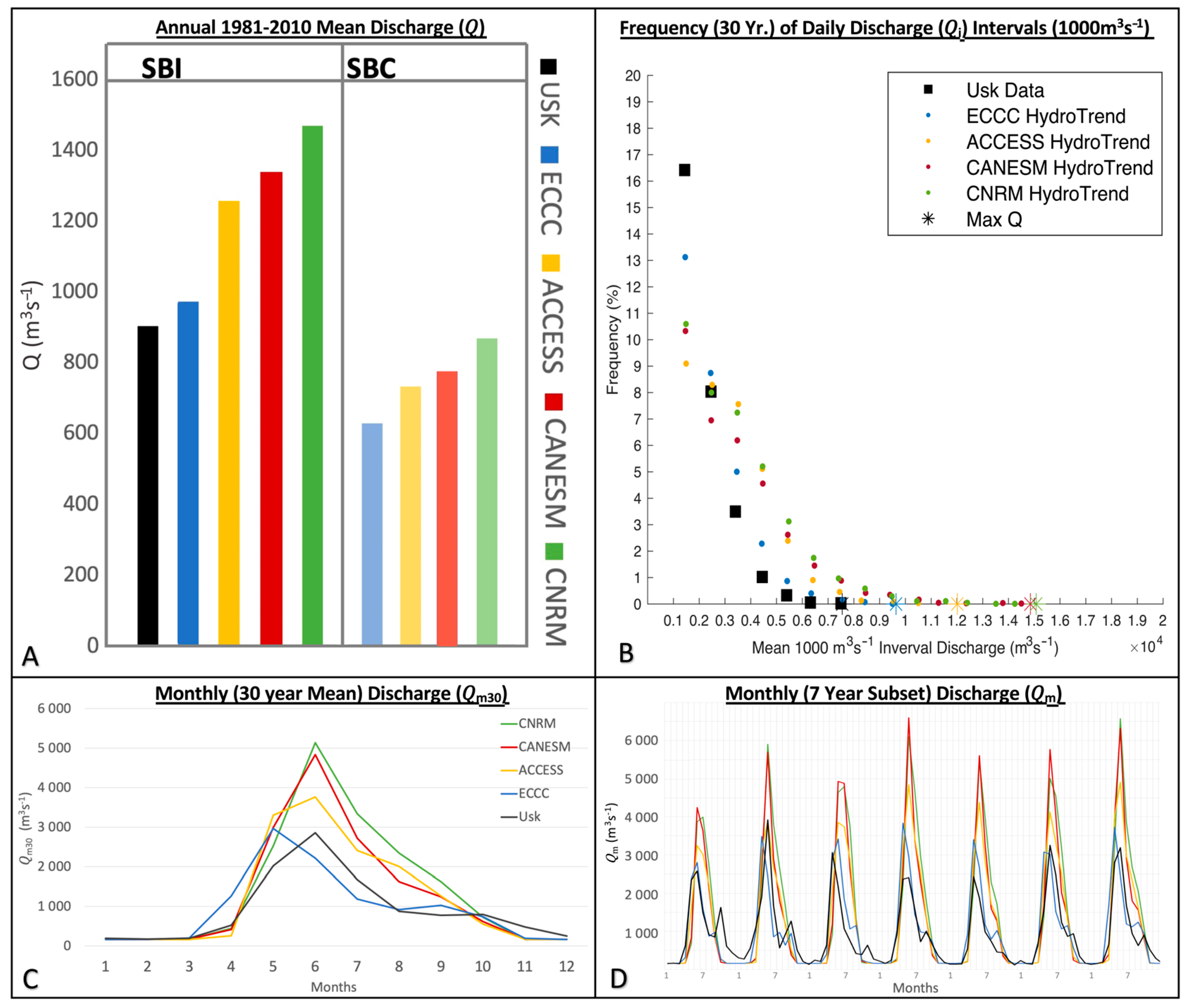
All model runs produce higher than that measured at Usk (~904 m s−3) during the same period (1981–2010) (Figure 3A). Estimates of increase for runs ACCESS, CANESM, to CNRM. This order of increase holds for model runs of the coastal sub-basin (SBC), for which no measurement data are available (Figure 3A). Comparison of measured and modelled (Figure 3C) shows overprediction of the annual river freshet by all model runs, except run ECCC, which predicts mean peak flows on average in May, rather than June. GCM Model runs overpredict from April–October and underpredict in the winter months (Figure 3C). A seven-year subset of measured and modelled (Figure 3D) shows that the underprediction may result because the GCM model runs are failing to predict a secondary peak in in the fall. Run ECCC on the other hand, which follows measured during this time period more closely, is at times capturing the secondary fall peak, and is also capturing the accurate timing of the freshet in some years (Figure 3D). A comparison of the frequency of daily discharge (𝑄d) events from measured and modelled data (Figure 3B) shows that the general overprediction of and , results from an overprediction of intermediate daily discharges (2000–5000 m3 s−1, as seen by the ‘hump’ in the otherwise exponential curves) and prediction of daily discharges > 8000 m3 s−1 that do not occur in the measurements. All models underpredict the frequency of daily discharges under 2000 m3 s−1.
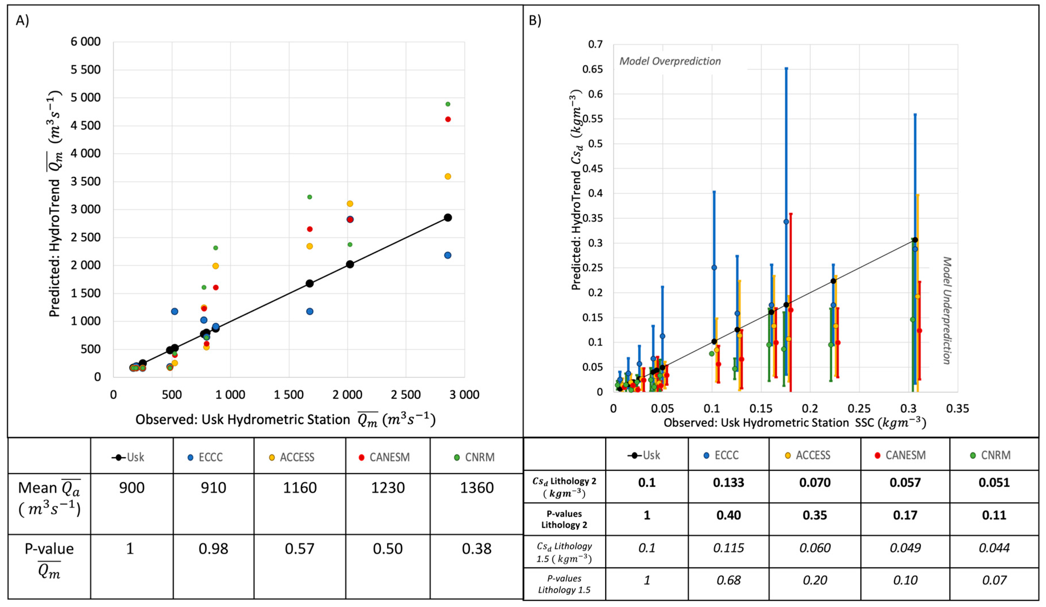
A two-tailed t-test comparing measured and modelled showed that p-values were 0.57, 0.5, and 0.38 for ACCESS, CANESM and CNRM, respectively. Out of the model runs, ECCC is closest to the measurements, with a p-value of 0.98 (Figure 4A). ECCC overestimated by only 1%. GCMs overpredicted the Usk discharge by 29% (260 m3 s−1), 37% (330 m3 s−1), 51% (460 m3 s−1) for ACCESS, CANESM, and CNRM respectively (see Supplementary Materials S2 for values). Since the CNRM scenario overpredicted the discharge by over 50%, we do not present future scenarios using CNRM in the results.
The lack of sediment concentration data is a limitation of this study and thus model results of daily are presented with error bars within one standard deviation to see if the measured values lie within this range (Figure 4B). Since data are limited, having the highest p-value capturing the mean does not mean that this is the most accurate representation of the long-term river data. However, the model should be able to capture the measured data within one standard deviation. All measured values fell within one standard deviation of the ECCC and ACCESS inputs using a lithology factor of 2. Modelled from run ECCC within one standard deviation reached into ranges well above the observed measurements, while the GCM runs tended to underpredict (Figure 4). The GCM models performed more poorly under the lithology factor of 1.5 whereas the ECC data achieved a higher p-value (see table in Figure 4B). In addition, the ECCC and GCM model results were better able to capture the measured values within one standard deviation range under factor 2 (see Supplementary Materials S2). Despite a lower p-value for the ECCC scenario, results for SBI using a lithology factor of 2 will be presented for the current and future 2011–2100 epochs since it matches more closely with the lithology factor map for SBI [27]. The difference between this, and a lithology factor of 1.5, is displayed in brackets as error/uncertainty within the historical results.
Thirty-year mean annual suspended sediment load ) (using a lithology factor of 2) are very close (205 kg s−1 from ECCC to 221 kg s−1 from CNRM in Supplementary Materials S2) among all model runs, likely because an overprediction of the frequency of intermediate discharges, paired with an underestimation of concentrations, leads to overall similar load estimates. However, there are no long-term suspended load data to offer comparison. Out of the runs using GCM climate data, run ACCESS is seen to perform best, followed after by run CANESM and run CNRM. Between the ECCC and GCM inputs, reducing the SBI lithology factor from 2 to 1.5 produced a reduction in suspended load of 30 (ECCC)-34 (CNRM) kg s−1 (Supplementary Materials S2). Between all model runs, the lithology factor of 1.5 produces a 17–18% decrease in sediment load from the lithology factor 2 results. SBC has only a 7% higher difference between the lithology factor 1 and 1.5 scenarios (19 kg s−1 for 245–264 kg s−1 using ECCC) (Supplementary Materials S2).
3.2. Skeena Watershed GCM Climate Predictions
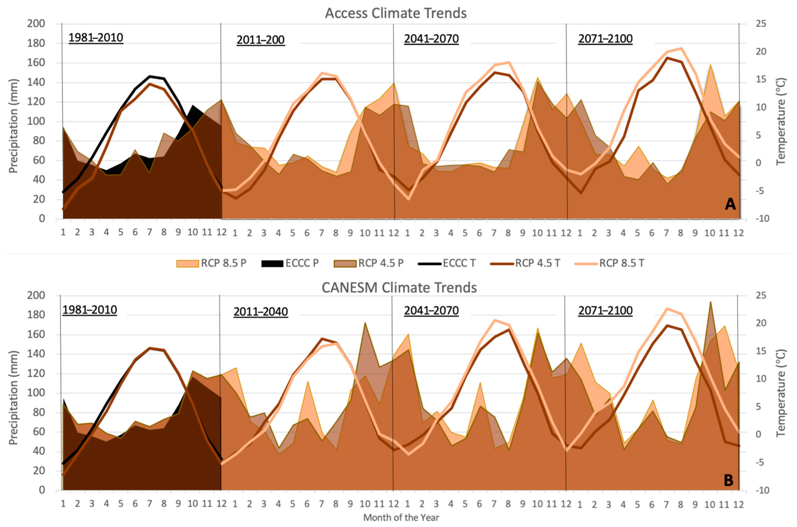
Basin-averaged, monthly temperature and precipitation normals (30-year averages) from GCMs for the reference (1981–2010), current (2011–2040) and future (2041–2070, 2071–2100) periods are shown in Figure 5 for the entire Skeena watershed. Also shown are the measured climate normals as derived from ECCC stations. During the reference period, temperature as derived from the ACCESS model appears consistently lower except for the winter months, while CANESM temperatures agree well with measured data (Figure 5, left). This is reflected in p-values of 0.64 and 0.87 for ACCESS and CANESM compared to the ECCC reference climate data, respectively. Precipitation from CANESM is, at times, up to 15 mm higher than ECCC data, while ACCESS precipitation fluctuates around the ECCC data, resulting in a higher p-value (0.94) than CANESM (0.64).
Both ACCESS and CANESM models predict increasing temperatures under RCP 4.5 and 8.5 scenarios, with maximum summer temperature increasing by 2–4° (RCP 4.5) or 5–6° (RCP 8.5) and minimum winter temperature increasing by 1° (RCP 4.5) or 3–4° (RCP 8.5). Both GCMs predict generally drier summers (1–5% drier for CANESM and 16–29% for ACCESS), while fall/winter precipitation increases (31–44% in CANESM and 10–17% in ACCESS). The CANESM model predicts the development of a more prominent peak in mid-summer precipitation as well as a more variable fall/winter precipitation compared to the ACCESS model (Figure 5). Differences between model outputs using RCP 4.5 or RCP 8.5 are generally higher temperatures, and more pronounced precipitation peaks under RCP 8.5, though shifts in timing also occur.
4. Results
4.1. Skeena River Mouth Reference Discharge and Sediment Load
Modelled discharge and sediment yield estimates at the Skeena River mouth for the reference (1981–2010) period are summarized in Table 1. The difference between using a slightly (within 0.5) lower (SBI: 2–0.5) or higher (SBC: 1 + 0.5) lithology factor based on the nearest values representing the area on the [27] map are shown in brackets for suspended load. Increasing or decreasing the river outlet gradient by 0.1 m km−1 is shown as a potential uncertainty in brackets surrounding the bedload estimate. Overall, the model results suggest that the larger, interior basin contributes more to mean annual discharge (), but less to mean annual suspended load () than the smaller coastal basin. This is because of the modelled high contribution to suspended load from glacial sources () in the coastal basin. Mean annual bedload ( derived from the 1-basin approach contributes to about ~22% of the total, mean annual sediment load (S) at the Skeena River mouth as per model result. Total Sediment Yield (Ys) for the watershed is estimated to be ~350 t km−2 yr−1. Values used to compute the best Skeena estimate within Table 1 are italicized and consist of the combination of SBI and SBC results/uncertainty for suspended load and the one whole basin results/uncertainty for bedload.
4.2. Skeena River Mouth Future Discharge and Sediment Load
4.2.1. Mean Annual Discharge and Sediment Load
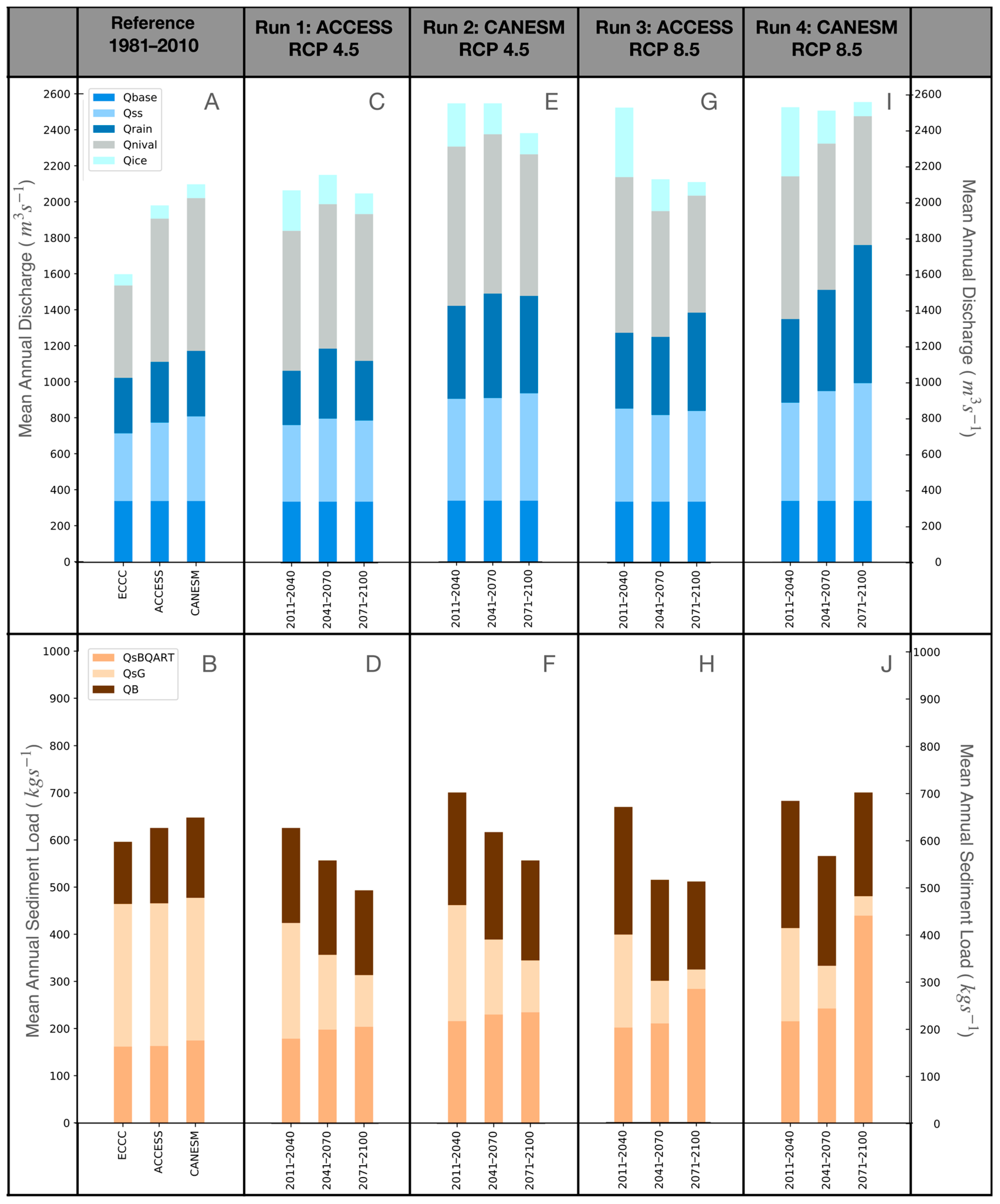
Mean annual discharge and sediment load for all four epochs are shown in Figure 6. The largest contributions to discharge in the Skeena in the reference period stem from snowpack melt () (28–39% across all runs). All model simulations predict a decrease in by the end of the century following an initial mid-century increase, except the ACCESS RCP 4.5 run, which predicts an increase in , if small (3%). Of those models predicting a decrease, RCP 8.5 models predict a higher decrease (by 15% (CANESM) and 18% (ACCESS)) than RCP 4.5 (7% (CANESM)). The lowest contributor to discharge is discharge from glacial melt () (4–15% across all runs). This contributor sees a rapid increase in the period 2011–2040 (current) compared to the reference period and a subsequent decrease in all simulations. The initial peak is more pronounced using the RCP 8.5 scenario than using RCP 4.5. By the end of the century remains higher than in the past (57% (ACCESS) and 54% (CANESM)) for RCP 4.5 and approaches reference values (only 3% higher (ACCESS and CANESM)) for RCP 8.5.
Apart from ACCESS run (RCP 4.5) which shows little overall change, model simulations predict an increase in by the end of the century when compared to reference values. CANESM runs predict a more drastic increase (by 49% for RCP 4.5 and 112% for RCP 8.5) than ACCESS runs (63% for RCP 8.5). While both simulations using RCP 4.5 decrease in the last period (2071–2100), simulations using RCP 8.5 predict a continued increase in . Discharge from subsurface flow () increases in all model simulations by the end of the century. CANESM runs predict a more drastic increase (27% (RCP 4.5) or 40% (RCP 8.5)) than ACCESS runs (4% (RCP 4.5) or 16% (RCP 8.5). The relative contribution of both and to overall discharge range between 15–30%, with experiencing a larger increase in relative importance than . As initial model input values for groundwater are held constant, discharge from groundwater flow () shows no variability throughout the century.
Overall, mean annual discharge ) is predicted to increase from reference values by the end of the century. CANESM predicts a 14% (RCP 4.5) to 22% (RCP 8.5) increase, while ACCESS predicts a 4% (RCP 4.5) to 7% (RCP 8.5) increase. Under RCP 4.5, appears to be on a decreasing trend towards the end of the century, while values seem to stabilize under RCP 8.5.
Model results for sediment load show that the contribution of suspended sediment from glaciers () decreases throughout the century, from approximately half of the total load to between 16% (CANESM) and 18% (ACCESS) of the total load under RCP 4.5 or 5% (CANESM) and 7% (ACCESS) under RCP 8.5. Suspended sediment derived from erosion in the catchment () increases in all model simulations throughout the century. CANESM runs predict an increase in by 33% (RCP 4.5) and 148% (RCP 8.5), while ACCESS runs predict an increase by 72% (RCP 4.5) and 138% (RCP 8.5). Combined, model simulations suggest that suspended load () decreases by about ~30% by the end of the century, except for CANESM run RCP 8.5, in which the increase in in the period 2071–2100 is able to compensate for the loss in and no change is observed.
All model simulations predict a rapid increase in bedload () in the period 2011–2040 (current) compared to the reference period and a subsequent decrease, resulting in an overall small increase in by the end of the century. The predicted increase is more drastic in RCP 8.5 than RCP 4.5 and in CANESM simulations compared to ACCESS. Overall, total load (combined suspended load and bedload, ) is predicted to increase in the period 2011–2040 (current) compared to the reference period driven by the rapid increase in bedload and only moderate decrease in suspended load. Following this peak, decreases by the end of the century. Whether this leads to an overall decrease compared to the reference period differs depending on the GCM used. CANESM runs predict a contrasting ~15% decrease in for RCP 4.5 and ~10% increase under RCP 8.5, driven by the increase in bedload and increasing under this scenario. ACCESS runs predict a decrease in by up to 20% driven by the decrease in .
4.2.2. Mean Monthly Discharge and Sediment Load
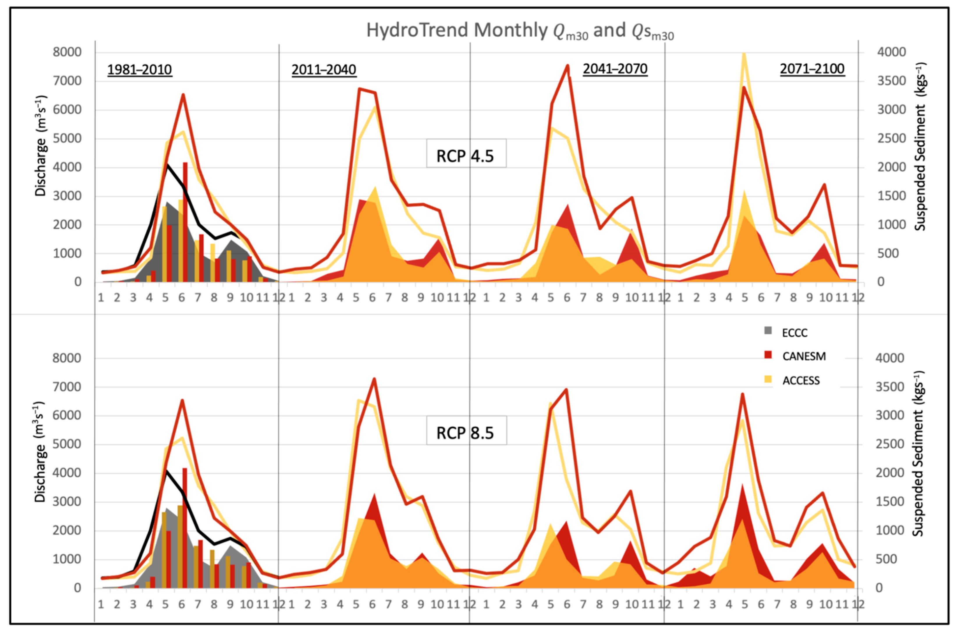
Analyzing the seasonal trends can provide additional details on shifts in the timing of future river discharge and load. Figure 7 depicts modelled mean monthly discharge () and suspended sediment load (for the four time periods. All model runs predict a shift towards a more bimodal pattern in and by the end of the century due to an increase in the secondary fall peak and decrease in mid-summer values. The fall peak is more pronounced in CANESM simulations than in ACCESS simulations for both variables. Also observed in all simulations is a shift in timing of the primary peak from June to May by the end of the century. The magnitude of peak flow fluctuates under RCP 4.5 with no clear trends, but decreases for both GCM runs under RCP 8.5 following an initial increase in 2011–2040. Peak does not display a similar trend.
5. Discussion
5.1. Skeena River Sediment Yield in Context
Remote sensing along the British Columbian coastline has shown that the highest sediment concentrations occur in sediment plumes at the mouths of the Fraser, Skeena, and Stikine rivers [39]. Our best model estimates give a mean annual discharge of ~1500 m3 s−1 and a mean annual sediment load of 18.9 (+1.9/−2.3) G kg yr−1 (Table 1). This discharge estimate is below previous estimates of 2157 m3 s−1 [22], while sediment load is larger than the only previous estimate available (11 G kg yr−1 [23]), likely due to the previous neglection of the coastal sub-basin.
For rivers in mostly non-glaciated watersheds in BC, [9] predicted an upper and lower envelope or ‘main trend’ of specific suspended sediment yield per basin area, invoking the importance of the legacy of glacial deposits and erosion in river valleys over modern hillslope processes. Accordingly, specific suspended sediment yield increases with drainage area up until 30,000 km2 and then decreases for larger basins. For context, the well-studied Fraser River to the south (Figure 1) drains the largest basin area within British Columbia (250,000 km2) with a mean annual discharge of 3410 m3 s−1, a mean annual suspended load of 17 G kg yr−1 [40] (and a resulting specific suspended sediment yield of 68 t km−2 yr−1). Our modelled Skeena River (basin area of 54,410 km2) specific suspended sediment yield is 250–280 (270 best estimate) t km−2 yr−1 and lies well within the envelope of specific suspended sediment yields of this size (95–400 t km−2 yr−1, [9]). This may be surprising given the large amount of estimated modern glacially derived sediment in the Skeena (~65% of the total suspended load, most of which from the coastal sub-basin) that is usually thought to cause deviations from this main trend [41]. Calculating specific sediment yield for non-glacial sources only, yields 96 t km−2 yr−1 and is at the lower limit of the range specified by [9]. The Fraser River similarly falls at the lower end of the range specified for rivers of its size (70–200 t km−2 yr−1, [9]). Recall that an attempt was made to consider the Pleistocene glacial legacy of till deposits within the Skeena by using the higher lithology factory (more available/erodible sediment) within the interior sub-basin that may aid in ensuring that the Skeena estimates fall within the Church and Slaymaker [9] envelope. Given the topographic complexity of the Skeena River (the river travels through a secondary mountain range shortly before reaching the Pacific), these results are encouraging in that our predictions for the Skeena fall within the bounds described by [9] both when including and excluding the modern input from glaciers.
Total specific sediment yield (including bedload) is 350 t km−2 yr−1 according to our model results. Bedload accounts for ~22% (+/−6%) of this total yield, a larger proportion than the 10% commonly attributed to bedload in many rivers worldwide [42,43]. In the Pacific Northwest, the similarly sized Susita River (Alaska), for example, has a total sediment yield of 560 t km−2 yr−1 with a bedload contribution of 29 t km−2 yr−1 (5%) [44]. Susita River may be less steep in its final reaching due to a wide flood plain (visible in Google Earth) in comparison to the Skeena that is closely constrained (almost fjord-like) by mountains on either side, but this is uncertain. Higher bedload proportions do exist, particularly in mountainous catchments (>30%, [45,46]), and the Skeena River runs through the steep topography of the Coast Mountains in its final reaches. Still, our model results may be an overestimation of bedload yield and very greatly depend on where one defines the river mouth and delta slope. Thus, bedload estimates should be treated with caution in the light of uncertainties around the bed slope and tidal influence in the final river reaches.
5.2. Future Changes in Discharge and Sediment Load
Projected changes in temperature and precipitation by the end of the century are expected to influence the hydrological regime in the Skeena River watershed. Generally, changes in temperature are thought to influence the timing of runoff (e.g., timing of freshet peak), while changes in precipitation are thought to affect maximum snowpack accumulation and runoff volume [47]. The Skeena River today exhibits a hybrid hydrological regime, with a freshet discharge peak in late spring due to snow-melt and a secondary peak in late summer/fall due to increased fall precipitation in addition to glacial melt [21]. Hybrid hydrographs (opposed to a snow melt dominant hydrograph with a single prominent discharge peak) show two distinct discharge peaks, one that is snow melt (freshet) derived (typical of the interior of British Columbia) and one that is rain (fall or winter storm) driven (typical of coastal British Columbia catchments). Generally, our results predict an increase in mean annual flow by the end of the century, caused by an increase in glacial ice melt, and an increase in discharge from rain and subsurface flow. This concurs with an earlier onset of the freshet peak. These observations are consistent among all GCMs and RCPs chosen. Several modelling studies that have examined changes in the hydrological regime of the Fraser River (southern BC) have shown similar predictions where mean annual discharge increases throughout the century, accompanied by an earlier onset and decrease of the freshet peak [48,49].
Shifts in timing of the freshet peak lead to/reflect a reduction in the length of snow accumulation season. However, results vary, depending on rising precipitation and temperature fluctuations, as to how this is expressed within the discharge hydrograph and mean annual flow. Initially, Skeena discharge predictions from snow increases mid-century, associated with an increase in winter precipitation, particularly in CANESM simulations. This appears to moderate the effect of rising temperatures on snowpack accumulation. Such observations have also been made for other high elevation mountainous regions where the projected increase in precipitation is large [6,50,51]. Near the end of the century, snowpack melt follows a decreasing trend, suggesting that increased precipitation may no longer be able to offset rising temperatures [52]. The magnitude of the spring melt freshet peak is predicted to decrease only under one, more extreme RCP 8.5 scenario. Results for model runs using RCP 4.5 show no consistent trend among the epochs. Such lack of consistency is indicative of the variability in spring runoff that is strongly influenced by fluctuations in annual spring temperature and precipitation. The highest floods can be expected when high temperature anomalies in spring melt season coincide with heavy rainfall causing rain on snow events. For example, the latest flood warnings in the Skeena region of BC were issued in 2022, when a cool and wet winter/early spring season with heavy snowpack accumulation was followed by heavy rainfall and a rapid increase in temperature [53].
Skeena predictions show a shift towards increased bimodality, with an increase in secondary fall peak magnitude and a decrease in summer discharge. This is related to an increase in fall precipitation as well as on average drier and hotter summers, particularly in the CANESM simulations, for which these bimodal patterns are more distinct. The matches with recent events in the summers of 2021 and 2022 in BC have shown that this average increase in summer temperature is frequently accompanied by high temperature anomalies, or heat waves [54], that can induce additional variability in the hydrological conditions and add stress to fisheries (e.g., [55]). Within the Fraser River, winter and spring runoff are predicted to increase with ongoing climate changes while summer runoff will decrease, leading to a shift from snow-dominant to hybrid regimes in the Coast Mountains and shifts from hybrid to rain-dominated regimes in the central plateau [48]. Within the Skeena, a possible shift towards a rain-dominant regime such as observed by [48] may occur beyond the century, but is not yet prevalent throughout this century based on our model results.
Examining the contributions to discharge, over the four time periods studied, illustrates that the largest increase in discharge for most models occurs from the reference period (1981–2010) to the current epoch (2011–2040), due to the sudden change of discharge contributions from ice or glacial melt. Such changes are well underway and have already been documented in many studies [6,50]. From 2011–2040 onwards, both snowpack and glacial melt follow a decreasing trend in the model results.
Future changes in sediment load are more complex, especially in the Pacific Northwest, where glacial legacy may at times overshadow recent fluvial activity [41]. The large amount of sediment derived from glacial sources, however, makes the Skeena susceptible to climate change. All our model simulations predict a rapid decrease in glacial sediment load, a trend that will likely continue beyond this century as glaciers diminish in size. Predicted changes to the non-glacial sediment load, are not consistent among our simulations, which depend largely on differing precipitation predictions between the RCPs. Increased precipitation and warmer temperatures throughout the century lead to an increase in basin-derived suspended sediment, which has been attributed to higher runoff and higher sediment availability in other river basins in the Pacific Northwest (e.g., [56,57]). Analysis of the daily model outputs suggests that this increase is accompanied by a tendency towards more episodic rain events and more extreme fluctuations in daily discharge. These predictions are consistent with observations within the past few decades or predictions of more intense and episodic storms and atmospheric rivers followed by periods of drought in BC (e.g., [58,59,60]). The increase in basin-wide-derived suspended sediment predicted by our model may in part be driven by the more episodic nature of discharge events. This increase cannot compensate for the loss of glacial sediment, except for the simulation using CANESM GCM forcing and RCP 8.5, which predicts the largest amount of increase in rainfall, compared to the other runs. A slight increase in the overall suspended load from 2041–2070 to 2071–2100 in the simulation using ACCESS GCM forcing and RCP 8.5 may point to a delayed compensation of the loss of glacial sediment beyond this century. Bedload initially increases, but follows a decreasing trend towards the end of the century concurrent with our predictions of discharge.
These results are carefully scrutinized, a variety of scenarios are given, and a validation of results provided wherever possible; however, a modelling approach does come with assumptions and some inconsistencies which are explained here. Though the validation showed that models using GCM forcing overpredict discharge, particularly from snow for 1981–2010, the trends observed are consistent among model runs. This overestimation could lead, however, to shifts in timing of the real-world scenario compared to our observations. Glacial melt, for example, could peak and subsequently decrease earlier or later in the century and the snowpack contributions could more rapidly or more slowly decline. In addition, there are a number of factors that have not been considered in our model. Firstly, groundwater processes are directly affected by changes in temperature and precipitation, which may cause changes in the contribution of groundwater to discharge, particularly in the summer [61]. Few data are available regarding groundwater processes (except for immediately around select communities) and future changes therein for the Skeena watershed. The model predicts that base flow and subsurface flow account for ~0.3–0.35% of the current discharge and warrants further study within the watershed. Changes in discharge are also caused by changes in vegetation or soil characteristics (human- or climate-induced) and can at times moderate effects of changing temperatures and precipitation [62]. Changes in vegetation or land use will also affect riverine sediment load and need to be considered for a holistic understanding of future change [63,64,65]. For example, increased mining, forest fires, landsliding, deforestation, or agriculture could all increase concentrations in a river [64], but are not accounted for by the model aside from potentially changing lithology or anthropogenic constants. Beyond the century, based on the observed trajectory of a decrease in glacial load and bedload, hillslope and valley-fill erosion driven by increasing precipitation and temperature will likely become the dominant drivers of Skeena River sediment load.
6. Conclusions
- This study examined fluvial discharge and sediment load and changes thereof due to climate change of a mountainous river in the Pacific Northwest (Skeena River, BC). For 1981–2010, using measured ECCC climate station inputs, mean annual discharge of the Skeena River is predicted at 1500 m3 s−1 with a mean annual suspended load of 14.7 + 0.6/−1 G kg yr−1 and a sediment yield of 350 t km−2 yr−1. The largest contributor to suspended sediment is derived from glacial sediment.
- Future changes in the climate of the Skeena Basin using GCM inputs predict an increase in summer and winter temperatures, and a development towards drier summers and wetter fall/winter periods by 2100. As a consequence, mean annual discharge is projected to increase rapidly during the period 2011–2040, driven by increased ice melt. Discharge then plateaus or decreases toward the end of the century, as contributions by snow and ice decline and those from rain and subsurface flow increase. An increase in seasonality of discharge occurs, with a distinct late summer secondary (in addition to the primary freshet in spring) flow peak developing due to high fall precipitation. A shift towards earlier peak flow is observed in all model simulations. Sediment load contributed by glaciers is projected to decrease by 64–69% (RCP 4.5) to 87% (RCP 8.5) by the end of the century. Rising precipitation increases the basin-wide mobilization of sediment from overland and instream contributions, particularly towards the end of the century. Bedload increases initially but continues towards the end of the century with a downward trend matching the discharge trend.
- Our findings highlight the sensitivity of mountainous river basins to climate change and stipulate a transition towards rain-dominant fluvial regimes with a loss of glacial ice and snow pack at high altitudes. Our results do not show that such a transition is completed within the Skeena by the end of the century (some contributions from glacial ice and snow pack melt remain by the end of the century). Future work should examine whether this shift is accompanied by changes in transported grain size and stored alluvium, which in turn can alter the stability of riverine and coastal habitats.
Supplementary Materials
The following supporting information can be downloaded at: https://www.mdpi.com/article/10.3390/w15010167/s1. Two supplementary files area available: (1) detailing the model inputs and discharge calibration; (2) detailing the validation and uncertainty/error calculations for SBI and the best estimate for the Skeena River mouth.
Author Contributions
Conceptualization A.L.W., D.G.L., S.F.; methodology, A.L.W., D.G.L., S.F.; validation, A.L.W.; formal analysis, A.L.W.; investigation, A.L.W.; resources, A.L.W., E.K., D.G.L.; data curation, A.L.W.; writing—original draft preparation, A.L.W., E.K; writing—review and editing, A.L.W., E.K., D.G.L., S.F.; visualization, A.L.W.; supervision, E.K., D.G.L., S.F.; funding acquisition, E.K., A.L.W. All authors have read and agreed to the published version of the manuscript.
Funding
Eva Kwoll received funding through a NSERC Discovery Grant. Amanda Wild was a 2019–2020 NSERC- Alexander Graham Bell Canada Graduate Scholarships-Master’s recipient or received a fellowship from the Department of Geography at the University of Victoria while the majority of this research was conducted. During the final, editing phase of this research, Amanda Wild received funding from the European Union’s Horizon 2020 research and innovation program under the Marie Sklodowska-Curie grant agreement No 860383.
Institutional Review Board Statement
Not applicable.
Informed Consent Statement
Not applicable.
Data Availability Statement
Additional Model inputs and metadata from this study can be found at: https://github.com/awild21/SkeenaHydroTrend accessed 23 December 2022.
Acknowledgments
We would like to acknowledge the Tsimshian people on whose unceded traditional tribal territory the Skeena Estuary is located. This work was conducted as part of the master’s research of A.L.W and would like to thank fellow colleagues and professors at the University of Victoria Geography Department and at the Pacific Geoscience Center. We would also like to thank the Pacific Climate Impacts Consortium (PCIC) for providing access to GCM model raster’s and the CSDMS community, especially Albert Kettner and Irina Overeem, for answering questions and for making HydroTrend available for researchers around the world.
Conflicts of Interest
The authors declare no conflict of interest. The funders had no role in the design of the study; in the collection, analyses, or interpretation of data; in the writing of the manuscript; or in the decision to publish the results.
Appendix A

Table A1.
HydroTrend Model Input Summary.
| Input Parameter Name | Description | Method of Calculation for the Skeena Basins |
|---|---|---|
| General Overview Notes | For more description of HydroTrend please consult [15,66] | Consult the Supplementary Materials for greater detail on the methods, the input values for each sub-basin, and for the calibration. Input files can be found on GitHub: https://github.com/awild21/SkeenaHydroTrend accessed 23 December 2022. Except hypsometry (Hydro.HYPS), all values described in this Appendix are included within Hydro.IN. |
| Hypsometry | The Hydro.HYPS file contains the area (km2) at each 50-m elevation bin. | The British Columbia digital elevation model (DEM) [67], was clipped for each sub-basin and binned into 50 m intervals to produce a hypsometry file for each sub-basin. The watershed drainage defined by [68] were used to derive sub-basin areas. |
| Mean annual Temperature (°C), temp. change/year, & temp. σ; Annual Precipitation (m), change/year, & σ. | Annual climate values at the basin mouth were computed using GCM data or ECCC stations. | Future GCM: GCM data were downloaded from [30], averaged over the time interval desired (30 years) for each basin, and clipped in a 2 km buffer at the basin outlet. Reference ECCC: For the reference SBC and SBI, the nearest up and downstream ECCC stations [19] to the river outlet were averaged to produce the basin mouth climate. For all of the following inputs described in this Appendix, the inputs for the whole Skeena basin (WS), were calculated through a spatial average (based on the area of SBC (~0.22) or SBI (~0.77) over the total area) of SBI and SBC. |
| Rain Mass Balance Coefficient (RC), Distribution Exponent (RD), & Distribution Range (RR) | The RC coefficient is used to scale for a large basin-wide difference in precipitation [66]. A RD is applied to specify the skewness of the default Gaussian distribution and create realistic tails for daily precipitation events. The RR defines the width of the skewed Gaussian distribution and lies between 0 and 10 [66] | An analysis of ECCC station precipitation curves across the Skeena basin, and a comparison to inputs from [19,25,69] informed value selection. |
| Constant annual base flow (m^3/s) | Constant annual base flow was derived from the mean minimum monthly flow each year at Usk hydrometric station [21] averaged over 1981–2010. | |
| Monthly climate variables of mean temperature (T) in °C, T σ, total monthly Precipitation (P) in mm, and P σ. | Historic: For each basin, daily ECCC climate station variables [19] were averaged monthly for stations with over ten years of data available over the 1981–2010 period. Climate inputs for the whole Skeena were calculated through a weighted average of SBC and SBI. Temperature was adjusted using the lapse rate [70] from the mean elevation of the stations/GCM to the elevation of the basin outlet. Future: For 2011–2100, for each GCM and RCP, statistically downscaled climate scenarios raster grids for mean T maximum (TMax), T minimum (TMin), and P were downloaded from the Pacific Climate Impacts Consortium [30] under 5 year increments, averaged into a 30 year mean raster in Matlab, and clipped over the basin area in ArcGIS. TMax and TMin are averaged to produce the T mean. Temperature was adjusted using the [69] lapse rate from the mean elevation of the stations/GCM to the elevation of the basin outlet. | |
| Lapse rate (°C/km) | The Syvitski et al. [69] graph was used to estimate lapse rate based on latitude. | |
| Starting glacier ELA (m) and ELA change per year (ma−1) | Mean starting Equilibrium line altitude for the basin. | The mean glacier ELA was calculated using a dataset retrieved from the Rudolf Glacier Inventory [71] that was developed through an analysis on 2004–2006 glaciers within British Columbia (BC). A study on glacier mass balance in northern BC and Alaska under different climate change scenarios [72] was used to derive ELA change per year. |
| Dry precipitation evaporation fraction (ICE) | The ICE falls between 0.0 and 0.9 and is used to estimate the percentage of snow and ice that will be evaporated [66] | Lintern and Haaf [25] have run HydroTrend over the Liard basin further north in British Columbia with an estimated ICE of 0.27. The Liard ICE was scaled for the Skeena based on the ECCC central station’s [19] percentage of the year without precipitation of the two basins. |
| Canopy interception alpha g (mmd−1), beta g (-). | The model uses the canopy interception parameters to estimate how much precipitation is reaching the ground and contributing to runoff [66] | The canopy interception values of −0.1 and 0.85 was applied for the Skeena watershed based on recommendations on the CSDMS website [66]. |
| Groundwater pole evapotranspiration alpha_gwe (mmd−1), beta_gwe (-). | HydroTrend applies the groundwater pole evapotranspiration parameters to estimate the amount of water from the ground being taken up by plants and brought into the atmosphere by evapotranspiration [66] | The recommended common values of 10 mm day−1 and 1 were used for the Skeena [66]. |
| Delta Gradient (m/m) | The delta plain gradient in m/m is the average slope of the riverbed approaching the delta mouth. | Delta plain gradient was derived from values in [12] or measured in Google Earth. |
| River basin length (km) | The River basin length for each sub-basin was measured in ArcMap using Global Mapper satellite imagery and the National Hydro Network of rivers and streams layer [68]. | |
| Mean volume (km3), altitude (m) or drainage area of reservoirs (km2) | Using the National Hydro Network [68] for lakes and reservoirs along with the BC DEM [67], the average altitude and area for all of the lakes and reservoirs were calculated. Mean lake depth was estimated based on available data from [73,74]. | |
| River mouth velocity coef.(k) and exponent (m) (v = kQm); River mouth width coef. (a) and exponent (b) (w = aQb). | River mouth velocity and width coefficient were calculated using channel width, depth, velocity, and discharge based on the hydraulic geometry formulas developed by Leopold & Maddock (1953) [75]. | Leopold & Maddock [75] describe common exponents at a river’s mouth as 0.5, 0.1, and 0.4 for b, m, and f, respectively. For SBI, mean discharge and water level were calculated using Usk station data from ECCC [21] and channel width was measured using Google Earth Satellite imagery. For SBC, the discharge was derived from BC Ministry of Environment [22] discharge summation. In addition, at the start of the river mouth, prior to substantial tidal inundation, depth was taken from the nearest Canadian Hydrographic Service bathymetry. Channel width was measured in ArcMap. Velocity was derived from the discharge divided by the width and depth according to hydraulic geometry. |
| Average river velocity (ms−1) | Velocity was derived from the 1981–2010 mean discharge at Usk hydrometric station [21] divided by the product of the mean water level from Usk [21] and mean channel width measured using Digital Globe satellite imagery. Since Usk was centrally located within the Skeena watershed and due to limited hydrometric data, the velocity at Usk was used as the average velocity for the river. | |
| Maximum/minimum Groundwater storage (m3) | A global data set by Webb et al. (2000) [76] displays a raster of estimates of global soil texture and derived water holding capacity across the globe per arc second grid blocks, was used to estimate the minimum and maximum groundwater stored within the Skeena. Within ArcGIS, the minimum and maximum storage for each pixel type was multiplied over each pixel area and added together for each Skeena [68] sub-basin. | |
| Initial Groundwater storage (m3) | The initial groundwater storage was set the mean condition between the maximum and minimum groundwater storage of the model to reduce the model run up time. | |
| Ground water (subsurface storm flow) coefficient (m3s−1) and exponent (unitless) | SSF coefficient and exponent required by the model, the coefficient and exponent were adapted from those used by Linter and Haaf, (2014) [25] over the Liard basin. The Liard basin has relatively comparable surficial material as the Skeena [17,27]. However, Skeena and the Liard basins are very different in size. Therefore, the SSF and total area for the Liard basin [25] was scaled to match the area of the Skeena and each sub-basin used within the model. The SSF exponent was set to one, as was the exponent used within all sub-basins of the Mackenzie [25]. | |
| Saturated hydraulic conductivity (mmday−1) | Proportions of surface lithology for the Skeena (see [17]) were estimated for each sub-basin. Applied to the soil textural and related saturated hydraulic conductivity chart shared on the CSDMS website [66], a hydraulic conductivity value of 121.91 mm day−1 was used to describe the glacial till substrate. A medium texture of silt with a hydraulic conductivity of 36. 55 mm day−1 was chosen to represent alluvium. The marine sand and complex material were attributed a loam sand- sandy loam texture of 364.95 mm day−1. Based on the CSDMS hydraulic conductivity table, a rough estimate of 1 mm day−1 was applied to the bedrock. A weighted average based on the proportion of the sub-basin covered by each landcover type based on surface lithological maps and descriptions [12,17] was as used to compute the total sub-basin average hydraulic conductivity. | |
| Longitude, latitude at river mouth. | Latitude and longitude retrieved from ArcMap. | |
| BQART Equation: Lithology factor from hard (max. 0.3) to weak (min. 3) material. | A lithology factor of 1 (SBC) to 2 (SBI) depending on the Skeena basin was chosen based on a classification scheme defined by Syvitski and Milliman (2007) [27]. A lithology factor of 1 is intended for areas consisting of volcanic rock or a mixture of hard to soft lithologies [27], typical for the Skeena Coast [17]. A lithology factor of 2 represents a greater proportion of glacial till and clastic sediments [27], typical for the Skeena Interior [17]. A lithology factor of 1.5 represents softer-mixed lithology [27]. | |
| BQART Equation: Anthropogenic factor (0.5–8) of human disturbance on the landscape | Syvitski and Milliman (2007) [27] have defined the anthropogenic factor on a global scale based on population density and gross national product (GNP) per capita. For basins around dense cities in the United States and Europe, a factor of 0.5 is recommended due to a high population density, GNP/capita, and human influence on soil erosion. A factor of one was displayed for most of the globe and was described as areas with a low human footprint or a mixture of soil erosion and conservation drivers. Basins in parts of Asia, with a high population, but low GNP/capita or those at their historic peak of forestation of open pit mining are recommended with a value of 2 [27]. Although the Skeena is influenced by forestry, the impacts appear lower than those in other basins on a global scale. Therefore, a factor of 1 was chosen for the Skeena. |
References
- Syvitski, J.P.; Kettner, A. Sediment flux and the Anthropocene. Philos. Trans. R. Soc. A Math. Phys. Eng. Sci. 2011, 369, 957–975. [Google Scholar] [CrossRef] [PubMed]
- Bauer, J.E.; Cai, W.-J.; Raymond, P.A.; Bianchi, T.S.; Hopkinson, C.S.; Regnier, P.A.G. The changing carbon cycle of the coastal ocean. Nature 2013, 504, 61–70. [Google Scholar] [CrossRef] [PubMed]
- Battin, T.J.; Kaplan, L.A.; Findlay, S.; Hopkinson, C.S.; Marti, E.; Packman, A.I.; Newbold, J.D.; Sabater, F. Biophysical controls on organic carbon fluxes in fluvial networks. Nat. Geosci. 2008, 1, 95–100. [Google Scholar] [CrossRef]
- Milliman, J.D.; Syvitski, J.P.M. Geomorphic/Tectonic Control of Sediment Discharge to the Ocean: The Importance of Small Mountainous Rivers. J. Geol. 1992, 100, 525–544. [Google Scholar] [CrossRef]
- Pepin, N.; Bradley, R.S.; Diaz, H.F.; Baraër, M.; Caceres, E.B.; Forsythe, N.; Mountain Research Initiative EDW Working Group. Elevation-dependent warming in mountain regions of the world. Nat. Clim. Chang. 2015, 5, 424–430. [Google Scholar] [CrossRef] [Green Version]
- Stewart, I.T. Changes in snowpack and snowmelt runoff for key mountain regions. Hydrol. Process. Int. J. 2009, 23, 78–94. [Google Scholar] [CrossRef]
- Huss, M.; Bookhagen, B.; Huggel, C.; Jacobsen, D.; Bradley, R.; Clague, J.; Vuille, M.; Buytaert, W.; Cayan, D.; Greenwood, G.; et al. Toward mountains without permanent snow and ice. Earth’s Futur. 2017, 5, 418–435. [Google Scholar] [CrossRef]
- Haeberli, W.; Oerlemans, J.; Zemp, M. The Future of Alpine Glaciers and Beyond. In Oxford Research Encyclopedia of Climate Science; Oxford University Press USA: New York, NY, USA, 2019. [Google Scholar]
- Church, M.; Slaymaker, O. Disequilibrium of Holocene sediment yield in glaciated British Columbia. Nature 1989, 337, 452–454. [Google Scholar] [CrossRef]
- Collins, B.D.; Montgomery, D.R. The legacy of Pleistocene glaciation and the organization of lowland alluvial process domains in the Puget Sound region. Geomorphology 2011, 126, 174–185. [Google Scholar] [CrossRef]
- Carr-Harris, C.; Gottesfeld, A.S.; Moore, J.W. Juvenile Salmon Usage of the Skeena River Estuary. PLoS ONE 2015, 10, e0118988. [Google Scholar] [CrossRef]
- Gottesfeld, A.; Rabnett, K.A. Skeena River Fish and Their Habitat; Ecotrust: Portland, OR, USA; Hazelton, BC, USA, 2008. [Google Scholar]
- Pierre, K.A.S.; Hunt, B.P.V.; Tank, S.E.; Giesbrecht, I.; Korver, M.C.; Floyd, W.C.; Oliver, A.A.; Lertzman, K.P. Rain-fed streams dilute inorganic nutrients but subsidise organic-matter-associated nutrients in coastal waters of the northeast Pacific Ocean. Biogeosciences 2021, 18, 3029–3052. [Google Scholar] [CrossRef]
- Gregory, R.S.; Levings, C.D. Turbidity Reduces Predation on Migrating Juvenile Pacific Salmon. Trans. Am. Fish. Soc. 1998, 127, 275–285. [Google Scholar] [CrossRef]
- Kettner, A.J.; Syvitski, J.P. HydroTrend v.3.0: A climate-driven hydrological transport model that simulates discharge and sediment load leaving a river system. Comput. Geosci. 2008, 34, 1170–1183. [Google Scholar] [CrossRef]
- Hutchison, W. Geology of the Prince Rupert-Skeena Map Area, British Columbia (Report). Geol. Surv. Can. Mem. 1982, 394, 116. [Google Scholar] [CrossRef]
- Fulton, R.J. Surficial Materials of Canada, Scale 1:5 000 000 [Map 1880A]; Geological Survey of Canada: Calgary, AB, Canada, 1995. [Google Scholar] [CrossRef]
- Clague, J.J. Quaternary Geology and Geomorphology, Smithers-Terrace-Prince Rupert Area, British Columbia; Geological Survey of Canada: Calgary, AB, Canada, 1984. [Google Scholar] [CrossRef] [Green Version]
- ECCC. Environment and Climate Change Canada. Canadian Climate Normal 1981–2010 Station Data. Prince Rupert Climate ID: 1066481. 2020. Available online: https://climate.weather.gc.ca/climate_normals/results_1981_2010_e.html?stnID=1839&autofwd=1 (accessed on 28 August 2022).
- British Columbia Ministry of Environment (BCMER). Indicators of Climate Change for British Columbia. 2016 Update. 2016. Available online: https://www2.gov.bc.ca/assets/gov/environment/research-monitoring-and-reporting/reporting/envreportbc/archived-reports/climate-change/climatechangeindicators-13sept2016_final.pdf (accessed on 28 May 2020).
- Environment and Climate Change Canada. [Historical Hydrometric Data, Skeena River at Usk Station]. Raw data. Updated 2020. Available online: https://wateroffice.ec.gc.ca/mainmenu/historical_data_index_e.html (accessed on 28 December 2020).
- British Columbia Ministry of Environment (BCMER) (ND). Normal Runoff from British Columbia- Study 406. In Government of British Columbia. Available online: http://www.env.gov.bc.ca/wsd/plan_protect_sustain/groundwater/library/bc-runoff.html (accessed on 28 August 2022).
- Binda, G.G.; Day, T.J.; Syvitski, J.P.M. Terrestrial Sediment Transport into the Marine Environment of Canada; Annotated Bibliography and Data; Environment Canada, Sediment Survey Section: Toronto, ON, USA, 1986; IWD-HQ-WRB-SS-86–1. [Google Scholar]
- Darby, S.E.; Dunn, F.E.; Nicholls, R.J.; Rahman, M.; Riddy, L. A first look at the influence of anthropogenic climate change on the future delivery of fluvial sediment to the Ganges–Brahmaputra–Meghna delta. Environ. Sci. Process. Impacts 2015, 17, 1587–1600. [Google Scholar] [CrossRef] [Green Version]
- Lintern, D.G.; Haaf, J. Modeling the Mackenzie River Basin: Current Conditions and Climate Change Scenarios. Geological Survey of Canada, Open File 5531. 2014. Available online: http://geoscan.nrcan.gc.ca/starweb/geoscan/servlet.starweb?path=geoscan/fulle.web&search1=R=293313) (accessed on 28 August 2022).
- Gomez, B.; Cui, Y.; Kettner, A.; Peacock, D.; Syvitski, J. Simulating changes to the sediment transport regime of the Waipaoa River, New Zealand, driven by climate change in the twenty-first century. Glob. Planet. Chang. 2009, 67, 153–166. [Google Scholar] [CrossRef]
- Syvitski, J.P.M.; Milliman, J.D. Geology, Geography, and Humans Battle for Dominance over the Delivery of Fluvial Sediment to the Coastal Ocean. J. Geol. 2007, 115, 1–19. [Google Scholar] [CrossRef] [Green Version]
- Meinshausen, M.; Smith, S.J.; Calvin, K.; Daniel, J.S.; Kainuma, M.L.; Lamarque, J.F.; Matsumoto, K.; Montzka, S.A.; Raper, S.C.; Riahi, K.; et al. The RCP greenhouse gas concentrations and their extensions from 1765 to 2300. Clim. Chang. 2011, 109, 213–241. [Google Scholar] [CrossRef]
- IPCC. Climate Change 2014: Synthesis Report. Contribution of Working Groups I, II and III to the Fifth Assessment Report of the Intergovernmental Panel on Climate Change; Core Writing Team, Pachauri, R.K., Meyer, L.A., Eds.; IPCC: Geneva, Switzerland, 2014; 151p. [Google Scholar]
- PCIC. Statistically Downscaled Climate Scenarios. 2019. Available online: https://www.pacificclimate.org/data/statistically-downscaled-climate-scenarios (accessed on 28 August 2022).
- Werner, A.T.; Cannon, A.J. Hydrologic extremes–an intercomparison of multiple gridded statistical downscaling methods. Hydrol. Earth Syst. Sci. 2016, 20, 1483–1508. [Google Scholar] [CrossRef] [Green Version]
- Giorgi, F.; Francisco, R. Evaluating uncertainties in the prediction of regional climate change. Geophys. Res. Lett. 2000, 27, 1295–1298. [Google Scholar] [CrossRef]
- Cannon, A.J. Selecting GCM Scenarios that Span the Range of Changes in a Multimodel Ensemble: Application to CMIP5 Climate Extremes Indices*. J. Clim. 2015, 28, 1260–1267. [Google Scholar] [CrossRef]
- Islam, S.U.; Déry, S.J.; Werner, A.T. Future Climate Change Impacts on Snow and Water Resources of the Fraser River Basin, British Columbia. J. Hydrometeorol. 2017, 18, 473–496. [Google Scholar] [CrossRef]
- Lewis, S.; Karoly, D. Assessment of forced responses of the Australian Community Climate and Earth System Simulator (ACCESS) 1.3 in CMIP5 historical detection and attribution experiments. Aust. Meteorol. Oceanogr. J. 2014, 64, 87–102. [Google Scholar] [CrossRef]
- Canadian Centre for Climate Modelling and Analysis. Climate model: Second generation Canadian earth system model. 7 June 2018. Available online: https://www.canada.ca/en/environment-climate-change/services/climate-change/science-research-data/modeling-projections-analysis/centre-modelling-analysis/models/second-generation-earth-system-model.html (accessed on 28 August 2022).
- Voldoire, A.; Sanchezgomez, E.Y.; Mélia, D.S.; Decharme, B.; Cassou, C.; Senesi, S.; Valcke, S.; Beau, I.; Alias, A.; Chevallier, M.; et al. The CNRM-CM5.1 global climate model: Description and basic evaluation. Clim. Dyn. 2013, 40, 2091–2121. [Google Scholar] [CrossRef] [Green Version]
- Hausfather, Z.; Peters, G.P. Emissions–the ‘business as usual’ story is misleading. Nature 2020, 577, 618–620. [Google Scholar] [CrossRef] [Green Version]
- Giannini, F.; Hunt, B.P.V.; Jacoby, D.; Costa, M. Performance of OLCI Sentinel-3A satellite in the Northeast Pacific coastal waters. Remote Sens. Environ. 2021, 256, 112317. [Google Scholar] [CrossRef]
- McLean, D.G.; Tassone, B.; Church, M. Sediment transport along lower Fraser River: 1. Measurements and hydraulic computations. Water Resour. Res. 1999, 35, 2533–2548. [Google Scholar] [CrossRef]
- Church, M.; Kellerhals, R.; Day, T.J. Regional clastic sediment yield in British Columbia. Can. J. Earth Sci. 1989, 26, 31–45. [Google Scholar] [CrossRef]
- Church, M.; Ham, D.; Hassan, M.; Slaymaker, O. Fluvial clastic sediment yield in Canada: Scaled analysis. Can. J. Earth Sci. 1999, 36, 1267–1280. [Google Scholar] [CrossRef]
- Meade, R.H. Movement and Storage of Sediment in River Systems. In Physical and Chemical Weathering in Geochemical Cycles; Springer: Dordrecht, The Netherlands, 1988; pp. 165–179. [Google Scholar]
- Knott, J.M.; Lipscomb, S.W.; Lewis, T.W. Sediment Transport Characteristics of Selected Streams in the Susitna River Basin, Alaska; Data for Water Year 1985 and Trends in Bedload Discharge, 1981–1985 (No. 87–229); US Geological Survey: Reston, VA, USA, 1987. [Google Scholar]
- Pelpola, C.P.; Hickin, E.J. Long-term bed load transport rate based on aerial-photo and ground penetrating radar surveys of fan-delta growth, Coast Mountains, British Columbia. Geomorphology 2004, 57, 169–181. [Google Scholar] [CrossRef]
- Cienciala, P.; Bernardo, M.M.; Nelson, A.D.; Haas, A.D. Sediment yield from a forested mountain basin in inland Pacific Northwest: Rates, partitioning, and sources. Geomorphology 2020, 374, 107478. [Google Scholar] [CrossRef]
- Barnett, T.P.; Adam, J.C.; Lettenmaier, D.P. Potential impacts of a warming climate on water availability in snow-dominated regions. Nature 2005, 438, 303–309. [Google Scholar] [CrossRef] [PubMed]
- Shrestha, R.R.; Schnorbus, M.A.; Werner, A.T.; Berland, A.J. Modelling spatial and temporal variability of hydrologic impacts of climate change in the Fraser River basin, British Columbia, Canada. Hydrol. Process. 2012, 26, 1840–1860. [Google Scholar] [CrossRef]
- Morrison, J.; Quick, M.C.; Foreman, M.G. Climate change in the Fraser River watershed: Flow and temperature projections. J. Hydrol. 2002, 263, 230–244. [Google Scholar] [CrossRef]
- Mote, P.W.; Hamlet, A.F.; Clark, M.P.; Lettenmaier, D.P. Declining Mountain Snowpack in Western North America*. Bull. Am. Meteorol. Soc. 2005, 86, 39–50. [Google Scholar] [CrossRef]
- Hamlet, A.F.; Mote, P.W.; Clark, M.P.; Lettenmaier, D.P. Effects of Temperature and Precipitation Variability on Snowpack Trends in the Western United States*. J. Clim. 2005, 18, 4545–4561. [Google Scholar] [CrossRef]
- Stewart, I.T.; Cayan, D.R.; Dettinger, M.D. Changes toward Earlier Streamflow Timing across Western North America. J. Clim. 2005, 18, 1136–1155. [Google Scholar] [CrossRef]
- The Canadian Press. B.C. Government Urges People to Prepare for Possible Flooding as Weather Warms. Toronto Star. 2 June 2022. Available online: https://www.thestar.com/news/canada/2022/06/01/terrace-bc-prepares-for-potential-flooding-as-skeena-river-forecast-to-rise.html (accessed on 23 December 2022).
- Emergency Management BC. Be Prepared for Extreme Heat. 26 July 2022. Available online: https://www2.gov.bc.ca/gov/content/safety/emergency-management/preparedbc/know-your-hazards/severe-weather/extreme-heat (accessed on 28 August 2022).
- Bailey, K. News. DFO Closes Skeena Watershed to Chinook Salmon Fishing. The Coast Mountain News. 3 June 2022. Available online: https://www.coastmountainnews.com/news/dfo-closes-skeena-watershed-to-chinook-salmon-fishing/ (accessed on 28 August 2022).
- Praskievicz, S. Impacts of projected climate changes on streamflow and sediment transport for three snow-melt-dominated rivers in the interior Pacific Northwest. River Res. Appl. 2016, 32, 4–17. [Google Scholar] [CrossRef]
- Lee, S.-Y.; Hamlet, A.F.; Grossman, E.E. Impacts of Climate Change on Regulated Streamflow, Hydrologic Extremes, Hydropower Production, and Sediment Discharge in the Skagit River Basin. Northwest Sci. 2016, 90, 23–43. [Google Scholar] [CrossRef] [Green Version]
- McDonald, R.E. Understanding the impact of climate change on Northern Hemisphere extra-tropical cyclones. Clim. Dyn. 2010, 37, 1399–1425. [Google Scholar] [CrossRef]
- O’Gorman, P.A.; Schneider, T. The physical basis for increases in precipitation extremes in simulations of 21st-century climate change. Proc. Natl. Acad. Sci. USA 2009, 106, 14773–14777. [Google Scholar] [CrossRef] [PubMed] [Green Version]
- Werner, A.T.; Prowse, T.D.; Bonsal, B.R. Characterizing the Water Balance of the Sooke Reservoir, British Columbia over the Last Century. Climate 2015, 3, 241–263. [Google Scholar] [CrossRef] [Green Version]
- Dierauer, J.R.; Allen, D.M.; Whitfield, P.H. Snow Drought Risk and Susceptibility in the Western United States and Southwestern Canada. Water Resour. Res. 2019, 55, 3076–3091. [Google Scholar] [CrossRef]
- Rasouli, K.; Pomeroy, J.W.; Whitfield, P.H. Are the effects of vegetation and soil changes as important as cli-mate change impacts on hydrological processes? Hydrol. Earth Syst. Sci. 2019, 23, 4933–4954. [Google Scholar] [CrossRef] [Green Version]
- Langbein, W.B.; Schumm, S.A. Yield of sediment in relation to mean annual precipitation. Trans. Am. Geophys. Union 1958, 39, 1076–1084. [Google Scholar] [CrossRef] [Green Version]
- Schubel, J.R.; Meade, R.H. Man’s Impact on Estuarine Sedimentation [Soil Erosion, Water Quality]; State University of New York: Albany, NY, USA, 1977. [Google Scholar]
- Pasternack, G.B.; Brush, G.S. Sedimentation Cycles in a River-Mouth Tidal Freshwater Marsh. Estuaries 1998, 21, 407–415. [Google Scholar] [CrossRef] [Green Version]
- CSDMS Contributors. Model: HydroTrend. 2018. Available online: https://csdms.colorado.edu/mediawiki/index.php?title=Model:HydroTrend&oldid=216854 (accessed on 28 August 2022).
- GeoBC. [Digital Elevation Model for British Columbia–CDED–1:250,000]. Open Government License-British Columbia Data. Available online: https://catalogue.data.gov.bc.ca/dataset/digital-elevation-model-for-british-columbia-cded-1–250–000 (accessed on 28 August 2022).
- atural Resource Canada (NRCAN). [National Hydro Network (NHN)- Geobase Series]. Open Government License-British Columbia Data. Available online: https://open.canada.ca/data/en/dataset/a4b190fe-e090–4e6d-881e-b87956c07977 (accessed on 28 August 2022).
- Syvitski, J.P.; Morehead, M.D.; Nicholson, M. A climate-driven hydrologic-transport model for predicting discharge and sediment load to lakes or oceans. Comput. Geosci. 1998, 24, 51–68. [Google Scholar] [CrossRef]
- Syvitski, J.P.; Peckham, S.D.; Hilberman, R.; Mulder, T. Predicting the terrestrial flux of sediment to the global ocean: A planetary perspective. Sediment. Geol. 2003, 162, 5–24. [Google Scholar] [CrossRef]
- RGI. [Randolph Glacier Inventory 6.0–A Dataset of Global Glacier Outlines: Version 6.0] Raw data & Technical Report; Digital Media; Global Land Ice Measurements from Space (GLIMS): Colorado, USA. [CrossRef]
- Mcgrath, D.; Sass, L.; O’Neel, S.; Arendt, A.; Kienholz, C. Hypsometric control on glacier mass balance sensitivity in Alaska and northwest Canada. Earth’s Future 2017, 5, 324–336. [Google Scholar] [CrossRef]
- Schiefer, E.R.I.K.; Reid, K.E.V.I.N.; BURT, A.; LUCE, J. Assessing Natural Sedimentation Patterns and Impacts of Land Use on Sediment Yield: A Lake-sediment–based Approach. In Watershed assessment in the Southern Interior of British Columbia: Workshop proceedings; Toews, D.A.A., Chatwin, S., Eds.; BC Ministry of Forests, Research Branch: Victoria, Australia. Available online: https://www.for.gov.bc.ca/hfd/pubs/docs/Wp/Wp57/Wp57–06.pdf (accessed on 28 August 2018).
- Freshwater Fisheries Society of BC (2006). Skeena Feature Lake Guide. Available online: http://www.env.gov.bc.ca/skeena/fish/R6%20featured%20lakes%20guide.pdf (accessed on 28 August 2022).
- Leopold, L.B.; Maddock, T. The Hydraulic Geometry of Stream Channels and Some Physiographic Implications (Vol. 252). US Government Printing Office. 1953. Available online: https://play.google.com/store/books/details?id=4UGH22BKfdsC&rdid=book-4UGH22BKfdsC&rdot=1 (accessed on 28 August 2022).
- Webb, R.; Rosenzweig, C.E.; Levine, E.R. Global Soil Texture and Derived Water-Holding Capacities. [Map data]. ORNL DAAC, Oak Ridge, Tennessee, USA. 2018. (The water holding capacity layer was retrieved from: https://webmap.ornl.gov/ogcdown/wcsdown.jsp?dg_id=548_2) (accessed on 28 August 2022). [CrossRef]
Figure 1.
(A) The Skeena River in northwestern British Columbia, Canada. (B) Interior areas upstream (SBI) and coastal catchment areas downstream (SBC) of Usk hydrometric station. Notice the northwest-trending Coast and Skeena Mountain chains along with the glaciated areas of the basin (right). Major town names are added for reference.

Figure 2.
Contrasting mean monthly precipitation (shaded areas) and temperature (lines) of the interior and coastal sub-basins for the period 1981–2010 as derived from climate data [19].
Figure 2.
Contrasting mean monthly precipitation (shaded areas) and temperature (lines) of the interior and coastal sub-basins for the period 1981–2010 as derived from climate data [19].

Figure 3.
Validation of modelled discharge using HydroTrend model runs with varying climate input data. (A) 30-year mean annual discharge () of SBI (modelled and measured) and SBC (modelled, only), (B) frequency of daily discharge (Qd) for SBI, (C) 30-year mean monthly discharge () for SBI and (D) monthly mean discharge (Qm) for SBI (subset of 7 years).

Figure 4.
(A) Long-term monthly discharge (12 points for 12 months) averaged over the 1981–2010 epoch for Usk station compared to HydroTrend using ECCC station averages and GCM inputs. Table values are displayed to the nearest 10 m3 s−1. (B) Measured at Usk (13 values over 13 days during multiple seasons and discharges), averaged per day and over multiple depths, compared to modelled daily mean ( ) of four GCM model runs (ECCC, ACCESS, CANESM, CNRM) using a lithology factor of 2. Values in Table 1 are displayed to the nearest 0.001 kg m−3 using a lithology factor of 2 (bold) and 1.5 (italicized) for comparison.

Figure 5.
Basin-averaged, monthly climate normal (30-year averages) from (A) ACCESS GCM and (B) CANESM GCM and RCP 4.5 and 8.5 emission scenarios. Also shown is basin-averaged, measured monthly data derived from ECCC climate stations for the 1981–2010 climate normal. The differences between the two RCPs become first distinguishable after the reference period and thus only RCP 4.5 results are shown in the reference period.

Figure 6.
Skeena best 30-year mean annual modelled discharge () (Figure 6A,C,E,G) and total sediment load ( ) (Figure 6B,D,F,H) for each epoch using RCP 4.5 (Runs 1–2; Figures C–F) and 8.5 (Runs 3–4; Figures G–J) scenarios and ACCESS (Run 1 & 3; Figures C,D,G &H) and CANESM (Run 2 & 4; Figures E,F,I & J) climate inputs. Figures A–J contrast the progression of mean discharge and sediment load over 30 year intervals up to 2100 using different climate inputs (RCPs and GCMs) to the HydroTrend model. Note that climate forcing for GCM simulations for the reference period (1981–2010) was derived using RCP 4.5, since differences between RCPs emerge only for simulations of future epochs. Also shown in the reference period are results from a simulation using ECCC climate station data. 𝑄ICE, 𝑄rain, 𝑄nival, 𝑄eva, 𝑄base, and 𝑄sub are the mean annual discharge derived from: glacial melt, rain, snow melt, total evaporation, base flow, and subsurface flow, respectively. , and are the basin-derived sediment load (from the BQART equation), glacial sediment contributions, and annual bedload.

Figure 7.
30-year mean monthly (lines) and (shaded curves) for RCP 4.5 (top) and RCP 8.5 (bottom) scenarios for 30-year periods until 2100. Yellow curves display results of model runs using ACCESS climate forcing, red curves show model results using CANESM climate forcing, and black ( ) and solid grey ( ) curves represent model results using ECCC climate station data for the reference period.

Table 1.
Modelled reference (1981–2010) discharge and sediment yield (30-year averages) at the Skeena River mouth using measured ECCC climate normals to drive HydroTrend simulations. Results are presented for sub-basin simulations and whole basin approach. Bracketed values are used to show error/uncertainty around estimates with the greatest uncertainty. Results in the Table 1 are displayed to the nearest 10 m3 s−1 and 0.1 G kg yr−1. Values used to calculate the best estimate for the Skeena mouth are italicized (SBC and SBI combined for suspended load 1-basin used for bedload).
| Basin Area | (Lithology 2 ( −0.5) for SBI & 1 (+ 0.5) for SBC) | (Outlet Slope 0.333 m/km +/−0.1 m/km) | Total, Mean Annual Sediment Load (S) | Total Sediment Yield (Ys) | ||||
|---|---|---|---|---|---|---|---|---|
| Units | km2 | m3 s−1 | G kg yr−1 | G kg yr−1 | G kg yr−1 | G kg yr−1 | G kg yr−1 | t km−2 yr−1 |
| Interior Sub-basin (SBI) Model Run | 42,360 | 910 | 2.8 | 3.9 (to 2.9) | 6.7 (to 5.7) | 3.6 | 10.3 | 240 |
| Coastal Sub-basin (SBC) Model Run | 12,050 | 580 | 6.8 | 1.2 (to 1.8) | 8.0 (to 8.6) | 1.5 (1.1 to 2) | 9.5 | 790 |
| Skeena whole basin Model Run | 54,410 | 1570 | 22.4 | 4.1 (2.7 to 5.4) | 26.5 (25 to 28) | 4.2 (5.5 to 2.9) | 30.7 | 560 |
| Best Estimate for the Skeena Mouth | 54,410 | 1490–1570 | 9.6 | 5.1 (+0.6/−1) | 14.7 (+0.6/−1) | 4.2 (+/−1.3) | 18.9 (+1.9/−2.3) | 350 (+30/−40) |
Disclaimer/Publisher’s Note: The statements, opinions and data contained in all publications are solely those of the individual author(s) and contributor(s) and not of MDPI and/or the editor(s). MDPI and/or the editor(s) disclaim responsibility for any injury to people or property resulting from any ideas, methods, instructions or products referred to in the content. |
© 2022 by the authors. Licensee MDPI, Basel, Switzerland. This article is an open access article distributed under the terms and conditions of the Creative Commons Attribution (CC BY) license (https://creativecommons.org/licenses/by/4.0/).
Share and Cite
MDPI and ACS Style
Wild, A.L.; Kwoll, E.; Lintern, D.G.; Fargey, S. Fluvial Response to Climate Change in the Pacific Northwest: Skeena River Discharge and Sediment Yield. Water 2023, 15, 167. https://doi.org/10.3390/w15010167
AMA Style
Wild AL, Kwoll E, Lintern DG, Fargey S. Fluvial Response to Climate Change in the Pacific Northwest: Skeena River Discharge and Sediment Yield. Water. 2023; 15(1):167. https://doi.org/10.3390/w15010167
Chicago/Turabian StyleWild, Amanda Lily, Eva Kwoll, D. Gwyn Lintern, and Shannon Fargey. 2023. "Fluvial Response to Climate Change in the Pacific Northwest: Skeena River Discharge and Sediment Yield" Water 15, no. 1: 167. https://doi.org/10.3390/w15010167
Note that from the first issue of 2016, this journal uses article numbers instead of page numbers. See further details here.