
Study on the Evolution of a Flooded Tailings Pond and Its Post-Failure Effects
by
 and
and
Mengchao Chang
1,2,
Weimin Qin
2,*,
Hao Wang
2,
Haibin Wang
2,
Chengtang Wang
2 and
Xiuli Zhang
2 1
School of Civil Engineering, Architecture and Environment, Hubei University of Technology, Wuhan 430068, China
2
State Key Laboratory of Geomechanics and Geotechnical Engineering, Institute of Rock and Soil Mechanics, Chinese Academy of Sciences, Wuhan 430071, China
*
Author to whom correspondence should be addressed.
Water 2023, 15(1), 173; https://doi.org/10.3390/w15010173
Submission received: 9 November 2022
/
Revised: 15 December 2022
/
Accepted: 27 December 2022
/
Published: 31 December 2022
(This article belongs to the Topic Natural Hazards and Disaster Risks Reduction)
Abstract
:In order to avoid the risk of tailing pond failures and to minimize the post-failure losses, it is necessary to analyze the current operation status of tailings ponds, to explore the evolution law of their failure process, to grasp their post-failure impact range, and to propose corresponding effective prevention and control measures. Based on a tailings pond in China, this paper establishes a 1:200 scale indoor model to explore the evolution law of post-failure tailings discharge in a tailings pond under flooded roof conditions; secondly, the finite element difference method and smooth particle fluid dynamics are combined to compare and analyze the post-failure impact area and to delineate the risk prevention and control area. The results of the study show that, during the dam break, the lower tailing sand in the breach is the first to slip, and after forming a steep can, the upper tailing sand in the steep can is pulled to slip, so that the erosion trench mainly develops vertically first, and then laterally. The velocity of the discharged tailing sand will quickly reach its peak value in a short period of time and then decrease to the creeping stage; the front edge of the sand flow is the first to stop moving, and the trailing edge of the tailing sand accumulation depth continues to increase until the end of the dam failure, at which point the initial bottom dam area of the discharge tailing sand flow velocity is the largest. The further the tailings are released from the initial dam, the smaller the accumulation depth and the larger the particle size, and the larger the elevation of the foundation in the same section, the smaller the accumulation depth and the larger the particle size; further, the presence of blocking materials will increase the local tailings accumulation depth. Based on the maximum flow velocity of the discharged tailings and the accumulation depth, the risk area downstream of the tailings pond is divided, so that relocation measures can be formulated. The test results can provide an important reference for the operation and management of similar tailings ponds.
1. Introduction
As an important facility of mine engineering, tailings ponds are characterized by a large drop and high potential energy, and their existence is a constant threat to the smooth operation of mines and the safety of life and property of residents downstream. Since the early 20th century, with the rapid economic development, the number of tailings ponds has increased accordingly, and there have been numerous dam failures in tailings ponds around the world due to earthquakes, rainfall, the deterioration of dam structure, poor construction, and improper management [1,2,3,4,5]. For example, the Prestavel tailings dam mudslide near the Tesero River in northern Italy destroyed most of the buildings along the Tesero River and killed 268 people [6], and the Pure Pierre tailings dam accident resulted in 251 deaths [7]. The Omi tailings dam failure in Guyana killed more than 1000 Guyanese [8]. The mega-dam failure of the Pingcong tailings pond in Xianfen County, Shanxi, China, led to 277 deaths, four missing persons, 33 injuries, and direct economic losses of CNY 96.192 million when the accident struck residential buildings in the mining area about 500 m downstream [9]. It can be seen that when a tailings pond is breached, the degree and scope of the damage are catastrophic, it is necessary to simulate the process of tailing pond breaches and establish a prediction of post-breaching hazards, and the evolutionary law of the breaching and the scope of post-breaching impact are of great significance for the smooth operation of the mine and the safety of life and property of downstream residents.
In tailings pond dam failure research, domestic and foreign scholars usually adopt theoretical, numerical simulation and model test methods. In terms of theoretical research, parameters such as the sand discharge, breach width and flow curve of a dam breach accident are usually summarized by means of theoretical derivation and statistical analysis of the accident, and the flow characteristics of the tailings discharged from the breach are compared and analyzed to establish a suitable empirical equation to model the accident [10]. Shakesby et al. explored the factors of a dam breach by analyzing the factors of the Arcturus gold mine breach in Zambia, and explored the dam breach development and characteristics [11]. Renato Eugenio de Lima et al. established a preliminary quantitative estimation of the post-failure debris flow velocity based on a preliminary qualitative summary of the causes of the Córrego do Feijão dam failure accident in Brumadinho, Brazil, as well as the form of the dam failure [12]. However, due to the complexity of the tailings dam failure mechanism and the large differences in the internal structure and material composition of different tailings dams, the reliability of the results obtained by purely theoretical analysis is low. Aureli, by reviewing historical dam failures, pointed out the need for rigorous and effective numerical modeling to quantify flood hazards, and summarized data sets for validating numerical models and providing appropriate data for physical model testing [13]. Along with the enrichment of theoretical knowledge and the improvement of computer technology, a large number of scholars have started to use numerical simulation and model testing methods for dam failure studies in recent years. Numerical simulation can play an important role in the prediction and physical test verification of tailings dam failure hazards [14,15]. F W.L. Kho et al. simulated the flow velocity, propagation time, post-failure impact area, and the degree of impact on the safety of life and property of downstream residents and the environment during the dam failure process, by establishing the Boss Dambrk dam failure model, and they used this to delineate the risk magnitude area [16]. Muhammad Auchar Zardari et al. used the PLAXIS finite element program to establish a UBCSAND intrinsic model to dynamically analyze the effects of large earthquakes in the upstream tailings dam of the Aitik copper mine in northern Sweden [17]. Tran Tho Dat et al. focused on DakDrinh, the largest dam in the lower basin of the Tra Khuc–Song Ve River, to establish the Mike Flood’s 1D and 2D models that simulate the inundation extent and depth after dam failure and provide a reference for dam management [18]. Torben Dedring et al. simulated the tailings spill path after tailings dam failures by establishing the Laharz model, and verified the high accuracy of this model by applying it to the Brumadinho tailings dam failure model to make up for the basic gap between the one-dimensional spill path model and the complex numerical model [19].
However, the tailings flow from a dam breach spill is a water–sand mixed slurry composed of porous tailings particles, which is essentially a non-Newtonian fluid with complex rheological properties (unlike water, which is a Newtonian fluid), and its mobility is between that of debris flow and water flow [20,21]. Numerical simulations would simplify the boundary conditions and material properties of tailings ponds, and with more constituent elements of tailings ponds and complex dam-break mechanisms, the accuracy of conclusions reached from a single method of numerical simulations applied to study the evolution of tailings pond dam-break laws is low [22,23,24]. Wang, Guangjin et al. used similar physical model tests to explore the deposition characteristics of tailings on the surface of a dry beach during tailings dam stacking and the evolution of the infiltration line in the dam body [25]. Guangzhi Yin et al. focused on a tailings pond. A 1:200 physical geometry model was developed to analyze the stability of tailings dams of different heights under different operating conditions, and this was used to design a prototype tailings pond.
It can be seen that most scholars study the evolutionary law of tailings dam failure and its effects via numerical simulation, but very few scholars use this method because physical model tests require a lot of labor and material resources, etc. Moreover, many physical model tests only satisfy the similarity of local boundary conditions, or use small-scale models according to the test purpose, which inevitably gives rise to differences between the model and the prototype post-failure evolutionary law. The accuracy of the test results is thus affected. In this paper, we explore the process of tailings dam failure and the evolution of discharged tailings under flooding conditions in a valley-type tailings pond in China, using a 1:200 indoor model test and combining the numerical simulation software of both methods to simulate and analyze the post-failure impact range, before verifying the applicability of both types of numerical simulation software. Finally, we propose risk prevention and control recommendations and specify the relocation range, which can provide important references for the study and management of this type of tailings ponds.
2. Overview of the Tailings Pond
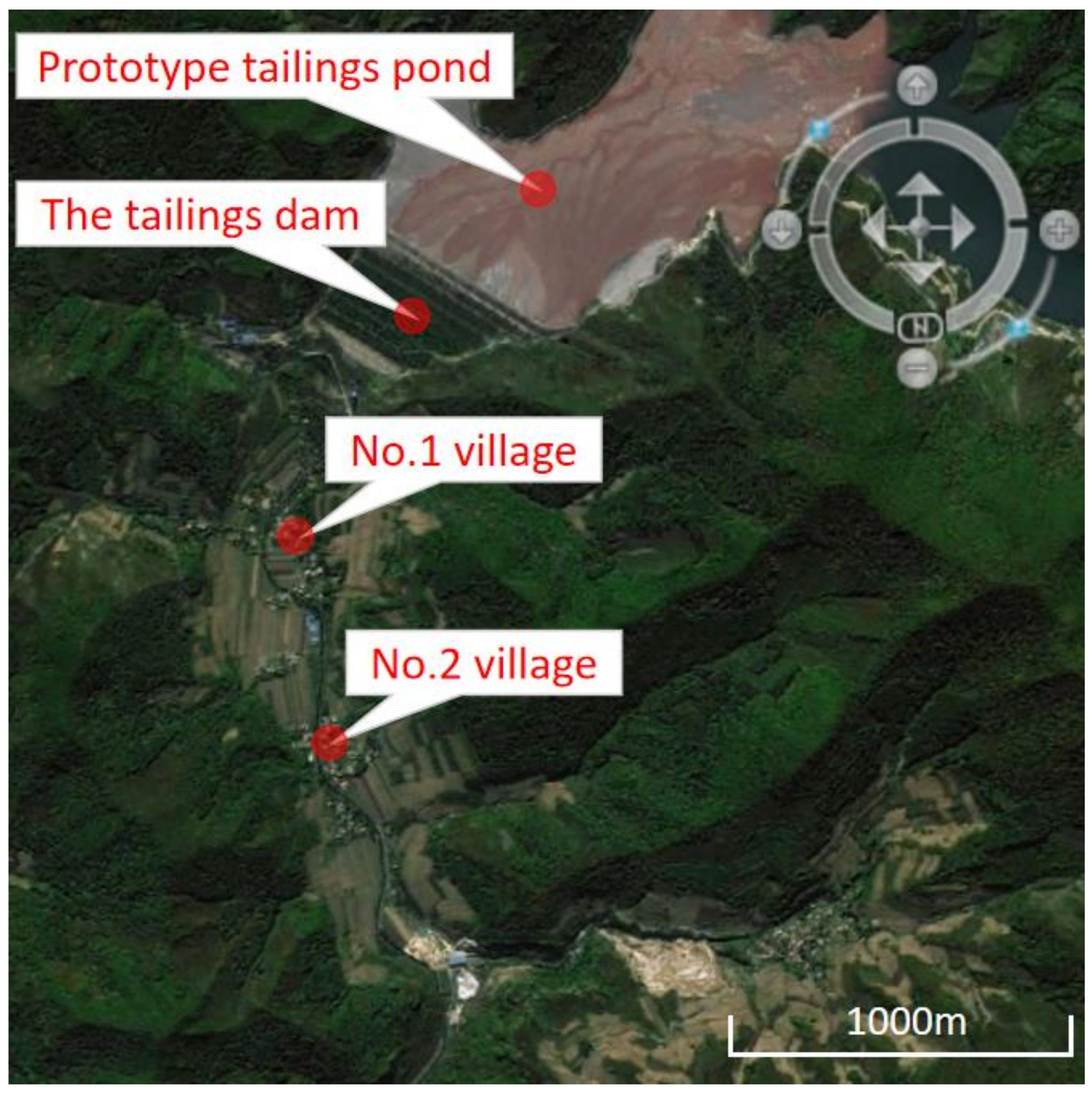
The original tailings pond is surrounded by mountains to the south, west and north, with two ditches at the end of the pond. The overall Y-shaped ditch opens to the north and east, which section is U-shaped, sloping from south west to north east. The elevation of the bottom of the ditch varies from 240 to 320 m, the elevation of the top of the mountain varies from 490 to 800 m, the maximum height difference is 400 m, the average slope of the longitudinal slope of the bottom of the ditch is about 3.28%, and the topography undulates minimally; this is a typical valley-type tailings pond. The initial dam bottom elevation is 240 m, the dam top elevation is 276 m, the dam height is 36 m; the initial dam upstream slope ratio is 1:1.85, and the downstream slope ratio is 1:1.7. The tailing pond sub-dam is of an “upstream type”, the dam top elevation is 380 m, the sub-dam outer slope ratio is 1:4, and the sub-dam road width is 8 m. The overall slope ratio of the accumulation dam is about 1:5; the total dam height of the tailing dam is 140 m with a total storage capacity of 260 million m3, and the tailing pond is classified as second class according to the Code for the Design of Tailings Facilities (GB 50863-2013). Village No. 1, with a population of 400 people, is 600 m downstream of the tailings pond, and village No. 2 is less than 1 km away. Due to the presence of important towns and industrial and mining enterprises downstream of the tailings dam, the grade of the prototype tailings pond is increased to first class, as shown in Figure 1.
3. Results Dam Failure Physical Model Test
3.1. Test Model
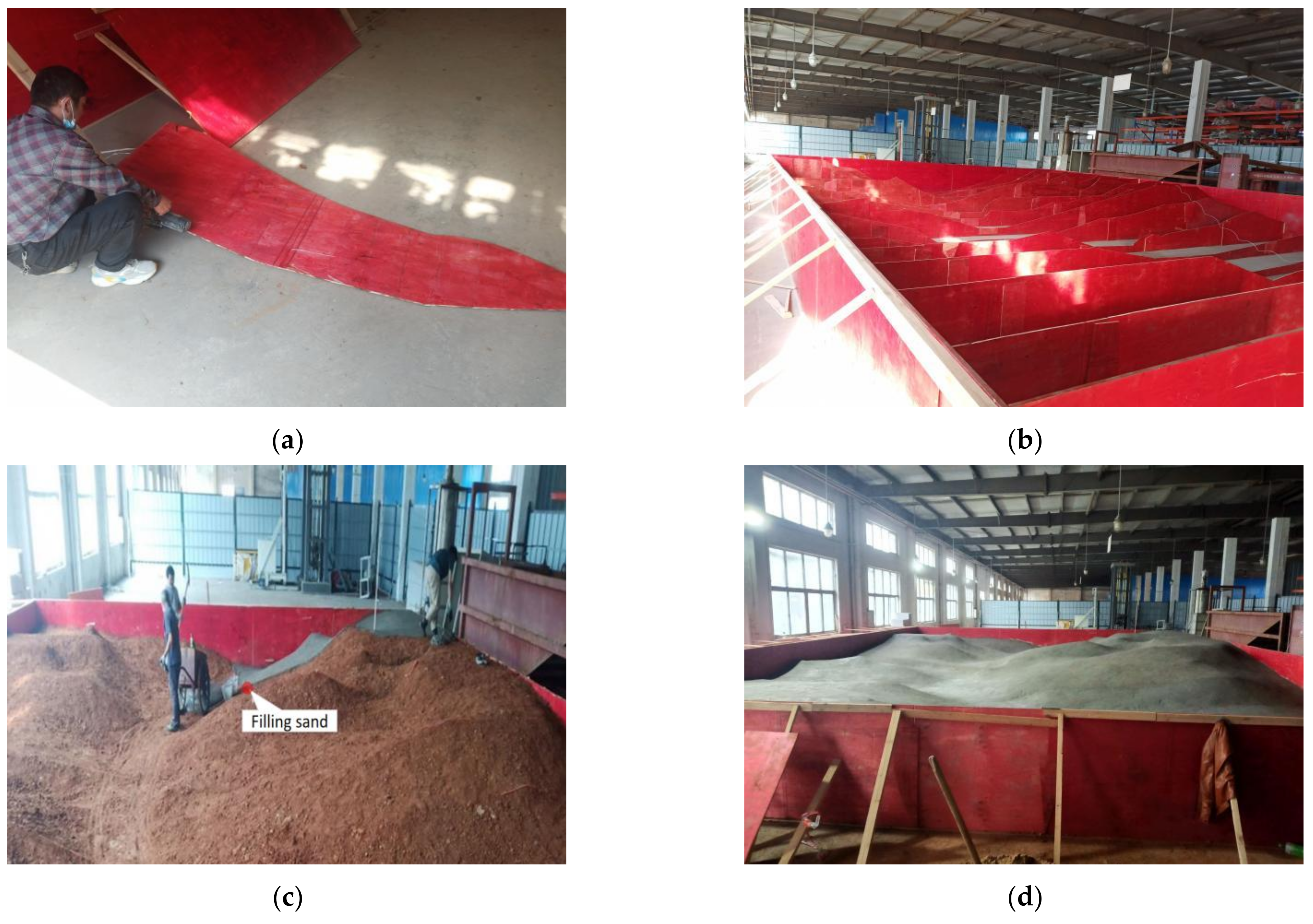
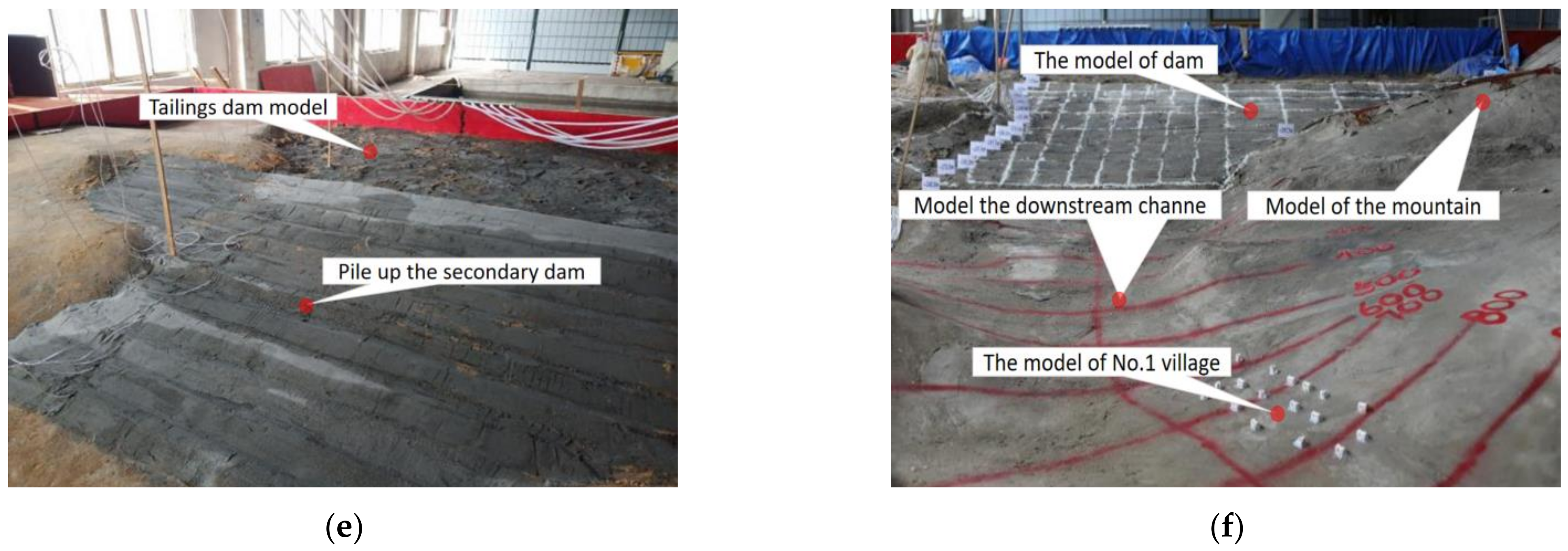
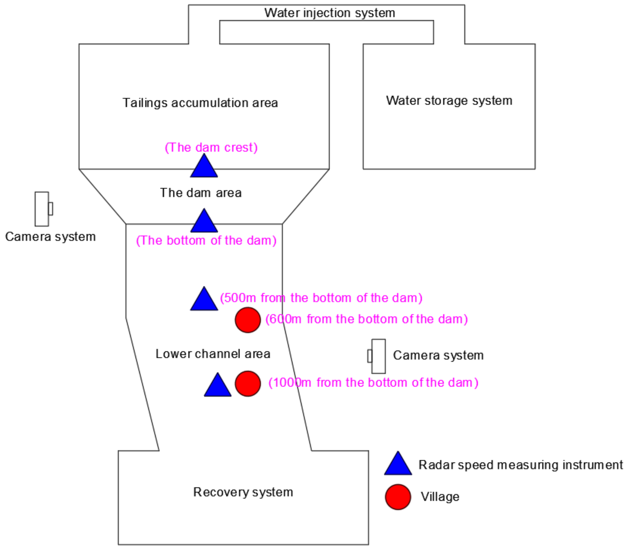
In the study of many mechanical problems, direct tests on the entity are costly and limited, and can only be applied to some specific situations; they also do not have universal significance, as it is difficult to use them to reveal the essence of the phenomenon and the general relationship between the quantities. Therefore, many problems are not suitably addressed via direct testing on the entity; similar model tests can replicate the huge scale of the entity, save money, control the parameters and achieve good targeting, prevent the influence of external environmental factors, have easily changeable test parameters for comparison tests, and yield accurate data. Therefore, the similarity of the model plays a decisive role in the test results. In the model-making process, the physical and mechanical properties, accumulation height and accumulation process of the sand, the slope, height and structural characteristics of the model dam, the slope, width and roughness of the downstream trench, the location of the village, the topographic relief and other influencing factors should be similar to the real conditions. Since the process of tailings pond breaching is extremely complex, there are many relevant factors and incompatibility is inevitable. This experiment aims to simulate the process of tailings pond breaching when flooding occurs, explore the evolution of the breaching law, and predict the impact range after breaching. Therefore, for our experimental purpose, the model’s general factors can be relaxed and we need only focus on the similarity of the accumulation effect [26]. For this test, the similarity of water flow hostage sand, the similarity of tailing sand settlement, and the similarity of tailing sand initiation should be satisfied, relative to the model scale λ. The similarity relationships between the other main physical quantities of the model are shown in Table 1. The model simulates the area of 3000 m × 2200 m of the prototype, according to the scale of 1:200; the height of the model tank is set to 1.2 m, and length × width is 15 m × 11 m. The initial dam of the prototype tailings pond is built using a permeable rock dam with a backfilter layer on the upstream slope, with a height of 36 m; above the initial dam, the upstream-type pile construction method is used, with the natural alluvial release of ore scattered on each level of the sub-dam in turn. The dam was built with bulldozers, with 12 levels of sub-dams at elevations of 283.30 m, 291.00 m, 297.66 m, 306.00 m, 313.50 m, 321.4 m, 331 m, 340 m, 349 m, 360 m, 370 m and 380 m. The slope ratio of the outer slope of the sub-dam is 1:4, the width of the roadway between the sub-dams is 8 m, and the overall slope ratio of the accumulation dam is about 1:5; the overall maximum dam height is 140 m. According to the ratio of 1:200, the initial dam height of the test model is 18 cm, and gravel was mainly used as the accumulation material. The ore was placed and compacted on the initial dam of the model. Each sub-dam was constructed in turn, and the overall maximum height of the model dam was 70 cm. the production process is shown in Figure 2. The test device consists of water storage system, water injection system, tailing accumulation area, dam body area, downstream river area, radar velocity measurement system, high-speed photography system, and recovery system, as shown in Figure 3.
3.2. Test Materials
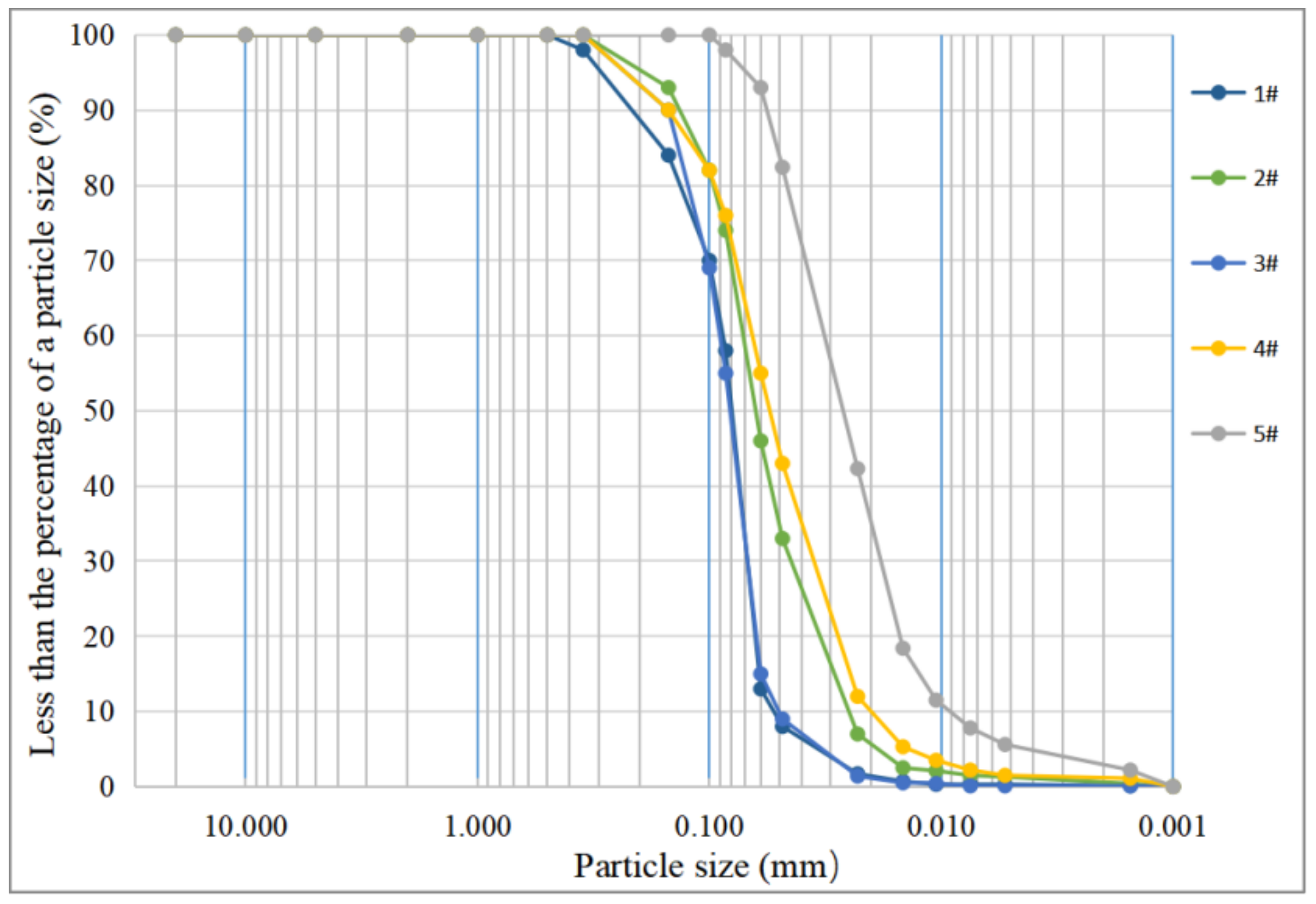
The model sand for this test was taken from the prototype tailing pond, and according to the geotechnical test methods and standards and protocols [27], the particle composition analysis and physical and mechanical property tests were conducted on the tailing sand. The physical and mechanical property parameters of the tailing sand were obtained as shown in Table 2, and the grain size gradation curves of the five groups of tailing sand are shown in Figure 4. The median particle size d50 of tailing sand is 0.0682 mm, mainly concentrated between 0.005 and approx. 0.075 mm, and the gradation inhomogeneity coefficient Cu is 2.76, which indicates poorly graded, powdered tailing sand.
3.3. Dam Failure Process
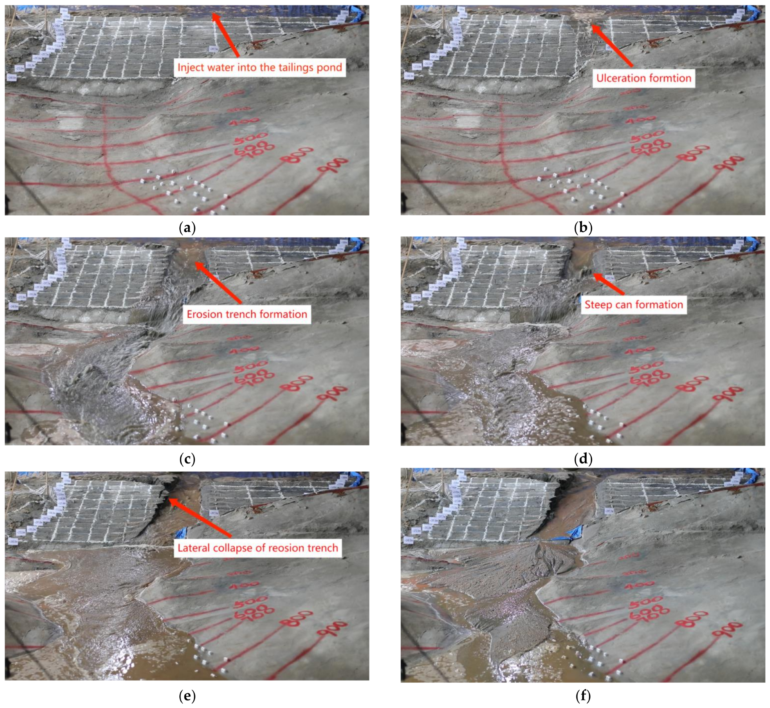
This test simulates the process of dam failure and the post-failure effects of the prototype tailings reservoir in the event of a maximum flood of 2000, due to the failure of the tailings reservoir drainage facilities to discharge flood water properly. The total amount of water injected into the test was 1.64 m3, according to the conversion of similar relationships. The amount of water injected was controlled through the water storage system. At the beginning of the test, water was supplied to the model reservoir through the water injection system, and the water level in the reservoir rose slowly, as shown in Figure 5a. When the water level spread over the top of the dam, the dam began to breach, and the change process from this point can be roughly divided into:
- With the slow rise of the water level in the reservoir, a small breach began to appear at the weak part of the dam top under the effect of water infiltration, as shown in Figure 5b;
- The water in the reservoir flowed from the breach to the bottom of the dam, and under the action of water erosion, the tail sand was carried away from the outer slope of the dam, forming an erosion trench, as shown in Figure 5c;
- With the development of the erosion trench, the discharged tail sand gradually transformed from the initial single movement to a group movement, and the tail sand in the erosion trench at the bottom of the dam first started to slip, forming a critical surface after slipping, and then forming a multi-level small steep bump in the lower part of the erosion trench. Subsequently, the multi-level steep cans gradually fused into one large steep can, which continuously expanded upstream until extending into the reservoir. During the migration process, a large amount of tail sand was carried away from the dam, and the depth of the erosion trench further increased, as shown in Figure 5d;
- While the steep moved upwards, the flood erosion rate increased, and when the dam body on both sides of the erosion trench was completely saturated, cracks appeared. When the bond force is weaker than gravity, the dam body collapses along the cracks into the trench, and the width of the erosion trench increases at a faster rate, as shown in Figure 5e;
- When the amount of flood water in the reservoir gradually decreased, the rate of increase in the width and depth of the erosion trench slowed down. When the flood water in the reservoir was fully discharged, the erosion trench stopped developing and the dam tended to a stable state, as shown in Figure 5f.
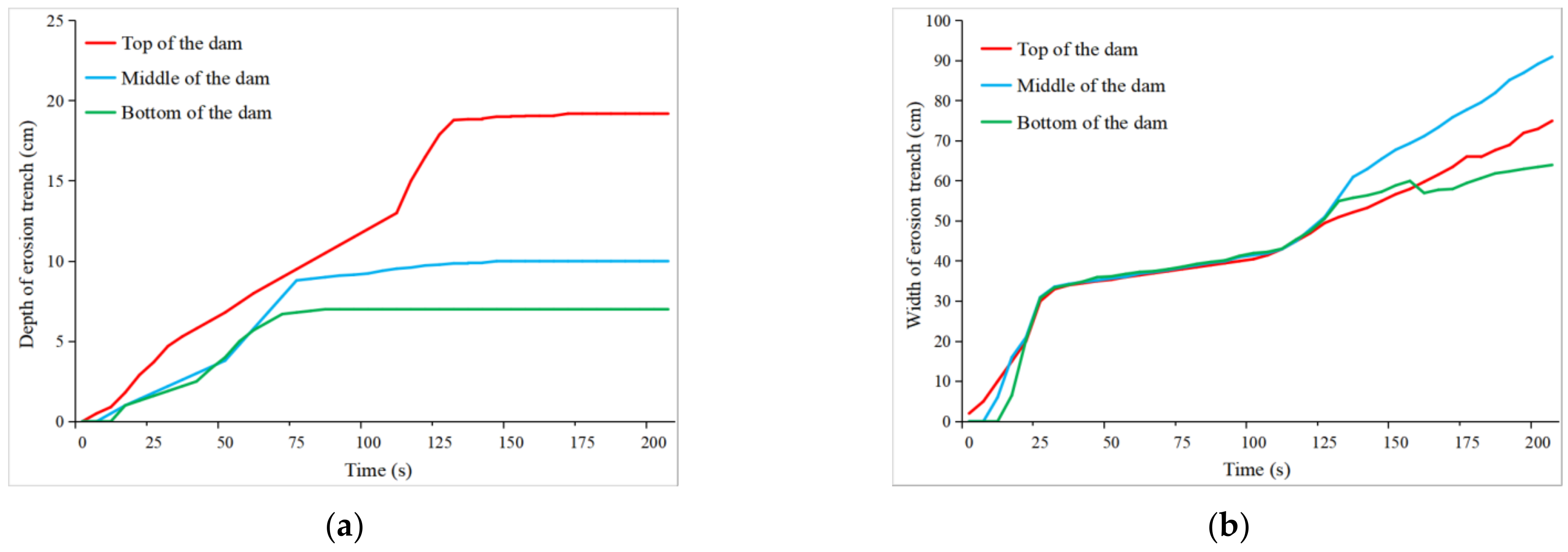
It can be seen from the dam breaching process that the breaching pattern evolves continuously with time during the breaching process, and the changes in breaching at the top, middle and bottom of the dam with time can be measured during the test. After the formation of the breach at the top of the dam, the water flowed downwards sharply, and the width and depth of the breach at the top, middle and bottom of the dam increased rapidly one after another. When a steep can is formed downstream of the breach, the depth of the breach at the bottom of the dam further increases. During the movement of the steep can upwards to the top of the dam, the depth of the breach in the middle and top of the dam increases with corresponding speed, as shown in Figure 6a, while the width increases relatively slowly, so it can be seen that the change in the shape of the breach at this stage mainly develops vertically. At the same time, the dam body on both sides was completely saturated while the breach was undercutting, and cracks and collapses occurred in the dam body. It can be seen that after the steep can moved up to the top of the dam, the width of the breach increased at a faster rate, as shown in Figure 6b, while the depth of the breach increased at a lower rate.
It can be observed from the dam-break process that the breach evolves continuously when the water volume in the reservoir is sufficient. The rate of evolution is related to the size of the water volume in the overflow section in the breach; the higher the water flow, the faster the evolution rate, and vice versa. It can be seen that the reservoir water storage capacity determines the final form of the breach’s evolution. In the operation of tailings ponds, the monitoring of the reservoir water level and the infiltration line in the tailings dam, as well as the management of flood control and other facilities, should be strengthened.
3.4. Evolution of Dam-Break Full-Field Velocity
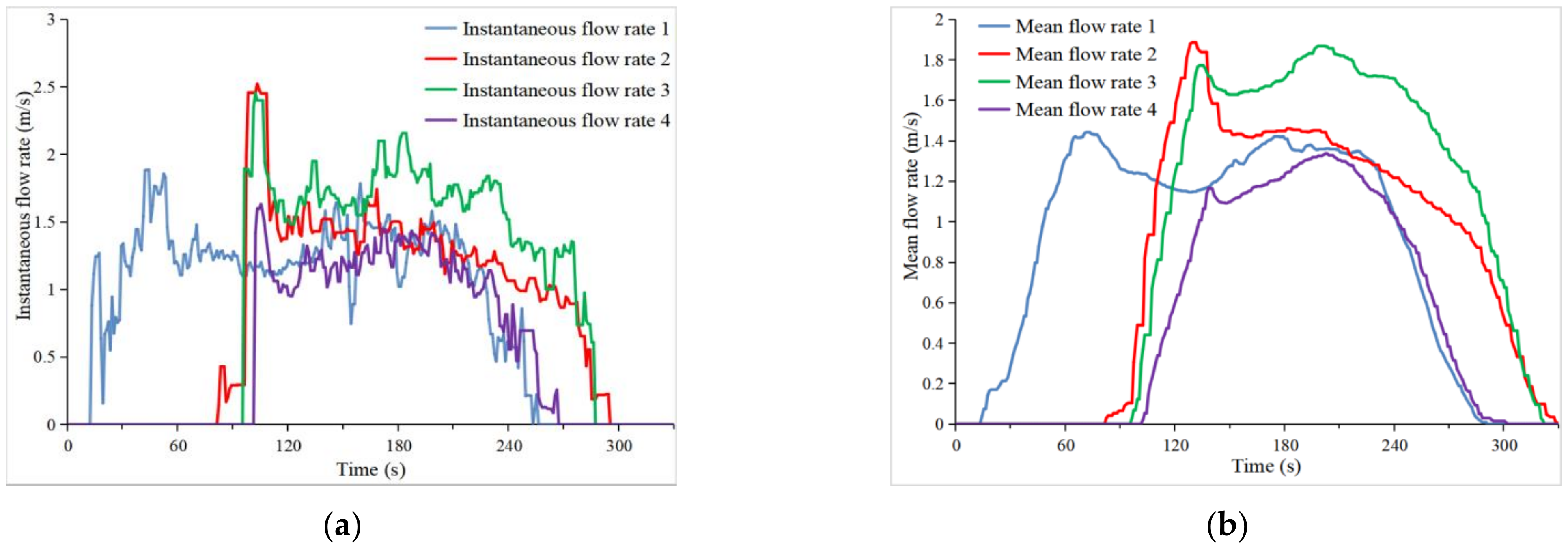
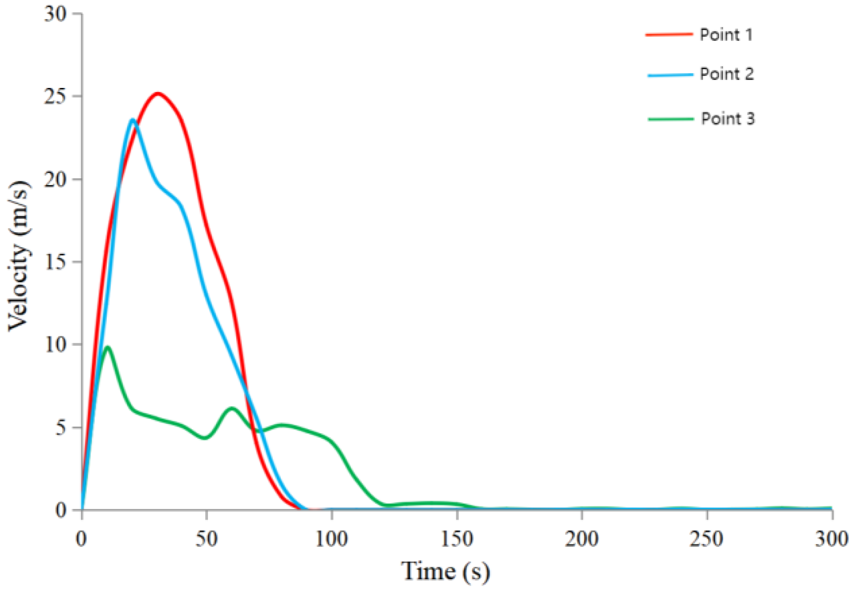
This test used four radar velocimeters to monitor the flow velocity in four areas during the dam breach: the top of the dam, the bottom of the initial dam, 500 m downstream of the initial dam and 1 km downstream of the initial dam, and the deployment locations are shown in Figure 3. The measurement results of the variations in velocity with time during the dam break are shown in Figure 7 below.
By comparing and analyzing the flow velocity changes of the four measurement points, we see a pattern of rapid increase > relatively stable > slow decrease. The maximum flow velocity shows a pattern of shifting from measurement point two to measurement point three. This is due to the characteristics of the high potential energy and large volume of flood water in the reservoir, so when the breach occurs at the top of the dam, the flood water comes down rapidly and the whole field of flood water advances rapidly, reaching the peak flow velocity in a short time. The flow velocity in the area of measurement point two is the largest, where the maximum average flow velocity is 26.68 m/s; this is followed by measurement point three, measurement point one and measurement point four. After that, as the water level in the reservoir is still high, the flood water recharge is sufficient, so it maintains a relatively stable speed for a period of time. The flow velocity of measurement point two decreases after reaching the peak at this stage, while measurement point three does not decrease—the flow velocity in this area is the largest, at 26.43 m/s. This is followed by measurement point two, measurement point one and measurement point four. This indicates that the flow velocity at the bottom of the initial dam is the highest at the beginning of the dam-breaching process, and the flow velocity 500 m downstream from the initial dam is the highest at the middle of the dam breaching process (the most relatively stable stage of the downstream flood). Since the impact of the tailing sand on the downstream area is proportional to the square of the maximum moving velocity, the impact of the flood water at the bottom of the initial dam is the largest during the development of the dam failure process, and it then shifts to the area 500 m downstream. For a specific project, prevention and control measures can be formulated by taking into account the evolution process of post-break flood flow velocity and the downstream facilities of the tailings pond, etc., in order to minimize the degree of post-break damage.
3.5. Post-Dam Failure Impacts
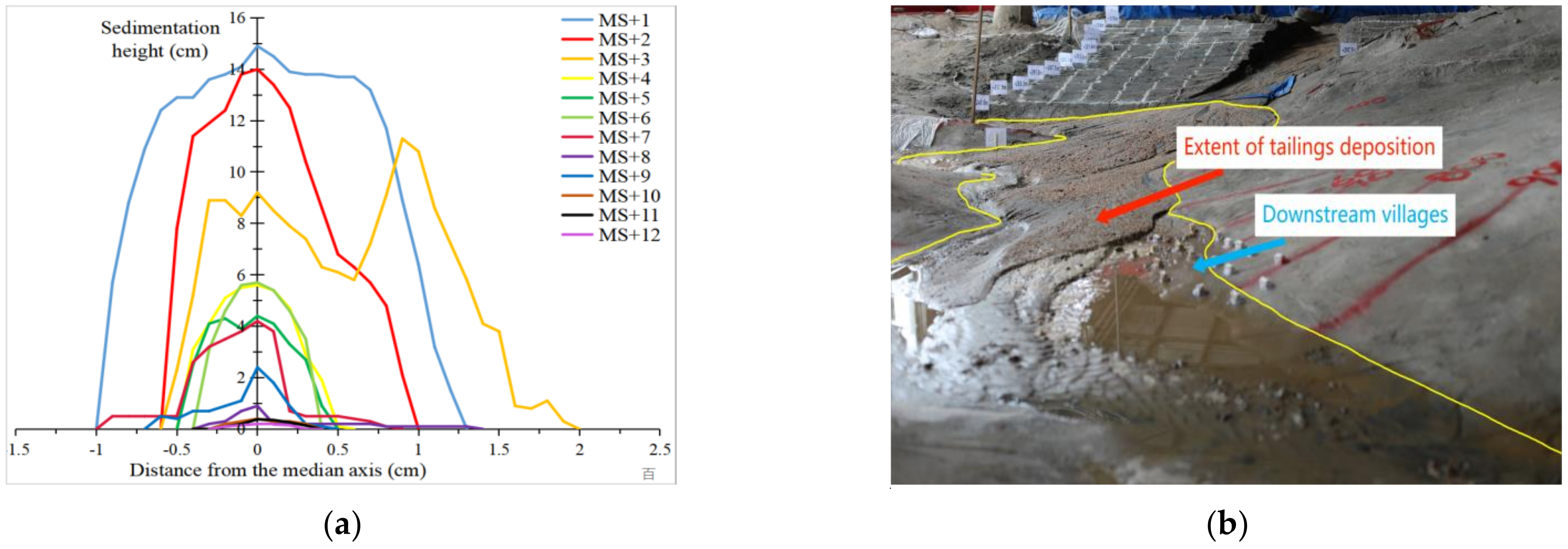
In order to more accurately determine the evolution of the tailing sand accumulation depth and the degree of impact on the downstream, we took the bottom of the initial dam as the starting point and set up a measurement section every 100 m from the prototype, which points were numbered MS+1 to MS+12. After the dam-breaching process, the accumulation width and depth of the tailing sand were measured in each section. The results are shown in Figure 8a. From the physical model test, it can be inferred that most of the houses in village 1 will be flooded by the tailing sand 600 m away from the prototype tailing pond breach, and the houses on higher terrain will not be flooded by the tailing sand but will be flooded with water. Village 2, which is within 1 km, will be flooded, as shown in Figure 8b. The greatest distance of tailing sand siltation is about 1.19 km from the initial dam, and the maximum siltation depth is 29 m. The volume of flood water discharged in the breach is much larger than the volume of tailing sand carried by it, and the downstream terrain of the tailing pond is of a gully type, so the flood inundation range is much larger than the siltation range of tailing sand, which former is 4.76 × 10⁵ m2. The larger the size of the tailing sand, the larger the elevation of the foundation in the same section, the smaller the accumulation depth, and the larger the particle size; the maximum accumulation depth of the tailing sand is 14.5 cm.
4. Numerical Simulation
4.1. Numerical Model
In order to more accurately study the tailings pond breaching process and post-breaching effects, this paper uses two numerical softwares with different principles to simulate the tailings pond breaching process and compare and analyze the results regarding the post-breaching effects, with a view to comparing multiple methods and then reasonably determining the evolutionary law and post-breaching effects. Massflow is a ground surface simulation program based on the depth integral and MacCormack-TVD finite difference method. It can simulate the dynamics process of landslides, debris flows, dam failures and other hazards by considering complex terrain and landscapes. Chaojun Ouyang et al. used Massflow-2D to model the 2000 Nora mudflow in the Italian Alps, and verified its accuracy by comparing simulation predictions with field observations [28]; Alexander J. Horton et al. applied the Massflow model to simulate the risk of mudflow after the Wenchuan earthquake in China [29]; Wang Dongpo et al. summarized the relationship between vegetation cover and post-fault inundation area, water depth and flow velocity based on the Massflow model in Jiuzhaigou, Sichuan, China [30]. Smoothed Particle Hydrodynamics (SPH) is a meshless method that has developed gradually in the last 60 years. The basic principle of this method is to decompose a continuous fluid or solid into groups of interacting masses, and finally sum up the mechanical behavior of the whole system by determining the mechanical behavior on each mass group separately. It can be seen that SPH analysis is very effective when applied to problems involving extreme deformation, and is especially suitable for solving dynamic large deformation problems such as high-speed collisions and fluid motion. Huang et al. used SPH to analyze the migration law of landslide and debris flow hazards in relation to the Wenchuan earthquake [31]; Vacondio et al. applied SPH to simulate the law of water flow caused by landslides in reservoirs, and the simulation results effectively reproduced key parameters such as the maximum climbing distance and height of water flow [32]; Rodrigue-Paz et al. proposed a modified friction boundary conditions method, and introduced the improved instantonal equations into the SPH method to simulate mudflow hazards based on the CSPH (Corrected Smooth Particle Hydrodynamics) theory—the numerical solution matched the experimentally obtained test results with good accuracy [33]; Dai et al. established a coupled SPH model to simulate mountain mudflow–structure interactions [34]; V. Roubtsova et al. performed a three-dimensional simulation of the Vaiont dam disaster that occurred in northern Italy in 1963 to verify the applicability of the SPH technique to problems in free surface flow [35]; Mahesh Prakash used the SPH method to simulate the 1928 Francis dam failure and studied the distance and depth of post-failure flood impact [36]. Andreia Moreira et al. applied the SPH method to predict the flow characteristics of the spillways and dissipaters of the Crestuma and Caniçada dams in Portugal [37].
Therefore, the Voellmy model and the Herschel–Bulkley model can be used to numerically simulate the tailings pond breach process using Massflow and SPH, respectively, as shown in Figure 9. The model is 2800 m long and 2000 m wide. The shape of the breach in the model is set with reference to the slip surface shape (range and depth), obtained from the dam stability analysis, and the breach shape (width) obtained from the physical model test, while the breach range is set slightly larger in order to model the most unfavorable situation. Based on the natural density of the tailing sand in the survey report and the residual strength parameters obtained from the ring shear test, the density parameter of the Voellmy model can be set to 1950 kg/m3, the friction coefficient is set to 0.26, and the Herschel–Bulkley model has five basic parameters: η0 is the shear viscosity at low shear rate, τ0 is the yield shear stress, k is the consistency index, n is the flow characteristics index, and C0 is the temperature. These five basic parameters and the state parameters (using the linear three-parameter USUP equation of state) are usually determined with specific reference to the tailings sand parameters commonly used in the literature [38,39,40], and in conjunction with the field tailings sand conditions. The breaching of the dam occurred in a relatively short period of time; the temperature change can be ignored, and so the effect of temperature was not considered. A sensitivity analysis was performed on the relevant parameters, and the results show that the friction coefficient is the main parameter affecting the flow range and accumulation characteristics. The residual strength parameter obtained from the ring shear test, i.e., 0.26, was used for this calculation, and the other parameters are shown in Table 1, Table 2 and Table 3.
4.2. Analysis of Massflow Calculation Results
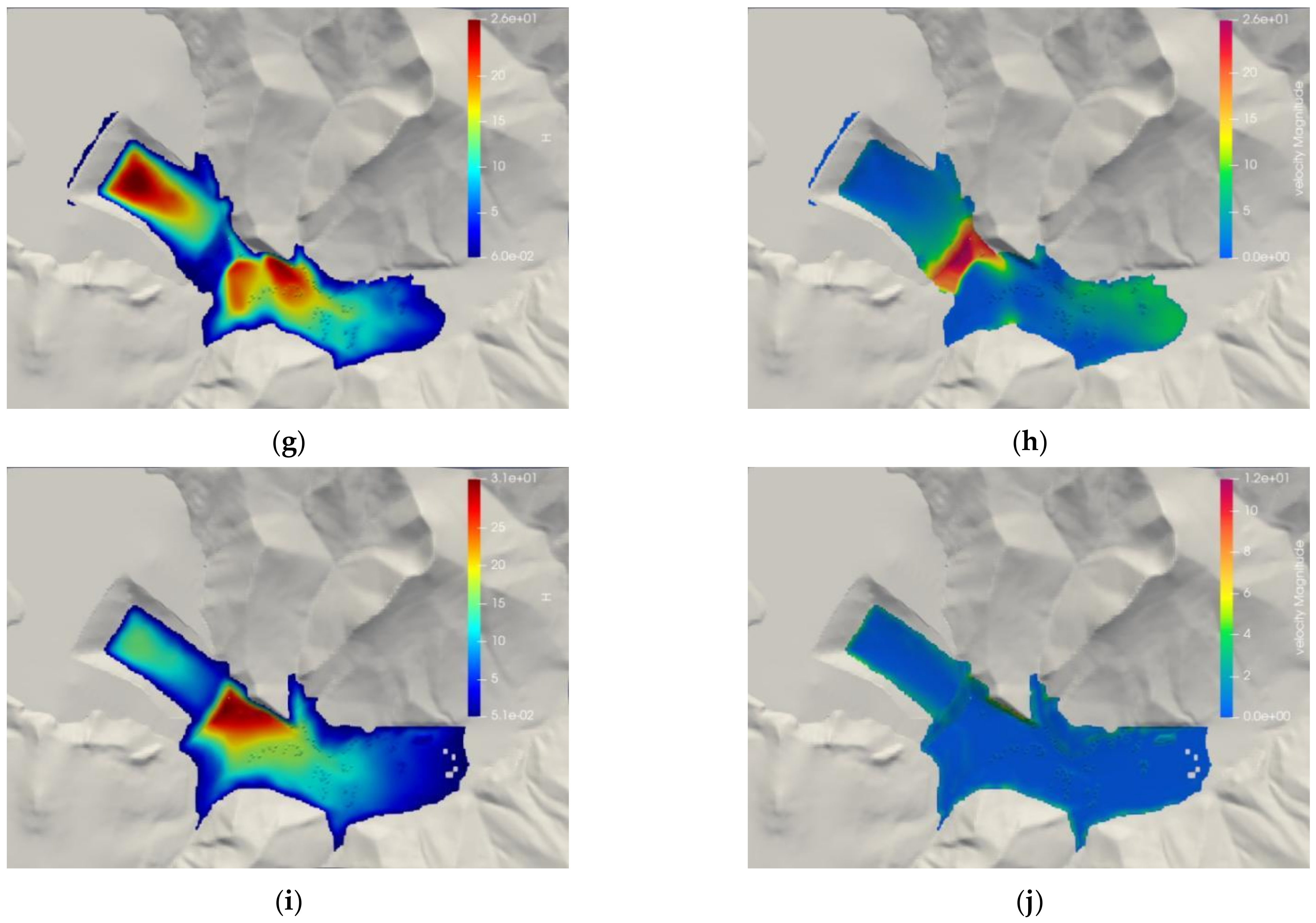
The process of dam-break tail sand flowing downstream can be modeled through numerical simulation, as shown in Figure 10:
- At 20 s, the maximum accumulation height of the tail sand was about 48.8 m, mainly located in the reservoir area, and part of the sand flow advanced to 350 m downstream. The overall speed of the sand flow ahead of the breach was fast—the maximum was 30.2 m/s, and the direction was northeast;
- At 40 s, the maximum accumulation height of the sand flow was about 33.6 m, located in the reservoir area, and the farthest reach of the sand flow was 670 m downstream. The overall speed of sand flow in front of the breach was still fast, with a maximum of 30.0 m/s, and the direction began to shift northward due to the influence of the mountain;
- At 60 s, the maximum accumulation height of the sand flow was about 31.5 m, mainly located in the reservoir area and 250 m in front of the right side of the dam, and the sand flow reached as far as 1060 m downstream. The maximum travel speed of the sand flow was 27.1 m/s, located directly in front of the breach, and the travel speed of the front edge of the sand flow was reduced by ground friction and the blocking effect of the right side of the mountain to about 16.0 m/s. The direction had turned due north at this point;
- At 80 s, the maximum accumulation height of the sand flow was about 26.2 m, mainly located in the reservoir area and 340 m in front of the left side of the dam, and the sand flow reached as far as 1290 m downstream. The maximum travel speed of sand flow was 25.7 m/s, and the travel speed of sand flow within 150 m of the breach exceeded 20.0 m/s. The travel speed of the front edge of the sand flow decreased to 7.0 m/s, while the flow speed in other areas decreased to 1.0 m/s or less;
- At 300 s, the sand flow movement basically stopped. The final evolution distance was about 1.43 km, the tail sand accumulation range reached 603,000 m2, and the whole was distributed in strips along the downstream gully, with part of the sand flow entering the gully on both sides. The buildings of the village within 1 km downstream of the dam body were completely submerged—only in the area where the accumulation height of the sand flow front edge was less than 3 m were a small number of village buildings partially submerged. The accumulation height along the evolution path was generally decreasing, and the maximum accumulation area was at the left side of the mountain in front of the dam, with a maximum accumulation height of about 31.5 m.
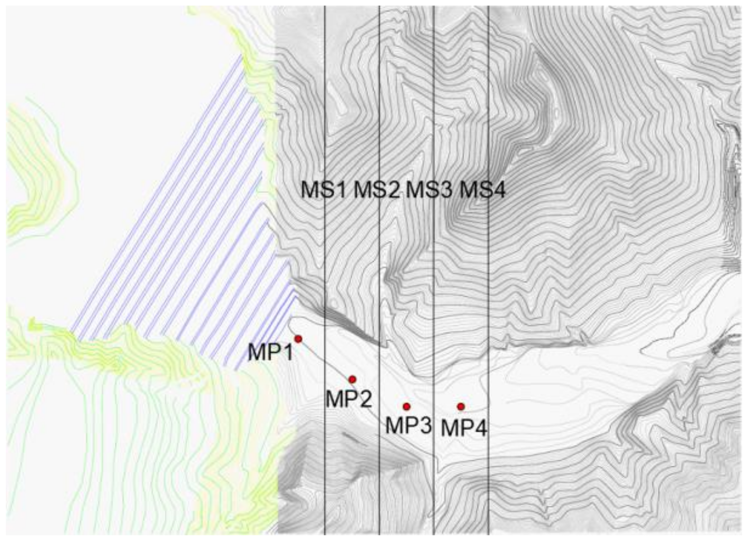
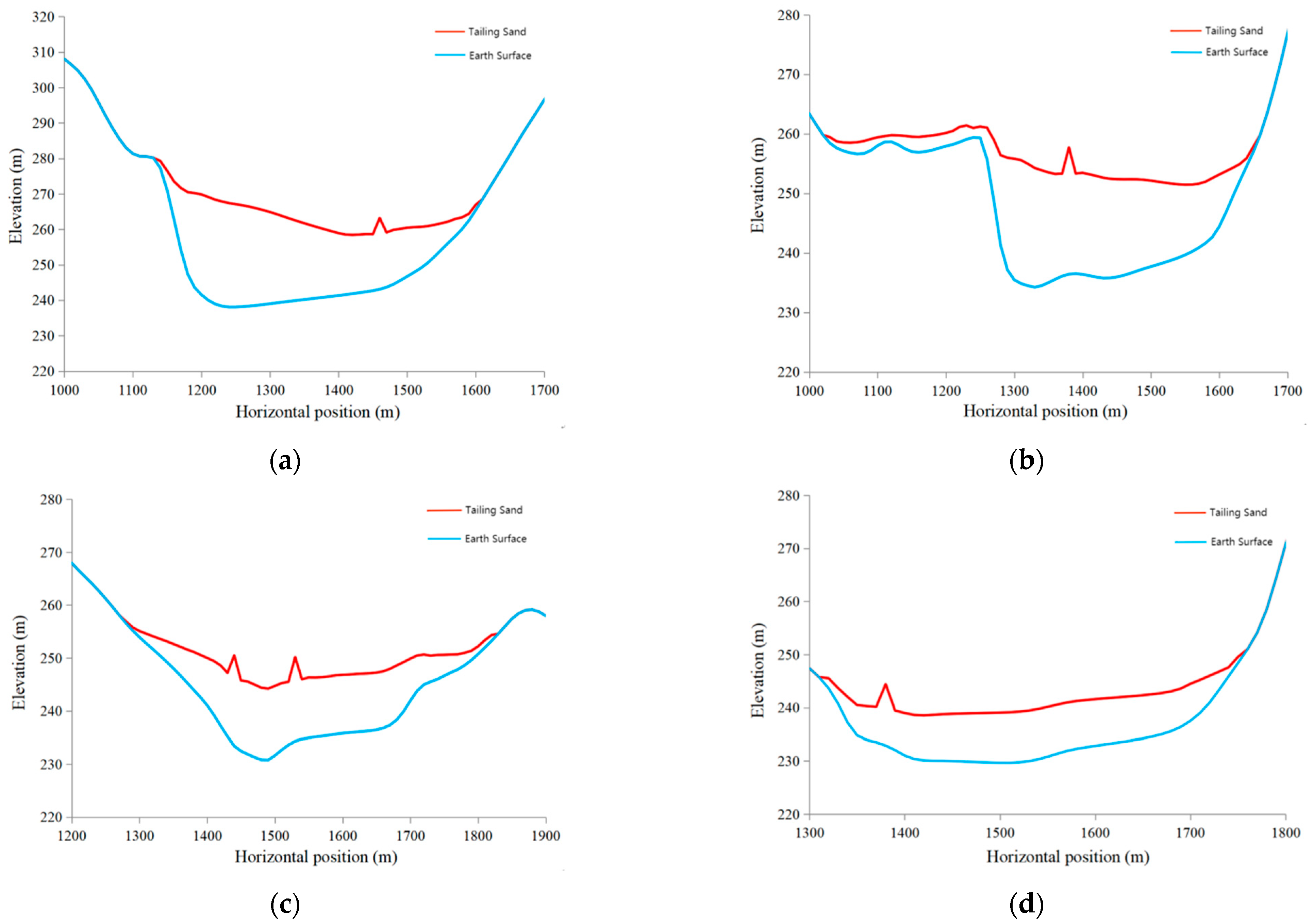
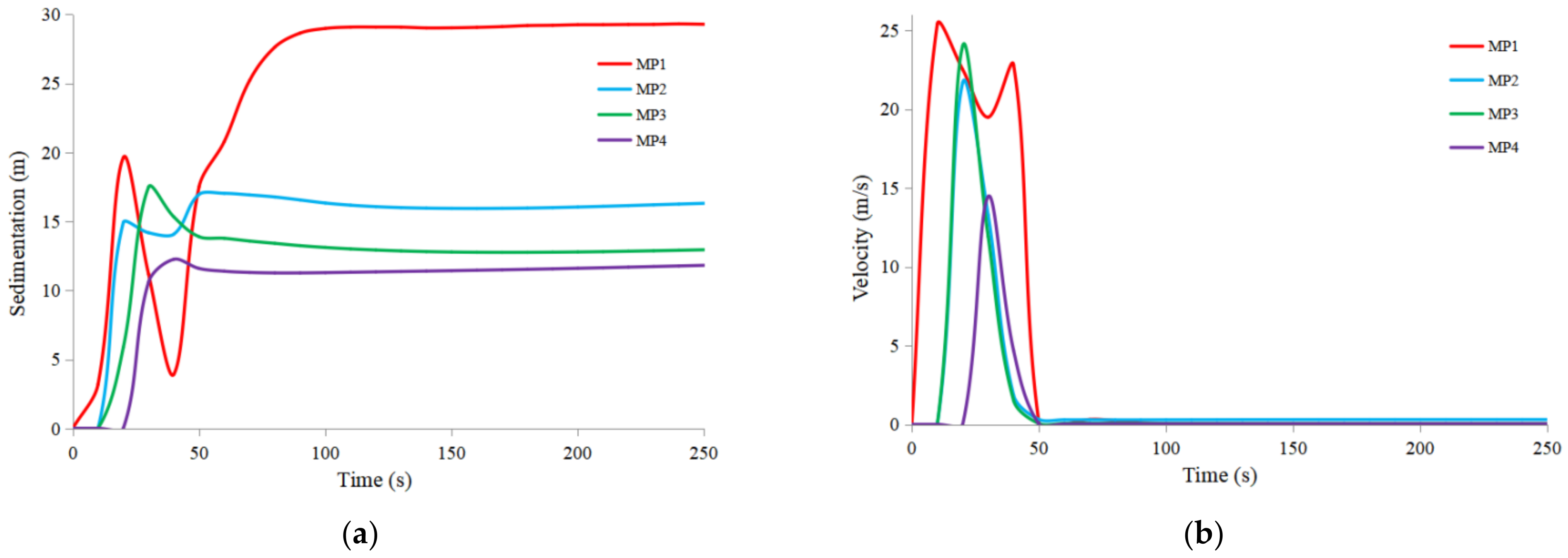
In order to derive a more intuitive picture of the spatial and temporal evolution of tailing sand accumulation, four monitoring sections (MS1~MS4) and four monitoring points (MP1~MP4) were set up downstream of the dam, the specific locations of which are shown in Figure 11. The tailing sand accumulation pattern at each monitoring section after the end of the dam break is shown in Figure 12, the change of tailing sand accumulation height at each monitoring point during the dam break is shown in Figure 13a, and the change of sand flow velocity at each monitoring point with time is shown in Figure 13b. It can be seen that:
- The tailing sand accumulation on the left side of sections MS1 and MS2 is significantly higher than on the right side, the accumulation at MS3 is low in the middle and high on both sides, and the accumulation on the right side of MS4 is higher than on the left side due to the sand flow being diverted by the mountain. The presence of village buildings will increase the accumulation height in the area;
- The tailing sand accumulates rapidly in the downstream channel after the breach. Before 50 s, a large amount of tailing sand is discharged per unit of time, the potential energy is large, the tailing sand accumulation distance is great, and the tailing sand accumulation height at each measurement point increases rapidly. After 50 s, a small amount of tailing sand is discharged within a unit of time, the potential energy is small, the tailing sand accumulation distance is small, and the tailing sand accumulation height at locations far from the initial dam no longer increases, while the accumulation height near to the dam body continues to increase. The tailing sand accumulation height curve at monitoring points near the dam is bimodal, and can be divided into four stages, i.e., sharp rise–significant decline–continuing to rise–gradually stabilizing, and the tailing sand accumulation height curve at monitoring points farther away from the dam is largely unimodal, and can be divided into three stages, i.e., sharp rise–small decline–gradually stabilizing;
- The change in the velocity curve at the monitoring points near the breach is more complicated—the sand flow is faster and the movement lasts longer. The velocity curve at other monitoring points essentially shows a steep rising and steep falling triangular shape—the sand flow velocity is reduced and the movement lasts for less time.
4.3. Analysis of SPH Calculation Results
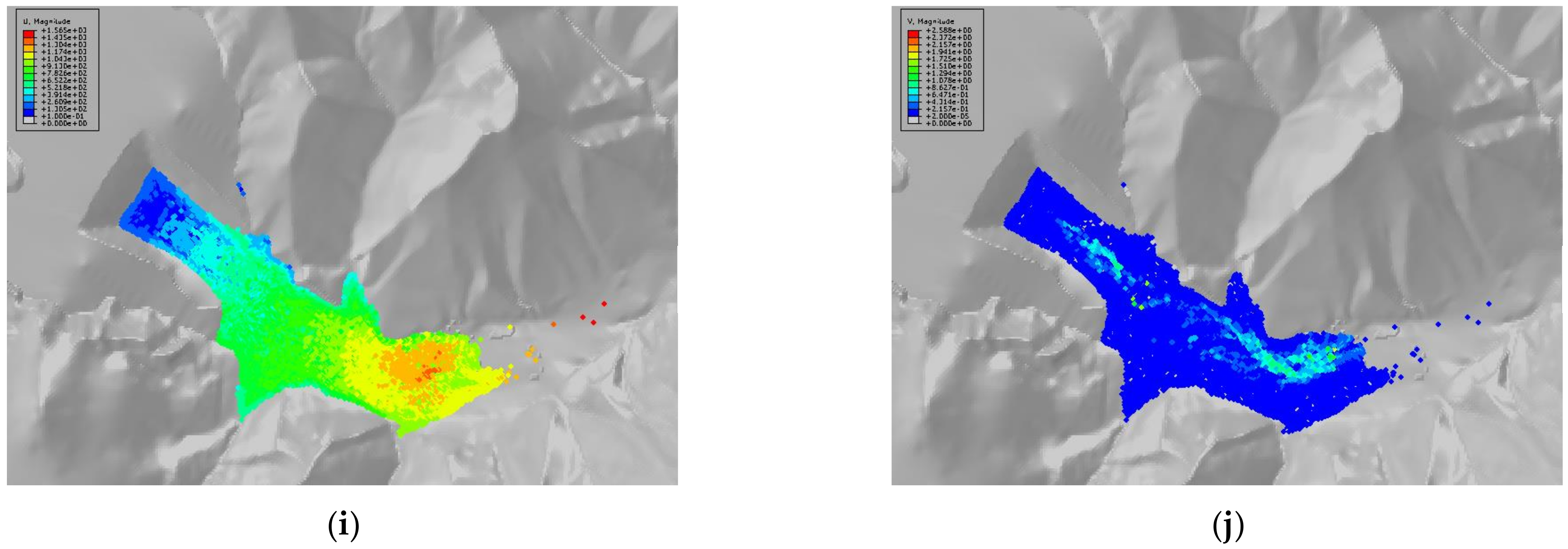
The SPH was applied to simulate dam failure in the prototype tailings pond, as shown in Figure 14.
- At 20 s, the maximum displacement of the breached tailing sand was about 320 m, and the tailing sand movement speed was fast, with a maximum of about 33.0 m/s;
- At 40 s, the maximum displacement of the breached tailing sand was about 820 m, and the sand flow movement speed was more evenly distributed, with a maximum of about 29.9 m/s;
- At 60 s, the maximum displacement of the breached tailing sand was about 1120 m, and the sand flow front and the tailing sand movement speed in front of the breached opening were at their maximum;
- At 80 s, the maximum displacement of the tail sand of the breached dam was about 1250 m, and the maximum velocity of the tail sand movement was about 18.0 m/s in front of the breached mouth and the front edge of the sand flow, while the velocity of the tail sand movement in other areas had dropped to less than 6.0 m/s;
- At 300 s, the maximum displacement of the tail sand of the breached dam was about 1350 m, and the tail sand movement had basically stopped. The sand accumulated in strips along the gully, with some of the tail sand flowing downstream. At both sides of the ditch, the accumulation range reached 527,000 m2, and village buildings within this range were completely submerged.
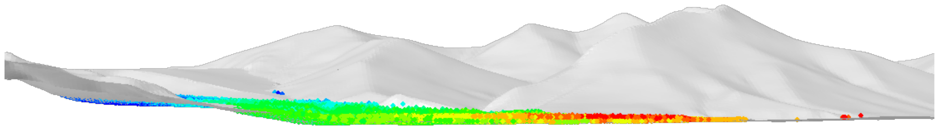
Since the SPH method cannot directly give the tailing sand accumulation height, the accumulation state of the downstream tailing sand can only be generally observed here through the profile of the post-failure river channel, as shown in Figure 15. The downstream river channel shows a pattern whereby at points further away from the tailings dam, the depth of tailings accumulation is shallower.
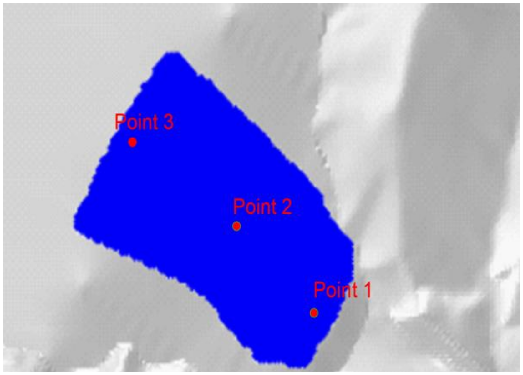
In order to analyze the evolution law of the tailing sand movement during the dam-break process, several monitoring points were selected on the breached tailing sand body (Figure 16), and the velocity–time curves of tailing sand movement at each monitoring point are shown in Figure 17. It can be seen that the velocity of the tailing sand can be divided into two parts during the breaching process: In the front part of the breached body under the action of high gravitational potential energy in the tailing sand, the velocity of the tailing sand increases sharply and then decreases sharply, and the velocity–time curve is basically a triangle with a steep rise and a steep fall. The rear part only shows a small degree of tailing sand discharge; the overall potential energy is small, and the flow velocity of the tailing sand discharge is slow and stabilizes after a long time.
5. Results and Discussion
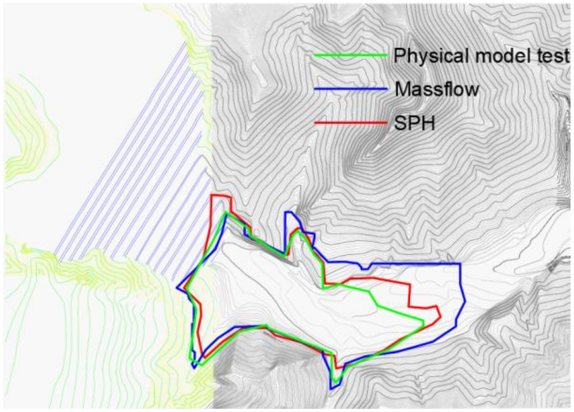
The two numerical simulation results are compared with the physical model test results (see Table 4 and Figure 18). The two numerical simulations have different principles (SPH is a particle method based on continuous medium, while Massflow is a finite difference method), and the ontological material parameters used by the two are also different; therefore, there is a gap between their simulation results. Compared with Massflow, the evolution distance and accumulation range of tailing sand obtained by SPH simulation are small, and the difference in tailing sand accumulation range is large. This is due to the fact that SPH relatively realistically considers the fluid-like shear viscous behavior of the tailing sand, so the greatest evolution distance and accumulation range of the tailing sand obtained from this simulation are smaller than those from Massflow. Comparing the results of the two methods, numerical simulation and the physical simulation test, we see that the difference is not significant, which confirms the accuracy of the physical model test and the feasibility of these two numerical simulation methods. However, there are also differences, as shown below:
- There is a lag in the physical model test when the maximum flow velocity of the discharged tailings sand appears during the dam breach process, reaching the peak flow velocity of 120 s after the breach appears at the top of the dam, after which it remains relatively stable for a period of time and then starts to decrease rapidly. On the other hand, the numerical simulation reaches the peak flow velocity of the discharged tailings sand at the beginning of the dam breach and then rapidly decreases to close to 0 m/s, creeping for a longer period of time before the end of the dam breach;
- The tailing sand flow velocity, evolution distance and depth obtained from the numerical simulation are large. This is because (i) the breach pattern in the numerical simulation is set with reference to the physical test, but in order to consider more unfavorable conditions, the breach is set larger and deeper, and the total volume of the breached tail sand is slightly higher, and further, (ii) the numerical simulation does not truly reflect the model test conditions and processes. In the test, rainfall continues to wash the breach, carrying the tail sand continuously downstream, and there is obvious mud–water stratification in the tail sand flow, while the numerical simulation is instantaneous. In the full-break mode, the potential energy of the tailing sand body is released instantaneously, while the tailing sand and water are completely mixed, and the flowability is good in all directions.
Thus, Massflow and SPH can be used to quickly and easily simulate and predict the impact range of the tailings pond after the breach, but if the purpose is to study the evolution of the tailings dam and the downstream tailings during the breach process, the physical model test can better reflect the real situation.
6. Risk Assessment and Recommendations
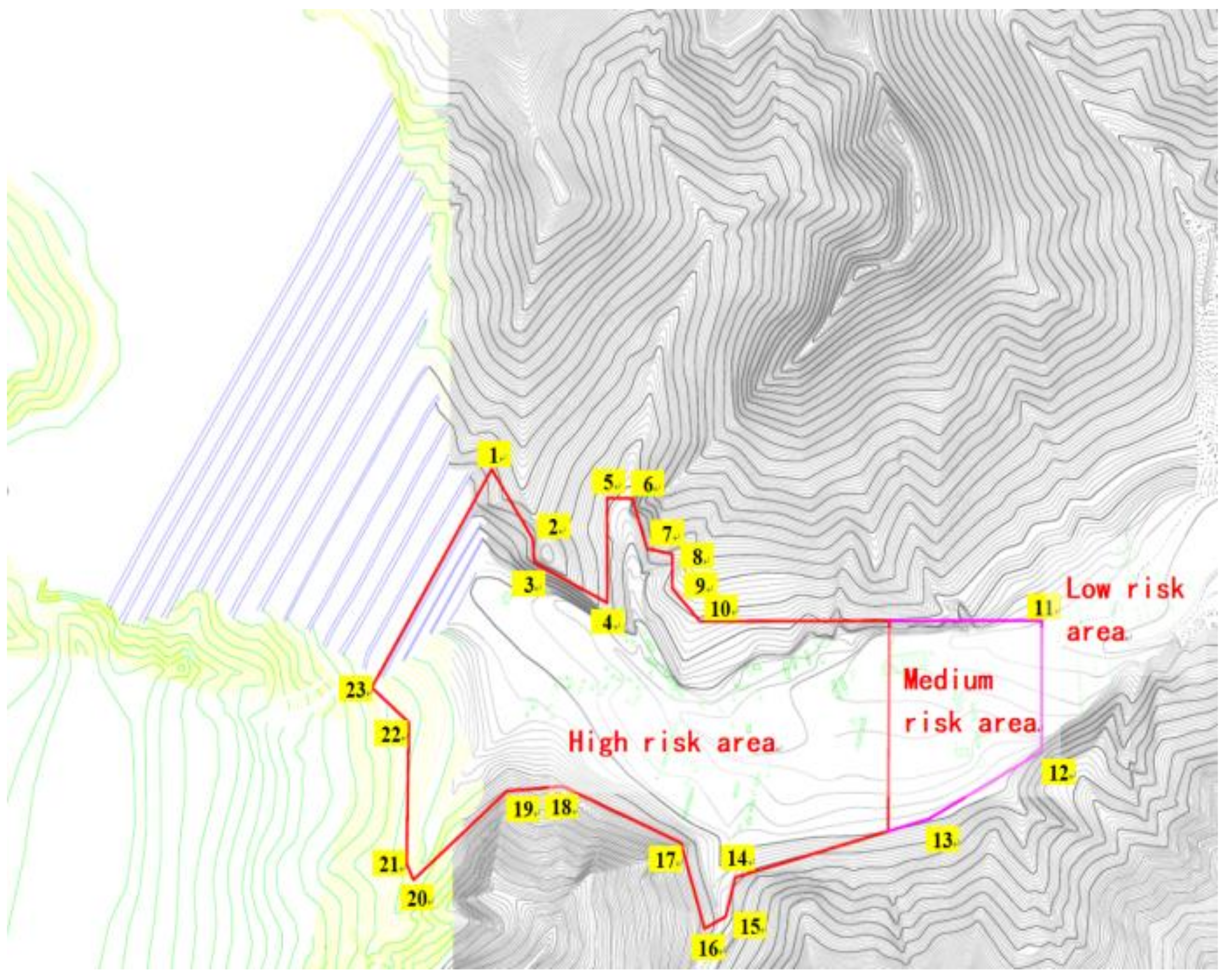
There are differences between the physical model test’s results and the numerical simulation, and the larger value should be used as a reference when carrying out engineering, prevention and control. After a comprehensive analysis, it can be determined that the maximum flow velocity of tailing sand occurs at the bottom of the initial dam, and the maximum flow velocity can reach 35.01 m/s. The final evolution distance of tailing sand after breaching can reach 1.43 km, the accumulation range can reach 60.30 m2, and the maximum accumulation depth can reach 31.50 m. Based on the maximum flow velocity and the accumulation depth of tailing sand, the river downstream of the tailing pond can be divided into risk areas. In this way, relocation measures can be formulated. In high-risk area, the flood flow velocity is fast—the maximum flow velocity is above 14.85 m/s—and the impact force is high, the accumulation height is over 6 m, and the destructiveness is strong. In the medium-risk area, most of the kinetic energy is consumed and the travel speed is greatly reduced, so the maximum flow velocity is below 14.85 m/s. The accumulation height is also reduced—the accumulation height is below 6 m, and the destructiveness is further reduced. In low-risk areas, the tailings accumulation area is outside the inhabited area. The low-risk area is outside the tailings accumulation area; this area includes a large amount of farmland, villages and industrial facilities. This area is not affected by the dam failure, and the warning and personnel evacuation times will be sufficient—see Figure 19.
7. Conclusions
This paper explores the evolutionary law of tailings pond breaching under flood breach conditions and the post-breaching effects, using indoor model tests and numerical simulations, as follows:
- During the breaching process, after the tailings dam forms an erosion trench, the lower part of the erosion trench is the first to slip, and after the formation of a steep can, the upper part of it causes slippage in the tailings, such that the erosion trench first develops vertically and then laterally. The final evolution of the breach is determined by the amount of water stored in the reservoir;
- When the top of the tailings dam is breached, the downstream tailings sand flow rate will quickly reach a peak value of 33.00 m/s in a short period of time, after which the downstream tailings sand flow rate reduces to a creeping state. After creeping for a long period of time, the front edge of the sand flow is the first to stop moving, while the trailing edge of the tailings sand accumulation depth continues moving until the end of the breach, at which point the tailings sand flow rate of the initial downstream dam bottom area is the largest. The impact force is the most significant factor use to form prevention and control measures;
- The discharged tailings eventually accumulate in the downstream channel, showing a pattern whereby at points further away from the initial dam, the accumulation depth will be smaller and the particle size will be larger, while the larger the elevation of the foundation in the same section, the smaller the accumulation depth and the larger the particle size. The maximum accumulation depth is 31.50 m, at which point the presence of shade will cause the local tailings accumulation depth to increase;
- There are small differences between the results of the numerical simulation and physical model tests, and the bias value should be used as the basis when carrying out engineering prevention and control measures. The final evolution distance of tailing sand after the collapse can reach 1.43 km, and the maximum accumulation depth can reach 31.50 m. Based on the flow velocity, downstream tailing sand accumulation distance and depth, the risk area of the river downstream of the tailing pond can be categorized, such that relocation measures can be formulated.
Author Contributions
Conceptualization, M.C., W.Q., H.W. (Hao Wang), H.W. (Haibin Wang), C.W. and X.Z.; methodology, M.C., W.Q., H.W. (Hao Wang) and X.Z.; software, M.C., H.W. (Haibin Wang), C.W. and X.Z.; validation, W.Q., H.W. (Hao Wang) and C.W.; formal analysis, M.C. and X.Z.; investigation, M.C., H.W. (Haibin Wang) and C.W.; resources, H.W. (Hao Wang) and H.W. (Haibin Wang); data curation, M.C., C.W. and X.Z.; writing—original draft preparation, M.C., C.W. and X.Z.; writing—review and editing, W.Q., H.W. (Hao Wang) and H.W. (Haibin Wang). All authors have read and agreed to the published version of the manuscript.
Funding
This research received no external funding.
Institutional Review Board Statement
Not applicable.
Informed Consent Statement
Not applicable.
Data Availability Statement
The data used to support the findings of this study are available from the corresponding author upon request.
Conflicts of Interest
The authors declare no conflict of interest.
References
- Rico, M.; Benito, G.; Salgueiro, A.; Díez-Herrero, A.; Pereira, H. Reported tailings dam failures: A review of the European incidents in the worldwide context. J. Hazard. Mater. 2008, 152, 846–852. [Google Scholar] [CrossRef] [PubMed] [Green Version]
- Xu, Q.; Fan, X.-M.; Huang, R.-Q.; Van Westen, C. Landslide dams triggered by the Wenchuan Earthquake, Sichuan Province, south west China. Bull. Eng. Geol. Environ. 2009, 68, 373–386. [Google Scholar] [CrossRef]
- Cui, P.; Zhu, Y.-Y.; Han, Y.-S.; Chen, X.-Q.; Zhuang, J.-Q. The 12 May Wenchuan earthquake-induced landslide lakes: Distribution and preliminary risk evaluation. Landslides 2009, 6, 209–223. [Google Scholar] [CrossRef]
- Li, Y.; Gong, J.H.; Zhu, J.; Ye, L.; Song, Y.Q.; Yue, Y.J. Efficient dam break flood simulation methods for developing a preliminary evacuation plan after the Wenchuan Earthquake. Nat. Hazards Earth Syst. Sci. 2012, 12, 97–106. [Google Scholar] [CrossRef]
- Xu, F.; Zhou, H.; Zhou, J.; Yang, X. A Mathematical Model for Forecasting the Dam-Break Flood Routing Process of a Landslide Dam. Math. Probl. Eng. 2012, 2012, 139642. [Google Scholar] [CrossRef] [Green Version]
- Sammarco, O. A Tragic Disaster Caused by the Failure of Tailings Dams Leads to the Formation of the Stava 1985 Foundation. Mine Water Environ. 2004, 23, 91–95. [Google Scholar] [CrossRef]
- Zhang, C.; Chai, J.; Cao, J.; Xu, Z.; Qin, Y.; Lv, Z. Numerical Simulation of Seepage and Stability of Tailings Dams: A Case Study in Lixi, China. Water 2020, 12, 742. [Google Scholar] [CrossRef] [Green Version]
- von der Heyden, C.; New, M. Groundwater pollution on the Zambian Copperbelt: Deciphering the source and the risk. Sci. Total Environ. 2004, 327, 17–30. [Google Scholar] [CrossRef]
- Yin, G.; Li, G.; Wei, Z.; Wan, L.; Shui, G.; Jing, X. Stability analysis of a copper tailings dam via laboratory model tests: A Chinese case study. Miner. Eng. 2011, 24, 122–130. [Google Scholar] [CrossRef]
- Ihle, C.F.; Tamburrino, A. Analytical solutions for the flow depth of steady laminar, Bingham plastic tailings down wide channels. Miner. Eng. 2018, 128, 284–287. [Google Scholar] [CrossRef]
- Shakesby, R.A.; Whitlow, J.R. Failure of a mine waste dump in Zimbabwe: Causes and consequences. Environ. Earth Sci. 1991, 18, 143–153. [Google Scholar] [CrossRef]
- de Lima, R.E.; Picanço, J.D.L.; da Silva, A.F.; Acordes, F.A. An anthropogenic flow type gravitational mass movement: The Córrego do Feijão tailings dam disaster, Brumadinho, Brazil. Landslides 2020, 17, 2895–2906. [Google Scholar] [CrossRef]
- Aureli, F.; Maranzoni, A.; Petaccia, G. Review of Historical Dam-Break Events and Laboratory Tests on Real Topography for the Validation of Numerical Models. Water 2021, 13, 1968. [Google Scholar] [CrossRef]
- Della Vecchia, G.; Cremonesi, M.; Pisanò, F. On the rheological characterisation of liquefied sands through the dam-breaking test. Int. J. Numer. Anal. Methods Géoméch. 2019, 43, 1410–1425. [Google Scholar] [CrossRef] [Green Version]
- Schmocker, L. The failure of embankment dams due to overtopping. J. Hydraul. Res. 2009, 47, 288. [Google Scholar] [CrossRef]
- Kho, F.W.L.; Law, P.L.; Lai, S.H.; Oon, Y.W.; Ngu, L.H.; Ting, H.S. Quantitative dam break analysis on a reservoir earth dam. Int. J. Environ. Sci. Technol. 2009, 6, 203–210. [Google Scholar] [CrossRef]
- Zardari, M.A.; Mattsson, H.; Knutsson, S.; Khalid, M.S.; Ask, M.V.S.; Lund, B. Numerical Analyses of Earthquake Induced Liquefaction and Deformation Behaviour of an Upstream Tailings Dam. Adv. Mater. Sci. Eng. 2017, 2017, 5389308. [Google Scholar] [CrossRef] [Green Version]
- Dat, T.T.; Tri, D.Q.; Truong, D.D.; Hoa, N.N. Application of mike flood model in inundation simulation with the Dam-break Scenarios: A case study of Dak-Drinh Reservoir in Vietnam. Int. J. Earth Sci. Eng. 2019, 12, 60–70. [Google Scholar] [CrossRef]
- Dedring, T.; Graw, V.; Thygesen, K.; Rienow, A. Validation of an Empirical Model with Risk Assessment Functionalities to Simulate and Evaluate the Tailings Dam Failure in Brumadinho. Sustainability 2022, 14, 6681. [Google Scholar] [CrossRef]
- Henriquez, J.; Simms, P. Dynamic imaging and modelling of multilayer deposition of gold paste tailings. Miner. Eng. 2009, 22, 128–139. [Google Scholar] [CrossRef]
- Agapito, L.A.; Bareither, C.A. Application of a one-dimensional large-strain consolidation model to a full-scale tailings storage facility. Miner. Eng. 2018, 119, 38–48. [Google Scholar] [CrossRef]
- Voisin, D.; Grillaud, G.; Solliec, C.; Beley-Sayettat, A.; Berlaud, J.-L.; Miton, A. Wind tunnel test method to study out-of-service tower crane behaviour in storm winds. J. Wind. Eng. Ind. Aerodyn. 2004, 92, 687–697. [Google Scholar] [CrossRef]
- Tabri, K.; Määttänen, J.; Ranta, J. Model-scale experiments of symmetric ship collisions. J. Mar. Sci. Technol. 2008, 13, 71–84. [Google Scholar] [CrossRef]
- Börzsönyi, T.; Ecke, R.E.; McElwaine, J.N. Patterns in Flowing Sand: Understanding the Physics of Granular Flow. Phys. Rev. Lett. 2009, 103, 178302. [Google Scholar] [CrossRef] [PubMed] [Green Version]
- Wang, G.; Tian, S.; Hu, B.; Kong, X.; Chen, J. An experimental study on tailings deposition characteristics and variation of tailings dam saturation line. Geomech. Eng. 2020, 23, 85–92. [Google Scholar] [CrossRef]
- Hu, D.; Zhang, H.; Zhong, D. Properties of the Eulerian–Lagrangian method using linear interpolators in a three-dimensional shallow water model using z-level coordinates. Int. J. Comput. Fluid Dyn. 2009, 23, 271–284. [Google Scholar] [CrossRef]
- GB/T 50123-2019; Standard for Geotechnical Testing Method. Professional Standards Compilation Group of People’s Republic of China: Beijing, China, 2019.
- Ouyang, C.; He, S.; Xu, Q.; Luo, Y.; Zhang, W. A MacCormack-TVD finite difference method to simulate the mass flow in mountainous terrain with variable computational domain. Comput. Geosci. 2012, 52, 1–10. [Google Scholar] [CrossRef]
- Horton, A.J.; Hales, T.C.; Ouyang, C.; Fan, X. Identifying post-earthquake debris flow hazard using Massflow. Eng. Geol. 2019, 258, 105134. [Google Scholar] [CrossRef]
- Wang, D.; Zhou, Y.; Pei, X.; Ouyang, C.; Du, J.; Scaringi, G. Dam-break dynamics at Huohua Lake following the 2017 Mw 6.5 Jiuzhaigou earthquake in Sichuan, China. Eng. Geol. 2021, 289, 106145. [Google Scholar] [CrossRef]
- Huang, Y.; Zhang, W.; Xu, Q.; Xie, P.; Hao, L. Run-out analysis of flow-like landslides triggered by the Ms 8.0 2008 Wenchuan earthquake using smoothed particle hydrodynamics. Landslides 2011, 9, 275–283. [Google Scholar] [CrossRef]
- Vacondio, R.; Mignosa, P.; Pagani, S. 3D SPH numerical simulation of the wave generated by the Vajont rockslide. Adv. Water Resour. 2013, 59, 146–156. [Google Scholar] [CrossRef]
- Rodriguez-Paz, M.X.; Bonet, J. A corrected smooth particle hydrodynamics method for the simulation of debris flows. Numer. Methods Part. Differ. Equ. 2003, 20, 140–163. [Google Scholar] [CrossRef]
- Dai, Z.; Huang, Y.; Cheng, H.; Xu, Q. SPH model for fluid–structure interaction and its application to debris flow impact estimation. Landslides 2016, 14, 917–928. [Google Scholar] [CrossRef]
- Roubtsova, V.; Kahawita, R. The SPH technique applied to free surface flows. Comput. Fluids 2006, 35, 1359–1371. [Google Scholar] [CrossRef]
- Prakash, M.; Rothauge, K.; Cleary, P.W. Modelling the impact of dam failure scenarios on flood inundation using SPH. Appl. Math. Model. 2014, 38, 5515–5534. [Google Scholar] [CrossRef]
- Moreira, A.; Leroy, A.; Violeau, D.; Taveira-Pinto, F. Dam spillways and the SPH method: Two case studies in Portugal. J. Appl. Water Eng. Res. 2018, 7, 228–245. [Google Scholar] [CrossRef]
- Hu, K.; Wei, F.; Li, Y. Real-time measurement and preliminary analysis of debris-flow impact force at Jiangjia Ravine, China. Earth Surf. Process. Landf. 2011, 36, 1268–1278. [Google Scholar] [CrossRef]
- Alam, M.; Islam, T.; Rahman, M. Unsteady Hydromagnetic Forced Convective Heat Transfer Flow of a Micropolar Fluid along a Porous Wedge with Convective Surface Boundary Condition. Int. J. Heat Technol. 2015, 33, 115–122. [Google Scholar] [CrossRef] [Green Version]
- Zeng, Q.-Y.; Pan, J.-P.; Sun, H.-Z. SPH Simulation of Structures Impacted by Tailing Debris Flow and Its Application to the Buffering Effect Analysis of Debris Checking Dams. Math. Probl. Eng. 2020, 2020, 060803. [Google Scholar] [CrossRef]
Figure 1.
Topographical map of the prototype tailings pond.

Figure 2.
Indoor test modeling. (a) Cut off panel. (b) Standing plate. (c) Fill sandy soil. (d) Conservation. (e) Stacking of sub-dams. (f) Final model.
Figure 2.
Indoor test modeling. (a) Cut off panel. (b) Standing plate. (c) Fill sandy soil. (d) Conservation. (e) Stacking of sub-dams. (f) Final model.


Figure 3.
Schematic diagram of test platform.

Figure 4.
Tailing sand particle size gradation curve.

Figure 5.
Dam breach process. (a) Water injection in the tailings pond. (b) Ulcer formation. (c) Erosion trench formation. (d) Steep can formation. (e) Erosion trench horizontal development. (f) End of dam failure.
Figure 5.
Dam breach process. (a) Water injection in the tailings pond. (b) Ulcer formation. (c) Erosion trench formation. (d) Steep can formation. (e) Erosion trench horizontal development. (f) End of dam failure.

Figure 6.
Variation in the depth of the erosion trench on the dam body with time. (a) Variation in erosion trench depth with time. (b) Variation in erosion trench width with time.
Figure 6.
Variation in the depth of the erosion trench on the dam body with time. (a) Variation in erosion trench depth with time. (b) Variation in erosion trench width with time.

Figure 7.
Flood topping dam breach full-field flow velocity change curve with time. (a) Instantaneous flow rate. (b) Mean flow rate.
Figure 7.
Flood topping dam breach full-field flow velocity change curve with time. (a) Instantaneous flow rate. (b) Mean flow rate.

Figure 8.
Impact of downstream tailing after dam failure. (a) Depth of tailing sand accumulation in each section. (b) Range of tailing sand accumulation.
Figure 8.
Impact of downstream tailing after dam failure. (a) Depth of tailing sand accumulation in each section. (b) Range of tailing sand accumulation.

Figure 9.
Calculation model. (a) Massflow calculation model; (b) SPH calculation model.

Figure 10.
The process of tailing sand discharge from the breached dam. (a) Height distribution of tailing sand accumulation at 20 s. (b) Tail sand flow rate distribution at 20 s. (c) Height distribution of tailing sand accumulation at 40 s. (d) Tail sand flow rate distribution at 40 s. (e) Height distribution of tailing sand accumulation at 60 s. (f) Tail sand flow rate distribution at 60 s. (g) Height distribution of tailing sand accumulation at 80 s. (h) Tail sand flow rate distribution at 80 s. (i) Height distribution of tailing sand accumulation at 300 s. (j) Tail sand flow velocity distribution at 300 s.


Figure 11.
Monitoring section and monitoring point layout map.

Figure 12.
Tailing sand accumulation pattern at each monitoring section. (a) MS1 monitoring cross-section; (b) MS2 monitoring cross-section; (c) MS3 monitoring cross-section; (d) MS4 monitoring cross-section.
Figure 12.
Tailing sand accumulation pattern at each monitoring section. (a) MS1 monitoring cross-section; (b) MS2 monitoring cross-section; (c) MS3 monitoring cross-section; (d) MS4 monitoring cross-section.

Figure 13.
Variation curves of tailing sand accumulation height and flow rate with time at each monitoring point. (a) Height–time curve of tailing sand accumulation at each monitoring point; (b) velocity–time curve of sand flow at each monitoring point.
Figure 13.
Variation curves of tailing sand accumulation height and flow rate with time at each monitoring point. (a) Height–time curve of tailing sand accumulation at each monitoring point; (b) velocity–time curve of sand flow at each monitoring point.

Figure 14.
Process of tailing sand discharge from the breached dam. (a) Cloud map of tailing sand displacement distribution at 20 s. (b) Cloud plot of tailing sand velocity distribution at 20 s. (c) Cloud map of tail sand displacement distribution at 40 s. (d) Cloud map of tailing sand velocity distribution at 40 s. (e) Cloud map of tail sand displacement distribution at 60 s. (f) Cloud map of tailing sand velocity distribution at 60 s. (g) Cloud map of tail sand displacement distribution at 80 s. (h) Cloud plot of tailing sand velocity distribution at 80 s. (i) Cloud map of tail sand displacement distribution at 300 s. (j) Cloud plot of tailing sand velocity distribution at 300 s.


Figure 15.
Post-collapse tailing sand accumulation pattern.

Figure 16.
Location of measurement points.

Figure 17.
Velocity–time curves of tail sand movement at different measurement points.

Figure 18.
Range of tailing sand accumulation given by different methods.

Figure 19.
Dam failure risk prevention and control area.


Table 1.
Similarity scale.
| Ratios Name | Geometric Ratios | Flow Rate Ratios | Flow Ratios | Time Ratios | Roughness Ratios | Area Ratios | Volumetric Ratios |
|---|---|---|---|---|---|---|---|
| Formula | |||||||
| Numerical Values | 200 | 14.14 | 565,685.4249 | 14.14 | 2.42 | 40,000 | 8,000,000 |
Table 2.
Physical and mechanical property parameters of tailing sand.
| Specific Gravity | Water Content | Gravity | Porosity Ratio | Saturation | Peak Strength of Ring Shear Test | Residual Strength of Ring Shear Test | ||
|---|---|---|---|---|---|---|---|---|
| Gs | ω(%) | γ/(kN/m3) | e0 | Sr | c/kPa | tan φ | c/kPa | tan φ |
| 2.9 | 16.2 | 16.86 | 0.958 | 49 | 15.9 | 0.2643 | 8.6 | 0.2622 |
Table 3.
SPH calculation parameters.
| Parameters | ρ kg/m3 | Basic Parameters | USUP Status Parameters | ||||||
|---|---|---|---|---|---|---|---|---|---|
| η0 MPa/s | τ0 MPa | n | k MPa/sn | C0 | s | γ0 | Friction Coefficient | ||
| Takes values | 1950 | 0.2 | 2 | 0.4 | 2.2 | 1480 | 2.0 | 0.9 | 0.26 |
Table 4.
Comparison of numerical simulation results and physical model test results.
| Simulation Method | Maximum Travel Speed/m∙s−1 | Final Evolution Distance/km | Stacking Range /10,000 m2 | Maximum Accumulation Depth/m | |
|---|---|---|---|---|---|
| Model test | 26.68 | 1.19 | 47.60 | 29.00 | |
| Numerical simulations | Massflow | 30.20 | 1.43 | 60.30 | 31.50 |
| SPH | 33.00 | 1.35 | 48.70 | - | |
Disclaimer/Publisher’s Note: The statements, opinions and data contained in all publications are solely those of the individual author(s) and contributor(s) and not of MDPI and/or the editor(s). MDPI and/or the editor(s) disclaim responsibility for any injury to people or property resulting from any ideas, methods, instructions or products referred to in the content. |
© 2022 by the authors. Licensee MDPI, Basel, Switzerland. This article is an open access article distributed under the terms and conditions of the Creative Commons Attribution (CC BY) license (https://creativecommons.org/licenses/by/4.0/).
Share and Cite
MDPI and ACS Style
Chang, M.; Qin, W.; Wang, H.; Wang, H.; Wang, C.; Zhang, X. Study on the Evolution of a Flooded Tailings Pond and Its Post-Failure Effects. Water 2023, 15, 173. https://doi.org/10.3390/w15010173
AMA Style
Chang M, Qin W, Wang H, Wang H, Wang C, Zhang X. Study on the Evolution of a Flooded Tailings Pond and Its Post-Failure Effects. Water. 2023; 15(1):173. https://doi.org/10.3390/w15010173
Chicago/Turabian StyleChang, Mengchao, Weimin Qin, Hao Wang, Haibin Wang, Chengtang Wang, and Xiuli Zhang. 2023. "Study on the Evolution of a Flooded Tailings Pond and Its Post-Failure Effects" Water 15, no. 1: 173. https://doi.org/10.3390/w15010173
Note that from the first issue of 2016, this journal uses article numbers instead of page numbers. See further details here.