
Determining Aquifer Hydrogeological Parameters in Coastal Aquifers from Tidal Attenuation Analysis, Case Study: The Malta Mean Sea Level Aquifer System
 ,
,  , ,
, ,
Abstract
:1. Introduction
2. Materials and Methods
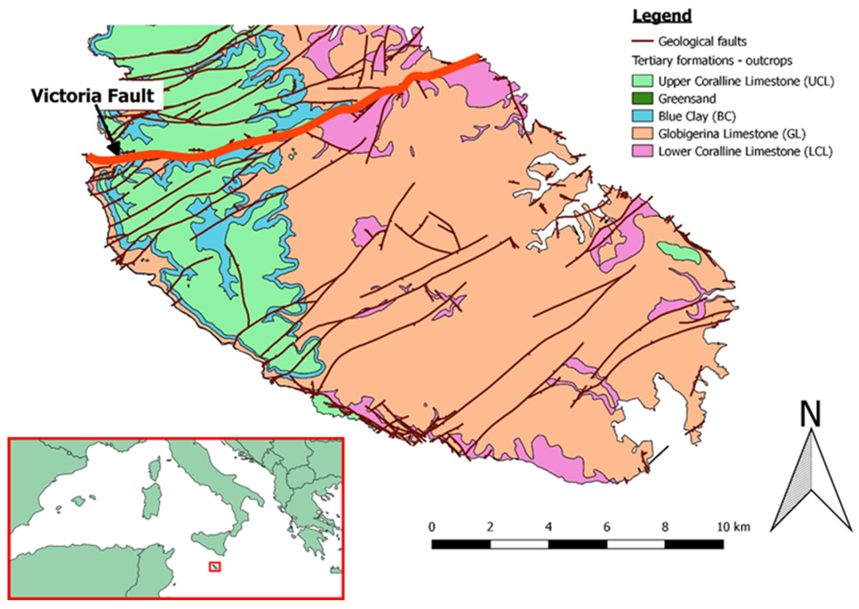
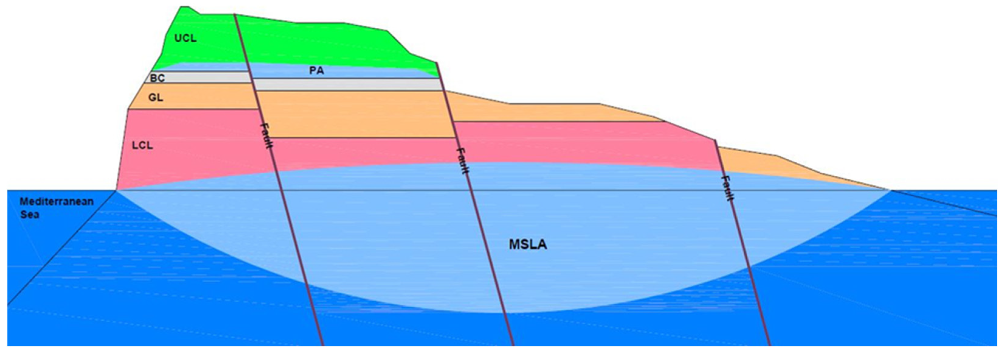
2.1. Study Area
- Plio-Quaternary; having little or no hydrogeological importance except possibly in alluvial valleys;
- Upper Coralline Limestone (UCL); characterised by fissured aquifers associated with a porous matrix. The UCL is a porous massive formation which outcrops over the western and northern zones of the Island and forms the highest parts of the topography. Well-developed karst phenomena can be found with dolines, sinkholes, weathered and corroded outcrops and fissures, dry valleys and dissolution figures;
- Greensand; a porous aquifer formation but of limited extent and usually very thin (less than 1 or 2 m);
- Blue Clay (BC); an aquitard formation sustaining an aquifer in the Greensand and UCL with possible vertical leakage enhanced by fissuration and faulting;
- Globigerina Limestone (GL); generally a massive and porous formation which is rather homogeneous all over the island;
- Lower Coralline Limestone (LCL); a fissured and fractured formation with a porous matrix. In the LCL, the main water body is in equilibrium with brackish and seawater. If compared to the GL formation, LCL is more fissured and entails higher heterogeneity due to a different deposition environment.
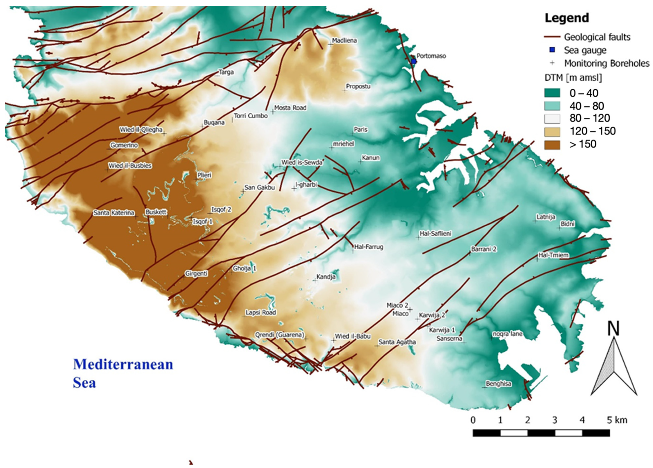
2.2. Monitoring System and Data Collection
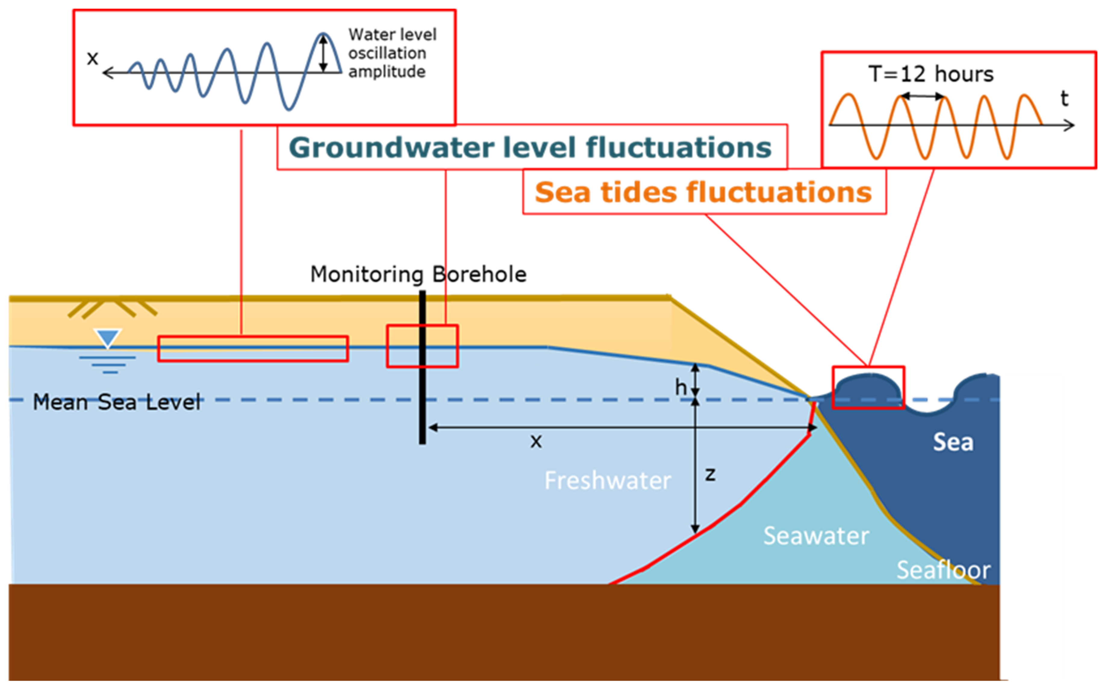
2.3. Tidal Attenuation
2.4. Geostatistical Analysis
3. Results
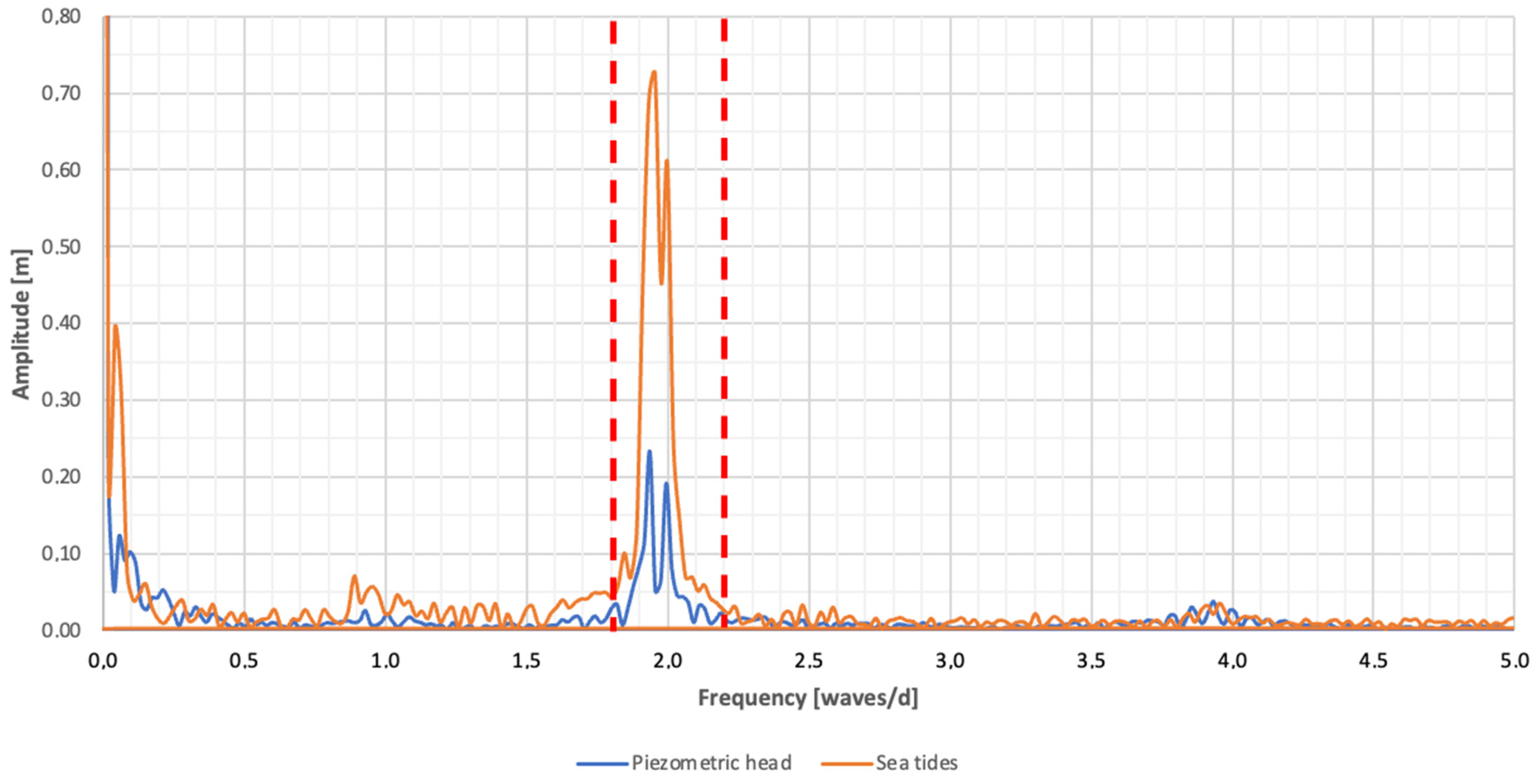
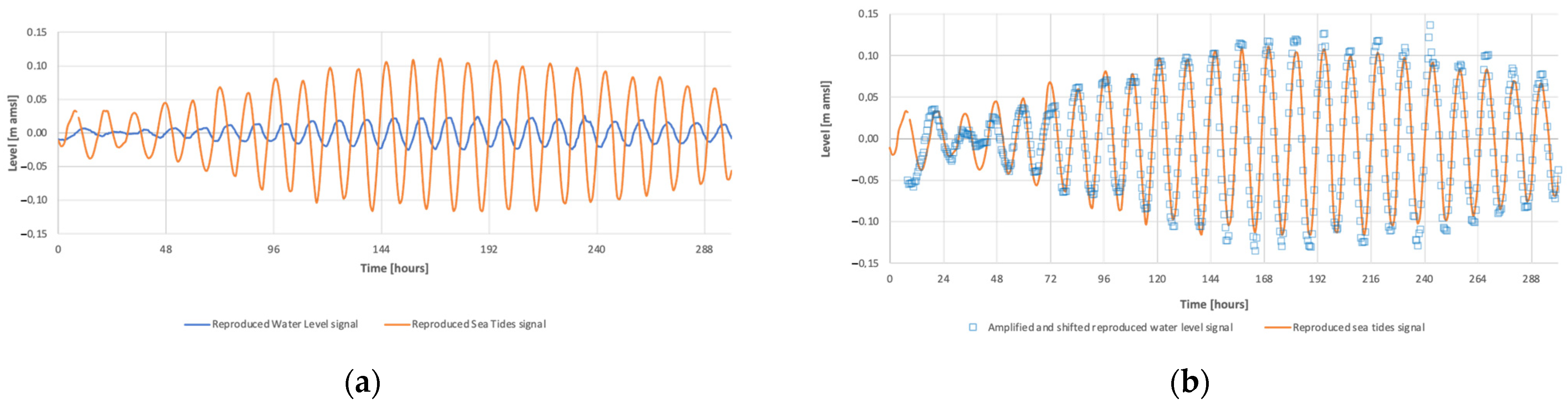
3.1. Tidal Analysis
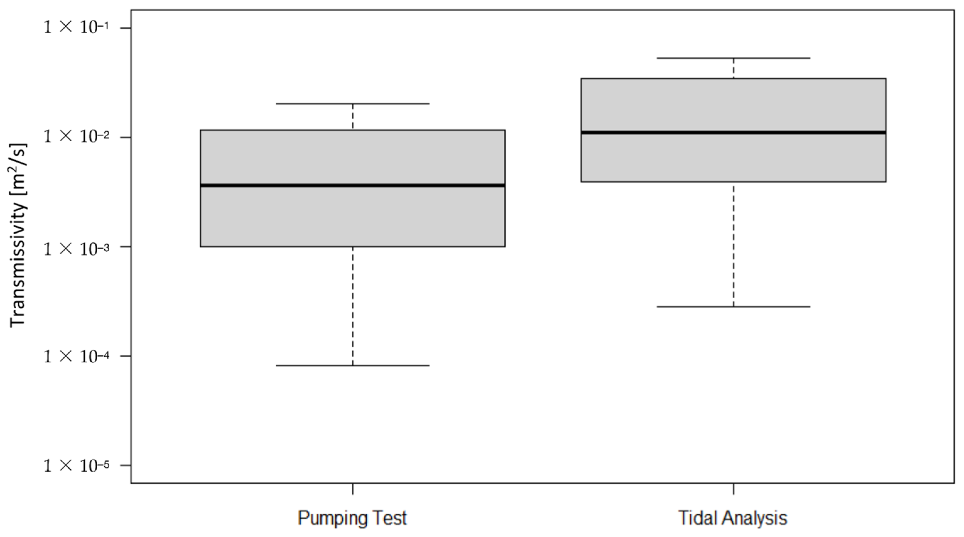
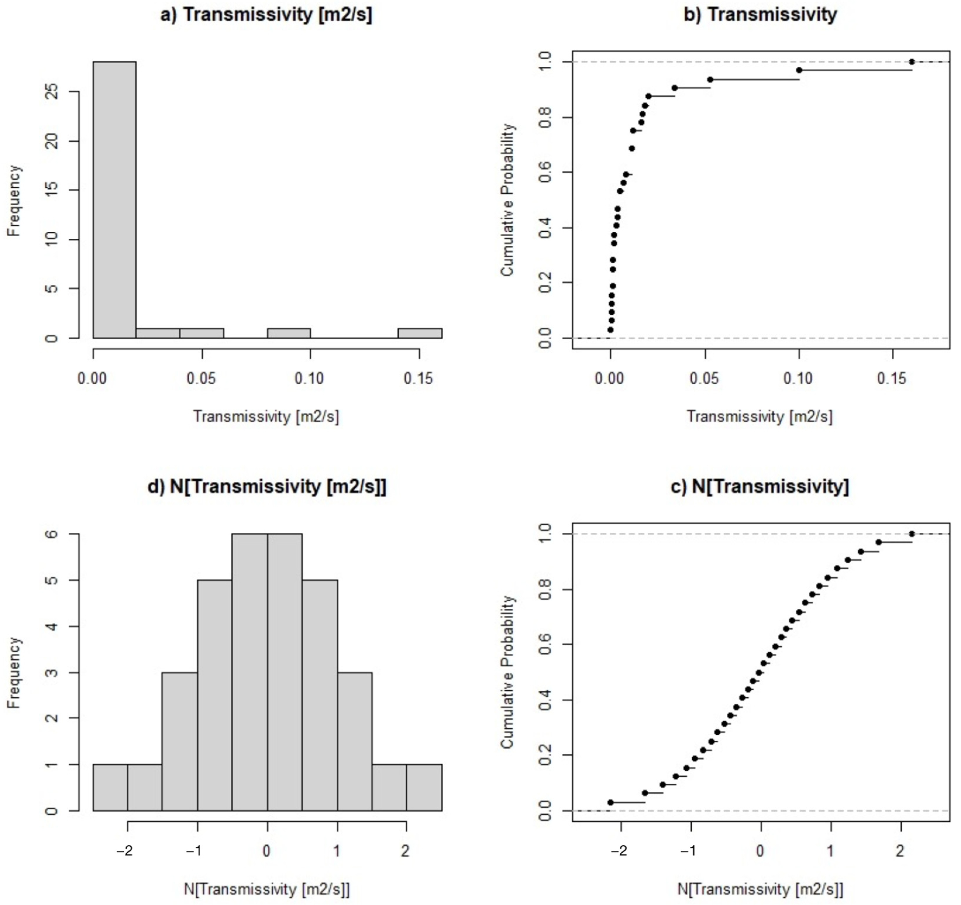
3.2. Geostatistical Analysis of Transmissivity
4. Discussion
5. Conclusions
Author Contributions
Funding
Data Availability Statement
Acknowledgments
Conflicts of Interest
References
- SEWCU (Sustainable Energy and Water Conservation Unit); ERA (Environmental and Resources Authority). The 2nd Water Catchment Management Plan for the Malta Water Catchment District 2015–2021; Government of Malta: Valletta, Malta, 2015; pp. 41–65, 107–124. [Google Scholar]
- Sapiano, M. Integrated Water Resources Management in the Maltese Islands. Acque Sotter. Ital. J. Groundw. 2020, 9. [Google Scholar] [CrossRef]
- Ortuño, F.; Molinero, J.; Custodio, E.; Juárez, I.; Garrido, T.; Fraile, J. Seawater intrusion barrier in the deltaic Llobregat aquifer (Barcelona, Spain): Performance and pilot phase results. In Proceedings of the SWIM21—21st Salt Water Intrusion Meeting, Barcelona, Spain, 21–26 June 2010; pp. 1–4. Available online: Swim-site.nl/pdf/swim21/pages_135_138.pdf (accessed on 15 November 2022).
- Javadi, A.A.; Hussain, M.S.; Abd-Elhamid, H.F.; Sherif, M.M. Numerical modelling and control of seawater intrusion in coastal aquifers. In Proceedings of the 18th International Conference on Soil Mechanics and Geotechnical Engineering, Paris, France, 6–9 September 2013; pp. 1–4. Available online: Cfms-sols.org/sites/default/files/Actes/739-742.pdf (accessed on 15 November 2022).
- Sinclair, K.M. ; National Centre for Groundwater Research and Training. Australian Groundwater Modelling Guidelines; Australian Government, National Water Commission: Turner, Australia, 2012; pp. 11–35. [Google Scholar]
- National Resource Management Ministerial Council; Environment Protection and Heritage Council; National Health and Medical Research Council. Australian Guidelines for Water Recycling, Managed Aquifer Recharge; National Water Quality Management Strategy Document No 24; Biotext: Canberra, Australia, 2009; pp. 33–52. ISBN 1921173475. [Google Scholar]
- BRGM. Study of the Fresh Water Resources of Malta; Services sol et sous-sol, Departement EAU: Paris, France, 1991; pp. 6, 74–77. [Google Scholar]
- Sánchez-Úbeda, J.P.; Calvache, M.L.; Duque, C.; López-Chicano, M. Estimation of hydraulic diffusivity using tidal-extracted oscillations from groundwater head affected by tide. In Proceedings of the 24th Salt Water Intrusion Meeting and the 4th Asia-Pacific Coastal Aquifer Management Meeting, Cairns, Australia, 4–8 July 2016; pp. 1–2. [Google Scholar]
- Rotzoll, K.; Gingerich, S.B.; Jenson, J.W.; El-Kadi, A. Estimating hydraulic properties from tidal attenuation in the Northern Guam Lens Aquifer, territory of Guam, USA. Appl. Hydrogeol. 2013, 21, 643–654. [Google Scholar] [CrossRef]
- Jacob, C.E. Flow of Groundwater. In Engineering Hydraulics; Rouse, H., Ed.; Wiley: Hoboken, NJ, USA, 1950; pp. 321–386. [Google Scholar]
- Ferris, J.G. Cyclic fluctuations of water level as a basis for determining aquifer transmissivity. Assoc. Int. Hydrol. Sci. 1951, 33, 148–155. [Google Scholar]
- Flinchem, E.P.; Jay, D.A. An introduction to Wavelet Transform Tidal Analysis Methods. Estuar. Coast. Shelf Sci. 2000, 51, 177–200. [Google Scholar] [CrossRef] [Green Version]
- Srzić, V.; Lovrinović, I.; Racetin, I.; Pletikosić, F. Hydrogeological Characterization of Coastal Aquifer on the Basis of Observed Sea Level and Groundwater Level Fluctuations: Neretva Valley Aquifer, Croatia. Water 2020, 12, 348. [Google Scholar] [CrossRef] [Green Version]
- Rahi, K.A. Estimating the Hydraulic Parameters of the Arbuckle-Simpson Aquifer by Analysis of Naturally-Induced Stresses. Ph.D. Thesis, Oklahoma State University, Stillwater, OK, USA, 2010. [Google Scholar]
- Ayers, J.F.; Clayshulte, R.N. A Preliminary Study of the Hydrogeology of Northern Guam; Technical Report No. 56; University of Guam, Water and Energy Research Institute of the Western Pacific: Mangilao, Guam, USA, 1984. [Google Scholar]
- Trefry, M.G.; Bekele, E. Structural characterization of an island aquifer via tidal methods. Water Resour. Res. 2004, 40, W01505. [Google Scholar] [CrossRef]
- Maréchal, J.C.; Hakoun, V.; Corbier, P. Role of Reef-Flat Plate on the Hydrogeology of an Atoll Island: Example of Rangiroa. Water 2022, 14, 2695. [Google Scholar] [CrossRef]
- Clark, W.E. Computing the barometric efficiency of a well. J. Hydraul. Div. 1967, 93, 93–98. [Google Scholar] [CrossRef]
- Turnadge, C.; Crosbie, R.S.; Barron, O.; Rau, G.C. Comparing Methods of Barometric Efficiency Characterization for Specific Storage Estimation. Groundwater 2019, 57, 844–859. [Google Scholar] [CrossRef]
- Rau, G.C.; Cuthbert, M.O.; Acworth, R.I.; Blum, P. Technical note: Disentangling the groundwater response to Earth and atmospheric tides to improve subsurface characterisation. Hydrol. Earth Syst. Sci. 2020, 24, 6033–6046. [Google Scholar] [CrossRef]
- McMillan, T.C.; Rau, G.C.; Timms, W.A.; Andersen, M.S. Utilizing the Impact of Earth and Atmospheric Tides on Groundwater Systems: A Review Reveals the Future Potential. Rev. Geophys. 2019, 57, 281–315. [Google Scholar] [CrossRef]
- Davis, D.R.; Rasmussen, T.C. A comparison of linear regression with Clark’s Method for estimating barometric efficiency of confined aquifers. Water Resour. Res. 1993, 29, 1849–1854. [Google Scholar] [CrossRef]
- Drogue, C. Coefficient D’infiltration ou Infiltration Efficace, sur les Roches Calcaires; Actes Colloque D’hydrologie en Pays Calcaire: Besançon, France, 1971; pp. 121–131. [Google Scholar]
- Mangin, A. Contribution à L’étude hydrodynamique des aquifères karstiques. Thèse Univ. Dijon. Ann. De Spéléologie 1975, 30, 21–124. [Google Scholar]
- Kiraly, L.; Müller, I. Hétérogénéité de la Perméabilité et de L’alimentation dans le Karst: Effet sur la Variation du Chimisme des Sources Karstiques [Heterogeneity of the Permeability and the Infiltration in the Karst: Effect on the Karstic Springs Water Chemistry Variations]; Bulletin du Centre d’Hydrogéologie: Neuchâtel, Switzerland, 1979; pp. 237–285. [Google Scholar]
- Williams, P.W. The role of the subcutaneous zone in karst hydrology. J. Hydrol. 1983, 61, 45–67. [Google Scholar] [CrossRef]
- Sauter, M. Quantification and Forecasting of Regional Groundwater Flow and Transport in a Karst Aquifer (Gallusquelle, SW Germany). Ph.D. Thesis, University of Tübingen, Tübingen, Germany, 1992. [Google Scholar]
- Klimchouk, A.B. ; The Formation of Epikarst and Its Role in Vadose Speleogenesis; National Speleological Society: Huntsville, AL, USA, 2000; pp. 91–99. [Google Scholar]
- Guo, H.; Jiao, J.J.; Li, H. Groundwater response to tidal fluctuation in a two-zone aquifer. J. Hydrol. 2010, 381, 364–371. [Google Scholar] [CrossRef]
- Rotzoll, K.; El-Kadi, A.I.; Gingerich, S.B. Estimating hydraulic properties of coastal aquifers using wave setup. J. Hydrol. 2008, 353, 201–221. [Google Scholar] [CrossRef]
- Magri, O. A geological and Geomorphological Review of the Maltese Islands with Special Reference to Coastal Zone; Territoris 4; Territoris Universitat de les Illes Belears: Palma, Spain, 2006. [Google Scholar]
- Herbert, P.T. The Geology of the Maltese Islands; Malta College of Arts, Science & Technology: Paola, Malta, 1955; pp. 22–33. [Google Scholar]
- Pedley, H.M. Syndepositional Tectonics Affecting Cenozoic and Mesozoic Deposition in the Malta and SE Sicily Areas (Central Mediterranean) and Their Bearing on Mesozoic Reservoir Development in the N Malta Offshore Region; Butterworth & Co, (Publishers) Ltd.: London, UK, 1989; pp. 171–178. [Google Scholar]
- Newbery, J. The Perched Water Table in the Upper Limestone Aquifer of Malta; Government of Malta: Valletta, Malta, 1968; pp. 551–570. [Google Scholar]
- OED (Oil Exploration Directorate, Office of the Prime Minister). Geological Map of the Maltese Islands: Sheet 1; Government of Malta: Valletta, Malta, 1993. [Google Scholar]
- Perrin, J. A Conceptual Model of Flow and Transport in a Karst Aquifer Based on Spatial and Temporal Variations of Natural tracers. Ph.D. Thesis, Centre of Hydrogeology, Universite de Neuchatel Faculte des Sciences Institute de Geologie, Neuchâtel, Switzerland, 2003; pp. 9–44. [Google Scholar]
- Real Time Stations @ Malta PORTOMASO. Available online: Ioi.research.um.edu.mt/capemalta/stations@malta/PORTOMASO/ (accessed on 19 November 2020).
- Backalowicz, M. Isotope Technology for Groundwater Development Hydrogeology of the Two Main Aquifers of Malta Island; Government of Malta: Valletta, Malta, 2001; Volume 3–6, pp. 13–14. [Google Scholar]
- ATIGA. Wastes Disposal and Water Supply Project, Malta; Interim Report on the Hydrology of Malta; ATIGA Consortium: Valletta, Malta, 1970. [Google Scholar]
- Morris, T. The Water Supply Resources of Malta; Government of Malta: Valletta, Malta, 1955; pp. 60–103. [Google Scholar]
- Tomasicchio, U. Manuale di Ingegneria Portuale e Costiera; Ulrico Hoepli Editore S.p.A.: Milan, Italy, 2015; pp. 76–82. [Google Scholar]
- Fidelibus, M.D.; Balacco, G.; Gioia, A.; Iacobellis, V.; Spilotro, G. Mass transport triggered by heavy rainfall: The role of endorheic basins and epikarst in a regional karst aquifer. Hydrol. Process. 2016, 31, 394–408. [Google Scholar] [CrossRef]
- Ghyben, B.W. Nota in Verband met de Voorgenomen Putboring Nabij Amsterdam. Tijdschr. Kon. Inst. Ing. 1888, 9, 8–22. [Google Scholar]
- Herzberg, A. Die Wasserversorgung einiger Nordseebäder. J. Gasbeleucht Wasserversorg 1901, 44, 815–819, 842–844. [Google Scholar]
- Guastaldi, E. Geostatistical Modeling of Uncertainty for the Risk Analysis of a Contaminated Site. J. Water Resour. Prot. 2011, 3, 563–583. [Google Scholar] [CrossRef] [Green Version]
- Gómez-Hernández, J.J.; Srivastava, R.M. One Step at a Time: The Origins of Sequential Simulation and Beyond. Math. Geosci. 2021, 53, 193–209. [Google Scholar] [CrossRef]
- Goovaerts, P. Geostatistics for Natural Resources Evaluation; Applied Geostatistics Series; Oxford University Press: Oxford, UK, 1997; Volume 14, p. 483. [Google Scholar]
- Barca, E.; Porcu, E.; Bruno, D.; Passarella, G. An automated decision support system for aided assessment of variogram models. Environ. Model. Softw. 2016, 87, 72–83. [Google Scholar] [CrossRef]
- Pebesma, E.; Graeler, B. Package ‘Gstat’. R News. 2021. Available online: Cran.r-project.org/web/packages/gstat/gstat.pdf (accessed on 15 November 2022).
- Isaaks, E.H.; Srivastava, R.M. An Introduction to Applied Geostatistics; Oxford University Press: Oxford, UK, 1989. [Google Scholar]
- El-Rawy, M.; De Smedt, F. Estimation and Mapping of the Transmissivity of the Nubian Sandstone Aquifer in the Kharga Oasis, Egypt. Water 2020, 12, 604. [Google Scholar] [CrossRef]


| Borehole Name | Locality | Distance to Sea [m] | Mean Hydraulic Head [m amsl] | Mean Depth to Water Level [m bGL] | Mean Amplitude [m] | Mean Period [hours] |
|---|---|---|---|---|---|---|
| Portomaso | Sea gauge | 0 | 0.042 | 0 | 0.069 | 12.43 |
| Noqra Lane | Birzebugga | 260 | 0.393 | 1.56 | 0.024 | 11.96 |
| Madliena | Gharghur | 1100 | 1.802 | 74.13 | 0.009 | 12.38 |
| Hal-Tmiem | Zejtun | 1680 | 2.498 | 46.12 | 0.014 | 12.34 |
| Karwija | Safi | 2600 | 1.553 | 76.68 | 0.016 | 12.37 |
| Wied Busbies | Rabat | 2675 | 2.115 | 158.93 | 0.010 | 12.27 |
| Barrani | Ghaxaq | 4500 | 1.953 | 38.79 | 0.012 | 12.10 |
| Wied Sewda | Attard | 4600 | 2.107 | 55.29 | 0.013 | 12.30 |
| Mosta Road | Mosta | 5150 | 1.955 | 68.54 | 0.032 | 12.39 |
| Buqana | Mosta | 7750 | 2.347 | 87.83 | 0.010 | 12.15 |
| Borehole Name | Locality | Distance to Sea [m] | D [m2/s] | T [m2/s] | b [m] | K [m/s] |
|---|---|---|---|---|---|---|
| Noqra Lane | Birzebugga | 260 | 7 | 2.8 × 10⁻⁴ | 14 | 2.1 × 10⁻⁵ |
| Madliena | Gharghur | 1100 | 29 | 1.5 × 10⁻³ | 61 | 2.4 × 10⁻⁵ |
| Hal-Tmiem | Zejtun | 1680 | 78 | 3.9 × 10⁻³ | 92 | 4.3 × 10⁻⁵ |
| Karwija | Safi | 2600 | 221 | 1.1 × 10⁻² | 57 | 1.9 × 10⁻⁴ |
| Wied Busbies | Rabat | 2675 | 139 | 6.9 × 10⁻³ | 78 | 8.9 × 10⁻⁵ |
| Barrani | Ghaxaq | 4500 | 323 | 1.6 × 10⁻² | 72 | 2.3 × 10⁻⁴ |
| Wied Sewda | Attard | 4600 | 685 | 3.4 × 10⁻² | 77 | 4.4 × 10⁻⁴ |
| Mosta Road | Mosta | 5150 | 4431 | 1.6 × 10⁻¹ | 72 | 2.2 × 10⁻³ |
| Buqana | Mosta | 7750 | 1069 | 5.3 × 10⁻² | 86 | 6.2 × 10⁻⁴ |
| Parameter | Symbol | Units | Value |
|---|---|---|---|
| Mean | m2/s | 0.016 | |
| Variance | - | 0.001 | |
| Nugget | - | 0.480 | |
| Sill | - | 0.600 | |
| Range | m | 4005 |
Disclaimer/Publisher’s Note: The statements, opinions and data contained in all publications are solely those of the individual author(s) and contributor(s) and not of MDPI and/or the editor(s). MDPI and/or the editor(s) disclaim responsibility for any injury to people or property resulting from any ideas, methods, instructions or products referred to in the content. |
© 2023 by the authors. Licensee MDPI, Basel, Switzerland. This article is an open access article distributed under the terms and conditions of the Creative Commons Attribution (CC BY) license (https://creativecommons.org/licenses/by/4.0/).
Share and Cite
Demichele, F.; Micallef, F.; Portoghese, I.; Mamo, J.A.; Sapiano, M.; Schembri, M.; Schüth, C. Determining Aquifer Hydrogeological Parameters in Coastal Aquifers from Tidal Attenuation Analysis, Case Study: The Malta Mean Sea Level Aquifer System. Water 2023, 15, 177. https://doi.org/10.3390/w15010177
Demichele F, Micallef F, Portoghese I, Mamo JA, Sapiano M, Schembri M, Schüth C. Determining Aquifer Hydrogeological Parameters in Coastal Aquifers from Tidal Attenuation Analysis, Case Study: The Malta Mean Sea Level Aquifer System. Water. 2023; 15(1):177. https://doi.org/10.3390/w15010177
Chicago/Turabian StyleDemichele, Francesco, Fabian Micallef, Ivan Portoghese, Julian Alexander Mamo, Manuel Sapiano, Michael Schembri, and Christoph Schüth. 2023. "Determining Aquifer Hydrogeological Parameters in Coastal Aquifers from Tidal Attenuation Analysis, Case Study: The Malta Mean Sea Level Aquifer System" Water 15, no. 1: 177. https://doi.org/10.3390/w15010177