Chemodynamics of Mercury (Hg) in a Southern Reservoir Lake (Cane Creek Lake, Cookeville, TN, USA): I—Estimation of the Kinetics of Photochemical Reduction of Aquatic Hg(II) Using Field-Measured Data of Hg Water/Air Exchange and Dissolved Gaseous Hg

Abstract

An alternative, independent estimation of the kinetics of aquatic Hg(II) photochemical reduction featuring dissolved gaseous mercury (DGM) emission from water in consideration was obtained by using a mass balance box model. An interactive Excel spreadsheet was constructed to implement the model equations to yield the rate constants and the rates of the Hg(II) photoreduction. The model calculations used field-measured data of DGM paired with its emission flux coupled with the corresponding field sampling times. This data set came from a previous, separate, year-long field study conducted at a southern reservoir lake (Cane Creek Lake, Cookeville, Putnam County, TN). The mean value of the model-calculated rate constants (k_DGM) of the Hg(II) photoreduction for the warm season (June–August) (4.5 fM h⁻¹/pg L⁻¹) is higher than that for the cold season (October–January) (2.2 fM h⁻¹/pg L⁻¹). The rate constants were found to be the highest (22.5 fM h⁻¹/pg L⁻¹) in August whereas the lowest (0.03 fM h⁻¹/pg L⁻¹) in January. The model-calculated rate constants are clearly higher in value than but comparable in order of magnitude to the published kinetic data. The model-calculated rates (r_DGM) of the Hg(II) photoreduction are significantly higher, by one order of magnitude (10² vs. 10¹) than the apparent rates calculated using the same field DGM data without consideration of the Hg emission from the water. A sensitivity analysis of the model parameters points to a high sensitivity of Hg emission flux to the rate constant under modeled realistic environmental conditions. The initial Hg(II) concentration is also a sensitive model parameter under certain conditions. The results of our model study support the conclusion that DGM emission from water has a strong impact on the kinetics of aquatic Hg(II) photoreduction and the model calculation can provide an independent, valuable approach for estimating the kinetics of aquatic Hg(II) photoreduction.

1. Introduction

The global, persistent, toxic, and bioaccumulative nature of mercury (Hg) necessitates a better and deeper understanding of its transformation and transport so as to unveil its fate in the environment [1] The three major forms of aquatic mercury are elemental Hg (Hg(0)), inorganic divalent Hg (Hg(II)), and methylated Hg (CH₃Hg⁺, (CH₃)₂Hg). Hg(II), bonded to various organic and inorganic ligands, is the dominant form of aquatic Hg [2]. The production of aqueous Hg(0)_g, operationally defined as dissolved gaseous mercury (DGM), has been linked to the reduction of Hg(II) (Hg(II) + 2e⁻ ⇔ Hg(0)) (e.g., [3]). DGM is the main source of Hg evasion (emission) at the air/water interface and thus linked to the global cycle of Hg [4]. Hg(II) species that are not reduced to Hg(0) can undergo methylation to become methylated Hg such as CH₃Hg⁺, a known neuro-toxin. DGM is therefore a highly important intersectional component in the aquatic biogeochemical cycle of Hg as it may lessen the amount of Hg(II) available for methylation and ultimately bioaccumulation up the food chain [5].

There have been a growing number of studies on the reduction of Hg(II) in aquatic systems (e.g., [2,3,6,7,8,9,10,11]). It has been established that sunlight can strongly mediate and enhance the reduction and control aquatic Hg redox cycle between Hg(II) and Hg(0) (e.g., [2,3,7,8]). Solar radiation has also been pinpointed to be a major driving force in controlling and enhancing Hg evasion from waters (e.g., [12,13,14]). While the number of studies on aquatic photochemokinetics of Hg has been rapidly rising (e.g., [2,8,15,16]), detailed, well-understood mechanisms of the aquatic Hg photoredox cycle still remain a gap to be filled [9], although progresses have been made along this line [10,11].

A sound mechanistic understanding of aquatic Hg photoredox requires a good knowledge of the kinetics of the Hg photoredox. The data of rates and rate constants of aquatic Hg photoreduction have been steadily growing (e.g., [9,11]). The published data were obtained from field studies or lab simulation experiments. These either could under-estimate the real kinetics as a result of use of closed experimental systems excluding the Hg emission from waters (e.g., [3,7]), or could lead to over-estimates stemming from enhanced purging of DGM (e.g., [2,8]) in simulation experiments. Some kinetic data were obtained by tracking the temporal change of DGM concentrations [16]. This approach, however, may also underestimate the real kinetics for the same reason of absence of consideration of aquatic Hg emission.

Yet, it is actually very difficult and challenging to obtain real kinetics of aquatic Hg photoreduction in situ or in the laboratory under authentic field conditions with aquatic Hg emission in play. In this paper, we report an effort to explore using modeling as an alternative approach to estimating the kinetic rate constants and rates of aquatic Hg(II) photoreduction. Moreover, this model considers the Hg emission by using authentic DGM and Hg emission flux data obtained in situ concurrently. In particular, we used a mass balance box model to calculate and estimate the aquatic Hg(II) photoreduction kinetics. Previously a year-long field study was carried out to concurrently obtain DGM and Hg emission flux data [13,14] in a southern lake (Cane Creek Lake, Cookeville, TN, USA). To our best knowledge, this appears to be the single existing data set with paired data of concurrent DGM and Hg emission flux available over a year-long period of time covering various seasons. This then allowed us to be able to carry out our model study of such a kind and to examine the seasonal trends of the Hg(II) photoreduction kinetics in the lake.

The major objectives of this model study were (1) to construct a useful model that can be employed to calculate aquatic Hg photoreduction rate constants and rates with Hg air/water exchange considered, (2) to provide an alternative, independent estimation of aquatic Hg photoreduction kinetics to compare with the published kinetic data, and (3) to investigate the role of Hg emission in aquatic Hg photoreduction. Ultimately, this endeavor was aimed at answering the question concerning whether Hg emission affects aquatic Hg photoreduction or not and the potential err and its degree in estimation of aquatic Hg photoreduction kinetics.

2. Model Construction and Description

The current models of aquatic Hg chemodynamics consider either Hg transport or transformation, usually with the two treated separately (e.g., [2,8,13,14]). There is a lack of cooperation of both Hg air/water exchange and photoredox transformation in one single model to treat aquatic Hg photochemodynamics comprehensively. One attempt to fill the gap was the use of a mass balance box model with both the transformation and the transport built in [17]. In the present study, our model was then adapted from this model of Zhang and Lindberg [17] and built to provide an interactive spreadsheet that computes the rate constants and the rates of aquatic Hg photo-reduction at given time periods. This approach addresses some concerns regarding the investigation into aquatic Hg chemodynamics.

One concern involves the application of simple regular empirical kinetic laws or kinetic models (e.g., first-order or second-order kinetics) to aquatic systems for Hg redox cycle. The use of these regular kinetic models prescribes the requirement of a closed system for a particular Hg species. Hence, caution needs to be exercised upon a use of these kinetic models and the subsequent interpretation of the results when a real open aquatic system in the field is dealt with. The best, rigorous approach is an adoption of a mass balance for Hg with both transformation and transport considered.

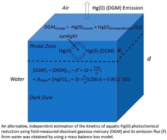
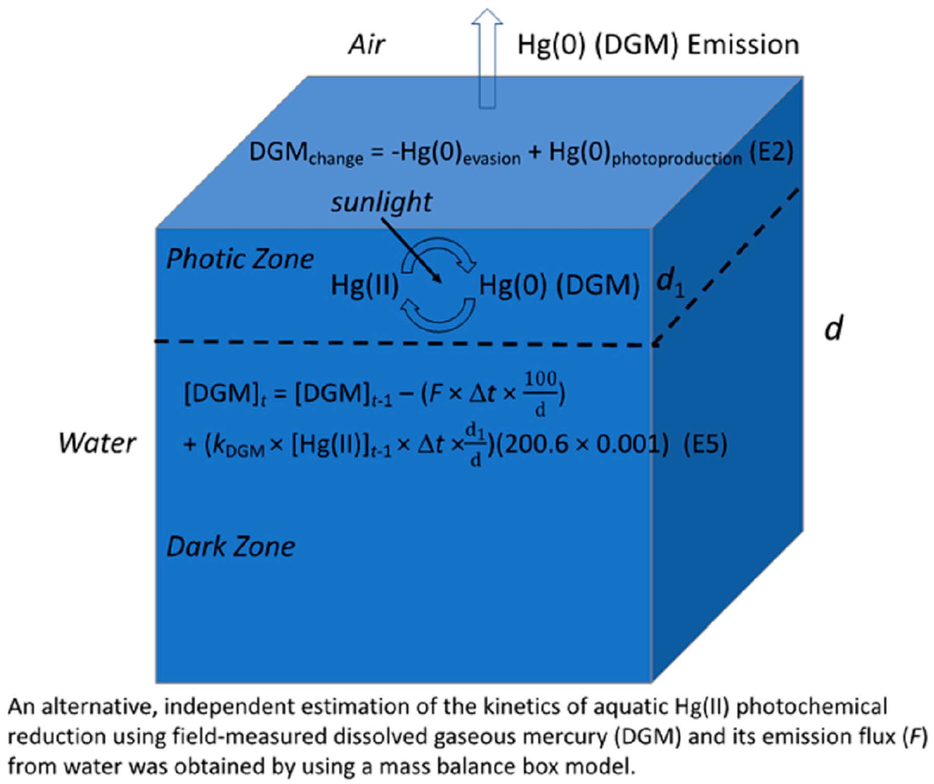
The model adaptation is described as follows (for more details, see [18]). Our model used the same DGM budget (see (1)) based on a Hg mass balance in a box representing a water column [17]. The box (total depth d), as assumed, has two sub-compartments: a surface photic zone (depth d₁), in which sunlight is readily available and photoreduction proceeds actively, and a dark zone below, in which sunlight is scarce (Figure 1). The general mass balance equation for Hg in Equation (1) is given below [17]:

$${\mathrm{DGM}}_t{=\mathrm{DGM}}_{t-1} - \mathrm{Evasion}+\mathrm{DGM} \mathrm{production} -{ \mathrm{Hg}}^0 \mathrm{oxidation}$$

(1)

Our model also adopted two major assumptions: (1) absence of new Hg inputs into the box (e.g., atmospheric deposition, exchange at water/sediment interface, water flow and runoff, since compared to the Hg(II) photoreduction, these inputs are significantly slower or ignorable) and (2) an overall apparent first-order kinetics of Hg(II) photoreduction [17]. Incidentally, the mixing in the box was assumed to be immediate, instant, and complete. The DGM produced in the photic zone thus can be well mixed in the entire box immediately, instantly, and completely. For simplicity, aquatic Hg (photo)oxidation was excluded in the model, which is probably reasonable for sunny daytime in various cases when Hg photoreduction generally predominates [17]. Under these assumptions, the final model equations to compute the rate constants and the rates of aquatic Hg(II) photo-reduction (i.e., Hg(0) photo-generation or photo-production) at given time periods can be derived from the general Hg balance Equation (1) as shown below in details.

First of all, a rigorous mass balance model for DGM in the box is given as:

DGM_change = −Hg(0)_evasion + Hg(0)_{photoproduction}

(2)

$$\mathrm{d}[\mathrm{DGM}](t)=-F(t)(\mathrm{d}t)(\frac{100}{d})+k_{\mathrm{DGM}}(t)[\mathrm{Hg}(\mathrm{II})](t)(\mathrm{d}t)(\frac{d_1}{d})(200.6 \times 0.001)$$

(3)

Since F(t), k_DGM(t), and [Hg(II)](t) are changing with time and these complicated functions are thus unavailable, a certain approximation thus can lead to:

$$\mathsf{\Delta }[\mathrm{DGM}](t)=F(t)(\mathsf{\Delta }t)(\frac{100}{d})+k_{\mathrm{DGM}}(t)[\mathrm{Hg}(\mathrm{II})](t)(\mathsf{\Delta }t)(\frac{d_1}{d})(200.6 \times 0.001)$$

(4)

Considering Δ[DGM](t) = [DGM]_t − [DGM]_t−1, we have:

$${[\mathrm{DGM}]}_t={[\mathrm{DGM}]}_{t-1}-(F \times \mathsf{\Delta }t \times \frac{100}{d})+(k_{\mathrm{DGM}} \times {[\mathrm{Hg}(\mathrm{II})]}_{t-1} \times \mathsf{\Delta }t \times (\frac{d_1}{d})(200.6 \times 0.001)$$

(5)

The above Equation (5) is then the one ready to be rearranged to yield the equations to compute the rate constants and the rates of aquatic Hg photo-reduction at given time periods.

The terms in (5) are defined and discussed as follows. [${\mathrm{DGM}}_{\mathrm{t}}$](pg L⁻¹) is the DGM concentration at the current period Δt and [${\mathrm{DGM}}_{\mathrm{t}-1}$] (pg L⁻¹) is the one at the immediate previous period. Initially, [DGM]₀ = [DGM]_{0, t0}, which is the initial DGM concentration at t = 0. F (ng m⁻² h⁻¹) is the mean evasion (emission) flux at the current period. Δt (h) is the time interval for each period in which DGM and flux data were collected concurrently. All the data of the DGM ([DGM]), Hg emission flux (F), and corresponding time period for the DGM and F (at Δt) used in the model calculations are authentic field data provided by a previous field study as mentioned before [13,14].

In addition to the real field data, several (adjustable) model parameters were also enlisted. d (cm) is the total depth of the box for the modeled water column. The value of 100 is a conversion factor for use of cm as the unit for d. k_DGM (fM h⁻¹/pg L⁻¹), to be calculated, is the pseudo first-order rate constant for DGM production at the current period. ${[\mathrm{Hg}(\mathrm{II})]}_{\mathrm{t}-1}{(\mathrm{pg} \mathrm{L}}^{-1})$ is the dissolved reactive mercury (DRM) concentration at the previous period. $\frac{d_1}{d}$ is the ratio of the depth of the surface photic zone (d₁) to the total depth of the box (water column, d). The constant 200.6 (g mol⁻¹) is the atomic mass of elemental Hg. The value of 0.001 is the factor for conversion from femtograms (10⁻¹⁵ g) to picograms (10⁻¹² g). The terms of DGM production (generation) and Hg(II) photoreduction (photochemical reduction) are used interchangeably.

Now, the above model Equation (5) can be readily rearranged to solve for k_DGM to yield the DGM production rate constant (${\mathrm{k}}_{\mathrm{DGM}}$ in [(fM h⁻¹)/(pg L⁻¹)]) using the Equation (6) below:

$$k_{\mathrm{DGM}} [(\mathrm{fM} {\mathrm{h}}^{-1})/(\mathrm{pg} {\mathrm{L}}^{-1})]=\frac{{\mathrm{DGM}}_{t }-{ \mathrm{DGM}}_{t-1}+(F \times \mathsf{\Delta }t \times \frac{100}{d})}{{[\mathrm{Hg}(\mathrm{II})] }_{t-1} \times \mathsf{\Delta }t \times \frac{d_1}{d} \times 0.2006}$$

(6)

The [Hg(II)] at the current period ([Hg(II)]_t) can be calculated using the following equation:

$${[\mathrm{Hg}(\mathrm{II})]}_t={[\mathrm{Hg}(\mathrm{II})]}_{t-1} - k_{\mathrm{DGM}} \times {[\mathrm{Hg}(\mathrm{II})]}_{t-1} \times (\mathsf{\Delta }t) \times (\frac{d_1}{d}) \times (0.2006)$$

(7)

where [Hg(II)]_t−1 = [Hg(II)]₀, initial Hg(II) concentration, at t = 0.

Next, the model-calculated aquatic Hg(II) photoreduction rate (r_t in fM h⁻¹) can be obtained by Equation (8) given below (assuming pseudo first-order kinetics for the Hg(II) reduction):

r_t (fM h⁻¹) = k_DGM[Hg(II)]_t−1

(8)

where fM h⁻¹ is the unit used for our model study.

This unit can be converted to the unit commonly used (i.e., pg L⁻¹ h⁻¹) to compare with other published rates (fM h⁻¹ × 0.2006 = pg L⁻¹ h⁻¹).

Last, in addition, the apparent rate (apparent r_t in pg L⁻¹ h⁻¹) of the Hg(II) photoreduction or DGM generation can be calculated by Equation (9) below adopted from Zhang and Dill [16] using the same field DGM data set (from the same field study described previously):

$$\mathit{apparent} {r_t}_{ }(\mathrm{pg} {\mathrm{L}}^{-1} {\mathrm{h}}^{-1})=\frac{\Delta [\mathrm{DGM}]}{\Delta t}=\frac{{([\mathrm{DGM}]}_t{ -[\mathrm{DGM}]}_{t-1})}{\Delta t}$$

(9)

At this point, certain elaborations need to be made as follows:

Frist of all, the k_DGM (fM h⁻¹/pg L⁻¹) in the model should be viewed as an overall rate constant (k_DGM = Σk_DGMi). This may be seen in two perspectives. Firstly, this rate constant may be interpreted as the one for Hg(II) reduction only under the assumption of an absence of Hg(0) oxidation (oxidation ignored or at minimum). Secondly, it may be interpreted as a net overall rate constant that includes both the reduction and oxidation. Both interpretations can be plausible. The first may be more appropriate in the morning when Hg(0) production is predominant while the oxidation is minimum or slow. The second may be more relevant near noon time and in the afternoon when Hg(0) has built up and thus its oxidation becomes faster.

Incidentally, there could be a number of reactions that are responsible for the observed overall Hg redox transformation. However, the model would become much complicated if each individual reaction is considered. Hence, this model treats all the participating reactions combined together as if in one single apparent overall reaction. Furthermore, k_DGM is actually changing with time, because it contains a component associated with sunlight (i.e., k_DGM = f(sunlight intensity)) as a result of the photochemical nature of the aquatic Hg redox. Thus, all things considered, the model-calculated rate constant actually represents an overall rate constant that incorporates all the contributions (controlling factors) to the Hg transformation under field conditions (Hg redox, sunlight, Hg emission, etc.).

The parameter of k_DGM (fM h⁻¹/pg L⁻¹) in the model originates from a model assumption that the aquatic Hg(II) reduction to generate DGM can be treated kinetically as an apparent first-order reaction overall. This plausible assumption is based on the notion that the level of the aquatic reductants for Hg(II) is significantly higher than that of aquatic reducible Hg(II). This notion has been observed in various studies on aquatic Hg(II) reduction (e.g., [2,3,9]). This assumption leads to r_t = k[Hg(II)][reductants] = k_DGM[Hg(II)] (8), where k_DGM = k[reductants] since [reductants] can be approximately treated as a constant following the notion mentioned above.

Second, although an assumption was adopted of no Hg inputs into the box (e.g., from deposition, sediments, lake turnover, water flow, runoff, etc.), the model parameter [Hg(II)]₀ may be linked to, and thus reflect, these Hg inputs. This is because presumably an occurrence of any of these input events would lead to a change of the initial Hg(II) concentration ([Hg(II)]₀) for the model calculation. Hence, [Hg(II)]₀ actually embeds these inputs in this model parameter.

Third, it is known that the boundary between the surface photic zone and the bottom dark zone is actually not distinct but rather involves a continuous gradual transition. A distinct boundary was still assumed, however, for simplicity, which thus leads to a clear distinct depth (d₁) of the photic zone in the model.

Last, the k_DGM calculated using the model retains a unit of (fM h⁻¹)/(pg L⁻¹) for convenience of the present model study. However, the k_DGM values in this model unit were also converted (by timing a factor of 0.2006) to the values in the common unit for first-order kinetics (i.e., h⁻¹) for appropriate comparison with the published values from various other studies.

An Excel spreadsheet was readily set up to carry out the model calculations given the model parameters as selected. For most of the model calculations, the values of the model parameters used were 2 m (200 cm) for d (the depth for Cane Creek Lake [19]) and 0.01 m (10 cm) for d₁ [17]. The value of [Hg(II)]₀ selected was 150 pg L⁻¹, which is a reasonable assumption for a common unpolluted system such as Cane Creek Lake [19]. Other values of d, d₁, and [Hg(II)]₀ were also used in the model sensitivity study as appropriate.

It needs to be pointed out that as a distinct feature of this model study, concurrent DGM concentration and Hg emission flux data together with the corresponding Δt data used for the model calculations are all real field data obtained from a previous field study [13,14]. This provides the sole data set available and thus is not only highly valuable but also required for the model study of such a kind. The field data of DGM, flux, and Δt used are (must be) all coupled with both DGM and flux obtained in the same period of Δt. Consequently, the data of paired DGM and flux available and qualified for the model calculations were not as ample as expected. There were some negative rate constants as a result of fluctuation of the field data and so these were thus excluded from the model study [18].

The model-calculations depend on the DGM concentrations and Hg(0) emission fluxes with respect to the accuracy and uncertainty. In this study, the calculated rate constants and rates are reported either in one decimal digit (e.g., x.x, xx.x, etc.) or in two significant figures (e.g., 0.xx, 0.0xx, etc.), whichever is more applicable. This treatment stems from a conservative assessment of the overall accuracy and uncertainty of the field-obtained DGM concentrations and Hg(0) emission fluxes [13,14,18].

3. Results and Discussion

In this study, the rate constants (k_DGM), [Hg(II)], and rates (r_t) of the Hg(II) photoreduction were calculated using an interactive Excel spreadsheet composed of the model Equations (6)–(8) together with the coupled DGM and flux data obtained from a separate field study [13,14] (

Table 1. Rate constants and rates of aquatic DGM photoproduction calculated by a simple mass balance box model and apparent rates of the DGM production calculated from DGM concentrations from field measurements.

Date	Time (EST)	[Hg(II)]	kDGM	kDGM	Model rDGM	Apparent rDGM	Twater	Rg	UVA
	(h)	(pg L−1)	(fM h−1/pg L−1)	(h−1)	(pg L−1 h−1)	(pg L−1 h−1)	(°C)	(W m−2)	(μW cm−2)
8 June 2004	13.83	137.1	6.5	1.3	194.4	7.8	28	746.4	605
	15.17	119.3	9.7	1.9	265.5	11.8	30	632.5	1680
	17.83	117.5	6.7	1.3	172.8	7.6	29	567.6	688
	20.50	118.3	0.27	0.055	6.5	−0.08	26	84.2	88
22 June	17.42	157.9	5.6	1.1	191.2	9.0	30	604.9	1210
9 July	18.50	192.6	6.4	1.3	269.5	13.0	32	416.2	520
15 July	12.50	146.3	1.8	0.37	55.2	1.7	30	826.1	1740
	13.83	145.9	0.21	0.043	6.3	−0.56	31	783.9	660
	15.17	143.1	1.4	0.28	41.2	1.1	32	771.6	2210
	18.50	164.1	1.8	0.37	61.7	2.3	31	431.9	390
3 August	15.33	142.9	3.5	0.71	106.2	4.3	31	860.5	1700
	16.00	121.3	22.5	4.5	646.0	31.2	31	768.5	1130
4 August	12.92	150.4	1.1	0.21	32.6	0.82	30	850.2	1500
	16.25	149.3	0.74	0.15	22.4	0.35	31	732.4	960
	17.58	132.3	8.6	1.7	256.4	12.1	31	512.7	470
5 August	17.42	155.7	0.077	0.015	2.4	−0.18	29	174.6	160
	19.42	155.0	0.23	0.045	7.1	0.070	28	185.6	80
29 October	13.58	148.4	0.80	0.16	24.2	0.49	22	627.8	370
	16.25	148.9	1.8	0.35	53.8	2.2	22	324.8	330
	17.58	139.4	4.8	0.96	143.2	6.8	21	187.7	170
	18.25	138.7	0.69	0.14	19.2	0.78	21	120.5	20
5 November	13.83	155.4	1.6	0.33	51.7	2.4	18	554.4	380
3 December	13.67	155.5	5.9	1.2	191.3	9.2	10	516.41	0.24
21 January 2005	12.67	144.2	1.9	0.38	57.7	2.8	7	479.7	0.14
	14.00	144.2	0.030	0.0060	0.87	−0.24	7	507.5	0.15

[Hg(II)]t = Hg(II) concentration at time period t calculated using model Equation (7); kDGM = model—calculated rate constant of DGM photoproduction using model Equation (6); model r_t: rate of Hg(II) photoreduction calculated using model Equation (8); apparent rDGM = apparent rate of DGM photoreduction calculated using Equation (9); Rg = solar radiation; UVA = UVA radiation. model parameters in the model Equation (6) used for calculations: F and DGM = real field data, [Hg(II)]0 = 150 pg L⁻¹, d = 200 cm, d₁ = 10 cm.

). The effects of environmental factors such as water temperature and solar radiation on the Hg(II) photoreduction kinetics were then investigated to examine the nature and driving force of the Hg(II) photoreduction. We also calculated the apparent rates of real DGM production to compare these with the model-calculated rates to look into the role of Hg emission on the Hg(II) photoreduction. A model sensitivity study was conducted to inspect the sensitivity of major model parameters. A detailed documentation of this model study is available elsewhere [18].

3.1. Model Calculation of the Rate Constants of the Hg(II) Photoreduction

Using the coupled field data of DGM and Hg emission flux, we obtained model-calculated kinetic rate constants of the Hg(II) photoreduction for the period from summer to winter (June–January), covering a wide seasonal span including warm and cold seasons (Table 1 and

Table 2. Summary of the daily DGM production rate constant values (kDGM) calculated using the simple mass balance box model.

Date	Time Span	Daily Mean kDGM	Daily Max. kDGM	Daily Min. kDGM	Number of Daily kDGM
	(EST)	[(fM h−1)/(pg L−1)]	[(fM h−1)/(pg L−1)]	[(fM h−1)/(pg L−1)]
8 June 2004	12.50–20.50	5.8	9.7	0.27	4
22 June	12.08–18.75	5.6	-	-	1
9 July	13.17–18.50	6.4	-	-	1
15 July	11.17–18.50	1.3	1.8	0.21	4
3 August	14.00–0.67	13.0	22.5	3.5	2
4 August	8.25–20.92	3.5	8.6	0.74	3
5 August	11.42–19.42	0.15	0.23	0.077	2
29 October	12.25–18.25	2.01	4.8	0.69	4
5 November	11.83–17.17	1.6	-	-	1
3 December	12.33–15.67	5.9	-	-	1
21 January 2005	10.67–16.67	0.97	1.9	0.03	2

). The rate constants (k_DGM) are presented in both the unit of (fM h⁻¹)/(pg L⁻¹) for convenient model study and the unit of h⁻¹ for direct comparison with published data (Table 3). The magnitude of the Hg(II) reduction rate constants was found for each of the sampling days, and a summary of the daily results is provided in Table 2.

The rate constants for the first half of the sampling period (June–August) are significantly higher than for the second half (October–January). The months of June through August see an average rate constant (k_DGM) range of 1.3–13.0 [(fM h⁻¹)/(pg L⁻¹)], a minimum daily range of 0.21–3.5 [(fM h⁻¹)/(pg L⁻¹)], and a maximum daily range of 1.8–22.5 [(fM h⁻¹)/(pg L⁻¹)]. An exception is August 5, which has a daily average of 0.15, a min. of 0.077, and a max. of 0.23 [(fM h⁻¹)/(pg L⁻¹)]. During the cold weather months (October–January), the rate constants are considerably lower. During this time period, the average daily rate constant values range from 0.97 to 5.9 [(fM h⁻¹)/(pg L⁻¹)], with the minimum daily values of 0.03–0.69 and the maximum of 1.9–4.8 [(fM h⁻¹)/(pg L⁻¹)].

Some of the rate constant data are presented in Figure 2a for the warm season and Figure 2b for the cold season to show the general magnitude of the kinetics and a handy comparison of the kinetics between the warm and cold seasons. The model-calculated Hg(II) reduction rate constants vary mildly from day to day, as naturally did the solar and UVA radiation whereas the water temperature remained nearly unchanged.

The calculated rate constants clearly show a seasonal variation, with the values of the warm season (June–August) (Mean: 4.5 fM h⁻¹/pg L⁻¹) about two times higher than those of the cold season (October–January) (Mean: 2.2 fM h⁻¹/pg L⁻¹). Both the global solar radiation and UV radiation varied significantly during both seasons whereas the temperature changed slightly in the respective season (Figure 2 and Table 1). In the warm season (spring and summer with higher solar radiation) among the three months of field sampling, the rate constants range from 0.077 to 22.5 fM h⁻¹/pg L⁻¹ (0.015 to 4.5 h⁻¹) and in the cold season (fall and winter with lower solar radiation) among the four months of sampling, the rate constants range from 0.030 to 5.9 fM h⁻¹/pg L⁻¹ (0.0060 to 1.2 h⁻¹).

The above model results show that our calculated rate constants of Hg(II) photoreduction are generally comparable, closely in order of magnitude, with the published rate constants (Table 3; Tables 1 and 2 in [11]). The implication of this finding is that similar reactions of the Hg(II) reduction in chemical nature are probably operative in Cane Creek Lake as compared to those in other various aquatic systems under other published studies (Table 3 and Table 1 and Table 2 in [11]).

Yet, a comparison of our model-calculated kinetics with the published data clearly shows that although similar in order of magnitude to the published data (especially, the data from field studies; Note: experimental conditions may deviate from natural environmental conditions for some laboratory simulation studies, which may compromise the comparison of the kinetic data from these studies with our model calculations using field data), our model-calculated rate constants are indeed still consistently higher than and thus deviate distinctly from the published data (predominantly obtained in warm seasons, Table 3; Tables 1 and 2 in [11]).

This consistent, distinct trend warrants a special attention. This deviation is considered to be a manifestation of the effect of Hg emission on the kinetics of Hg(II) photoreduction. Our mass balance box model considers the effect of Hg emission and thus takes into account the DGM generated plus emitted out of the water body (i.e., total DGM = DGM_measured + DGM_emitted). Most of the published data used DGM data measured, which reflect a net outcome of DGM resulting from the difference between actually produced DGM and emitted DGM (i.e., measured DGM = total DGM produced—DGM emitted). This hypothesis can be further tested by means of a comparison of our model-calculated rates of DGM production with the rates of DGM produced from field-measured DGM data (i.e., apparent DGM production rates), which will be discussed and elaborated further in a later section.

Table 3. Comparison of the modeled rate constants with the published rate constants.

Location	Gross or Net	Rate Constant (h−1)	References
Cane Creek Lake	Gross	0.0060–1.2 (cold)	current research
(used for model)		0.015–4.5 (warm)	current research
Canadian waters	Gross	0.2–1.1	[8]
Canadian waters	Gross	0.22–1.6	[8]
Chesapeake Bay	Gross	2.3 ± 0.9	[15]
Atlantic Ocean	Gross	0.15–0.9	[20]
Chesapeake Bay	Net	0.010–0.13	[15]
St. Lawrence River	Net	1.1 ± 0.1–2.2 ± 0.2	[21]
Pond water (Oak Ridge)	Net	0.05–0.2	[7]
Whitefish Bay	Net	0.07–0.3	[7]
Artificial seawater	Net	0.0002	[22]
Coastal seawater	Net	0.0005–0.00096	[22]

Gross rate constant: actual rate constant; Net rate constant: apparent rate constant. adapted from: [8,23].

Table 3. Comparison of the modeled rate constants with the published rate constants.

Location	Gross or Net	Rate Constant (h−1)	References
Cane Creek Lake	Gross	0.0060–1.2 (cold)	current research
(used for model)		0.015–4.5 (warm)	current research
Canadian waters	Gross	0.2–1.1	[8]
Canadian waters	Gross	0.22–1.6	[8]
Chesapeake Bay	Gross	2.3 ± 0.9	[15]
Atlantic Ocean	Gross	0.15–0.9	[20]
Chesapeake Bay	Net	0.010–0.13	[15]
St. Lawrence River	Net	1.1 ± 0.1–2.2 ± 0.2	[21]
Pond water (Oak Ridge)	Net	0.05–0.2	[7]
Whitefish Bay	Net	0.07–0.3	[7]
Artificial seawater	Net	0.0002	[22]
Coastal seawater	Net	0.0005–0.00096	[22]

Gross rate constant: actual rate constant; Net rate constant: apparent rate constant. adapted from: [8,23].

3.2. Model Calculation of the Rates of the Hg(II) Photoreduction

The model-calculated rates of the Hg(II) photoreduction were obtained using the first-order rate law (8) and the corresponding model-calculated rate constants (

Table 4. A comparison of the model-calculated rates with the apparent rates of DGM production.

Date	Time (EST)	Model rDGM	Apparent rDGM	Differene
	(h)	(pg L−1 h−1)	(pg L−1 h−1)	(%)
8 June 2004	13.83	194.4	7.8	96.0
	15.17	265.5	11.8	95.6
	17.83	172.8	7.6	95.6
	20.5	6.5	−0.08	101.3
22 June	17.42	191.2	9.0	95.3
9 July	18.5	269.5	13.0	95.2
15 July	12.5	55.2	1.7	96.9
	13.83	6.3	−0.56	109.0
	15.17	41.2	1.1	97.3
	18.5	61.7	2.3	96.2
3 August	15.33	106.2	4.3	96.0
	16	646.0	31.2	95.2
4 August	12.92	32.6	0.82	97.5
	16.25	22.4	0.35	98.4
	17.58	256.4	12.1	95.3
5 August	17.42	2.4	−0.18	107.5
	19.42	7.1	0.070	99.0
29 October	13.58	24.2	0.49	98.0
	16.25	53.8	2.2	95.9
	17.58	143.2	6.8	95.2
	18.25	19.2	0.78	96.0
5 November	13.83	51.7	2.4	95.4
3 December	13.67	191.3	9.2	95.2
21 January 2005	12.67	57.7	2.8	95.2
	14	0.87	−0.24	127.8

). The apparent empirical DGM production rates were calculated using the same approach of Zhang and Dill [16] (9). Table 4 shows that the model-calculated rates (mean: 173.3, range: 0.9–646.0 pg L⁻¹ h⁻¹, on the order of 10²) are distinctly and consistently higher, by one order of magnitude, than the apparent rates (mean: 8.0, range: −0.2–31.2 pg L⁻¹ h⁻¹, on the order of 10¹), or consistently ~95% higher as compared to the model-calculated rates (Difference% = {(model rate − apparent rate)/model rate} × 100).

The results of this comparison seem to suggest that most of the published rate data could be an underestimation of the actual DGM production rates (potentially by one order of magnitude). Moreover, this outcome thus indicates that DGM emission has a large impact on the rate constants as well as rates obtained and thus supports the hypothesis discussed in the last section regarding the rate constants of the Hg(II) photoreduction being higher than the published data. Hence, consideration of the effect of the DGM emission is necessary for obtaining unbiased calculation of the Hg(II) reduction rates. This study thus supports the notion that the rates and rate constants of the aquatic Hg(II) photoreduction obtained with the DGM emission considered are more authentic, closer to, or representative of the real values in the field conditions.

A comparison of the gross and net rate constants with the model-calculated rate constants is also of interest and worth an attention. It can be seen from Table 1 and Table 3 that the difference between the model-calculated DGM production rate constants and either the gross (model k_DGM—gross k_DGM) or net rate constants (model k_DGM—net k_DGM) are generally larger than the differences between the gross and net rate constants (gross k_DGM—net k_DGM). This larger difference associated with the model rate constants reinforces the previous notion that the consideration of Hg emission is vital to obtaining the true (authentic) kinetics of the Hg(II) photoreduction.

3.3. Effect of Environmental Factors on the Kinetics of the Hg(II) Photoreduction

The model-calculation of the rate constants not only provides the Hg(II) photoreduction kinetics in an alternative, independent way but also may be of use in elucidating the mechanistic features of the aquatic Hg(II) reduction. The relationships between the rate constants and certain environmental factors such as water temperature, solar radiation, and UVA radiation were thus investigated. This may be of value in revealing if the Hg(II) reduction is driven by thermal energy or photochemical processes.

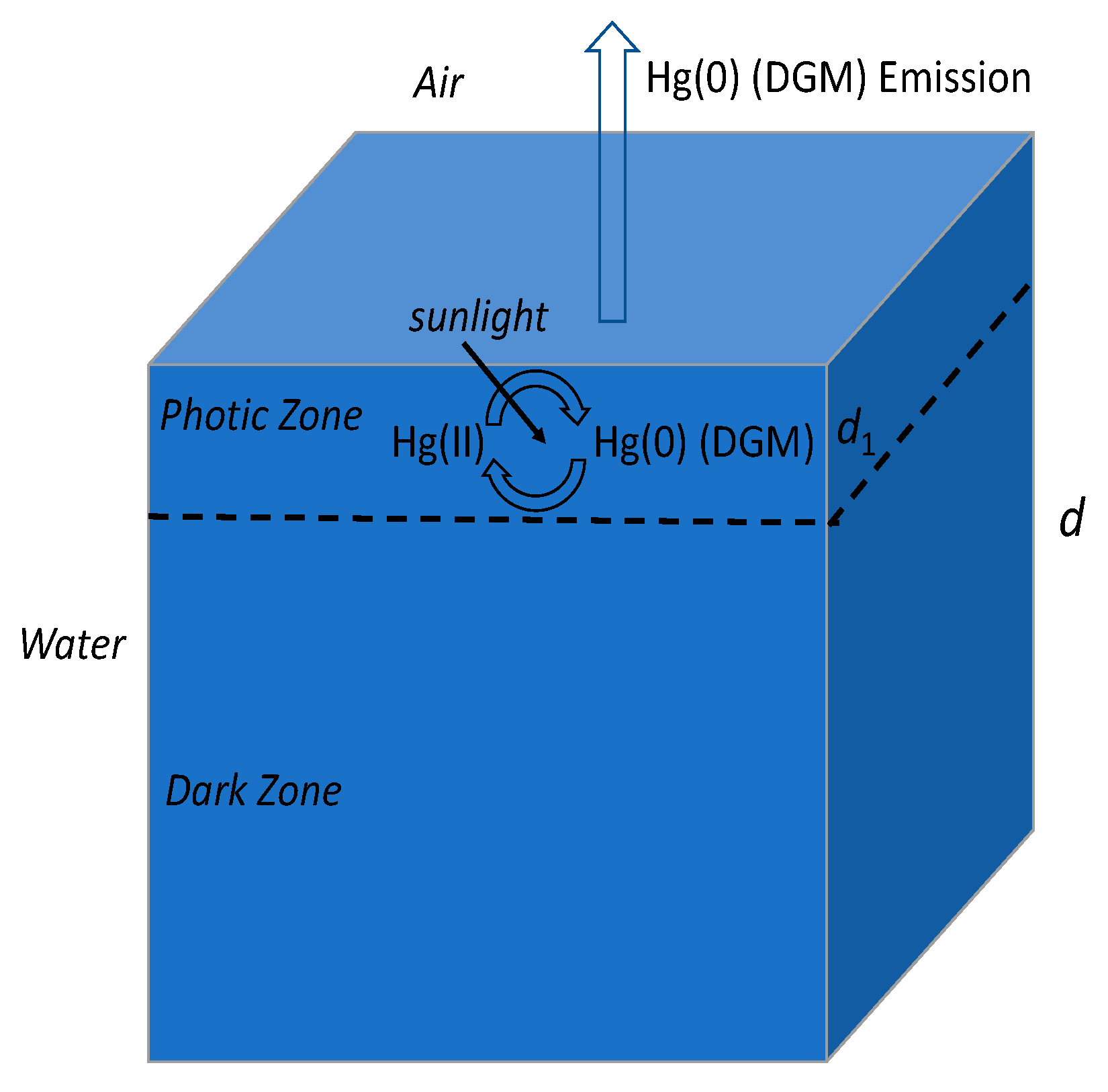
An Arrhenius plot (ln(k_DGM) vs. 1/T) was used to determine whether a relationship between water temperature and the rate constant of the Hg(II) reduction exists. As evident by Figure 3, the rate constant for the Hg(II) reduction is not clearly dependent on the temperature since no clear linear relationship exists between ln(k_DGM) and 1/T. This seems to suggest that the Hg(II) reduction probably is not primarily driven by thermal energy (i.e., the Hg(II) reduction primarily is not a dark reaction) and that the Hg(II) reduction may be more driven by photochemical energy.

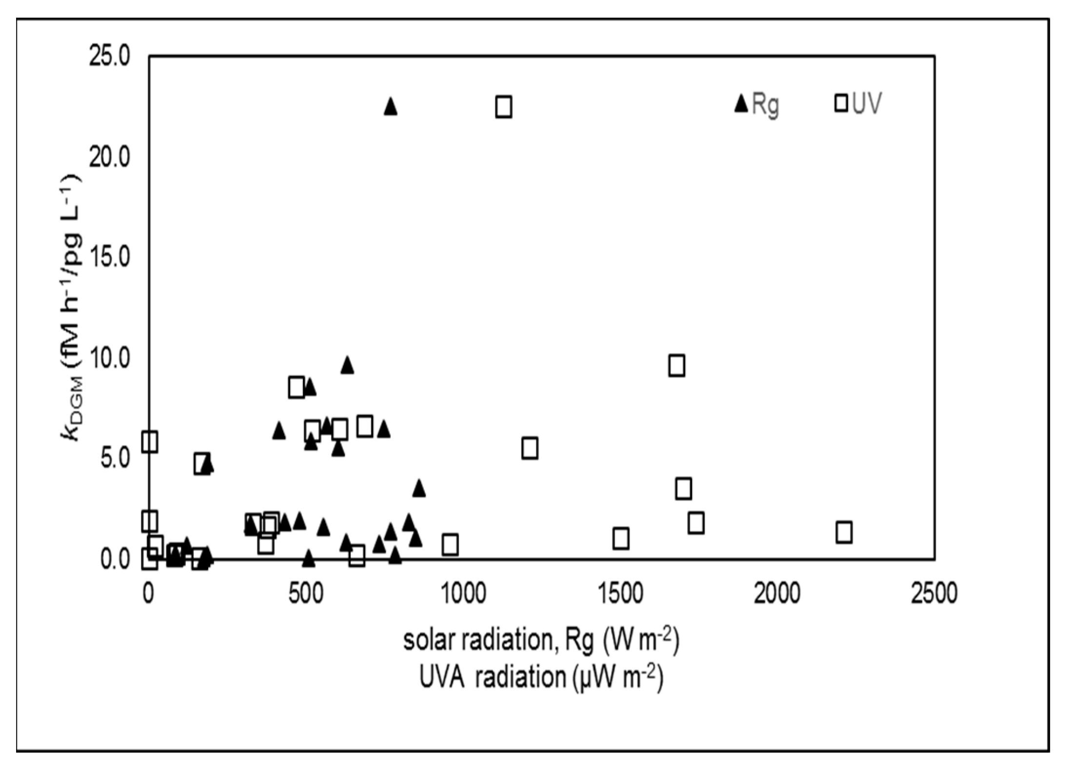
Our examination of the relationship between solar radiation and the rate constant showed no clear distinct trend or correlation (Pearson’s r = 0.2612 for Rg, Pearson’s r = 0.2307 for UVA) for the data pool of the entire calculated rate constants covering both warm and cold seasons (Figure 4). This may stem from a wide variation of solar radiation from all the data available for this model study. A rough trend seems to be quite discernable, however, that higher rate constants correspond to higher solar radiation (Table 1). Moreover, on a seasonal scale, there seems to be a recognizable positive correlation between the daily mean and maximum rate constants and solar radiation (Table 2). These seemingly positive trends lean towards supporting the notion that the Hg(II) reduction is photochemical in its nature. We also examined the Arrhenius plots generated for the data of the cold and warm seasons separately but not found clear or better linear trends (see Chapter 5, [18]).

3.4. Model Sensitivity Study

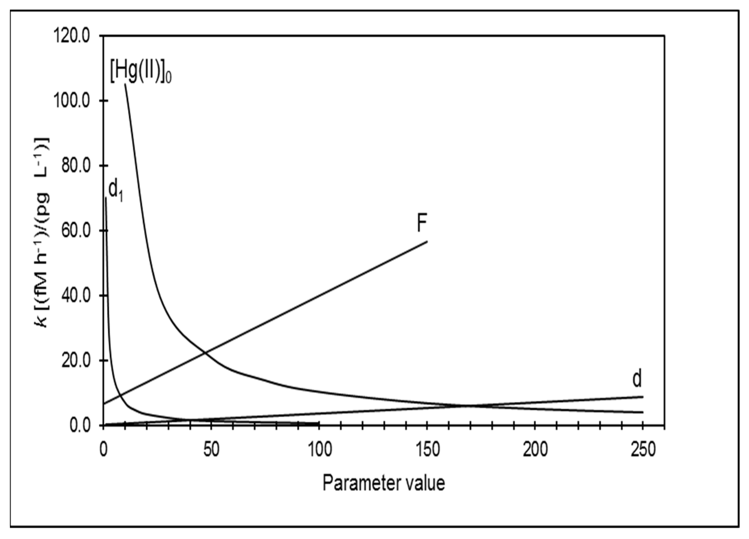
A model sensitivity study was performed by varying one of the model parameters (d, d₁, [Hg(II)]₀, F) with the rest of the parameters fixed to run the model calculations of k_DGM. These calculation results were used to examine the sensitivity of each model parameter tested [18].

The total depth of the water column (d) is a model parameter that defines the size of the water column (the height of the box for the model). A high d value means a deep water column, which leads to more dilution of the surface-generated DGM over the entire box. The depth of the surface photic zone (d₁) is a model parameter that defines the size of the surface space in which solar radiation is readily available, where a high d₁ value leads to a larger surface photic zone. The model parameter [Hg(II)]₀ provides the initial Hg(II) concentration to start the calculation of the kinetic sequence. Hg emission flux (F) is another important model parameter in the model sensitivity study.

When a model sensitivity study was conducted for a particular model parameter, only the value of this parameter was varied while all other parameters were assigned the values as follows (except for the parameter under the sensitivity study): d = 200 cm, d₁ = 10 cm, [Hg(II)]₀ = 150 pg L⁻¹, F = 1 ng m⁻² h⁻¹, ΔDGM = 10 pg L⁻¹, Δt = 1 h.

By inserting the relevant parameters in (6), the following equations were obtained to give a model sensitivity equation for each model parameter:

$$\mathrm{For} d:k_{\mathrm{DGM}}=\frac{1+\frac{10}{d}}{\frac{30}{d}}=\frac{1}{3}+\frac{d}{30}$$

(10)

$$\mathrm{For} d_1:k_{\mathrm{DGM}}= \frac{70}{d_1}$$

(11)

$$\mathrm{For} {[\mathrm{Hg}(\mathrm{II})]}_0:k_{\mathrm{DGM}}=\frac{1050}{{[\mathrm{Hg}(\mathrm{II})]}_0}$$

(12)

$$\mathrm{For} F:k_{\mathrm{DGM}}=\frac{20}{3}+\frac{F}{3}$$

(13)

Figure 5 provides the plots for each of the above model sensitivity equation. Several scenarios of the sensitivity can be recognized as described below.

Scenario 1: at d₁ < 10–15 cm, the depth of photic zone is the most sensitive model parameter, followed by [Hg(II)]₀ and F, with d the least sensitive.

Scenario 2: at [Hg(II)]₀ < 75 pg L⁻¹ and d₁ > 10–15 cm, the initial Hg(II) concentration is the most sensitive model parameter, followed by d₁ and F, with d the least sensitive.

Scenario 3: at [Hg(II)]₀ > 75 pg L⁻¹ and d₁ > 10–15 cm, Hg(0) emission flux (F) is the most sensitive model parameter, followed by [Hg(II)]₀ and d, with d₁ the least sensitive.

The simulation results suggest that the water column depth is generally the least sensitive model parameter. Moreover, Scenario 3 appears to fit in the common conditions of a water system and thus seems to be the most common scenario.

Alternatively, we also carried out the model sensitivity study by using real DGM and Hg(0) emission flux data paired in the real time periods inserted into the sensitivity calculation equations. The detailed results are provided elsewhere (see Chapter 5, [18]). Generally, the results of this alternative model sensitivity study appear to be similar to what have been described as above as shown in Figure 5.

Incidentally, the model sensitivity study (the model sensitivity Equations (10)–(13)) can also provide a means to find the rate constants under other conditions in which the model parameters have other values than those used in the model calculations as reported in this paper.

4. Conclusions

This model study generated useful and valuable results and interesting findings. The major conclusions that can be drawn from this study are as follows:

• The rate constants of the Hg(II) photoreduction calculated from our model are comparable to in order of magnitude but consistently higher, especially for the warm season, than and thus deviate from the published rate constants in the literature from various other field and laboratory studies. The model calculated rates of DGM production are one order of magnitude higher (10² vs. 10¹) than the calculated apparent rates solely using the DGM data without considering the Hg emission. These results jointly provide strong evidences to suggest that the omission of DGM emission can lead to an underestimation of the rate constants and therefore the rates as well.
• The model sensitivity analysis suggests that the most sensitive model parameter in the mass balance box model, under ordinary environmental conditions, is the DGM evasion flux. This again supports the notion that the flux is a key parameter needed for determining the real kinetics of aquatic Hg(II) photoreduction.
• This model study demonstrates that the model calculation can provide an alternative, independent, valuable estimation of aquatic Hg photoreduction kinetics. The model approach is thus a useful means of estimating the kinetics of aquatic Hg(II) photoreduction with consideration of DGM emission from the water systems.
• There seems no clear seasonal correlation between solar or UVA radiation and the model-calculated rate constants of the Hg(II) photoreduction, although UVA radiation appears to have an impact on the Hg(II) photoreduction as shown by some of our daily results. Further investigation with expanded field data should be valuable.