
Investigation on Stall Characteristics of Centrifugal Pump with Guide Vanes

1
College of Energy and Electrical Engineering, Hohai University, Nanjing 211100, China
2
Beijing Aerospace Propulsion Institute, China Aerospace Science and Technology Corporation, Beijing 100176, China
3
National Marine Hazard Mitigation Service, Beijing 100194, China
4
Key Laboratory of Fluid and Power Machinery of Ministry of Education, Xihua University, Chengdu 610039, China
*
Author to whom correspondence should be addressed.
Water 2023, 15(1), 21; https://doi.org/10.3390/w15010021
Submission received: 8 December 2022
/
Revised: 17 December 2022
/
Accepted: 19 December 2022
/
Published: 21 December 2022
(This article belongs to the Special Issue Advances in Hydrodynamics of Water Pump Station System)
Abstract
:Stall usually occurs in the hump area of the head curve, which will block the channel and aggravate the pump vibration. For centrifugal pumps with guide vanes usually have a clocking effect, the stall characteristic at different clocking positions should be focused. In this paper, the flow field of the centrifugal pump under stall conditions is numerically simulated, and the rotor–stator interaction effects of the centrifugal pump under stall conditions are studied. The double-hump characteristic is found in the head curve by using SAS (Scale Adaptive Simulation) model. The hump area close to the optimal working condition is caused by hydraulic loss, while the hump area far away from the optimal working condition point is caused by the combined action of Euler’s head and hydraulic loss. The SAS model can accurately calculate the wall friction loss, thus predicting the double-hump phenomenon. The pressure fluctuation and head characteristics at different clocking positions under stall conditions are obtained. It is found that when the guide vanes outlet in line with the volute tongue, the corresponding head is the highest, and the pressure fluctuation is the lowest. The mechanism of the clocking effect in the centrifugal pump with guide vanes is obtained by simplifying the hydrofoil. It is found that when the downstream hydrofoil leading edge is always interfered with by the upstream hydrofoil wake, the wake with low energy mixes the boundary layer with low energy, which causes small-pressure pulsation. The results could be used for the operation of centrifugal pumps with guide vanes.
1. Introduction
The stall of a centrifugal pump is an unstable flow phenomenon when it operates at low flow rate [1,2,3,4]. The stall phenomenon was first discovered by Stenning in a centrifugal compressor test [5], and in-depth research was carried out in this field [6,7]. In the mid-1980s, the stall problem in centrifugal pumps began to receive widespread attention [8]. Centrifugal pumps often suffer from severe pressure pulsations when operating under stall conditions, which further aggravates the vibration and noise of the pump and, in severe cases, causes fatigue damage to the blades [9,10]. Especially in recent years, with the continuous construction of large pump stations, higher requirements have been put forward for the safe and stable operation of pumps, so it is of great significance to understand the stall problem and then control it.
CFD is an important way to reveal the internal flow mechanism [11,12]. For the stall of centrifugal pumps, accurate prediction of stall phenomenon is the basis of research. The stall of centrifugal pumps is a complex rotational separated flow. At present, the calculation of three-dimensional separated flow mainly includes Reynolds average method (RANS), large eddy simulation method (LES), and mixed URANS/LES method [13]. Among them, LES model can analyze the turbulent vortex structure, turbulence fluctuation, and other information of complex flow in more detail, but it is difficult to apply to the calculation of existing engineering problems due to its huge amount of calculation [14]. At present, RANS and URANS/LES methods are the most commonly used methods. The stall in the guide vane is calculated by the standard k-ε model [15], but there is a large difference between the experimental data and the simulated data. Braun [16] used the SST k-ω model to simulate a pump and found the model can predict the phenomenon of rotating stall, but the flow at the stall point and the propagation speed of the stall cell are larger than those in the test. Lucius [17] and Zhang [18] adopted the URANS/LES model to calculate a centrifugal pump that was tested at Magdeburg University in Germany. It was found that the predicted head and rotating stall vortex frequency were close with experiment, but the predicted peak values were different. Therefore, it is necessary to select turbulence models according to specific problems.
Many scholars have carried out a great deal of research on the factors affecting the stall of centrifugal pumps. The main influencing factors are pump flow [19,20,21,22,23], impeller speed [24,25,26], number of blades [27,28], and rotor–stator interaction [29,30,31]. For the guide-vane centrifugal pump, the clocking position of the guide vane is also an important factor affecting the internal flow characteristics of the centrifugal pump. Clocking effect refers to the influence of changing the circumferential relative position between the blades on turbomachinery [32]. Benigni [33] and Wang [34,35] studied the clocking effect of an annular volute centrifugal pump. The results show that the clocking effect has a greater impact on the pressure fluctuation in the pump, especially on the pressure fluctuation intensity of the volute. Tan [36] studied the clocking effect of the high head multistage centrifugal pump and found that the clocking effect had a significant impact on the internal pressure and radial force of the pump. However, the influence of clocking effect on the internal flow characteristics of centrifugal pumps at stall conditions is rarely reported.
In this paper, the turbulence models are compared and analyzed in order to accurately predict the flow characteristics in the pump, and then, the influence of the clocking effect on the pump flow at stall conditions is further analyzed. Meanwhile, due to the complex structure of the centrifugal pump, in order to better explore the clocking effect of the guide-vane centrifugal pump, this paper establishes a simplified model based on the structural characteristics of the rotor and stator in the centrifugal pump in order to deeply analyze the mechanism of clocking effect in the centrifugal pump.
2. Research Object and Numerical Calculation Method
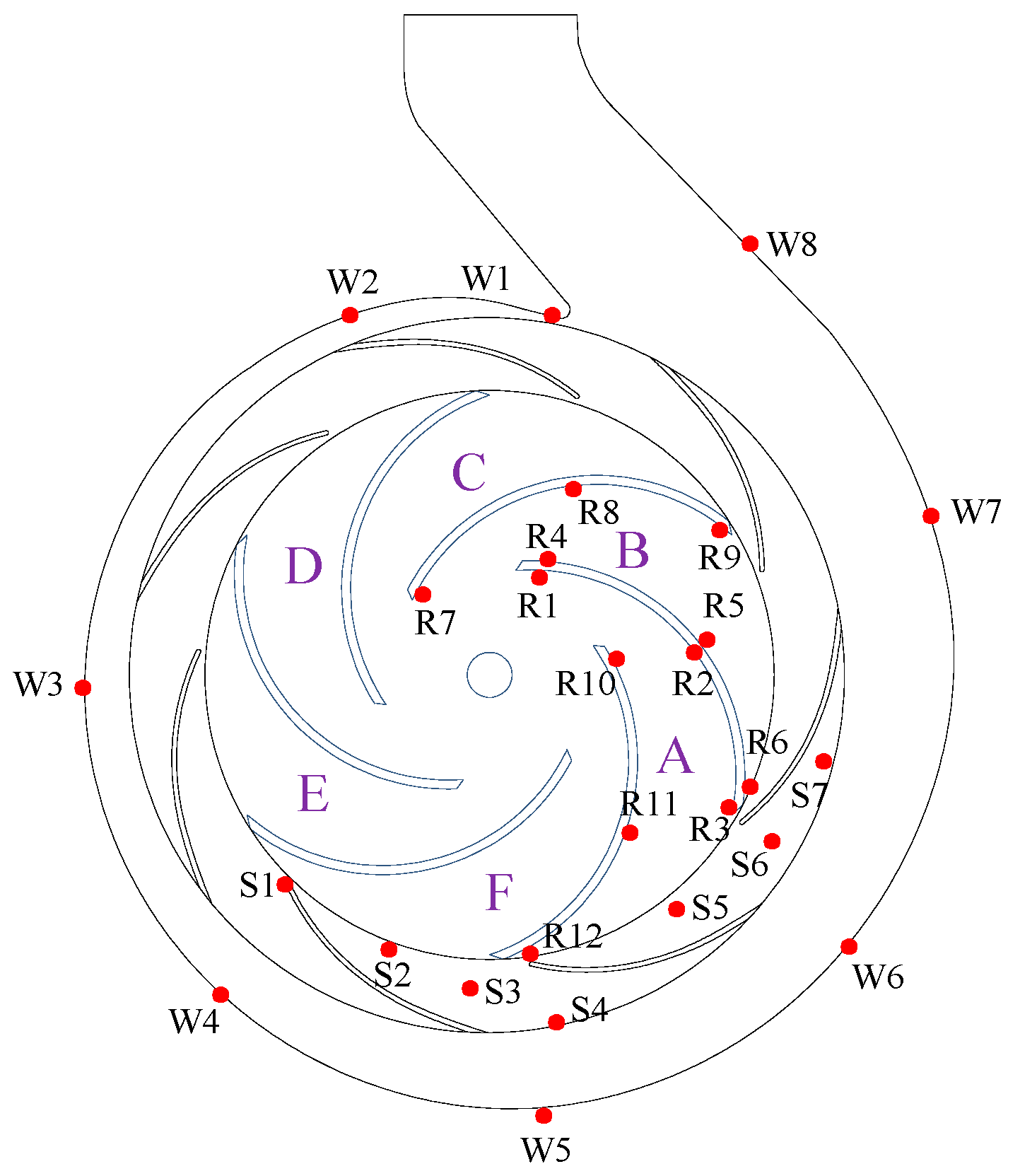
The geometric structure of the centrifugal pump with guide vane selected as the calculation object in this paper is shown in Figure 1. Combined with the internal flow structure of the pump, the pressure fluctuations in the guide vane and impeller regions are analyzed, respectively. Figure 1 is the axial sectional view of the guide vane centrifugal pump. The six flow channels are named A-F. Three monitoring points are set on the pressure surface and suction surface of the blades in the two flow channels of the impeller along the direction from the inlet to the outlet. Similarly, three monitoring points are set in two adjacent flow channels of the guide vane. During the calculation, the pressure fluctuation of these points is recorded with time.
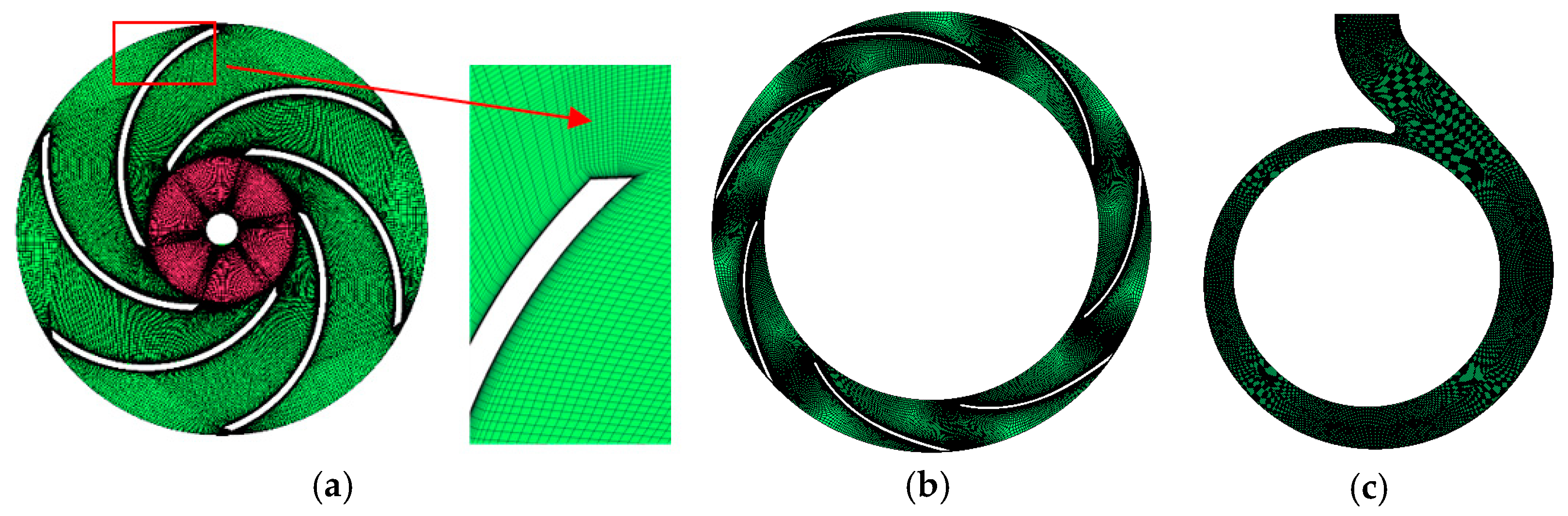
The hexahedral structure grid is used to divide the computational domain. With the purpose of ensuring the reliability of the calculation, taking the near-wall grid into account is necessary. To do this, the first layer of the grid is validated. After testing, y + < 30, which means the mesh is suitable for turbulence models, as shown in Figure 2. In order to verify the independence of grid, different grid amounts are calculated in the rated condition. The pump head is selected as the target parameter for grid independence verification, and its variation with the number of grids is observed. The number of grids is added at the tongue region of volute and blade surface. The calculation domain with different grid numbers is simulated by applying the SST k-ω turbulence model. The head rises when grids elements increase from 2.34 million to 4.17 million. The variation of heads is scarce when grid elements increase to 5.27 million. In conclusion, the elements of grids make a small difference in the results when they continue to increase. Therefore, the elements of grids of the pump will be controlled at about 5.27 million, and the corresponding number of nodes is 4.1 million.
The velocity inlet and pressure outlet are adopted. The rotor–stator interface adopts the transient frozen rotor technology, and the impeller speed is set as 725 r/min to keep consistent with the test. The no-slip condition is adopted in the wall boundary. The governing equations are discretized by the finite volume method in space and the second-order implicit scheme in the time domain. The time step is 2.3 × 10⁻⁴ s, which is 1/360 of the rotation period. The convergence residual is set to 1.0 × 10⁻⁵. This calculation is carried out on the rack server of Hohai University. The servers all use 64-bit high-performance processors and 12 dual computing nodes, including 24 Intel E5-2600 eight-core processors and 192 CPU cores. Each node contains 64 GB of memory, and the total system memory is 678 GB.
When the centrifugal pump impeller stall occurs, the particularity and complexity of the internal flow put forward higher requirements for the numerical simulation method. The numerical results calculated by the SST k-ω and SAS model are compared.
The turbulent kinetic energy and dissipation rate in the SST k-ω model can be expressed as follows [37]:
This model has become the standard in many industrial applications. The coefficients in the formulas are given in reference [38].
The “scale-adaptive” feature of SAS model is mainly embodied in its definition of a second order velocity ladder [39]. Many scholars have applied the model in the simulation of rotating machinery and proved the reliability of the model. The construction method of the SAS model is based on the SST model by adding the source term QSAS to the ω equation:
The coefficients in the formulas are given in reference [39].
3. Prediction of Centrifugal Pump Performance Curve
The internal flow of the centrifugal pump with guide vanes is complex. In order to systematically analyze the internal stall flow characteristics of the pump, the full operating ranges are calculated. The research object of this paper is the experimental centrifugal pump of Technical University of Denmark (DTU). In the experiment, PIV and LDV methods are used to collect the data of single-stage impeller so as to obtain the information on average flow field. The impeller inlet flow is changed by adjusting the diameter of the hole on the resistance plate. The adjustment range is (15–100%) Qd, where Qd is the flow under design conditions. In order to stabilize the flow field at the pump inlet, a rectifier is placed in the pipe section at the inlet of the resistance plate and impeller [40].
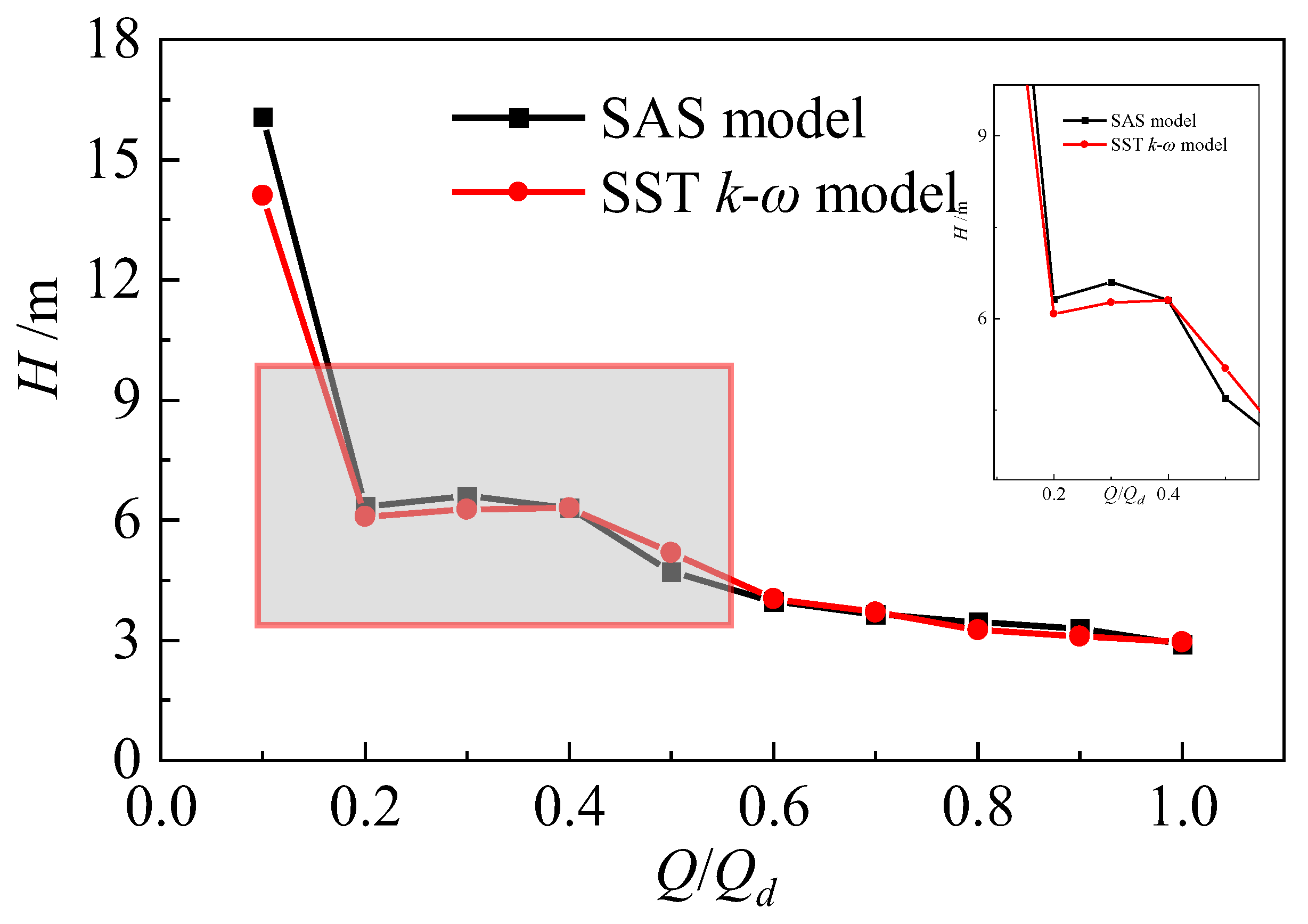
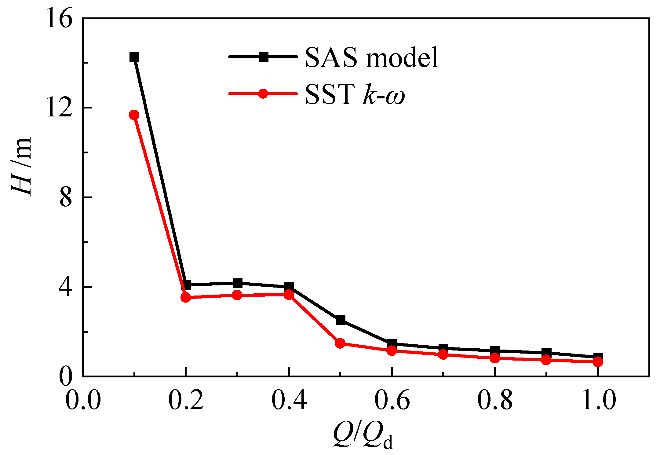
The comparison results of the numerical simulation of centrifugal pumps at different working conditions are shown in Figure 3. The head of centrifugal pumps without guide vanes calculated by the two models are close to the experimental values, indicating that the numerical model method can accurately predict the energy characteristics of centrifugal pumps. In the guide-vane centrifugal pump, the existence of the guide vane increases the mechanical loss and changes the head. In terms of head prediction performance, the two models both predict the hump area at 0.2 Qd–0.3 Qd, in which the hump peak point is 0.3 Qd, and the wave trough is 0.2 Qd. The difference is that the SAS model observed the occurrence of the hump phenomenon at 0.5 Qd–0.6 Qd, in which the peak point is 0.6 Qd, and the wave trough point is 0.5 Qd. The double-hump phenomenon of guide vane centrifugal pump predicted by the SAS model is also observed in the pump turbine [41].
4. Characteristic Analysis of Double Humps
Through the numerical simulation analysis in the previous section, the guide vane centrifugal pump has a double-hump characteristic, and the emergence of the hump area must be accompanied by the unstable flow. In order to further analyze the causes of this phenomenon, this section focuses on the hydraulic loss of each component.
The head characteristic of the guide-vane centrifugal pump is caused by the combined action of Euler head and hydraulic losses of flow passage components. Euler energy (ΔCu·U) is the difference between impeller outlet velocity moment (Cu2·U2) and impeller inlet velocity moment (Cu1·U1). In the process of numerical simulation, Euler energy and Euler head can be obtained through equations [41]:
Figure 4 shows the results of Euler head calculated by the two models. It can be seen that the Euler head factor increases with the decrease of flow rates. In the Euler head calculated by SAS, when the flow rate changes from 1.0 Qd to 0.5 Qd, the Euler head decreases slowly; when the flow decreases from 0.5 Qd to 0.4 Qd, the Euler head decreases rapidly. For the Euler head calculated by SST k-ω, when the flow rate changes from 1.0 Qd to 0.6 Qd, the Euler head decreases slowly; when the flow decreases from 0.6 Qd to 0.5 Qd, the Euler head decreases rapidly. The hump area is observed at 0.2 Qd–0.3 Qd of Euler head calculated by the two models, where the peak point is 0.3 Qd, and the trough is 0.2 Qd.
In the hydraulic loss analysis of flow passage components, the loss size of a section of the area can be obtained through the traditional differential pressure analysis method. Figure 5 shows the calculation of the total head loss of the guide-vane centrifugal pump in the full flow channel. In the Euler head calculated by the SAS model, when the flow changes from 1.0 Qd, to 0.6 Qd, the head loss decreases slowly; when the flow decreases from 0.6 Qd, to 0.5 Qd, the hydraulic loss increases rapidly. For the Euler head calculated by SST k-ω, when the flow rate changes from 1.0 Qd to 0.5 Qd, the Euler head decreases slowly; when the flow decreases from 0.5 Qd, to 0.4 Qd, the hydraulic loss increases rapidly. Under each working condition, the hydraulic loss calculated by SAS model is greater than SST k-ω. Due to the entropy, generation of the wall area is calculated more accurately by the SAS model, so the hydraulic loss obtained is greater than SST k-ω.
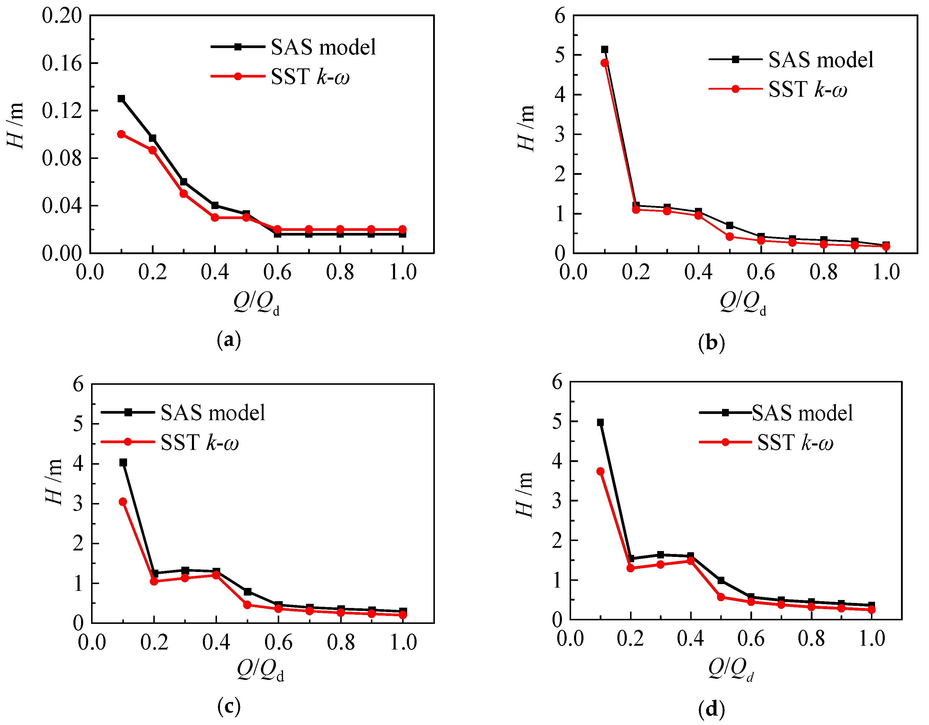
Figure 6 shows the head loss calculation of each component under different flow rates. The hydraulic loss of each component is the minimum at the design condition. Hydraulic loss of guide-vane centrifugal pump mainly comes from guide vane and impeller. For the hydraulic loss calculated by the SAS model, the head curve corresponds to the 0.5 Qd–0.6 Qd hump area close to the design working condition. From the peak point (0.6 Qd) to the trough point (0.5 Qd) in the hump area, the hydraulic loss of each component suddenly increases, in which the impeller and guide vane increase greatly, while the corresponding Euler head changes little. Therefore, the hump here is mainly caused by hydraulic loss. During the 0.5 Qd–0.6 Qd operating condition, there is no hump area calculated by the SST k-ω model because the hydraulic loss of components does not change much. When the flow rates decrease from 0.5 Qd to 0.4 Qd, the hydraulic loss increases rapidly, but the calculated Euler head increases at this time, offsetting the occurrence of the hump area. In the hump area of 0.2 Qd–0.3 Qd, the Euler head calculated by the two models decreases, and the hydraulic loss increases. Therefore, the hump area is the result of the joint action of Euler head and hydraulic loss.
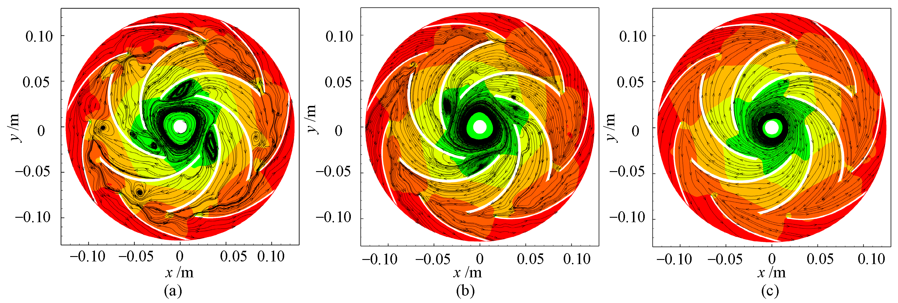
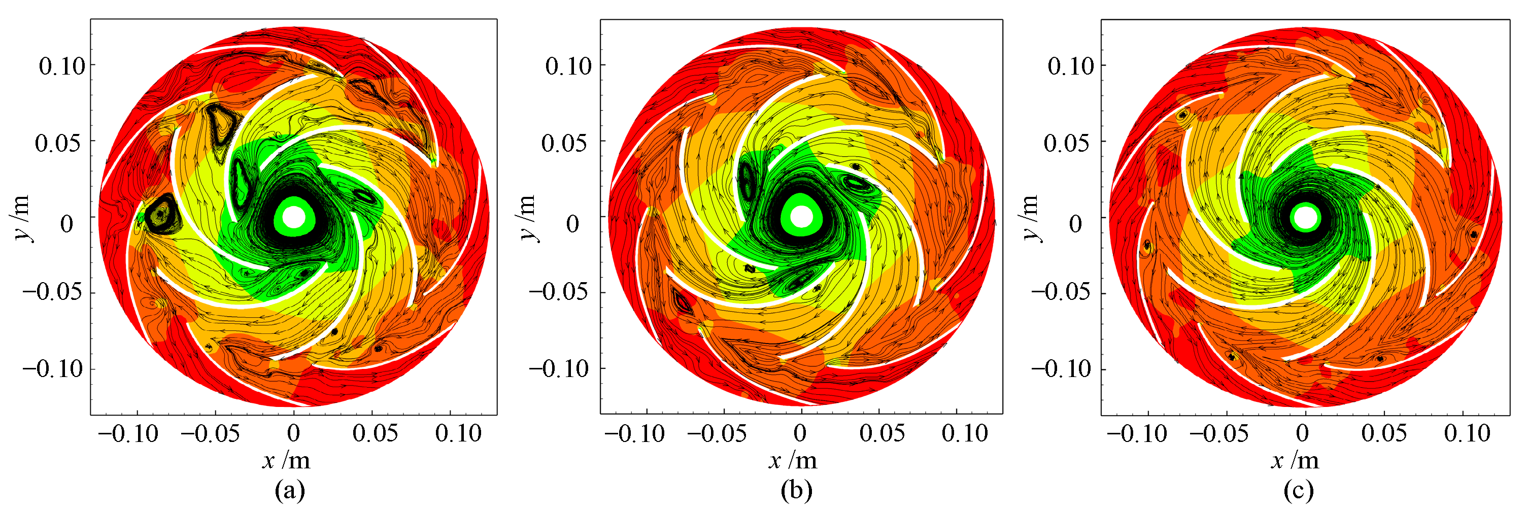
As shown in Figure 7 and Figure 8, the flow patterns inside the impeller at different working conditions are compared. At different working conditions, the influence of the guide vane on the internal flow of the impeller is different. At 0.7 Qd, the stall passage of the impeller calculated by the two models does not change much. However, in the guide-vane passage, a separation vortex at the back of the guide vane is observed in the flow field calculated by the SAS model, which indicates that the loss of the guide vane begins to increase at this time. At 0.5 Qd, the stall vortex is obvious in the impeller calculated by the two models. There are relatively large stall cells calculated by the SST k-ω model in channels A, C, and E, and they are all located on the suction surface of the impeller blade head and in the middle of the impeller pressure surface. There are also stall cells calculated by the SAS model in the flow channels in A, C, and E channels, which is similar to SST k-ω. The difference is that the previous two small vortices become a larger one, which is located near the suction surface of the impeller inlet, and the size of the stall cells almost blocks the entire flow passage. At 0.3 Qd, the flow pattern of the impeller calculated by the two models becomes worse. From the results calculated by SST k-ω, the relatively large stall vortices are observed in channels A, C, and E, while the flow in the other three channels is relatively stable. Stall cells appear in all six channels from the results calculated by the SAS model, which is consistent with the phenomenon observed in the external characteristic curve in Figure 3. When the pump operates at 0.3 Qd, the head curve is at the trough of the wave, which indicates that the hump in the head flow curve is largely caused by the stall in the impeller flow passage.
5. Clocking Effect of Guide-Vane Centrifugal Pump under Stall Characteristics
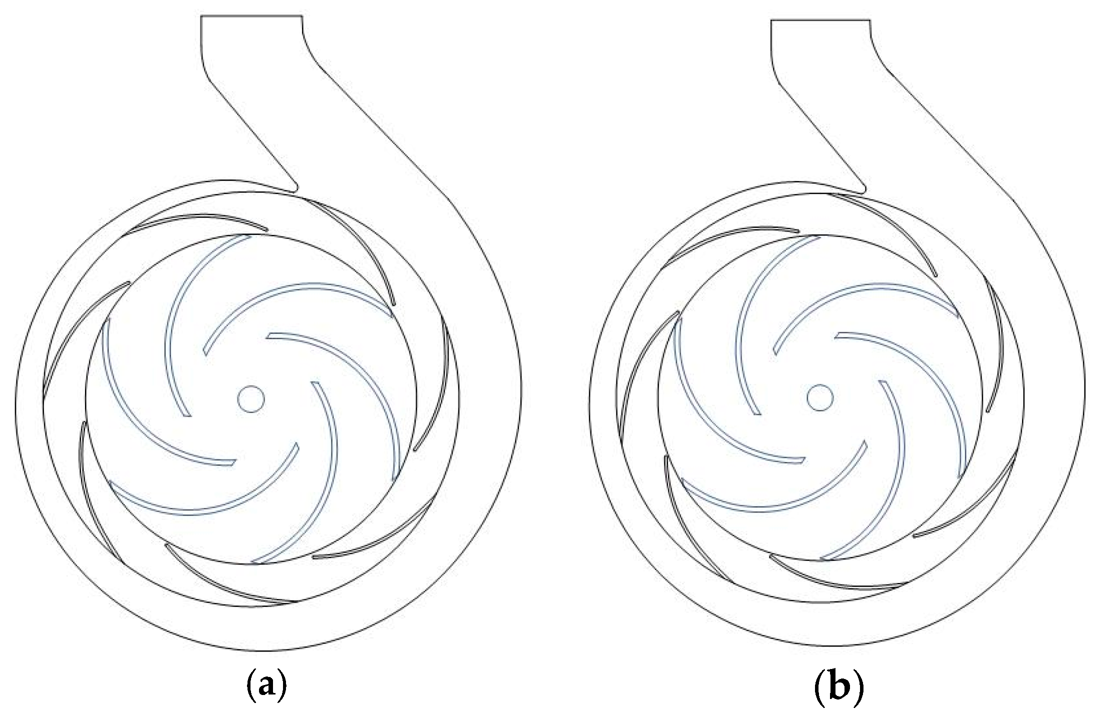
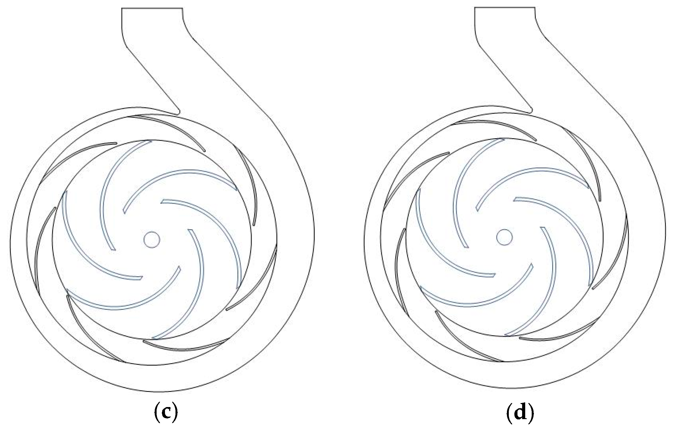
Figure 9 shows the general assembly drawing of the centrifugal pump with a guide vane. In order to study the influence of the clocking position of the guide vane on the pump performance and the pressure fluctuation on the volute wall, four guide-vane installation positions are selected by rotating the guide vane, as shown in Figure 9. The guide-vane positions 2, 3, and 4 are obtained by rotating the guide-vane position 1 clockwise by 12.5°. The included angle between two adjacent vanes of the guide vane is 51.43°. For clocking position 1, the guide vanes outlet in line with the volute tongue. For clocking positions 2, 3, and 4, the position of the guide-vane outlet and volute tongue are staggered by 12.5°, 25°, and 37.5°, respectively.
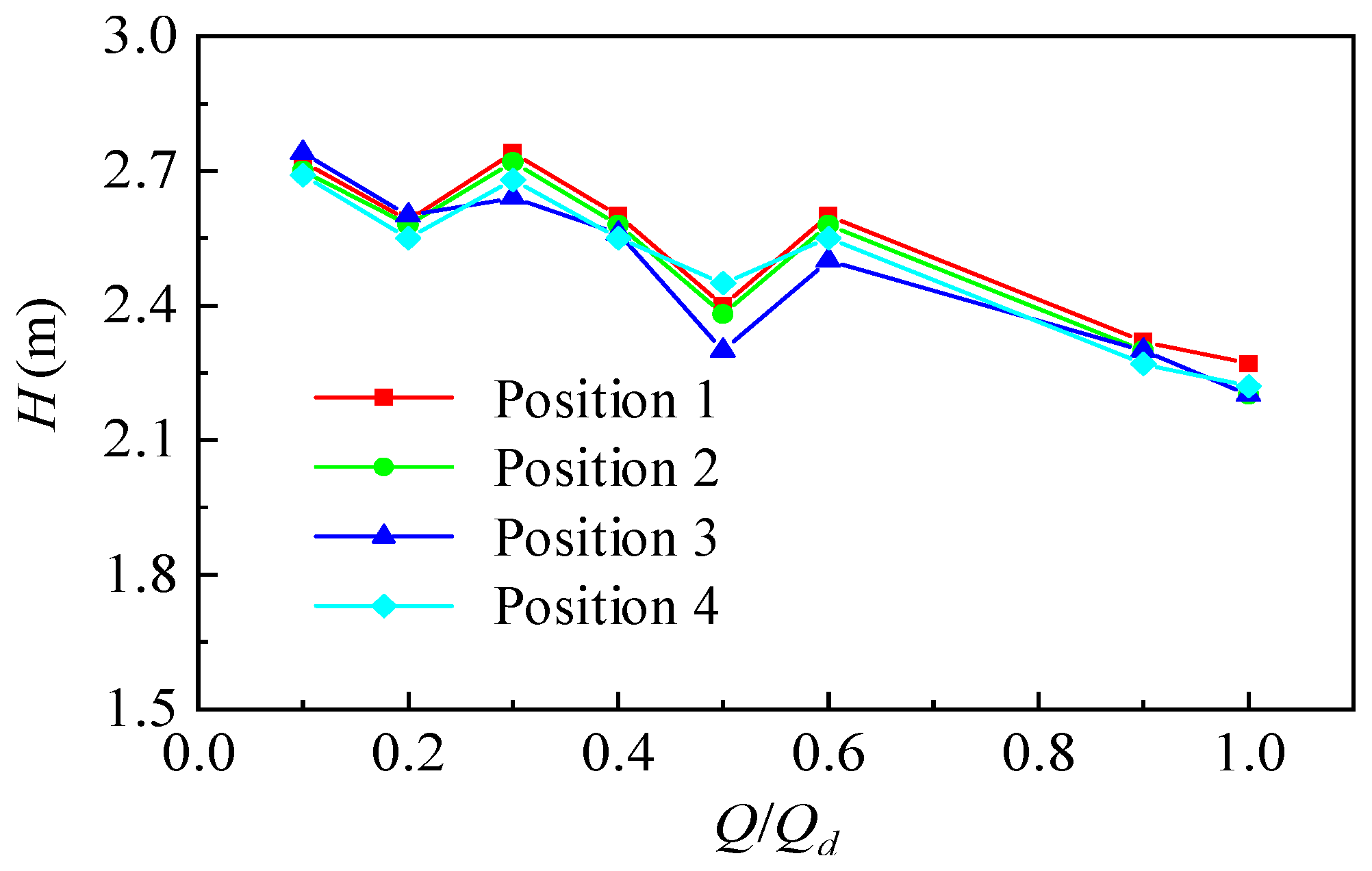
The head curve of the centrifugal pump with guide vanes at four clocking positions is compared, as shown in Figure 10. When the guide vane is installed at clocking position 1, the head is maximum at large flow rate conditions. When the guide vane is installed at clocking position 3, the head is the minimum at all flow rate conditions. Different clocking positions have a great impact on pump performance at low flow rate conditions, and the maximum head difference is 0.5 m. The double humps occur at all four clocking positions, and the humps are observed at 0.2 Qd–0.3 Qd and 0.5 Qd–0.6 Qd.
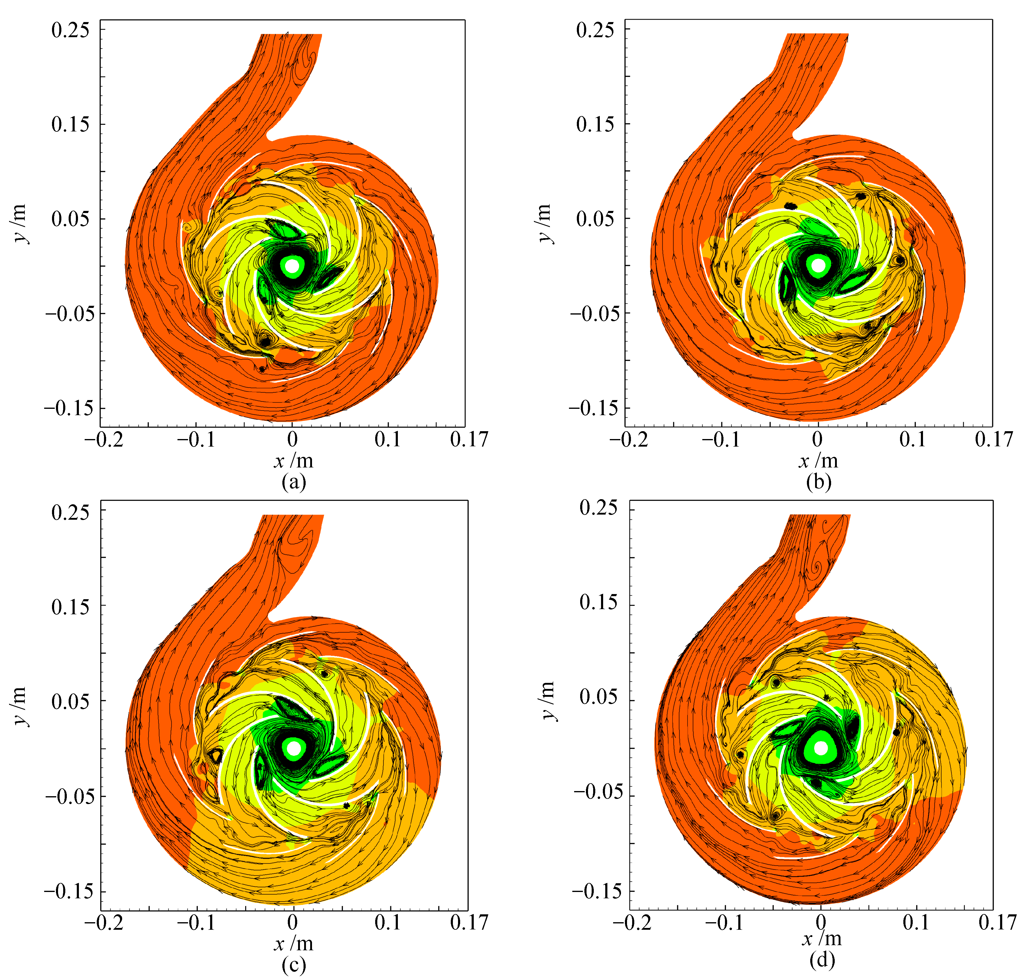
The comparison of the streamline distribution at four clocking positions at 0.3 Qd is shown in Figure 11. The clocking position has a great influence on the flow structure of the guide vane, and different sizes of reflux areas are generated in the flow passage, which is due to the flow separation occurring at the pressure side of the guide vane. Meanwhile, part of the fluid in the guide-vane flow passage flows out of the volute outlet, and part of the fluid enters the volute flow passage. In addition, the velocity direction on the right side of the volute outlet and the vortex structure on the left side is obviously affected by the guide-vane position. In the head curve, the head difference is large at 0.3 Qd because the flow structure at the outlet of the guide vane close to the volute outlet is greatly affected by the position of the guide vane, which results in flow separation at the volute outlet, causing hydraulic loss.
Figure 12 shows the pressure fluctuation of monitoring points in the impeller and guide vane at 0.3 Qd. In the middle of the impeller, Figure 12a shows that the guide-vane position at stall condition has a significant impact on the instability characteristics of pressure fluctuation caused by rotor–stator interaction. When the guide vane is installed at position 1, the amplitude of the blade is at a relatively stable minimum; when the guide vane is at position 3, the pressure fluctuation amplitude of the blade has strong instability, which is greatly affected by the rotating position of the impeller. Due to the existence of the vortex at the inlet of the blade suction side, the pressure fluctuation amplitude is enhanced, and the peak-to-peak value is large. In the vaneless region, which is the gap between the impeller and the guide vanes, the flow interference is strong, and the pressure fluctuation signals are relatively greater, and the peak-to-peak value of the pressure fluctuation is the largest. Therefore, when the stall cell moves to the monitoring point, the pressure decreases rapidly, and after the stall cell falls off, the pressure value rises again. Stall cells periodically form, develop, and fall off, inducing low-frequency pressure fluctuations.
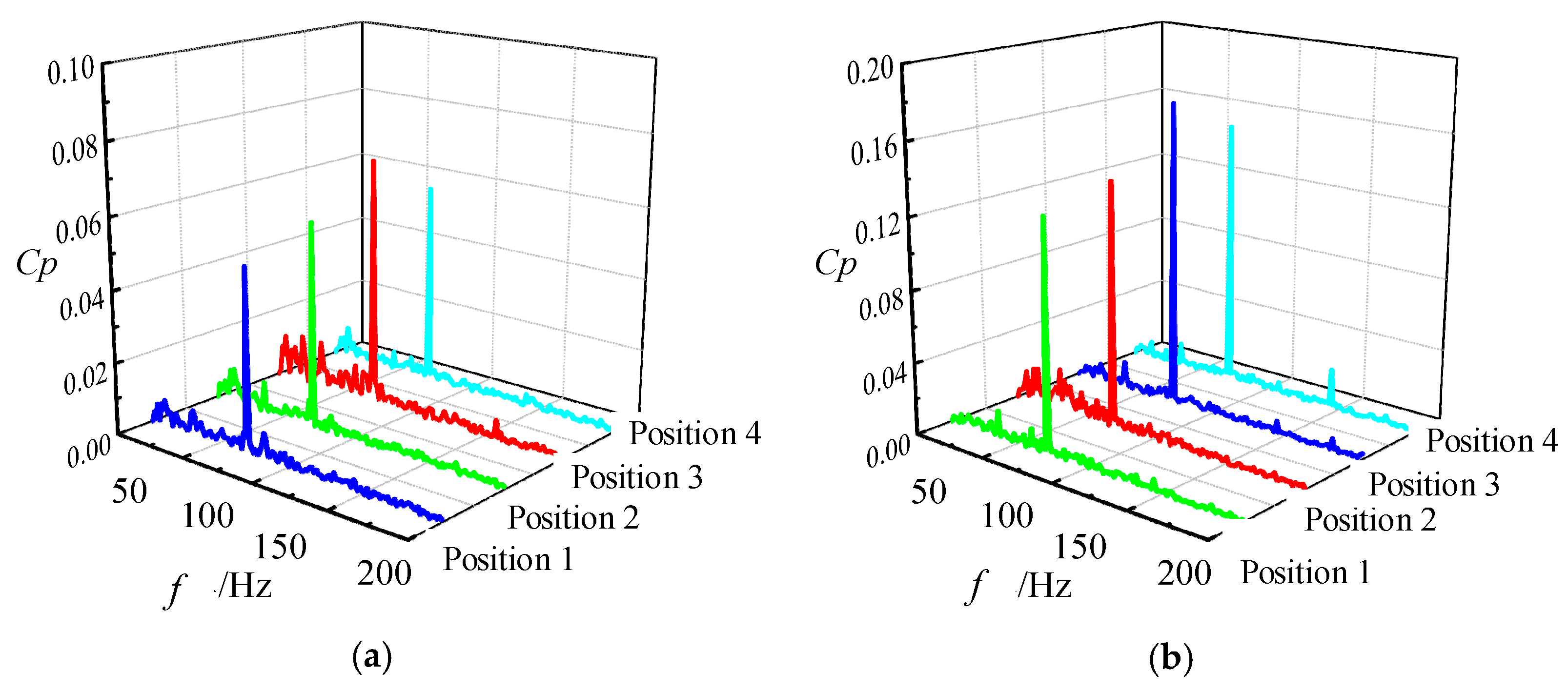
Figure 13 shows the pressure fluctuation of the volute at 0.3 Qd. The clocking position of the guide vane has a significant impact on the dominant frequency and corresponding amplitude of the volute. In the four clocking positions, the dominant frequency at the volute tongue is blade frequency (75 Hz), and the secondary frequency is low frequency. When the guide vane is installed at clocking position 1, the fluctuation amplitude of the dominant frequency is maximum, and when it is installed at clocking position 3, the fluctuation amplitude of the dominant frequency is minimum. The amplitude of dominant frequency fluctuation at clocking position 3 is 1.3 times of that at clocking position 1. At the outlet of the volute, one time of the dominant frequency corresponding to clocking position 1 is the blade frequency (75 Hz), and the dominant frequency at other clocking positions is the low frequency. From Figure 11, it can be seen that the streamline at clocking positions 2, 3, and 4 is twisted at the outlet of the volute, while the streamline at the outlet corresponding to timing position 1 is relatively smooth. Therefore, the timing position affects the flow at the outlet of the volute so that the volute will produce a low-frequency fluctuation.
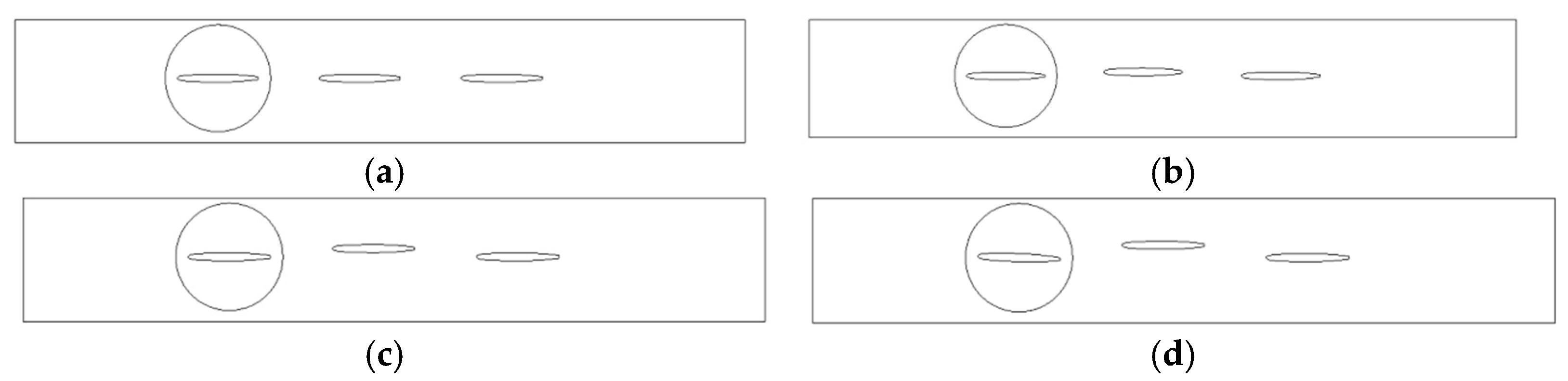
In order to further study the clocking effect, the guide vane and volute tongue are simplified as two static hydrofoils [42]. The flow is controlled by the upstream valve angle for hydraulic characteristics research at different operating conditions. The clocking position is changed by changing the vertical position of the first hydrofoil, as shown in Figure 14.
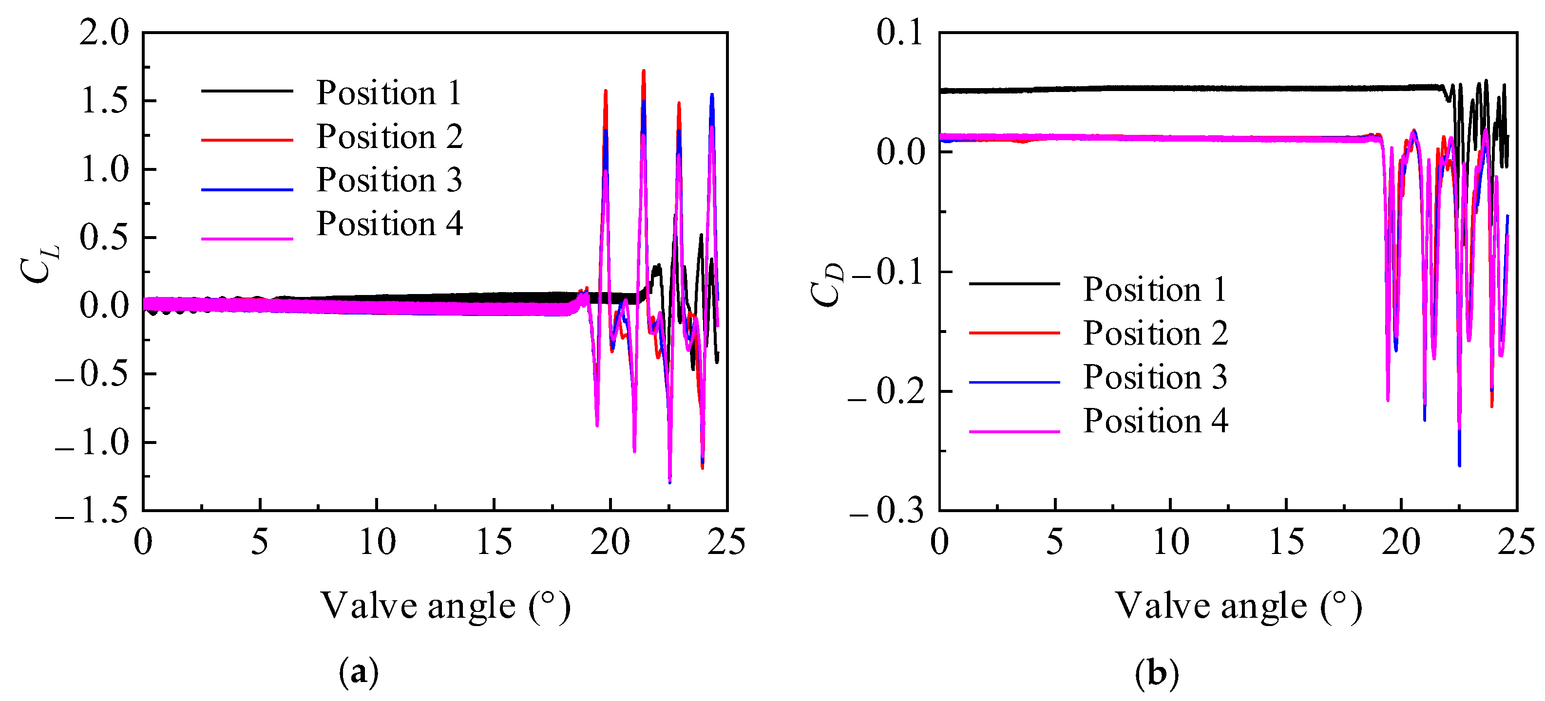
Figure 15 shows the change of lift and drag coefficient of the secondary hydrofoil. It can be seen that with the decrease of flow rate, the secondary hydrofoil at the four clocking positions shows the characteristics of first stabilization and then oscillation. The difference is that at clocking position 1, the secondary hydrofoil starts to oscillate at a lower flow rate, and the amplitude of oscillation is much smaller than that at the other three positions.
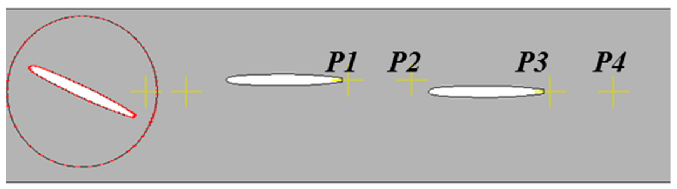
Figure 16 shows the arrangement of pressure fluctuation measuring points. The monitoring points, P1~P4, are arranged at different positions upstream and downstream of the secondary hydrofoil center. P1 and P2 are located at 0.1 L and 0.5 L at the tail of the first hydrofoil, and P3 and P4 are located at 0.1 L and 0.5 L at the tail of the second hydrofoil.
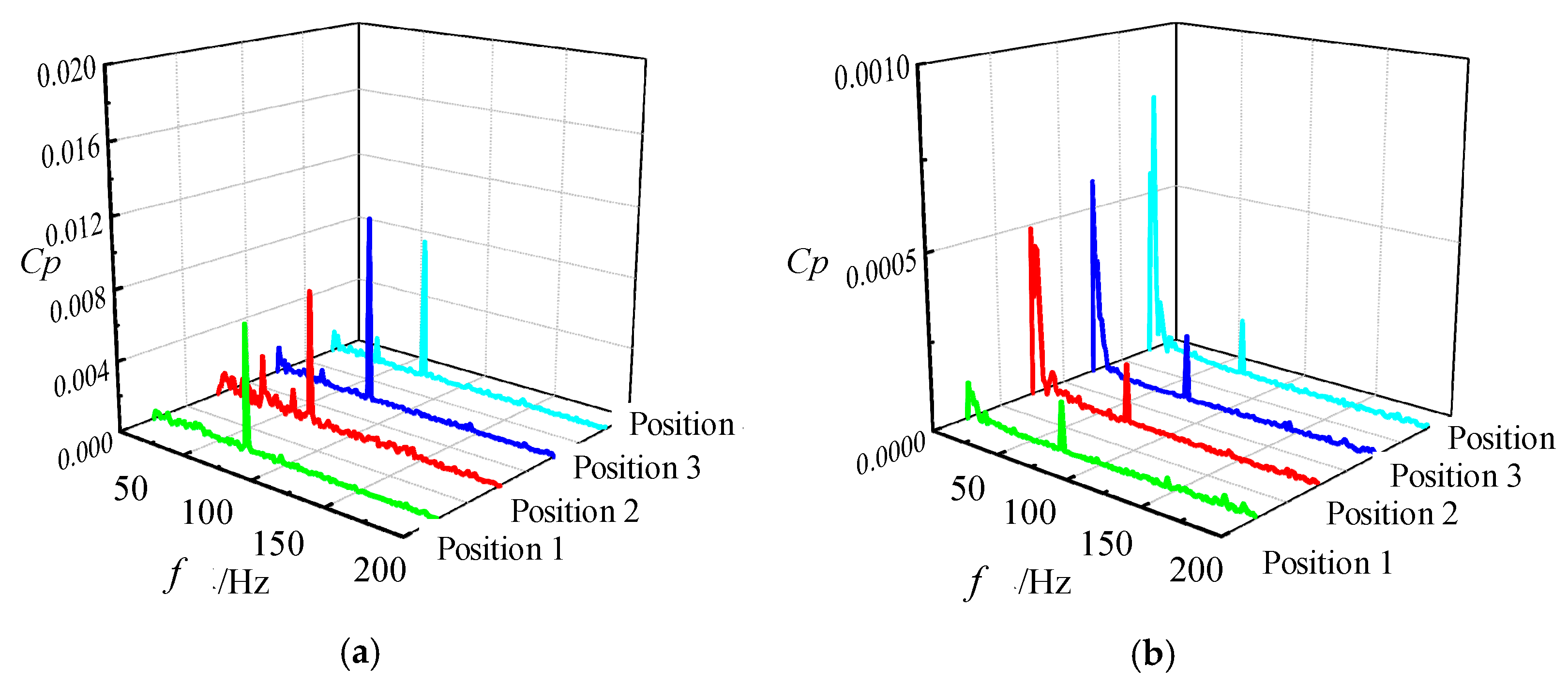
Figure 17 shows the pressure distribution of different monitoring points. It can be seen from the figure that for the monitoring points P1 and P2 at upstream of the secondary hydrofoil, the pressure changes with time tend to stabilize first and then increase. The pressure changes at the four clocking positions are 20°, 19°, 18°, and 17°, respectively. With the continuous rotation of the valve plate, the clearance between the valve plate and the pipe wall gradually changes, the flow rate decreases, and the pressure increases. Among the four clocking positions, the pressure fluctuation range of clocking position 1 is obviously smaller than that of other clocking positions.
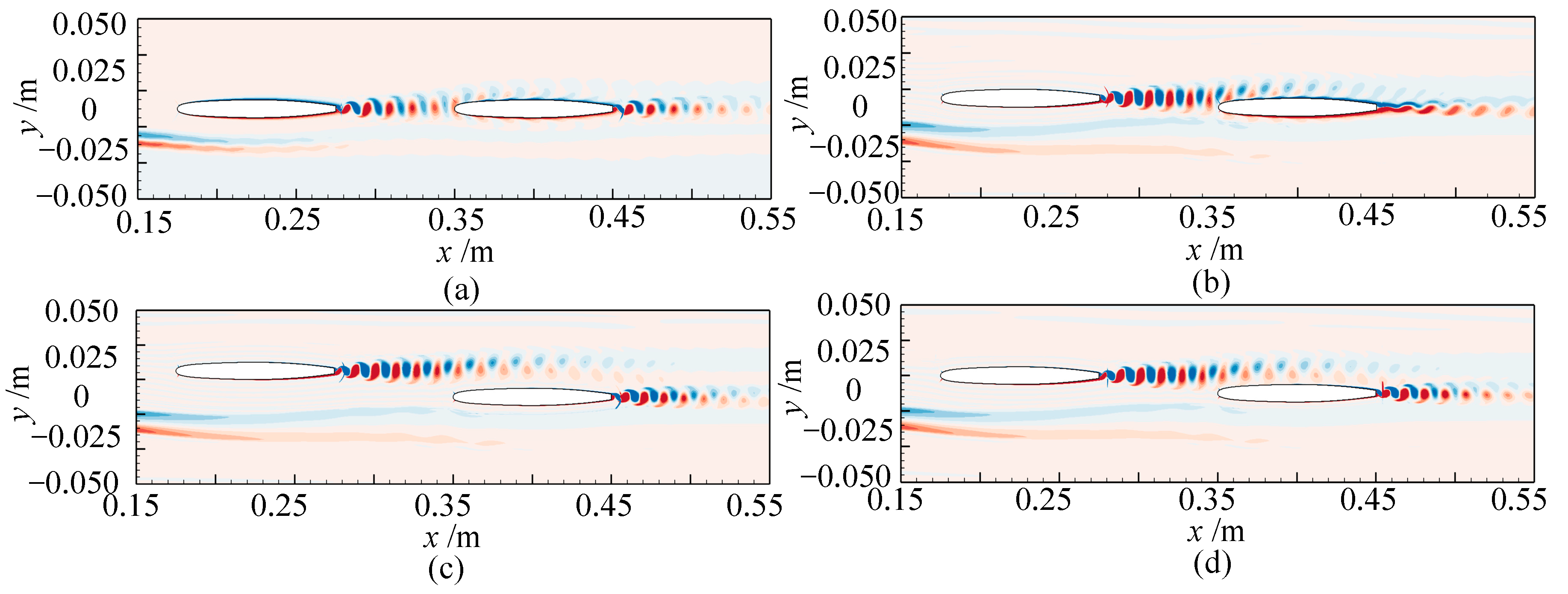
Figure 18 shows the vorticity distribution at different clocking positions. It can be clearly observed that under the four positions, the wake of the first stage hydrofoil has a greater impact on the secondary hydrofoil. At clocking position 4, the wake of the first hydrofoil almost dissipates when it reaches the secondary hydrofoil passage and cannot be observed. At the clocking positions 1, 2, and 3, the first hydrofoil wake is mixed with the mainstream region and boundary layer of the secondary hydrofoils. Since the mainstream belongs to high-energy fluid, and the wake belongs to low-energy fluid, its mixing loss is obviously greater than that of the boundary layer of the same low-energy fluid, resulting in a vibration difference.
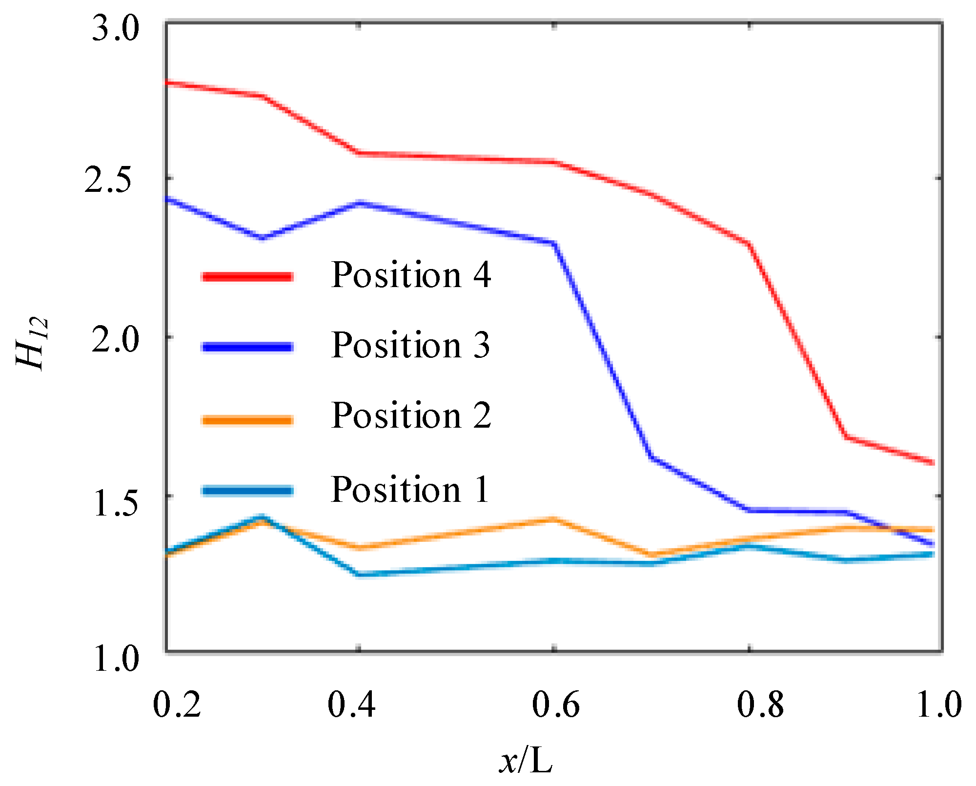
Figure 19 shows the change of the shape factor of the suction surface of the secondary hydrofoil. It can be seen that under the condition of clocking position 1, no matter how the valve opening changes, the shape factor of the whole hydrofoil surface is less than 1.5, which reflects that the whole hydrofoil area is turbulent. On the suction surface, the momentum of the fluid in the boundary layer of the first hydrofoil wake and the secondary-stage hydrofoil is exchanged, and the momentum of the boundary layer increases compared with that without the influence of the wake. With the introduction of high energy, the boundary layer becomes thinner, and the separation area decreases, thus reducing the flow loss of the boundary layer. The high turbulence wake generated by the upstream hydrofoil will induce the transition of the downstream hydrofoil boundary layer. For clocking positions 3 and 4, the position where the transition occurs is also different, which indicates that with the change of clocking position, the wake begins to affect the boundary layer on the suction surface of the blade at a certain position downstream of the leading edge of the blade, and the wake induces the boundary layer to start transition before boundary layer separation.
6. Conclusions
In this article, the stall of centrifugal pump with guide vanes is studied by numerical simulation, and the following conclusions were obtained:
- (1)
- The double-hump characteristic was found in the head discharge curve by using the SAS model. Comparing the flow field characteristics at different flow rate conditions, it was found that the hump area close to the optimal working condition is caused by hydraulic loss, and the hump area far away from the optimal working condition point is caused by the combined action of Euler head and hydraulic loss. The SAS model can accurately calculate the wall friction loss, thus predicting the double hump phenomenon.
- (2)
- The pressure fluctuation and head characteristics at different clocking positions under stall conditions were obtained. It was found that when the guide vanes outlet in line with the volute tongue, the flow pattern of the volute and guide vane is good, so the head is high due to small hydraulic loss, and the pressure fluctuation is low.
- (3)
- The mechanism of clocking effect in the centrifugal pump with guide vanes was obtained by simplifying the hydrofoil. Based on the simplified hydrofoil, it can be found that the disturbance of wake to the boundary layer will affect the boundary layer transition and then affect the friction stress of the blade, resulting in the change of flow field pressure amplitude. When the downstream hydrofoil head area is always interfered with by the upstream hydrofoil wake, the wake of the low-energy fluid is mixed with the boundary layer of the same low-energy fluid. At this time, the boundary layer is in a turbulent state to avoid laminar flow separation, causing small vibration of the downstream hydrofoil, so the position where the guide vane’s outlet is in line with the volute tongue is most recommended.
Author Contributions
Software, D.A.; Validation, W.H.; Writing—original draft, C.Y.; Supervision, Y.H. and Y.Z. All authors have read and agreed to the published version of the manuscript.
Funding
This research was funded by the National Natural Science Foundation of China (grant number: 52209109, No.52271275) and the Open Research Subject of Key Laboratory of Fluid and Power Machinery (Xihua University), Ministry of Education (grant number: LTDL-2022005).
Data Availability Statement
Not applicable.
Acknowledgments
The authors would like to acknowledge the financial support given by the National Natural Science Foundation of China (No.52209109, No.52271275) and the Open Research Subject of Key Laboratory of Fluid and Power Machinery (Xihua University), Ministry of Education (grant number LTDL-2022005).
Conflicts of Interest
The authors declare no conflict of interest.
Nomenclature
| Qd | Design flow | SAS | Scale adaptive simulation |
| Cu | Circumferential component of absolute velocity | LES | Large eddy simulation method |
| U | Circumferential velocity | RANS | Reynolds average method |
| HEnter | Euler head | Cp | Pressure coefficient |
| ΔCu·U | Euler energy | ω | Angular velocity |
References
- Wang, C.; Wang, F.; Li, C.; Chen, W.; Wang, H.; Lu, L. Investigation on energy conversion instability of pump mode in hydro-pneumatic energy storage system. J. Energy Storage 2022, 53, 105079. [Google Scholar] [CrossRef]
- Zhou, P.; Wang, F.; Mou, J. Investigation of rotating stall characteristics in a centrifugal pump impeller at low flow rates. Eng. Comput. 2017, 34, 1989–2000. [Google Scholar] [CrossRef]
- Feng, J.; Ge, Z.; Yang, H.; Zhu, G.; Li, C.; Luo, X. Rotating stall characteristics in the vaned diffuser of a centrifugal pump. Ocean Eng. 2021, 229, 108955. [Google Scholar] [CrossRef]
- Ye, C.L.; Wang, C.Y.; Zi, D.; Tang, Y.; van Esch, B.; Wang, F.J. Improvement of the SST γ-Reθt transition model for flows along a curved hydrofoil. J. Hydrodyn. 2021, 33, 520–533. [Google Scholar] [CrossRef]
- Stenning, A.H.; Kriebel, A.R. Stall propagation in a cascade of airfoils. Trans. Am. Soc. Mech. Eng. 1958, 80, 777–789. [Google Scholar] [CrossRef]
- Emmons, H.W.; Pearson, C.E.; Grant, H.P. Compressor surge and stall propagation. Trans. Am. Soc. Mech. Eng. 1955, 77, 455–467. [Google Scholar] [CrossRef]
- Day, I.J. Stall, surge and 75 years of research. ASME J. Turbomach. 2016, 138, 011001. [Google Scholar] [CrossRef]
- Zhang, N.; Gao, B.; Ni, D.; Liu, X. Coherence analysis to detect unsteady rotating stall phenomenon based on pressure pulsation signals of a centrifugal pump. Mech. Syst. Signal Process. 2021, 148, 107161. [Google Scholar] [CrossRef]
- Huang, X.-B.; Liu, Z.-Q.; Li, Y.-J.; Yang, W.; Guo, Q. Study of the internal characteristics of the stall in a centrifugal pump with a cubic non-linear SGS model. J. Hydrodyn. 2019, 31, 788–799. [Google Scholar] [CrossRef]
- Wang, C.; Wang, F.; Xie, L.; Wang, B.; Yao, Z.; Xiao, R. On the Vortical Characteristics of Horn-Like Vortices in Stator Corner Separation Flow in an Axial Flow Pump. J. Fluids Eng. 2021, 143, 061201. [Google Scholar] [CrossRef]
- Abusorrah, A.M.; Mebarek-Oudina, F.; Ahmadian, A.; Baleanu, D. Modeling of a MED-TVC desalination system by considering the effects of nanoparticles: Energetic and exergetic analysis. J. Therm. Anal. Calorim. 2021, 144, 2675–2687. [Google Scholar] [CrossRef]
- Hassan, M.; Mebarek-Oudina, F.; Faisal, A.; Ghafar, A.; Ismail, A. Thermal energy and mass transport of shear thinning fluid under effects of low to high shear rate viscosity. Int. J. Thermofluids 2022, 15, 100176. [Google Scholar] [CrossRef]
- Wang, C.; Wang, F.; Li, C.; Ye, C.; Yan, T.; Zou, Z. A modified STRUCT model for efficient engineering computations of turbulent flows in hydro-energy machinery. Int. J. Heat Fluid Flow 2020, 85, 108628. [Google Scholar] [CrossRef]
- Posa, A. LES investigation on the dependence of the flow through a centrifugal pump on the diffuser geometry. Int. J. Heat Fluid Flow 2021, 87, 108750. [Google Scholar] [CrossRef]
- Sano, T.; Yoshida, Y.; Tsujimoto, Y.; Nakamura, Y.; Matsushima, T. Numerical Study of Rotating Stall in a Pump Vaned Diffuser. J. Fluids Eng. 2002, 124, 363–370. [Google Scholar] [CrossRef]
- Braun, O. Part Load Flow in Radial Centrifugal Pumps. Ph.D. Thesis, EPFL, Lausanne, Switzerland, 2009. [Google Scholar]
- Lucius, A.; Brenner, G. Unsteady CFD simulations of a pump in part load conditions using scale-adaptive simulation. Int. J. Heat Fluid Flow 2010, 31, 1113–1118. [Google Scholar] [CrossRef]
- Zhang, N.; Jiang, J.; Gao, B.; Liu, X. DDES analysis of unsteady flow evolution and pressure pulsation at off-design condition of a centrifugal pump. Renew. Energy 2020, 153, 193–204. [Google Scholar] [CrossRef]
- Ji, L.; Li, W.; Shi, W.; Tian, F.; Agarwal, R. Effect of blade thickness on rotating stall of mixed-flow pump using entropy generation analysis. Energy 2021, 236, 121381. [Google Scholar] [CrossRef]
- Kan, K.; Zheng, Y.; Chen, Y.; Xie, Z.; Yang, G.; Yang, C. Numerical study on the internal flow characteristics of an axial-flow pump under stall conditions. J. Mech. Sci. Technol. 2018, 32, 4683–4695. [Google Scholar] [CrossRef]
- Krause, N.; Pap, E.R.; The´ venin, D. Influence of the blade geometry on flow instabilities in a radial pump elucidated by time-resolved particle-image velocimetry. In Proceedings of the Turbo Expo: Power for Land, Sea, and Air, Montreal, Canada, 14–17 May 2007; ASME: New York, NY, USA, 2007; Volume 47950, pp. 1659–1668. [Google Scholar]
- Berten, S.; Dupont, P.; Fabre, L.; Kayal, M.; Avellan, F.; Farhat, M. Experimental investigation of flow instabilities and rotating stall in a high-energy centrifugal pump stage. In Proceedings of the Fluids Engineering Division Summer Meeting, Vali, CO, USA, 2–6 August 2009; Volume 43727, pp. 505–513. [Google Scholar]
- Chudina, M. Noise as an indicator of cavitation in a centrifugal pump. Acoust. Phys. 2003, 49, 463–474. [Google Scholar] [CrossRef]
- Johnson, D.A.; Pedersen, N.; Jacobsen, C.B. Measurements of rotating stall inside a centrifugal pump impeller. In Proceedings of the Fluids Engineering Division Summer Meeting, Houston, TX, USA, 19–23 June 2005; Volume 41987, pp. 1281–1288. [Google Scholar]
- Ye, W.; Huang, R.; Jiang, Z.; Li, X.; Zhu, Z.; Luo, X. Instability analysis under part-load conditions in centrifugal pump. J. Mech. Sci. Technol. 2019, 33, 269–278. [Google Scholar] [CrossRef] [Green Version]
- Ren, X.; Fan, H.; Xie, Z.; Liu, B. Stationary stall phenomenon and pressure fluctuation in a centrifugal pump at partial load condition. Heat Mass Transf. 2019, 55, 2277–2288. [Google Scholar] [CrossRef]
- Takamine, T.; Furukawa, D.; Watanabe, S.; Watanabe, H.; Miyagawa, K. Experimental Analysis of Diffuser Rotating Stallin a Three-Stage Centrifugal Pump. Int. J. Fluid Mach. Syst. 2018, 11, 77–84. [Google Scholar] [CrossRef]
- Liu, X.-D.; Li, Y.-J.; Liu, Z.-Q.; Yang, W.; Tao, R. Dynamic evolution process of rotating stall vortex based on high-frequency PIV system in centrifugal impeller. Ocean Eng. 2022, 259, 111944. [Google Scholar] [CrossRef]
- Pavesi, G.; Cavazzini, G.; Ardizzon, G. Time–frequency characterization of the unsteady phenomena in a centrifugal pump. Int. J. Heat Fluid Flow 2008, 29, 1527–1540. [Google Scholar] [CrossRef]
- Takao, S.; Konno, S.; Ejiri, S.; Miyabe, M. Suppression of Diffuser Rotating Stall in A Centrifugal Pump by Use of Slit Vane. In Proceedings of the Fluids Engineering Division Summer Meeting, Online, 10–12 August 2021; American Society of Mechanical Engineers: New York, NY, USA, 2021; Volume 85291, p. V002T03A007. [Google Scholar]
- Yan, H.; Heng, Y.; Zheng, Y.; Tao, R.; Ye, C. Investigation on Pressure Fluctuation of the Impellers of a Double-Entry Two-Stage Double Suction Centrifugal Pump. Water 2022, 14, 4065. [Google Scholar] [CrossRef]
- Griffini, D.; Insinna, M.; Salvadori, S.; Martelli, F. Clocking Effects of Inlet Nonuniformities in a Fully Cooled High-Pressure Vane: A Conjugate Heat Transfer Analysis. J. Turbomach. 2015, 138, 021006. [Google Scholar] [CrossRef]
- Benigni, H.; Jaberg, H.; Yeung, H.; Salisbury, T.; Berry, O.; Collins, T. Numerical Simulation of Low Specific Speed American Petroleum Institute Pumps in Part-Load Operation and Comparison with Test Rig Results. J. Fluids Eng. 2012, 134, 024501. [Google Scholar] [CrossRef]
- Gu, Y.; Pei, J.; Yuan, S.; Wang, W.; Zhang, F.; Wang, P.; Liu, Y. Clocking effect of vaned diffuser on hydraulic performance of high-power pump by using the numerical flow loss visualization method. Energy 2019, 170, 986–997. [Google Scholar] [CrossRef]
- Wang, W.; Pei, J.; Yuan, S.; Yin, T. Experimental investigation on clocking effect of vaned diffuser on performance characteristics and pressure pulsations in a centrifugal pump. Exp. Therm. Fluid Sci. 2018, 90, 286–298. [Google Scholar] [CrossRef]
- Tan, M.; Lian, Y.; Wu, X.; Liu, H. Numerical investigation of clocking effect of impellers on a multistage pump. Eng. Comput. 2019, 36, 1469–1482. [Google Scholar] [CrossRef]
- Menter, F.R. Improved Two-Equation k-Turbulence Models for Aerodynamic Flows; NASA Technical Memorandum, 103975(1_), 3t; NASA: Washington, DC, USA, 1992.
- Hellsten, A. Some improvements in Menter’s k-omega SST turbulence model. In Proceedings of the 29th AIAA, Fluid Dynamics Conference, Albuquerque, NM, USA, 15–18 June 1998; p. 2554. [Google Scholar]
- Menter, F.R.; Egorov, Y. SAS turbulence modelling of technical flows. In Direct and Large-Eddy Simulation VI; Springer: Dordrecht, The Netherlands, 2006; pp. 687–694. [Google Scholar]
- Pedersen, N. Experimental Investigation of Flow Structures in a Centrifugal Pump Impeller Using Particle Image Velocimetry. Ph.D. Thesis, Technical University of Denmark, Kongens Lyngby, Denmark, 2000. [Google Scholar]
- Li, D.; Song, Y.; Lin, S.; Wang, H.; Qin, Y.; Wei, X. Effect mechanism of cavitation on the hump characteristic of a pump-turbine. Renew. Energy 2020, 167, 369–383. [Google Scholar] [CrossRef]
- Yan, H.; Zhang, H.; Zhou, L.; Liu, Z.; Zeng, Y. Optimization design of the unsmooth bionic structure of a hydrofoil leading edge based on the Grey–Taguchi method. Proc. Inst. Mech. Eng. Part M J. sEng. Marit. Environ. 2022, 14750902221128140. [Google Scholar] [CrossRef]
Figure 1.
Schematic Diagram of Guide-vane Centrifugal Pump.

Figure 2.
Grid of the centrifugal pump: (a) impeller; (b) guide vane; (c) volute.

Figure 3.
Centrifugal Pump Head Performance Curve.

Figure 4.
Comparison Diagram of Euler Head of Guide Vane Centrifugal Pump.

Figure 5.
Calculation of Total Head Loss of Guide-Vane Centrifugal Pump in Full Flow Channel.

Figure 6.
Calculation of Head Loss of Each Component of Guide-Vane Centrifugal Pump. (a) Inlet pipe; (b) Impeller; (c) Guide vane; (d) Volute.
Figure 6.
Calculation of Head Loss of Each Component of Guide-Vane Centrifugal Pump. (a) Inlet pipe; (b) Impeller; (c) Guide vane; (d) Volute.

Figure 7.
Pressure Contour and Streamline of Centrifugal Pump Calculated by SAS model. (a) 0.3 Qd; (b) 0.5 Qd; (c) 0.7 Qd.
Figure 7.
Pressure Contour and Streamline of Centrifugal Pump Calculated by SAS model. (a) 0.3 Qd; (b) 0.5 Qd; (c) 0.7 Qd.

Figure 8.
Pressure Contour and Streamline of Centrifugal Pump Calculated by SST k-ω model. (a) 0.3 Qd; (b) 0.5 Qd; (c) 0.7 Qd.
Figure 8.
Pressure Contour and Streamline of Centrifugal Pump Calculated by SST k-ω model. (a) 0.3 Qd; (b) 0.5 Qd; (c) 0.7 Qd.

Figure 9.
Clocking Position of the Pump. (a) Clocking position 1; (b) Clocking position 2; (c) Clocking position 3; (d) Clocking position 4.
Figure 9.
Clocking Position of the Pump. (a) Clocking position 1; (b) Clocking position 2; (c) Clocking position 3; (d) Clocking position 4.


Figure 10.
Centrifugal Pump Head Flow Curve at Different Clocking Positions.

Figure 11.
Velocity Streamline at Different Clocking Positions. (a) Clocking position 1; (b) Clocking position 2; (c) Clocking position 3; (d) Clocking position 4.
Figure 11.
Velocity Streamline at Different Clocking Positions. (a) Clocking position 1; (b) Clocking position 2; (c) Clocking position 3; (d) Clocking position 4.

Figure 12.
Pressure Fluctuation of Impeller and Guide Vane. (a) Monitor point R2; (b) Monitor point S2.
Figure 12.
Pressure Fluctuation of Impeller and Guide Vane. (a) Monitor point R2; (b) Monitor point S2.

Figure 13.
Pressure Fluctuation of Volute. (a) Monitor point W1 near tongue; (b) Monitor point W8 near outlet.
Figure 13.
Pressure Fluctuation of Volute. (a) Monitor point W1 near tongue; (b) Monitor point W8 near outlet.

Figure 14.
Simplified Hydrofoil. (a) Position 1; (b) Position 2; (c) Position 3; (d) Position 4.

Figure 15.
Variation of Lift, Drag Coefficient of Secondary Hydrofoil. (a) Lift; (b) Drag.

Figure 16.
Arrangement of Pressure Fluctuation Measuring Points.

Figure 17.
Pressure Distribution of Different Monitoring Points with Valve Opening. (a) Monitoring point P1; (b) Monitoring point P2; (c) Monitoring point P3; (d) Monitoring point P4.
Figure 17.
Pressure Distribution of Different Monitoring Points with Valve Opening. (a) Monitoring point P1; (b) Monitoring point P2; (c) Monitoring point P3; (d) Monitoring point P4.

Figure 18.
Vorticity Distribution at Different Time Sequence Positions. (a) Position 1; (b) Position 2; (c) Position 3; (d) Position 4.
Figure 18.
Vorticity Distribution at Different Time Sequence Positions. (a) Position 1; (b) Position 2; (c) Position 3; (d) Position 4.

Figure 19.
Change of Shape Factor of Suction Surface of Secondary Hydrofoil.

Disclaimer/Publisher’s Note: The statements, opinions and data contained in all publications are solely those of the individual author(s) and contributor(s) and not of MDPI and/or the editor(s). MDPI and/or the editor(s) disclaim responsibility for any injury to people or property resulting from any ideas, methods, instructions or products referred to in the content. |
© 2022 by the authors. Licensee MDPI, Basel, Switzerland. This article is an open access article distributed under the terms and conditions of the Creative Commons Attribution (CC BY) license (https://creativecommons.org/licenses/by/4.0/).
Share and Cite
MDPI and ACS Style
Ye, C.; An, D.; Huang, W.; Heng, Y.; Zheng, Y. Investigation on Stall Characteristics of Centrifugal Pump with Guide Vanes. Water 2023, 15, 21. https://doi.org/10.3390/w15010021
AMA Style
Ye C, An D, Huang W, Heng Y, Zheng Y. Investigation on Stall Characteristics of Centrifugal Pump with Guide Vanes. Water. 2023; 15(1):21. https://doi.org/10.3390/w15010021
Chicago/Turabian StyleYe, Changliang, Dongsen An, Wanru Huang, Yaguang Heng, and Yuan Zheng. 2023. "Investigation on Stall Characteristics of Centrifugal Pump with Guide Vanes" Water 15, no. 1: 21. https://doi.org/10.3390/w15010021
Note that from the first issue of 2016, this journal uses article numbers instead of page numbers. See further details here.