

Research on Surface Water Quality Assessment and Its Driving Factors: A Case Study in Taizhou City, China


1
School of Resources & Environment Sciences, Nanjing Agricultural University, Nanjing 210095, China
2
Taizhou Bureau of Agriculture and Rural Affairs, Taizhou 225300, China
3
Environmental Monitoring Center of Taizhou Ecological Environment Bureau, Taizhou 225300, China
*
Author to whom correspondence should be addressed.
Water 2023, 15(1), 26; https://doi.org/10.3390/w15010026
Submission received: 7 November 2022
/
Revised: 14 December 2022
/
Accepted: 17 December 2022
/
Published: 21 December 2022
(This article belongs to the Topic Hydrosphere under the Driving of Human Activity and Climate Change: Status, Evolution and Strategies)
Abstract
:It is necessary to assess and analyze the factors that influence surface water since they are crucial to human activities such as agriculture, raising livestock, and industry. Previous research has mostly focused on how land use and landscape patterns affect the quality of surface waters; it has seldom addressed the industrial and agricultural production activities that are directly connected to human society. Therefore, the research area’s surface water quality was assessed by single factor index (SFI) and composite water quality index (WQI), divided into flood and non-flood periods, and water quality indicators with severe pollution and significant seasonal variations were selected; A total of 28 indicators were selected from three main factors-topography, socio-economic, and land use type-and analyzed using the Spearman correlation coefficient model. (1) SFI data reveal substantial seasonal changes in pH, DO, NH3-N, TN, and TP water quality indicators. The well-developed agricultural and aquaculture in the studied region is the primary cause of the excess TN and NH3-N concentrations; (2) The sample points’ water quality index (WQI) scores range from 50 to 80, with 62% of them having “medium” water quality; (3) The study area’s seasonal variation in water quality is primarily caused by human socio-economic activities (GDP, industrial effluent discharge, COD discharge, aquatic product quality, and the proportion of primary, secondary, and tertiary industries), as well as land use type (forest, shrubland, and cropland). Topography has little effect on the study area’s surface water quality. This study offers a fresh viewpoint on surface water quality management and driver analysis, and a new framework for managing and safeguarding aquatic ecosystems.
1. Introduction
The enormous risk of depletion and pollution facing the world’s water resources may be attributed mostly to the misuse of water resources and pollution caused by the rise in human demand [1,2]. The degradation of water quality and the scarcity of water are two signs of the worldwide water deficit [3,4,5]. The two most significant water sources in the natural world are surface water and groundwater [6]. Both fluoride [7] and nitrate [8] are common pollutants in groundwater, with high nitrate levels and fluoride pollution affecting the vast majority of groundwater [9]. Surface water pollution has a greater potential than groundwater contamination, and the environmental implications of climate change have been a major threat to surface water quality [10], with human activities seen as the most significant cause of the worsening of surface water quality in many nations and areas throughout the world in recent decades [11]. The conflict between people and water resources has gotten worse as a result of the rapid expansion of society and the economy as well as the acceleration of global climate change. As a result, the creation of water management plans, including the creation of precise and logical techniques to evaluate surface water quality, is necessary [12]. Assessing the current state of water quality in the river basin and its driving factors is critical for understanding how geography, human socio-economics, and land use impact water quality changes [13,14]. A new problem is presently being faced in how to precisely identify the important variables that influence water quality due to the numerous water quality monitoring indicators and the intricate pollution process [15].
A surface water quality assessment [16] compares collected data to predetermined criteria for physical, chemical, nutritional, and biological indicators of the river to provide a qualitative or quantitative evaluation of the river’s water quality. The Chinese government’s method for assessing water quality in reports on water quality monitoring is known as single-factor assessment (SFA) [17]. To establish the water quality grade, the surface water environmental quality standards (e.g., GB3838-2002 (2002)) are used to choose the worst monitoring indications out of all monitoring indicators. The estimate of the water quality risk level is simplified by this technique, which is quick and straightforward yet yields conservative evaluation findings [18]. The development of the water quality index (WQI) approach [19] offers a solution to this issue. The Water Quality Index (WQI) is a mathematical tool that can combine a lot of water quality data into a single value [20], accurately analyze the water quality and eutrophication level of the water body, and offer the general public and decision-makers with a description of the current water quality situation and an evaluation of the water quality trends indicator [21]. The combination of the two approaches enables a new level of assessment of the water quality state of the research area and its geographical and temporal features, even though the two methods have distinct evaluation criteria and provide different findings. In this study, data on river water quality were combined with standards for the environmental quality of China’s surface waters using SFA and WQI methods. Subtle differences in water quality were identified, and indicators with notable seasonal differences in water were chosen to investigate the factors that influence changes in water quality.
Numerous academics have investigated the causes of surface water quality change in recent years, including analyzing the effects of climate change and land use on water quality [22]. Precipitation, temperature, and evapotranspiration are a few of the variables that affect water quality due to the climate [5,23,24]. However, human-driven land use change has emerged as a significant driver of both terrestrial and aquatic ecosystems [25]. Rivers play a significant role in determining the types of land uses, natural vegetation is commonly related to the quality of the water [26], and urban and agricultural land contributes to the global rise in nutrients and sediments in freshwater ecosystems [27]. According to Shi’s [28] research, the percentage of different land use types in a river basin has a significant impact on the water quality of rivers, as does the pattern of the landscape, size, density, aggregation, and variety of land use types. In Brazil, low-order river basins and riparian zones have been investigated at length by Mello et al. [29]. They discovered that forests have a significant role in preserving the water quality of low-order rivers, whereas agriculture and urban development are the primary causes of water quality deterioration. In the Qingyi River Basin in China, Yang et al. [30] investigated the effects of land use and landscape patterns on water quality. The findings demonstrated that cropland and construction land had negative effects on water quality and positive correlations with NH4+-N, TP, and EC. The ability of forest land to filter water pollution was shown to be positively connected with DO.
These studies, however, coupled land-use type changes with human activities and lacked the data necessary to define the variables that affect water quality [22]. Changes in land use are only one aspect of human activity; other contributing elements, such as industrial and agricultural operations, sewage discharge and treatment, etc., also have a role. In other words, the combined influence of climatic and land use changes on water quality should be less than but not equal to 100% [31]. As a result, changes in land use cannot accurately reflect the whole spectrum of human activities. The natural topography and human socio-economic activity have an influence on water quality in addition to climate and land use, which cannot be disregarded. As a result, the terrain [32] (elevation, slope, and aspect) and socioeconomic [33] variables are used in this study (population density, sewage discharge, livestock and poultry production, aquatic production, proportion of primary, secondary and tertiary industries, and the number of fertilizers and pesticides applied). various forms of land use (urban land, wetlands, aquatic bodies, cropland, forest land, shrubland, and grassland) to investigate the effects on watershed water quality.
The hydrological influence of land use, climate change, and human activities has been studied in several nations, and the study methodologies may be broadly classified into three groups [34]: the paired catchment approach, hydrological modeling, and statistical analysis. In small experimental catchments, the paired catchment approach [35,36] is often regarded as a popular technique for mitigating the effects of climate change. Its greatest applicable range is a small watershed area of 100 Km2, but it is challenging to apply to watersheds outside of this small region. A conceptual foundation for understanding the link between climate and water resources is provided by hydrological modeling [30]. The Soil and Water Assessment Tool (SWAT) model is a commonly used tool for hydrological research all over the world. It is based on physical, basin-scale hydrophysical processes and requires a significant amount of data and parameter inputs, which are frequently unavailable in some regions due to time or financial constraints, especially in some developing countries [37]. The SWAT model also lays greater emphasis on the hydrology of the entire watershed’s continuous time-scale process of topography, soil [38], and weather than it does on how human activities impact water quality [39]. An efficient way to assess the effects of human activity on water quality is using statistical analysis [34], which is straightforward and simple to use. Given that river water quality monitoring will provide a sizable and ongoing time series of data, several statistical approaches are utilized for analysis and discrimination, and sample sites may be categorized to demonstrate the link between water quality [40]. Analyzes hydrological, climatic, topographic, and human activity data from monitoring stations situated inside and around the research region to provide valid judgments about the link between hydrological responses and variables influencing water quality. Correlation analysis can be well used to investigate the relationship between water quality variables, and for continuous observation time series data, it is more necessary to use statistical methods to deal with the nature of correlation in random variable series [41].
Taizhou City is located in the central region of Jiangsu Province in China, with copious water resources but a dense population and significant water pollution. Urbanization, agriculturalization, and industrialization have increased freshwater consumption and pollution, altered the geographical and temporal distribution of water quality, and resulted in more complicated repercussions on water resources and hydrological processes, social development, and the economy in Taizhou and even the Yangtze River estuary. Therefore, this study used data from 12 state-controlled monitoring sections in Taizhou from 2020 to 2021, separated into flood season and non-flood season, to evaluate the present situation of river water quality in Taizhou by computing the water quality single factor index (SFI) and water quality index (WQI). The river water quality indicators with substantial seasonal variations were chosen, and the Spearman correlation coefficient model was used to examine the relationship between river water quality and topography, social economy, and land use, with the goal of (1) evaluating Taizhou City’s water quality; (2) Identify the major pollutant parameters and influencing variables of natural and human activities in Taizhou City throughout the flood and non-flood seasons, and offer scientific support for the healthy development of water ecology in Taizhou City, Jiangsu Province.
2. Materials and Methods
2.1. Study Area
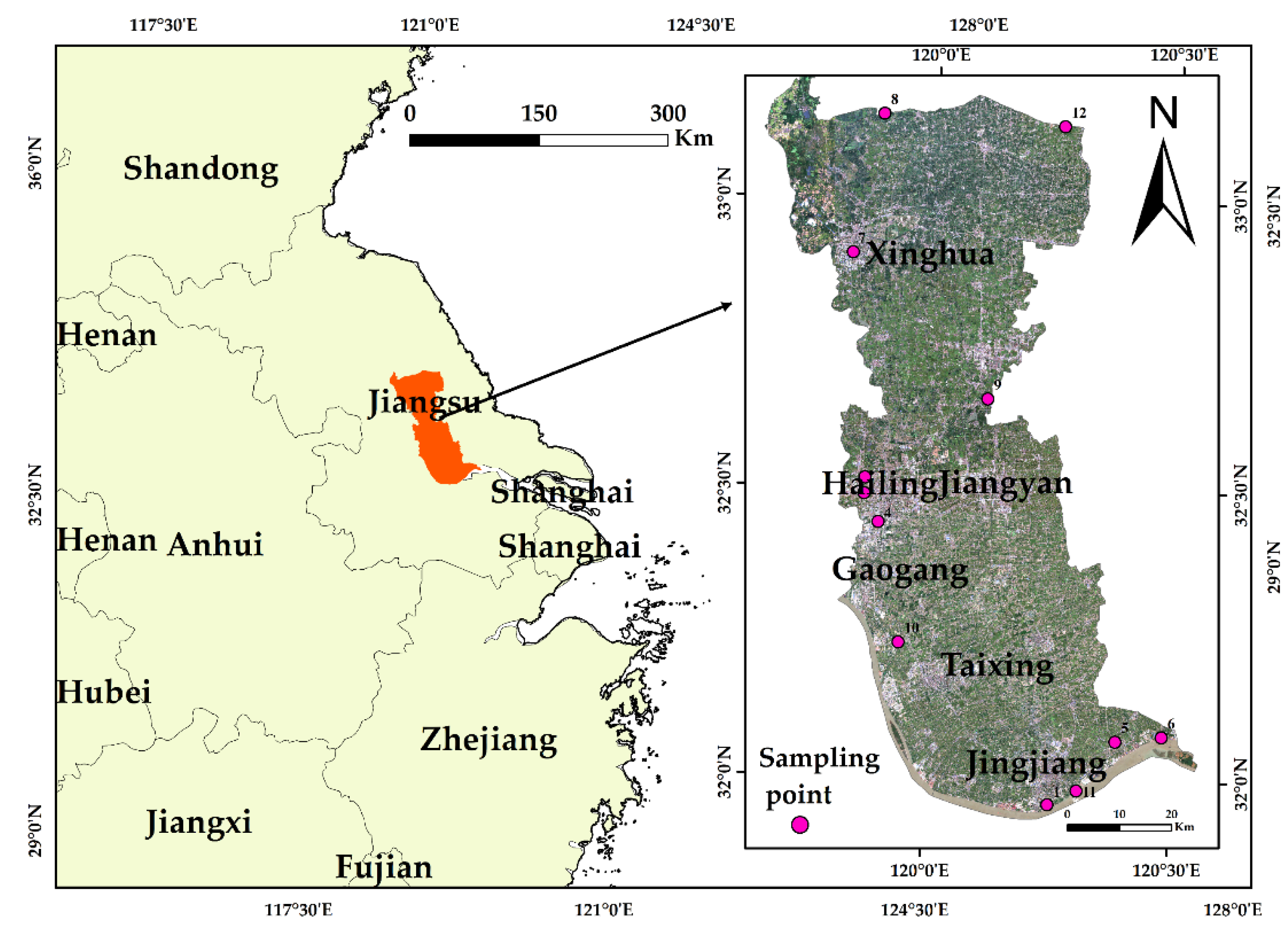
The research area of this study is Taizhou (119°38′24″ E~120°32′20″ E, 32°01′57″ N~33°10′59″ N, as shown in Figure 1), which has 3 districts under the jurisdiction of Hailing District, Gaogang District, and Jiangyan District, etc., and manages 3 cities at the county level, Xinghua City, Jingjiang City, and Taixing City, with an area of 5787 Km2, of which 77.85% is land area and 22.15% is water area. The territory’s river network is extensive and intertwined, and the rivers are generally bordered by the Tong Yang Highway, with the Huai River basin to the north of the road and the Yangtze River basin to the south.
The study location has a flat terrain. Except for an isolated hill in Jingjiang, the remainder is the alluvial plains of the two major river systems, the Jianghuai and Huaihe Rivers. With an elevation of 2–5 m along the river in the south, 5–7 m in the Gaosha region in the middle, and 1.5–5 m in the north Lixiahe area, the terrain is high in the middle and low in the north and south. In the north subtropical humid zone, Taizhou has a subtropical humid monsoon climate with overt monsoon features, including hot and rainy summers and warm, sparsely precipitated winters.
The research area’s permanent population was 4.5218 million as of 2021, and its GDP was 602.526 billion yuan. Among these, the primary industry’s added value increased by 2.8% to 31.813 billion yuan, while the secondary industry’s added value increased by 9.3% to 291.859 billion yuan. The tertiary industry-added value increased by 11.8% to 278.854 trillion yuan. Additionally, The research area has built an industrial system centered on the health sector, with assistance from the manufacturing sector, in the core region of the Yangtze River Delta. The textile industry, the chemical and pharmaceutical industries, the new material industries, and the high-tech shipbuilding industries are among the top industries. Meanwhile, It has established an “8 + N” agricultural industrial chain structure, with the major body consisting of grain and oil, livestock and poultry, river crabs, fruits and vegetables, freshwater fish and shrimp, leisure agriculture, flower gardening, and food seasoning. The agricultural areas of Lixiahe in the north, Gaosha in the middle, and the Yangtze River agricultural area in the south have all been constructed. To create a green development of agriculture, green recycling agriculture, emission reduction, and low carbon are simultaneous goals.
2.2. Data Source and Processing
The main data and its sources are as follows.
- (1)
- The water quality information is sourced from the China Surface Water Quality Automatic Monitoring Real-time Data Release System from 2021 to 2022. (https://szzdjc.cnemc.cn:8070/GJZ/Business/Publish/Main.html accessed on 23 May 2022). The China Environmental Monitoring Center is the provider of the system. The information is derived from the newly constructed and fully operational China Surface Water Quality Automatic Monitoring Station. Check the water quality every 4 h and publish the most recent information. Monitoring indexes included water temperature (WT), pH, Dissolved oxygen (DO), Electrical conductivity (EC), Permanganate index (CODMn), Chemical oxygen demand (COD), Five days biochemical oxygen demand (BOD5), Ammonia nitrogen (NH3-N), Total nitrogen (TN), and Total phosphorus (TP).
- (2)
- Topographic data such as elevation, slope and aspect affect rainfall and surface runoff by influencing the hydrothermal distribution and vegetation growth in the catchment, which further affects the generation and transport of non-point source pollution [32], therefore, this paper selects elevation, slope and aspect factors to explore the influence of topography on water quality distribution patterns. Elevation data is 30 m × 30 m spatial resolution DEM data, downloaded form geospatial data cloud (http://www.gscloud.con/ accessed on 15 March 2022);
- (3)
- The immediate reasons for the decline in water quality on the surface include excessive industrial and agricultural effluent discharge and unsustainable industrial structures [42]. Therefore, this paper selects population density, total sewage discharge, chemical oxygen demand (COD) emissions, pork production, poultry production, aquatic product production, the proportion of primary, secondary and tertiary industries, fertilizer and pesticide use, and other factors to explore the socio-economic impact on the distribution pattern of surface water quality. Socio-economic data from Taizhou Statistical Yearbook and National Economic and Social Development Bulletin;
- (4)
- According to studies, the percentage of different land use types in the watershed has a substantial impact on the water quality of rivers, as do landscape patterns, size, density, aggregation, and variety of land use types [28]. As a result, the statistical unit for the percentage of land cover types was chosen as the 12 km buffer zone [33] with a high correlation to the concentration of water quality parameters, and eight land use types—cropland, forest, grassland, shrub land, wetland, water body, bare land, and urban land—were chosen to investigate their effects on the distribution pattern of water quality. The European Space Agency (ESA) released the 2020 Global Land Cover product (https://biewer.esa-worldcover.org/worldcover accessed on 27 April 2022), which is where the data on land use is taken from. The spatial resolution is 10 m × 10 m, and the total classification accuracy is 74.4%.
The selection index of each element is shown in Table 1.
This research looked at water quality during the flood season (FS) and the non-flood season (NFS). According to the quantity of precipitation, May through September in the study area was categorized as the flood season, while all other months were labeled as the non-flood season. The water quality monitoring locations in the research area were distributed in 12 provincially regulated sectors (Figure 1 and Table 2). Water samples were collected in compliance with the “Environmental Quality Standards for Surface Water” established by China (GB3838-2002). DO use portable water quality testing analyzer YSI (yellow springs instrument. Zhejiang Luheng Environmental Technology, Hangzhou, China) for on-site measurement of the water body at 25 cm below the water surface, pH and water temperature using online water quality detector for determination, NH3-N, TN, TP determination methods for “water quality Determination of ammonia nitrogen salicylic acid spectrophotometric method” (HJ536-2009), “water quality Determination of total nitrogen The methods for the determination of COD, CODMn and BOD5 are “Determination of Chemical Oxygen Demand (COD) by Dichromate Method” (HJ828-2017), “Determination of Water Quality (COD) by Dichromate Method” (HJ828-2017) and “Determination of Water Quality (COD) by Ammonium Molybdate” (HJ670-2013). Determination of permanganate index” (GB/T 11892-1989), “Determination of five-day biochemical oxygen demand of water quality Dilution and inoculation method” (HJ505-2009).
2.3. Water Quality Assessment Methods
2.3.1. Single Factor Pollution Index
Single factor pollution index (SFI) is assessed based on the relationship between water quality metrics and benchmark values [27,28], and various pollution parameter types are computed in different methods [17].
If the value of the index is smaller, the better, as permanganate index and ammonia concentration, then:
If the value of the index is bigger, the better, as dissolved oxygen, then:
If the value of the index is closer to a certain value, the better pH value, then:
where the pollution index is Pi and Ci is the measured value of water quality parameter i, the maximum value of the evaluation standard is Si (here we used the boundary value of class II in surface water quality standard ((GB3838-2002), Table 3), Cmax is the saturated concentration of the evaluation factor, Smax and Smin are the highest and lowest average value of the evaluation standard respectively, and Siave is the average value of the highest and lowest evaluation criteria of the pollutant.
The saturation concentration of DO is:
where T is the temperature, and the unit is °C.
2.3.2. Water Quality Index
The water quality measures (DO, EC, CODMn, BOD5, NH3-N, TN, and TP) were chosen as assessment indicators, and the water quality index (WQI) was utilized to assess Taizhou’s water quality in 2021–2022. The WQI scale ranges from 0 to 100, and Table 4 [43] lists its evaluation criteria.
Four stages are taken to determine the WQI [44]:
- (1)
- Selection of key parameters;
- (2)
- Converting important parameters to a common scale was accomplished by applying sub-index curves to convert each parameter to a scale from 0 to 100 [45]. The sub-index curves might be segmented-lined, segmented-nonlinear, linear, nonlinear, etc;
- (3)
- Assigning weights to parameters;
- (4)
- Aggregation of indices to produce a WQI.
The generic equation of WQI [46] is:
where WQI is the comprehensive water quality index, Hi is the standardized value of the ith water quality parameter, Pi is the weight of the ith water quality parameter, and n is the number of water quality parameters involved in the evaluation. Pi values range from 1 to 4, where 4 represents the most important parameter for the survival of aquatic organisms (such as dissolved oxygen) and 1 represents the parameter that affects aquatic life (such as chlorine), as shown in Table 5.
2.4. Spearman’s Correlation Coefficient
A statistical technique called correlation analysis analyzes the interdependence of data patterns to determine the relationships between variables [47]. Calculating the Spearman correlation coefficient to measure the size of the correlation between two sets of data is a common correlation analysis approach. To evaluate the monotonic connection between two variables, the Spearman correlation coefficient, a nonparametric statistical correlation measure, is utilized [48]. Since the observed indicators of water quality do not follow a normal distribution, the Spearman coefficient is employed to analyze the pattern of correlation between the different factors. The degree and direction of any monotonic link between two rank variables or a rank variable and a measured variable are quantified by the Spearman correlation coefficient rs, a distribution-free rank statistical measure [49]. A negative (−) correlation happens if one variable declines while the other grows, and vice versa. A positive (+) correlation occurs when two variables increase or decrease equally. The expression for rs is [50]:
where is the difference between each pair of ranking variables, N is the total number of samples, and the value of rs is between −1 and 1.
3. Results
3.1. Assessment of Water Quality in Taizhou
3.1.1. Assessment of SFI
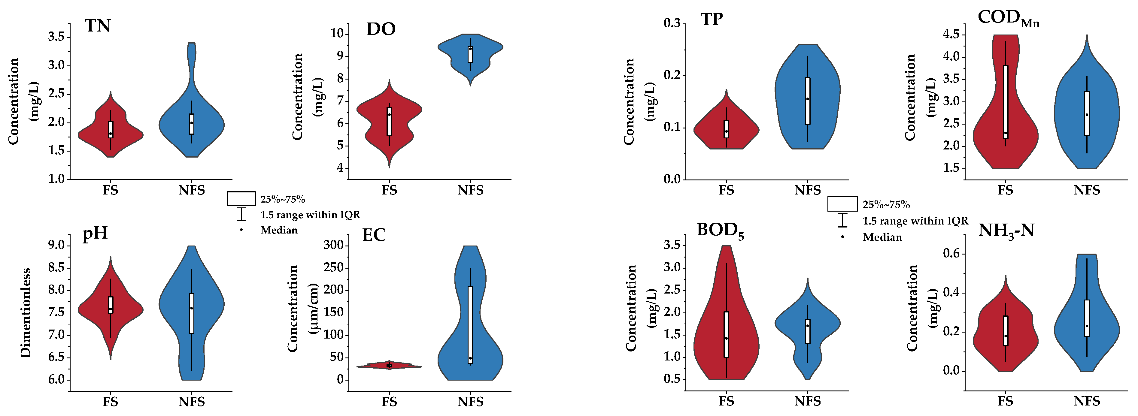
There are noticeable discrepancies in the water quality parameters in the flood season (FS) and the non-flood season (NFS) in Taizhou from January 2021 to May 2022, according to distribution data (Figure 2) and descriptive statistics (Table 6). There are significant seasonal variations in DO, EC, BOD5, NH3-N, and TN. BOD5 average concentration during the flood season (4.28 mg/L) is 2.63 times higher than the average concentration during the non-flood season (1.63 mg/L); NH3-N and TN average concentration during the flood season (1.22 mg/L, 1.18 mg/L) was twice as high as average concentration during the non-flood season (0.63 mg/L, 0.65 mg/L); however, average DO concentration during the flood season (6.14 mg/L) was only about 2/3 in non-flood season. Changes in NH3-N and TN exhibit obvious seasonal variations as well. and the two water quality metrics’ average concentrations were much greater during the flood season than they were during the non-flood season. The non-flood season had a wider range of EC variation than the flood season did, as seen by the bigger standard deviation (5.69 vs. 156.60) and coefficient of variation (0.17 vs. 1.41) in the non-flood season.
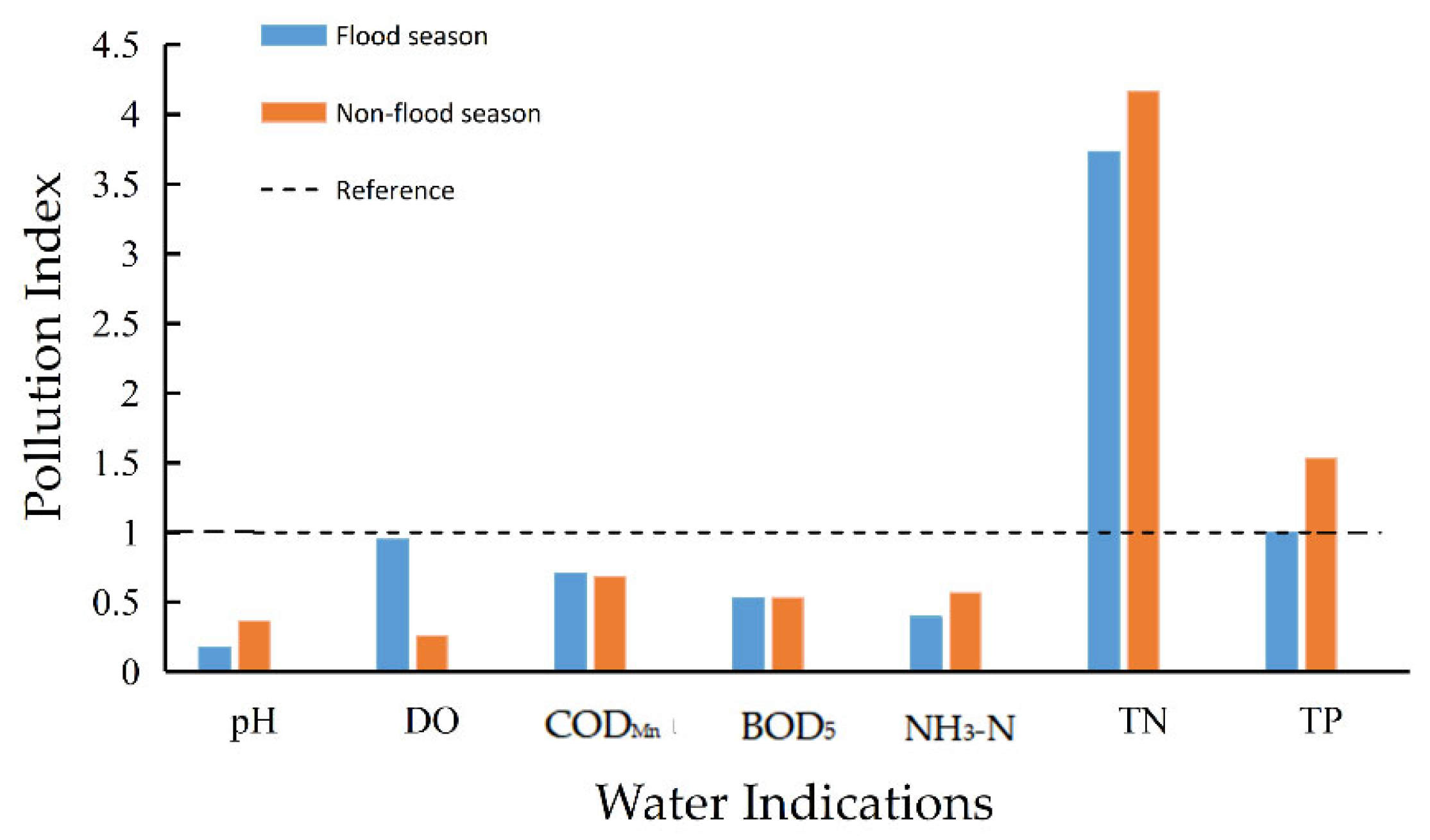
Except for CODMn and BOD5, the findings of the single-factor evaluation demonstrate (Figure 3) that the five indicators of pH, DO, NH3-N, TN, and TP in the research region exhibit obvious hydrological seasonal changes. The biggest seasonal variance was seen in DO, followed by TP, and TN. Among these, the distribution trends of the pH, NH3-N, TN, and TP pollution indices values indicated that the flood season was smaller than the non-flood season, although the DO index indicated the contrary. The pollution index was higher during the flood season than during the non-flood season. The primary pollution indicator during the flood season is TN, and the accompanying pollution index is 3.73; in contrast, during the non-flood season, the main pollution indications are TN and TP, and the corresponding pollution indices are 4.16 and 1.53, respectively. As a result, TN and TP indicators with severe pollution in flood and non-flood seasons, as well as DO with large seasonal changes, were chosen to conduct a thorough water quality evaluation and analysis of influencing variables on a macro scale.
3.1.2. Assessment of WQI
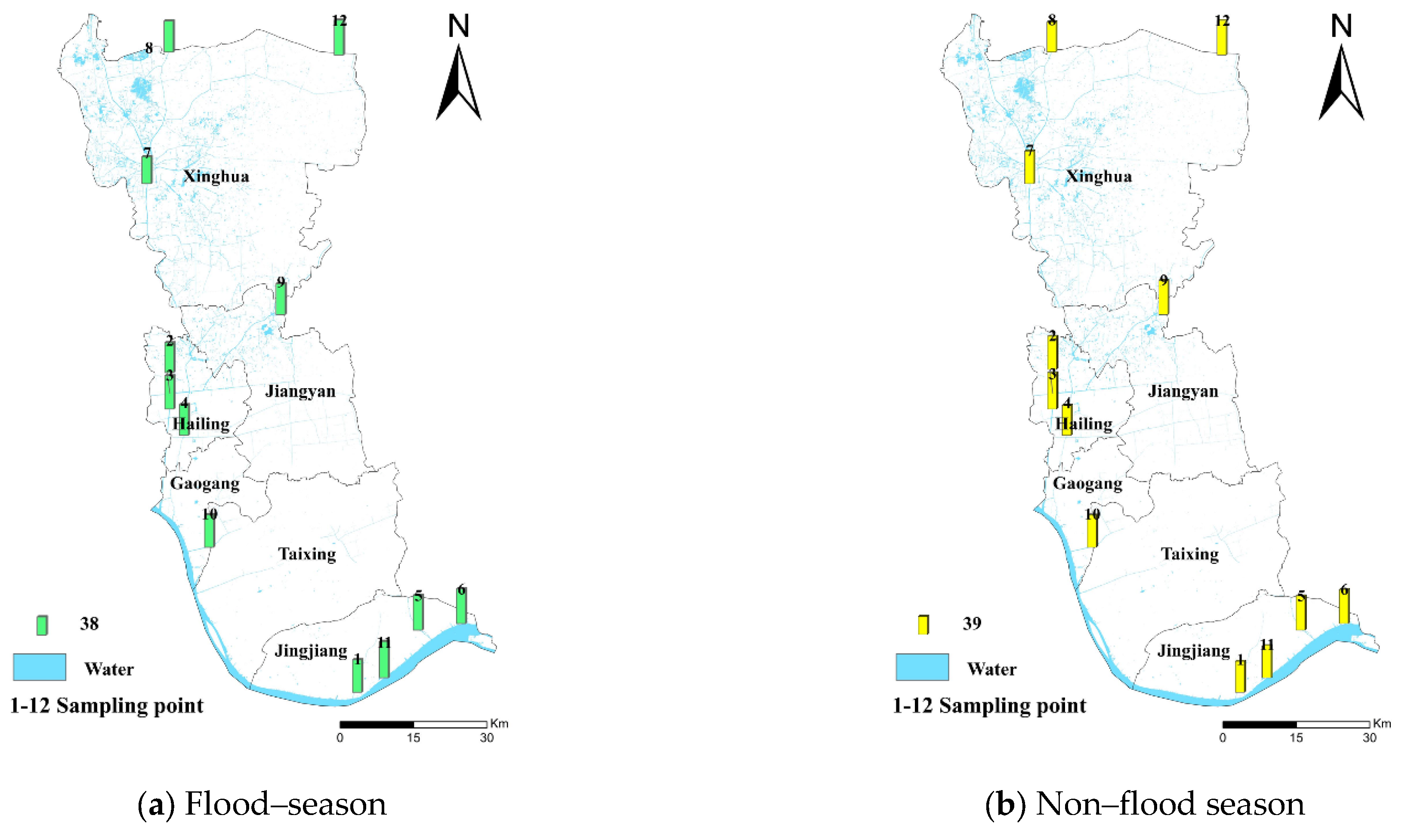
In the research region, Figure 4 depicts the dispersion of the WQI index throughout the flood season and non-flood season. As can be observed, there are no appreciable differences in WQI values in the study region between the flood season and the non-flood season. The most substantial shift in WQI occurs in the southwest of the research region, specifically the west of Hailing District, Gaogang District, Taixing, and Jingjiang. This area’s WQI value during flood season is between 70 and 90, whereas its WQI value during the non-flood season is between 50 and 70. Water quality is better during flood season than during the non-flood season. During the flood season, the Study area’s average WQI score is 67, which is typically considered to be in the “medium” level. The WQI value of 67% of the sample stations is below 70, and the south has higher water quality than the north. The average WQI value during the non-flood season is 71, which is at the “good” threshold. In the non-flood season, the central region’s water quality is somewhat better than that of the other areas, and the WQI value is below 70 at close to 58% of the sample locations. Overall, the study area’s water quality score (WQI) falls into the 50–80 range, which is considered to be of “medium” quality.
3.2. Spearman Correlation Analysis
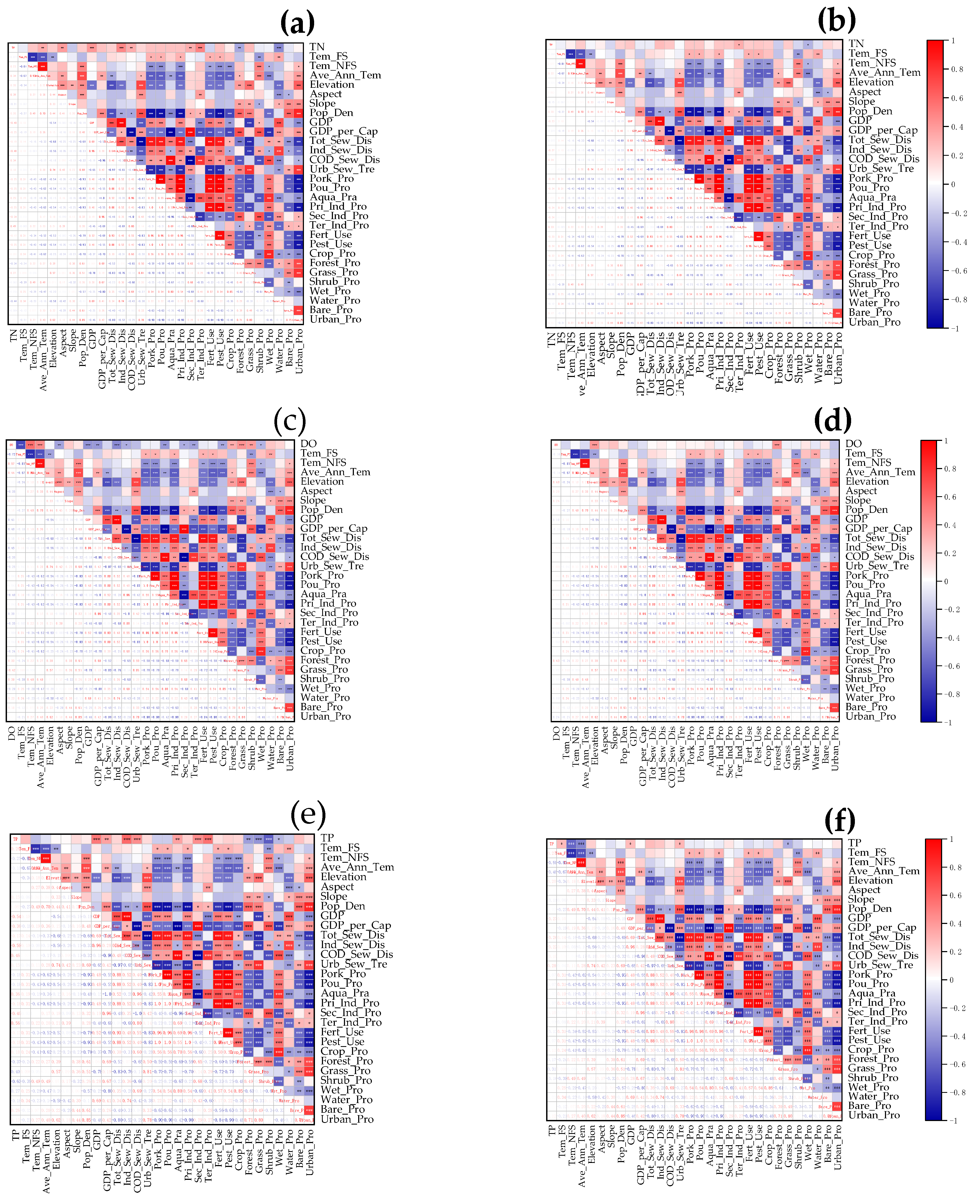
To perform Spearman correlation analysis [42], choose the concentrations of three generally used water quality measures such as TN, TP, and DO, which have notable water quality concerns in both flood season and non-flood season, as well as the WQI comprehensive water quality assessment index and three types of driving variables such as topographical, human socio-economic activity, and land use type. The results are given in Figure 5. To facilitate comparison, the results are summarized in Table 7.
The result shows that during the flood season, the concentration of TN was substantially linked negatively with five indicators, including the proportion of forest land area (r = −0.34, p < 0.01) and the proportion of water area (r = −0.44, p < 0.01), and considerably positively with seven indicators, including COD discharge (r = 0.34, p < 0.01), GDP (r = 0.40, p < 0.001), and total sewage discharge (r = 0.48, p < 0.001). According to Figure 5b, the primary factor controlling TN concentration during non-flood seasons is the fraction of wetland and forest area, which is inversely connected with wetland area (r = −0.28, p < 0.05) and forest area (r = −0.19, p < 0.05); had a substantial (r = 0.33, p < 0.05) positive correlation with the percentage of the tertiary industry.
During the flood season, the concentration of TP was significantly negatively correlated with four indicators including the proportion of forest area (r = −0.37, p < 0.01), the proportion of shrub area (r = −0.63, p < 0.001), and the proportion of wetland area (r = −0.27, p < 0.05), at the same time, with COD emissions (r = 0.46, p < 0.001), aquatic product production (r = 0.36, p < 0.01) and GDP ((r = 0.54, p < 0.01) < 0.001) and other seven indicators showed a significant positive correlation. The TP concentration in the non-flood season was significantly negatively correlated with the proportion of grassland area (r = −0.31, p < 0.01), the average annual water temperature (r = −0.48, p < 0.001), and was significantly positively correlated with GDP (r = 0.27, p < 0.05), and the urban sewage treatment rate (r = 0.28, p < 0.05).
DO concentrations during the flood season were negatively correlated with ten indicators including flood water temperature (r = −0.72, p < 0.001), COD emissions (r = −0.30, p < 0.01), GDP (r = −0.41, p < 0.001), the proportion of cropland area (r = −0.34, p < 0.01) and industrial sewage discharge (r = −0.45, p < 0.001). Six indicators were significantly positively correlated including non-flood water temperature (r = 0.57, p < 0.001), average annual water temperature (r = 0.44, p < 0.001), and the proportion of forest area (r = 0.33, p < 0.01). The non-flood season DO concentration driver was relatively simple and significantly positively correlated with two indicators: the proportion of forest area (r = 0.43, p < 0.001) and elevation (r = 0.40, p < 0.01). Other indicators were not significantly correlated with the non-flood DO concentration.
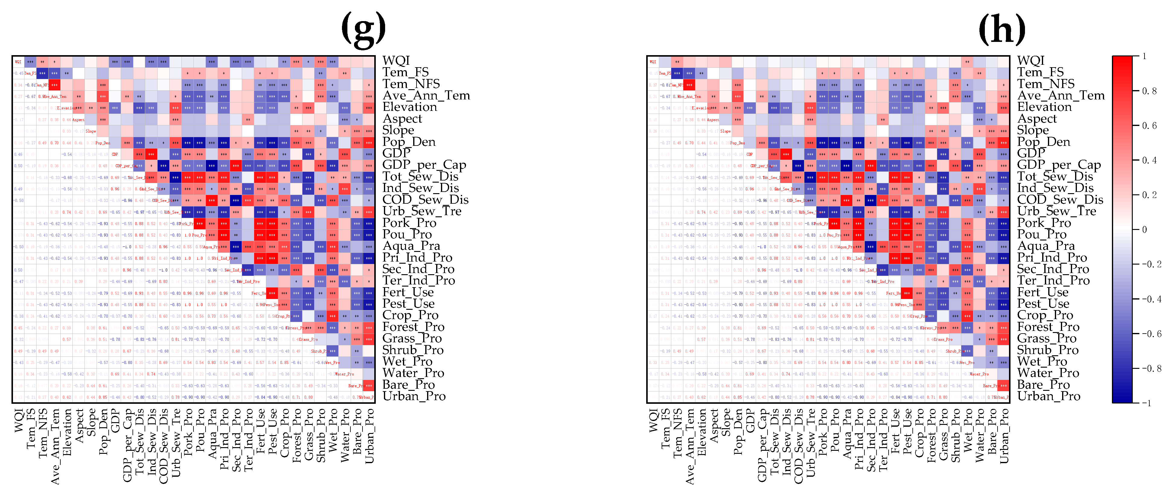
Flood season WQI index and proportion of cropland (r = −0.38, p < 0.01), flood season temperature (r = −0.45, p < 0.001), industrial sewage discharge (r = −0.49, p < 0.001) and GDP (r = −0.50, p < 0.001) and other ten indicators were significantly negatively correlated; at the same time, with the proportion of forest area (r = 0.45, p < 0.001), the proportion of shrub area (r = 0.50, p < 0.001) and the proportion of wetland area (r = 0.43, p < 0.001) were significantly positively correlated. The driving mechanism of WQI in non-flood season is relatively simple, and there is a significant positive correlation between WQI in non-flood season and the proportion of wetland area (r = 0.33, p < 0.01) and temperature in non-flood season (r = 0.37, p < 0.001), and other indicators were not significantly correlated with WQI concentration in non-flood seasons.
4. Discussion
4.1. Main Factors Influencing Water Quality
The driving force study revealed that land use, particularly the usage of forest, shrub, and agriculture, as well as human socioeconomic activities (GDP, industrial sewage, and COD discharge), are significant driving forces influencing changes in the water quality of Taizhou rivers. The combined influence of natural elements and human activities needs to be taken into account to elucidate the variables that affect water quality.
4.1.1. Impact of Anthropogenic Activities
The primary causes of excessive N and P in rivers are GDP, COD brought on by industrial growth, and non-point source pollution brought on by excessive sewage discharge; however, the presence of forest areas and wetlands can prevent the accumulation of N and P concentrations. A considerable share is accounted for by Taizhou’s coal mines, nonferrous metals, papermaking, fertilizer manufacture, and other important water pollutant discharge sectors. Unreasonable industrial construction and sewage discharge will seriously harm the aquatic environment. According to data, Taizhou utilized 73.03% of the total industrial energy in 2020, with heavy industry using the majority of it, followed by light industry. Furthermore, population increase has resulted in the discharge of a huge volume of sewage from residents’ homes, as well as the eutrophication of water bodies driven by chemical fertilizers and pesticides used in industrial and agricultural operations [51]. In the same year, 144,930 tons of chemical fertilizers (in pure form) were utilized in Taizhou City, a 1.4% reduction from the year before. Although there has been a yearly decline in Taizhou City’s use of chemical fertilizers since 2016, the rate of use is still rather low. Crops are unable to absorb 45–65% of N and P. Some of them reach the water body with the scouring of rains, which raises the chance that groundwater and runoff carrying nitrogen and phosphorus fertilizer nutrients may pollute the river and worsen its richness. According to research by Peng [52] and colleagues, the primary input sources of nitrate in surface water remote from metropolitan areas include nitrate fertilizer, soil ammonium, manure, and septic tank waste. The driving factors of water quality in the watershed were investigated [33], and it was discovered that nitrogen and phosphorus nutrients released from production and living in Guangzhou, as well as human landscape alterations, were the primary causes of non-point source pollution. Furthermore, unrecycled livestock and domestic sewage provide 63% of nitrogen and phosphorus emissions in freshwater [53]. Taizhou is situated in the plain area of the Yangtze River’s middle and lower sections. It serves as a significant hub for the production of grain, oil, and freshwater goods in China. Over 31.94% of the population works in agriculture. Rural regions have a thriving freshwater crab farming sector. Rivers, livestock, and poultry breeding [54], particularly the release of manure and urine brought on by pig breeding, cause rivers to contain an excessive amount of N and P, which raises the risk of river pollution.
Land use has been significantly impacted by human activities throughout the world, having an impact on watersheds and their ecosystems [55]. Land use in watersheds can also have an impact on rivers and the overall quality of the ecosystem [56], which in turn modifies the community composition by changing the hydrological, physicochemical, and benthic habitat conditions. Taizhou is located in the Yangtze River Basin and the Huai River Basin. The intricate river network system creates a pattern of land usage in which Taizhou is built by water and born by water. The influence of land use and human activities on river ecosystems and water quality is determined by a variety of factors, including riparian forest buffer zones, the size of the watershed buffer zone, the position of the reach within the watershed, the existence of additional pressures, and the land use measure [57]. The riparian zones allow sediment and pollutants to enter water bodies through surface runoff, groundwater flow, organic inputs, and atmospheric deposition [40], while the existence of built-up land hardens the underlying surface and weakens its retention and absorption of sediment and pollutants, leading to an increase in N and P concentrations in the watershed, and the increase in agricultural and urban land is also directly responsible for the increase in N and P concentrations in the watershed, which are both nutrient concentrations are in turn negatively correlated with increases in the percentage of the forest land area [58]. The percentage of agricultural land in Taizhou has risen from 68.34% to 70.10% during the last ten years. The expansion of agricultural land has resulted in a fall in the proportion of forest land and wetlands. Numerous studies have shown that the extent of agriculture and farmland in the catchment decreases water quality, habitat, and biological assemblages and that land use within the riparian zone and throughout the watershed is particularly successful in predicting TN, nitrate, and orthophosphate.
4.1.2. Impact of Natural Factors
According to Mackie [59] and other research, riparian zones can capture 89% of nitrogen and 80% of phosphorus. The potential of different types of natural vegetation to absorb nitrogen and phosphorus pollution varies significantly, whereas forest land and shrubs have a substantial capacity to do so [26]. The urban greenery coverage rate of 42.57% in Taizhou in 2020 is slightly higher than the average urban greenery coverage rate of 42.1% in China, and the higher urban greenery coverage allows shrubs and forest land to trap some of the pollutants lost to water bodies [60], and it is believed that riparian zone buffers covered by forestland have a positive impact on water quality, significantly reducing sediment loads and nitrogen and phosphorus nutrient concentrations in water, which can stabilize river channels and floodplains and control the flow of sediment, nutrients, and agricultural pollutants from plains and hillsides into rivers [61]. By limiting the geographical distribution and composition of various land uses, topography has an impact on the number of pollutants, the distribution of pollution sources, and even water quality [5]. The research location is in China’s Yangtze River Plain, where there is limited topographical undulation but a large number of river networks and significant potential for pollution movement and transformation. Distinct forms of land use play different roles in the paths from nonpoint sources to waterways [62]. Wang et al. [63] found that urban land use can also have adverse effects on rivers and water quality, especially when reaching critical quantities and close to river courses, the main changes associated with the increase in the urban land area include an increase in the number of pollutants in runoff transport, increased water temperature due to loss of riparian vegetation and exposure to surface runoff, and reduced channel and biological habitat structure due to limited sediment input and interactions between riparian and river margins [64]. Taizhou features densely populated cities and a high pace of urbanization. The city’s sewage discharge treatment rate was 96.39% in 2020, an 8.69% increase from 2015. The high sewage treatment rate may filter or remove most water contaminants, reducing pollutants released into rivers. The study concluded that there is not a strong association between urban land and river water quality since there are not a lot of urban lands close to the sample location. However, this does not imply that urban land does not affect Taizhou’s water quality. To further understand how Taizhou’s urban land affects the quality of its water, more sample locations should be established in the future. Furthermore, topography [42] and light [65] influence rainfall and runoff by influencing the distribution of water and heat in the watershed as well as vegetation growth, and the impact on river water quality cannot be overlooked.
4.2. Limitations
In this study, the influence of climate change on water quality was neglected and only the geography, socioeconomics, and land use variables were chosen to evaluate the association of watershed water quality. In actuality, changes in precipitation patterns, global warming, and human responses to climate change will all have a considerable impact on surface water quality [66,67]. Rain causes rivers to redistribute their water, which alters how nutrients are transported through the river. Wolf et al. [68] discovered that increases in annual nitrogen loading in the Iowa watershed, USA, were caused by increases in the river’s annual flow and annual base flow as a result of increasing precipitation in the watershed. In a study of seven rivers in the Midwest of the United States, Baeumler and Gupta [69] discovered that climate change, including changes in rainfall and temperature, was primarily to blame for the increase in nitrogen loads in these rivers. Changes in land use and fertilizer application had little impact on nitrogen load changes. Furthermore, the study area’s industrial business is developing, and the stainless steel and shipbuilding industries will discharge various chemical elements into the water body. Due to the insufficient study data, this work has not conducted extensive investigation to determine whether this has resulted in excessive heavy metals in the water body [70]. In the future, this is something that has to be taken into consideration.
The evaluation model in this work is constrained by the little amount of data and the short data period, which prevents accurate calibration and verification on an annual scale. Furthermore, changes in water quality are quite complicated, and monitoring the eight indicators alone is insufficient to predict water quality. To undertake a thorough and realistic evaluation of water quality in the future, the breadth and volume of data collecting should be expanded, and the influence of riparian ecosystems should be taken into account [71].
4.3. Water Quality Management
The United Nations has reclassified improving water quality as one of the top concerns on the global agenda [72]. Surface water quality in China has been seriously threatened during the past 40 years by the country’s rapid industrialization and urbanization [73]. As a result, a nationwide monitoring network with long-term access to water quality parameters is urgently required to allow dynamic real-time monitoring of water quality and collect reliable water quality data. To regulate the total water quality in China from a macro viewpoint, the government should also apply differentiated management of regional water quality indicators according to various areas and regulate water quality parameters, reference standards, regional variations, and water quality evaluation methodologies [74].
Most of the study area’s water pollution control infrastructure construction was finished in recent years, but there are still issues, including ineffective sewage treatment, rain and pollution flowing together, and a mismatch between sewage discharge standards and environmental protection requirements. The research area’s sewage discharge and treatment rate was 96.39% in 2020. The next level of water pollution control will put more of an emphasis on management requirements and criteria for water quality classification than it would on building infrastructure. The fecal discharge of tailwater is a critical remedy for the developing aquaculture and animal farming industries in the research region. As a result, the land used for raising livestock and poultry must be carefully planned. Changes to the land cover and crop planting zones should be made in extremely polluted regions, such as growing cash crops in the higher reaches of related rivers, reservoirs, and lakes rather than food crops. To enhance the quality of the water in the watershed, aquiculture zones should be divided into tailwater discharge categories, and Standardized manure disposal practices and standards for livestock and poultry production.
The analysis of the water quality metrics reveals that TN is the primary element influencing the management of water quality in the research region. Fertilizers, pesticides, and insecticides used in agricultural production are the primary sources of TN and NH3-N [75]. Water quality management focuses on lowering NH3-N in rivers owing to changes in assessment indicators, while disregarding the influence of nitrate on total water quality in the selection of criteria for WQI calculation. In reality, nitrate has turned into a common water contaminant as a result of nitrogen loss in agriculture and significant nitrate fertilizer use. Monitoring for nitrates shouldn’t be disregarded.
In the future, the remote online water quality monitoring system should be improved, the frequency and scope of monitoring water quality and related driving factors should be increased, and the main influencing variables of the water environment in different times and situations should be mined in combination with drones and satellite remote sensing big data, the level of water pollution tracing and emergency management should be improved, and the safety of drinking water should be improved.
5. Conclusions
This study assesses the water quality of Taizhou using SFA and WQI water quality assessment methodologies. It picks water quality indicators with substantial seasonal fluctuations and pollution levels and performs Spearman correlation analysis using topographical, socioeconomic, and land use data to investigate the driving factors of river water quality in Taizhou City. The results demonstrate that:
(1) The concentration of TN (1.18 mg/L) and NH3-N (1.22 mg/L) surpassing the norm are the primary causes of Taizhou’s water pollution, but the presence of TP (0.15 mg/L) over the threshold cannot be disregarded. There are noticeable changes between the hydrological seasons and driving variables of DO, BOD5, NH3-N, and TN. While DO concentrations are lower during flood seasons than during non-flood seasons, NH3-N, TN, and BOD5 concentrations are greater during flood seasons than during non-flood seasons, indicating that the factors affecting water quality during flood seasons are more complicated than during non-flood seasons. According to the WQI result, Taizhou’s water quality is generally good, with the center and northern regions of the city having the most surpassing points. When there is flood season, the water quality is higher than during the non-flood season.
(2) Seasonal variations in river water quality in Taizhou are significantly influenced by changes in land use, particularly changes in forest, shrub, and farmland, as well as increasing human industrial production activities (industrial sewage and COD discharge). The primary causes of the high concentration of TN and NH3-N and the deterioration of water quality are the vast amounts of nitrogen and phosphorus fertilizers released by human activities and the aggravation of man-made land landscapes.
Reducing the concentration of total nitrogen is a critical issue for water pollution control and management, creating a reasonable evaluation index system will be necessary for managing and controlling river water quality pollution in the future.
Author Contributions
Writing-original draft, S.D.; Writing-review and editing, S.D., C.L. and X.J.; Data curation, S.D.; Methodology, S.D. and C.L.; Software, S.D.; Investigation, S.D.; Visualization, C.L.; Formal acquisition, C.L.; Supervision, C.L., X.J., T.Z. and H.H.; Project administration, X.J., T.Z. and H.H.; Resources, C.L., X.J., T.Z. and H.H. All authors have read and agreed to the published version of the manuscript.
Funding
This work was supported by Development Research and Master Plan of Modern Agricultural Industry in the North Ecological Economic Zone of Taizhou City, China (Grant No.tzyjy100045).
Conflicts of Interest
The authors declare no conflict of interest.
References
- Alvarez, P.J.J.; Chan, C.K.; Elimelech, M.; Halas, N.J.; Villagran, D. Emerging opportunities for nanotechnology to enhance water security. Nat. Nanotechnol. 2018, 13, 634–641. [Google Scholar] [CrossRef] [PubMed]
- Bakker, K. Water Security Research: Challenges and Opportunities. Science 2012, 337, 914–915. [Google Scholar] [CrossRef]
- Nong, X.; Shao, D.; Zhong, H.; Liang, J. Evaluation of water quality in the South-to-North Water Diversion Project of China using the water quality index (WQI) method. Water Res. 2020, 178, 115781. [Google Scholar] [CrossRef]
- Yu, C.; Yin, X.; Li, H.; Yang, Z. A hybrid water-quality-index and grey water footprint assessment approach for comprehensively evaluating water resources utilization considering multiple pollutants. J. Clean. Prod. 2020, 248, 119225. [Google Scholar] [CrossRef]
- Wu, J.; Lu, J. Spatial scale effects of landscape metrics on stream water quality and their seasonal changes. Water Res. 2021, 191, 116811. [Google Scholar] [CrossRef] [PubMed]
- Carroll, S.; Liu, A.; Dawes, L.; Hargreaves, M.; Goonetilleke, A. Role of Land Use and Seasonal Factors in Water Quality Degradations. Water Resour. Manag. 2013, 27, 3433–3440. [Google Scholar] [CrossRef] [Green Version]
- Xiao, Y.; Liu, K.; Hao, Q.; Li, Y.; Xiao, D.; Zhang, Y. Occurrence, Controlling Factors and Health Hazards of Fluoride-Enriched Groundwater in the Lower Flood Plain of Yellow River, Northern China. Expo. Health 2022, 14, 345–358. [Google Scholar] [CrossRef]
- Xiao, Y.; Liu, K.; Hao, Q.; Xiao, D.; Zhu, Y.; Yin, S.; Zhang, Y. Hydrogeochemical insights into the signatures, genesis and sustainable perspective of nitrate enriched groundwater in the piedmont of Hutuo watershed, China. Catena 2022, 212, 106020. [Google Scholar] [CrossRef]
- Xiao, Y.; Hao, Q.; Zhang, Y.; Zhu, Y.; Yin, S.; Qin, L.; Li, X. Investigating sources, driving forces and potential health risks of nitrate and fluoride in groundwater of a typical alluvial fan plain. Sci. Total Environ. 2022, 802, 149909. [Google Scholar] [CrossRef]
- Uhl, A.; Hahn, H.J.; Jager, A.; Luftensteiner, T.; Siemensmeyer, T.; Doll, P.; Noack, M.; Schwenk, K.; Berkhoff, S.; Weiler, M.; et al. Making waves: Pulling the plug-Climate change effects will turn gaining into losing streams with detrimental effects on groundwater quality. Water Res. 2022, 220, 118649. [Google Scholar] [CrossRef]
- Zheng, L.; Jiang, C.; Chen, X.; Li, Y.; Li, C.; Zheng, L. Combining hydrochemistry and hydrogen and oxygen stable isotopes to reveal the influence of human activities on surface water quality in Chaohu Lake Basin. J. Environ. Manag. 2022, 312, 114933. [Google Scholar] [CrossRef] [PubMed]
- Mararakanye, N.; Le Roux, J.J.; Franke, A.C. Long-term water quality assessments under changing land use in a large semi-arid catchment in South Africa. Sci. Total Environ. 2022, 818, 151670. [Google Scholar] [CrossRef] [PubMed]
- Ahn, S.R.; Kim, S.J. Assessment of integrated watershed health based on the natural environment, hydrology, water quality, and aquatic ecology. Hydrol. Earth Syst. Sci. 2017, 21, 5583–5602. [Google Scholar] [CrossRef] [Green Version]
- Cook, N.A.; Sarver, E.A.; Krometis, L.H.; Huang, J. Habitat and water quality as drivers of ecological system health in Central Appalachia. Ecol. Eng. 2015, 84, 180–189. [Google Scholar] [CrossRef]
- Aboelnga, H.T.; El-Naser, H.; Ribbe, L.; Frechen, F.B. Assessing Water Security in Water-Scarce Cities: Applying the Integrated Urban Water Security Index (IUWSI) in Madaba, Jordan. Water 2020, 12, 1299. [Google Scholar] [CrossRef]
- Tango, P.J.; Batiuk, R.A. Chesapeake Bay recovery and factors affecting trends: Long-term monitoring, indicators, and insights. Reg. Stud. Mar. Sci. 2016, 4, 12–20. [Google Scholar] [CrossRef]
- Hu, Z.; Hu, L.; Cheng, H.; Qi, D. Application of Pollution Index Method Based on Dynamic Combination Weight to Water Quality Evaluation. Earth Environ. Sci. 2018, 153, 062008. [Google Scholar] [CrossRef] [Green Version]
- Xia, R.; Chen, Z. Integrated Water-Quality Assessment of the Huai River Basin in China. J. Hydrol. Eng. 2015, 20, 05014018. [Google Scholar] [CrossRef]
- Yan, F.; Liu, L.; Li, Y.; Zhang, Y.; Chen, M.; Xing, X. A dynamic water quality index model based on functional data analysis. Ecol. Indic. 2015, 57, 249–258. [Google Scholar] [CrossRef]
- Stambuk-Giljanovic, N. Water Quality Evaluation by Index in Dalmatia; ELsevier Science: Amsterdam, The Netherlands, 1999. [Google Scholar]
- Gazzaz, N.M.; Yusoff, M.K.; Aris, A.Z.; Juahir, H.; Ramli, M.F. Artificial neural network modeling of the water quality index for Kinta River (Malaysia) using water quality variables as predictors. Mar. Pollut. Bull. 2012, 64, 2409–2420. [Google Scholar] [CrossRef]
- Yunyun, L.; Jianjia, C.; Yimin, W.; Wenting, J.; Aijun, G. Spatiotemporal Impacts of Climate, Land Cover Change and Direct Human Activities on Runoff Variations in the Wei River Basin. Water 2016, 8, 220. [Google Scholar] [CrossRef] [Green Version]
- de Paul Obade, V.; Moore, R. Synthesizing water quality indicators from standardized geospatial information to remedy water security challenges: A review. Environ. Int. 2018, 119, 220–231. [Google Scholar] [CrossRef] [PubMed]
- Mian, H.R.; Saleem, S.; Hu, G.; Sadiq, R. Water Distribution Systems: Hydraulics and Quality Modeling. In Encyclopedia of Water; CRC press: Boca Raton, FL, USA, 2019; pp. 1–11. [Google Scholar]
- Zhang, J.; Guo, Q.; Du, C.; Wei, R. Quantifying the effect of anthropogenic activities on water quality change in the Yangtze River from 1981 to 2019. J. Clean. Prod. 2022, 363, 132415. [Google Scholar] [CrossRef]
- Taniwaki, R.H.; Cassiano, C.C.; Fransozi, A.A.; Vásquez, K.V.; Posada, R.G.; Velásquez, G.V.; Ferraz, S.F.B. Effects of land-use changes on structural characteristics of tropical high-altitude Andean headwater streams. Limnologica 2019, 74, 1–7. [Google Scholar] [CrossRef]
- de Mello, K.; Valente, R.A.; Ribeiro, M.P.; Randhir, T. Effects of forest cover pattern on water quality of low-order streams in an agricultural landscape in the Pirapora river basin, Brazil. Environ. Monit. Assess. 2022, 194, 189. [Google Scholar] [CrossRef] [PubMed]
- Shi, P.; Zhang, Y.; Li, Z.; Li, P.; Xu, G. Influence of land use and land cover patterns on seasonal water quality at multi-spatial scales. Catena 2017, 151, 182–190. [Google Scholar] [CrossRef]
- Mello, K.d.; Valente, R.A.; Randhir, T.O.; dos Santos, A.C.A.; Vettorazzi, C.A. Effects of land use and land cover on water quality of low-order streams in Southeastern Brazil: Watershed versus riparian zone. Catena 2018, 167, 130–138. [Google Scholar] [CrossRef]
- Qiangqiang, Y.; Guanglai, X.; Xiancheng, Y.; Aijuan, L.; Chen, C. Responses of water quality to land use and landscape pattern in the Qingyijiang River watershed. Acta Ecol. Sin. 2020, 40, 9048–9058. [Google Scholar] [CrossRef]
- Swain, S.; Taloor, A.K.; Dhal, L.; Sahoo, S.; Al-Ansari, N. Impact of climate change on groundwater hydrology: A comprehensive review and current status of the Indian hydrogeology. Appl. Water Sci. 2022, 12, 1–25. [Google Scholar] [CrossRef]
- Panuska, J.C.; Moore, I.D.; Kramer, L.A. Terrain analysis-integration into the agricultural non-point source (AGNPS) pollution model. J. Soil Water Conserv. 1991, 46, 59–64. [Google Scholar]
- Chen, J.; Chen, S.; Fu, R.; Yin, X.; Wang, C.; Li, D.; Peng, Y. Analysis of water quality status and driving factors in Guangdong Province. Acta Ecol. Sin. 2022, 42. [Google Scholar]
- Tan, M.L.; Ibrahim, A.L.; Yusop, Z.; Duan, Z.; Ling, L. Impacts of land-use and climate variability on hydrological components in the Johor River basin, Malaysia. Hydrol. Sci. J. 2015, 60, 873–889. [Google Scholar] [CrossRef]
- Lorup, J.K.; Refsgaard, J.C.; Mazvimavi, D. Assessing the effect of land use change on catchment runoff by combined use of statistical tests and hydrological modelling Case studies from Zimbabwe. J. Hydrol. 1998, 205, 147–163. [Google Scholar] [CrossRef]
- Li, Z.; Liu, W.-z.; Zhang, X.-c.; Zheng, F.-l. Impacts of land use change and climate variability on hydrology in an agricultural catchment on the Loess Plateau of China. J. Hydrol. 2009, 377, 35–42. [Google Scholar] [CrossRef]
- Wei, X.; Liu, W.; Zhou, P. Quantifying the Relative Contributions of Forest Change and Climatic Variability to Hydrology in Large Watersheds: A Critical Review of Research Methods. Water 2013, 5, 728–746. [Google Scholar] [CrossRef]
- Yuan, L.; Forshay, K.J. Evaluating Monthly Flow Prediction Based on SWAT and Support Vector Regression Coupled with Discrete Wavelet Transform. Water 2022, 14, 2649. [Google Scholar] [CrossRef]
- Karakuş, C.B. Evaluation of water quality of Kızılırmak River (Sivas/Turkey) using geo-statistical and multivariable statistical approaches. Environ. Dev. Sustain. 2019, 22, 4735–4769. [Google Scholar] [CrossRef]
- Zhang, Z.; Tao, F.; Du, J.; Shi, P.; Yu, D.; Meng, Y.; Sun, Y. Surface water quality and its control in a river with intensive human impacts--a case study of the Xiangjiang River, China. J. Environ. Manag. 2010, 91, 2483–2490. [Google Scholar] [CrossRef]
- Lehmann, A.; Rode, M. Long-term behaviour and cross-correlation water quality analysis of the river Elbe, Germany. Wat. Res. 2001, 35, 2153–2160. [Google Scholar] [CrossRef]
- Wang, X.; Liu, X.; Wang, L.; Yang, J.; Wan, X.; Liang, T. A holistic assessment of spatiotemporal variation, driving factors, and risks influencing river water quality in the northeastern Qinghai-Tibet Plateau. Sci. Total Environ. 2022, 851, 157942. [Google Scholar] [CrossRef]
- Jonnalagadda, S.B.; Mhere, G. Water quality of the Odzi River in the Eastern Highlands of Zimbabwe. Water Res. 2001, 35, 2371–2376. [Google Scholar] [CrossRef]
- Pak, H.Y.; Chuah, C.J.; Tan, M.L.; Yong, E.L.; Snyder, S.A. A framework for assessing the adequacy of Water Quality Index-Quantifying parameter sensitivity and uncertainties in missing values distribution. Sci. Total Environ. 2021, 751, 141982. [Google Scholar] [CrossRef]
- Pesce, F.S.; Wunderlin, A.D. Use of Water Quality Indices to Verify the Impact of Cordoba City (Argentina) on Suquýa River; ELsevier Science: Amsterdam, The Netherlands, 1999. [Google Scholar]
- Sánchez, E.; Colmenarejo, M.F.; Vicente, J.; Rubio, A.; García, M.G.; Travieso, L.; Borja, R. Use of the water quality index and dissolved oxygen deficit as simple indicators of watersheds pollution. Ecol. Indic. 2007, 7, 315–328. [Google Scholar] [CrossRef]
- Gejingting, X.; Ruiqiong, J.; Wei, W.; Libao, J.; Zhenjun, Y. Correlation analysis and causal analysis in the era of big data. Mater. Sci. Eng. 2019, 563, 042032. [Google Scholar] [CrossRef]
- Zhang, W.-Y.; Wei, Z.-W.; Wang, B.-H.; Han, X.-P. Measuring mixing patterns in complex networks by Spearman rank correlation coefficient. Phys. A Stat. Mech. Appl. 2016, 451, 440–450. [Google Scholar] [CrossRef]
- Xiao, C.; Ye, J.; Esteves, R.M.; Rong, C. Using Spearman’s correlation coefficients for exploratory data analysis on big dataset. Concurr. Comput. Pract. Exp. 2016, 28, 3866–3878. [Google Scholar] [CrossRef]
- Krishnaraj, A.; Deka, P.C. Spatial and temporal variations in river water quality of the Middle Ganga Basin using unsupervised machine learning techniques. Environ. Monit. Assess. 2020, 192, 744. [Google Scholar] [CrossRef]
- Tao, J.; Sun, X.H.; Cao, Y.; Ling, M.H. Evaluation of water quality and its driving forces in the Shaying River Basin with the grey relational analysis based on combination weighting. Environ. Sci. Pollut. Res. 2022, 29, 18103–18115. [Google Scholar] [CrossRef]
- Peng, J.; Zheng, B.; Wang, X.; Wang, M. The driving force of basin water resource utilization to lake nutrients. Hydrol. Sci. J. 2020, 65, 855–866. [Google Scholar] [CrossRef]
- Yan, K.; Xu, J.-C.; Gao, W.; Li, M.-J.; Yuan, Z.-W.; Zhang, F.-S.; Elser, J. Human perturbation on phosphorus cycles in one of China’s most eutrophicated lakes. Resour. Environ. Sustain. 2021, 4, 100026. [Google Scholar] [CrossRef]
- Zheng, L.; Zhang, Q.; Zhang, A.; Hussain, H.A.; Liu, X.; Yang, Z. Spatiotemporal characteristics of the bearing capacity of cropland based on manure nitrogen and phosphorus load in mainland China. J. Clean. Prod. 2019, 233, 601–610. [Google Scholar] [CrossRef]
- Measho, S.; Chen, B.; Pellikka, P.; Trisurat, Y.; Guo, L.; Sun, S.; Zhang, H. Land Use/Land Cover Changes and Associated Impacts on Water Yield Availability and Variations in the Mereb-Gash River Basin in the Horn of Africa. J. Geophys. Res. Biogeosciences 2020, 125, e2020JG005632. [Google Scholar] [CrossRef]
- Schuetz, T.; Gascuel-Odoux, C.; Durand, P.; Weiler, M. Nitrate sinks and sources as controls of spatio-temporal water quality dynamics in an agricultural headwater catchment. Hydrol. Earth Syst. Sci. 2016, 20, 843–857. [Google Scholar] [CrossRef] [Green Version]
- White, J.Y.; Walsh, C.J. Catchment-scale urbanization diminishes effects of habitat complexity on instream macroinvertebrate assemblages. Ecol. Appl. 2020, 30, e02199. [Google Scholar] [CrossRef]
- Kreiling, R.M.; Bartsch, L.A.; Perner, P.M.; Hlavacek, E.J.; Christensen, V.G. Riparian Forest Cover Modulates Phosphorus Storage and Nitrogen Cycling in Agricultural Stream Sediments. Environ. Manag. 2021, 68, 279–293. [Google Scholar] [CrossRef]
- Mackie, C.; Levison, J.; Binns, A.; O’Halloran, I. Groundwater-surface water interactions and agricultural nutrient transport in a Great Lakes clay plain system. J. Great Lakes Res. 2021, 47, 145–159. [Google Scholar] [CrossRef]
- Carter, L.D.; Dzialowski, A.R. Predicting sediment phosphorus release rates using landuse and water-quality data. Freshw. Sci. 2012, 31, 1214–1222. [Google Scholar] [CrossRef]
- Turunen, J.; Markkula, J.; Rajakallio, M.; Aroviita, J. Riparian forests mitigate harmful ecological effects of agricultural diffuse pollution in medium-sized streams. Sci. Total Environ. 2019, 649, 495–503. [Google Scholar] [CrossRef]
- Yu, S.; Xu, Z.; Wu, W.; Zuo, D. Effect of land use types on stream water quality under seasonal variation and topographic characteristics in the Wei River basin, China. Ecol. Indic. 2016, 60, 202–212. [Google Scholar] [CrossRef]
- WANG, L.; LYONS, J.; KANEHL, P. Impacts of urbanization on stream habitat and fish across multiple spatial scales. Environ. Manag. 2001, 28, 255–266. [Google Scholar] [CrossRef] [PubMed]
- Paul, M.J.; Meyer, J.L. Streams in the urban landscape. Annu. Rev. Ecol. Syst. 2001, 32, 333–365. [Google Scholar] [CrossRef]
- Hamid, A.; Bhat, S.U.; Jehangir, A. Local determinants influencing stream water quality. Appl. Water Sci. 2019, 10, 1–16. [Google Scholar] [CrossRef]
- Ryberg, K.R.; Chanat, J.G. Climate extremes as drivers of surface-water-quality trends in the United States. Sci. Total Environ. 2022, 809, 152165. [Google Scholar] [CrossRef]
- Murdoch, P.S.; Baron, J.S.; Miller, T.L. Potential effects of climate change on surface-water quality in North America. J. Am. Water Resour. Assoc. 2000, 36, 347–366. [Google Scholar] [CrossRef]
- Wolf, K.A.; Gupta, S.C.; Rosen, C.J. Precipitation Drives Nitrogen Load Variability in Three Iowa Rivers. J. Hydrol. Reg. Stud. 2020, 30, 100705. [Google Scholar] [CrossRef]
- Baeumler, N.W.; Gupta, S.C. Precipitation as the Primary Driver of Variability in River Nitrogen Loads in the Midwest United States. JAWRA J. Am. Water Resour. Assoc. 2019, 56, 113–133. [Google Scholar] [CrossRef]
- Rahman, M.A.T.M.T.; Paul, M.; Bhoumik, N.; Hassan, M.; Alam, M.K.; Aktar, Z. Heavy metal pollution assessment in the groundwater of the Meghna Ghat industrial area, Bangladesh, by using water pollution indices approach. Appl. Water Sci. 2020, 10, 1–15. [Google Scholar] [CrossRef]
- Hilary, B.; Chris, B.; North, B.E.; Angelica Maria, A.Z.; Sandra Lucia, A.Z.; Carlos Alberto, Q.G.; Beatriz, L.G.; Rachael, E.; Andrew, W. Riparian buffer length is more influential than width on river water quality: A case study in southern Costa Rica. J. Environ. Manag. 2021, 286, 112132. [Google Scholar] [CrossRef]
- Hanna, D.E.L.; Lehner, B.; Taranu, Z.E.; Solomon, C.T.; Bennett, E.M. The relationship between watershed protection and water quality: The case of Québec, Canada. Freshw. Sci. 2021, 40, 382–396. [Google Scholar] [CrossRef]
- Woo, S.Y.; Kim, S.J.; Lee, J.W.; Kim, S.H.; Kim, Y.W. Evaluating the impact of interbasin water transfer on water quality in the recipient river basin with SWAT. Sci. Total Environ. 2021, 776, 145984. [Google Scholar] [CrossRef]
- Guan, X.; Ren, X.; Tao, Y.; Chang, X.; Li, B. Study of the Water Environment Risk Assessment of the Upper Reaches of the Baiyangdian Lake, China. Water 2022, 14, 2557. [Google Scholar] [CrossRef]
- Li, J.L.; Zuo, Q.T. Forms of Nitrogen and Phosphorus in Suspended Solids: A Case Study of Lihu Lake, China. Sustainability 2020, 12, 5026. [Google Scholar] [CrossRef]
Figure 1.
Study area and location of sampling points.

Figure 2.
Distribution of water quality monitoring results.

Figure 3.
Distribution of single-factor pollution indices for water quality indicators in flood and non-flood periods.
Figure 3.
Distribution of single-factor pollution indices for water quality indicators in flood and non-flood periods.

Figure 4.
Spatial distribution of WQI evaluation results.

Figure 5.
Distribution of single factor pollution index. * p < 0.10, ** p < 0.05, *** p < 0.01. (a) TN actuation analysis in flood season; (b) TN actuation analysis in non-flood season; (c) TP actuation analysis in flood season; (d) TP actuation analysis in non-flood season; (e) DO actuation analysis in flood season; (f) DO actuation analysis in non-flood season; (g) WQI actuation analysis in flood season; (h) WQI actuation analysis in non-flood season.


Table 1.
Indicators of terrain, human society and economy and land use.
| Elements | Indicators | Contracted Form | Reference |
|---|---|---|---|
| Terrain factors | Elevation | Elevation | Panuska.J.C. et al. [32] |
| Aspect | Aspect | ||
| Slope | Slope | ||
| Social economic factors | The population density | Pop_Den | Chen Ijnyue. et al. [33] |
| Gross domestic product | GDP | ||
| Per capita gross domestic product | GDP_Per_Cap | ||
| Total sewage discharge | Tot_Sew_Dis | ||
| Industrial sewage discharge | Ind_Sew_Dis | ||
| Chemical oxygen demand sewage discharge | COD_Sew_Dis | ||
| Urban sewage treatment rate | Urb_Sew_Dis | ||
| Pork production | Pork_Pro | ||
| Poultry production | Pou_Pro | ||
| Aquatic production | Aqua_Pro | ||
| Proportion of primary industry | Pri_Ind_Pro | ||
| Proportion of second industry | Sec_Ind_Pro | ||
| Proportion of tertiary industry | Ter_Ind_Pro | ||
| Fertilizer usage | Fert_Use | ||
| Pesticide uasge | Pest_Use | ||
| Land-use factors | Proportion of cropland area | Crop_Pro | Wang X. et al. [42] De Mello, K. et al. [27] |
| Proportion of forest area | Forest_Pro | ||
| Proportion of grassland area | Grass_Pro | ||
| Proportion of shrub area | Shrub_Pro | ||
| Proportion of wetland area | Wet_Pro | ||
| Proportion of water area | Water_Pro | ||
| Proportion of bare land area | Bare_Pro | ||
| Proportion of urban land area | Urban_Pro |
Table 2.
Information of water quality automatic monitoring station.
| Number | River | River Basin | The Name of Section | Area of Operation |
|---|---|---|---|---|
| 1 | Shiwei harbor | Yangtze river basin | Xinshiwei harbor bridge | Jingjiang city |
| 2 | Xintongyang river | Huaihe river basin | Taixi | Hailing district |
| 3 | Yinjiang river | Huaihe river basin | Hailing bridge | Hailing district |
| 4 | Nanguan river | Yangtze river basin | Xianghe bridge | Hailing district |
| 5 | Xiashi harbor | Yangtze river basin | Xiashigang bridge | Jingjiang city |
| 6 | Xiaqinglong harbor | Yangtze river basin | Xiaqinglong harbor (left shore) | Jingjiang city |
| 7 | Luting river | Huaihe river basin | Refrigeration plant south | Xinhua city |
| 8 | Zhula river | Huaihe river basin | Jigeng | Xinhua city |
| 9 | Fengting river | Huaihe river basin | Laogedong | Jiangyan district |
| 10 | Gumagan river | Yangtze river basin | Maxundian west | Gaogang district |
| 11 | Pengqi harbor | Yangtze river basin | Pengqi harbor (left shore) | Jingjiang city |
| 12 | Gao harbor | Yangtze river basin | Gao barbor (left shore) | Xinhua city |
Table 3.
Environment quality standards for surface water.
| Risk Levels | Class Ⅰ (Very Clean) | Class Ⅱ (Not Risky) | Class Ⅲ (Moderate) | Class Ⅳ (Slightly Risky) | Class Ⅴ (Risky) | |
|---|---|---|---|---|---|---|
| Pollution factors | Concentration (mg/L) | |||||
| pH | 6~9 | |||||
| DO | ≥ | 7.5 | 6 | 5 | 3 | 2 |
| CODMn | ≤ | 2 | 4 | 6 | 10 | 15 |
| BOD5 | ≤ | 3 | 3 | 4 | 6 | 10 |
| NN3-N | ≤ | 0.15 | 0.5 | 1.0 | 1.5 | 2.0 |
| TN | ≤ | 0.2 | 0.5 | 1.0 | 1.5 | 2.0 |
| TP | ≤ | 0.02 | 0.1 | 0.2 | 0.3 | 0.4 |
Table 4.
WQI evaluation criteria.
| Range | Class |
|---|---|
| 10 ≤ WQI < 25 | Very bad |
| 25 ≤ WQI < 50 | Bad |
| 50 ≤ WQI < 70 | Medium |
| 70 ≤ WQI < 90 | Good |
| 90 ≤ WQI ≤ 100 | Excellent |
Table 5.
Scores and weights of water quality factors in WQI method.
| Factors | Weight | Standardization Values | ||||||||||
|---|---|---|---|---|---|---|---|---|---|---|---|---|
| 100 | 90 | 80 | 70 | 60 | 50 | 40 | 30 | 20 | 10 | 0 | ||
| DO | 4 | ≥7.5 | >7 | >6.5 | >6 | >5 | >4 | >3.5 | >3 | >2 | ≥1 | <1 |
| EC | 2 | <750 | <1000 | <1250 | <1500 | <2000 | <2500 | <3000 | <5000 | <8000 | ≤12,000 | >12,000 |
| CODMn | 3 | <1 | <2 | <3 | <4 | <6 | <8 | <10 | <12 | <14 | ≤15 | >15 |
| BOD5 | 3 | <0.5 | <2 | <3 | <4 | <5 | <6 | <8 | <10 | <12 | ≤15 | >15 |
| NH3-N | 3 | <0.01 | <0.05 | <0.1 | <0.2 | <0.3 | <0.4 | <0.5 | <0.75 | <1 | ≤1.25 | >1.25 |
| TN | 3 | <0.1 | <1 | <1.5 | <2 | <3 | <4 | <5 | <6 | <8 | ≤10 | >10 |
| TP | 1 | <0.01 | <0.02 | <0.05 | <0.1 | <0.15 | <0.2 | <0.25 | <0.3 | <0.35 | ≤0.4 | >0.4 |
Table 6.
Scores and weights of water quality factors in WQI method.
| Indicators | Flood Season | Non-Flood Season | T Value | ||||
|---|---|---|---|---|---|---|---|
| Mean (Std.) | Range | CV | Mean (Std.) | Range | CV | ||
| pH | 7.63 (0.56) | 6.12–8.79 | 0.07 | 7.47 (0.90) | 5.19–8.85 | 0.12 | 0.710 ** |
| DO/(mg/L) | 6.14 (1.17) | 3.30–8.00 | 0.19 | 9.15 (1.69) | 5.10–12.00 | 0.18 | −12.828 ** |
| EC | 32.54 (5.69) | 23.2–54.4 | 0.17 | 110.12 (155.60) | 28.2–509.2 | 1.41 | −2.782 *** |
| CODMn /(mg/L) | 2.80 (1.37) | 1.30–7.00 | 0.49 | 2.72 (0.82) | 1.50–5.40 | 0.30 | 0.352 ** |
| BOD5/ (mg/L) | 4.28 (1.95) | 0.20–7.25 | 0.46 | 1.63 (0.53) | 0.20–2.50 | 0.33 | 9.016 ** |
| NH3-N/(mg/L) | 1.22 (1.19) | 0.04–5.69 | 0.98 | 0.63 (1.08) | 0.02–6.09 | 1.70 | 1.979 ** |
| TN/(mg/L) | 1.18 (0.50) | 0.19–2.53 | 0.42 | 0.65 (0.37) | 0.02–1.85 | 0.57 | 7.862 ** |
| TP/(mg/L) | 0.10 (0.04) | 0.05–0.24 | 0.40 | 0.15 (0.19) | 0.06–1.006 | 1.22 | −3.084 *** |
Notes: An independent sample T-test was conducted for water quality indexes in flood season and non-flood season, ** p < 0.05, *** p < 0.01.
Table 7.
Spearman correlation analysis summary results.
| Driving Factors | TN | DO | TP | WQI | ||||
|---|---|---|---|---|---|---|---|---|
| HFS | LFS | HFS | LFS | HFS | LFS | HFS | LFS | |
| Elevation | 0.20 | −0.03 | −0.03 | 0.40 *** | 0.02 | 0.20 | 0.13 | 0.14 |
| Aspect | 0.39 ** | 0.06 | −0.35 ** | 0.20 | 0.04 | 0 | −0.17 | 0.18 |
| Slope | −0.21 | −0.15 | 0.22 | 0.24 | 0.15 | −0.11 | 0.06 | 0.26 |
| Tem_HFS | −0.08 | −0.06 | −0.72 *** | −0.16 | 0.26 | 0.27 * | −0.45 *** | −0.15 |
| Tem_LFS | 0.23 * | 0.08 | 0.57 *** | −0.02 | −0.25 | −0.59 *** | −0.34 ** | 0.37 ** |
| Ave_Ann_Tem | 0.34 ** | 0.22 | 0.44 *** | −0.14 | −0.10 | −0.48 *** | −0.27 * | 0.21 |
| Pop_Den | 0.20 * | 0.20 | 0.10 | 0.10 | 0.09 | −0.02 | 0.16 | 0.03 |
| GDP | −0.40 *** | −0.23 | −0.41 *** | 0.18 | −0.54 *** | −0.27 * | −0.46 *** | −0.01 |
| GDP_Per_Cap | −0.25 | −0.07 | −0.40 ** | −0.11 | −0.36 ** | 0.03 | −0.50 *** | −0.13 |
| Tot_Sew_Dis | 0.19 | −0.07 | −0.15 | 0.04 | −0.17 | 0.26 | 0.02 | −0.02 |
| Ind_Sew_Dis | 0.48 ** | −0.27 | −0.45 *** | 0.08 | −0.59 *** | −0.22 | −0.49 *** | −0.06 |
| Urb_Sew_Tre | 0.18 | −0.01 | −0.25 * | 0.10 | 0.15 | −0.28 * | −0.04 | 0.09 |
| COD_Sew_Dis | 0.34 ** | 0.24 | −0.30 ** | 0.02 | 0.46 *** | −0.10 | −0.50 *** | 0.07 |
| Pork_Pro | −0.25 | −0.24 | −0.04 | 0.05 | −0.18 | −0.08 | −0.08 | 0.03 |
| Pou_Pro | −0.25 | −0.24 | −0.04 | 0.05 | −0.18 | −0.08 | −0.08 | 0.03 |
| Aqua_Pro | 0.25 | 0.07 | −0.40 ** | 0.11 | 0.36 ** | −0.03 | −0.50 *** | 0.13 |
| Pri_Ind_Pro | −025 | −0.24 | −0.04 | 0.05 | −0.18 | −0.08 | −0.08 | 0.03 |
| Sec_Ind_Pro | 0.34 ** | −0.24 | 0.30 ** | −0.02 | −0.46 *** | 0.10 | −0.50 *** | −0.07 |
| Ter_Ind_Pro | 0.49 *** | 0.33 * | −0.35 ** | 0.09 | 0.56 *** | −0.04 | −0.47 *** | 0.11 |
| Fert_Use | 0.17 | 0.20 | −0.08 | 0.15 | −0.13 | −0.13 | −0.11 | 0.08 |
| Pest_Use | −0.25 | −0.24 | −0.04 | 0.05 | −0.18 | −0.08 | −0.08 | 0.03 |
| Crop_Pro | −0.09 | 0.22 | −0.34 *** | −0.02 | 0.18 | 0.11 | −0.38 ** | 0.17 |
| Forest_Pro | −0.34 ** | −0.18 * | 0.33 ** | 0.43 *** | −0.37 ** | 0.17 | 0.45 *** | 0.01 |
| Grass_Pro | 0.27 * | 0.20 | 0.42 *** | −0.05 | −0.40 *** | −0.31 * | −0.32 * | −0.04 |
| Shrub_Pro | −0.06 | −0.15 | 0.39 ** | −0.06 | −0.63 *** | −0.16 | 0.49 *** | 0.08 |
| Wet_Pro | −0.06 | −0.28 * | 0.29 * | 0.11 | 0.27 * | 0.01 | −0.43 *** | 0.33 ** |
| Water_Pro | −0.44 ** | −0.12 | −0.23 | −0.09 | −0.18 | −0.03 | 0.16 | −0.17 |
| Bare_Pro | −0.08 | 0.17 | 0.18 | 0.12 | 0.26 | 0.01 | 0.16 | −0.07 |
Note: * p < 0.10, ** p < 0.05, *** p < 0.01.
Disclaimer/Publisher’s Note: The statements, opinions and data contained in all publications are solely those of the individual author(s) and contributor(s) and not of MDPI and/or the editor(s). MDPI and/or the editor(s) disclaim responsibility for any injury to people or property resulting from any ideas, methods, instructions or products referred to in the content. |
© 2022 by the authors. Licensee MDPI, Basel, Switzerland. This article is an open access article distributed under the terms and conditions of the Creative Commons Attribution (CC BY) license (https://creativecommons.org/licenses/by/4.0/).
Share and Cite
MDPI and ACS Style
Deng, S.; Li, C.; Jiang, X.; Zhao, T.; Huang, H. Research on Surface Water Quality Assessment and Its Driving Factors: A Case Study in Taizhou City, China. Water 2023, 15, 26. https://doi.org/10.3390/w15010026
AMA Style
Deng S, Li C, Jiang X, Zhao T, Huang H. Research on Surface Water Quality Assessment and Its Driving Factors: A Case Study in Taizhou City, China. Water. 2023; 15(1):26. https://doi.org/10.3390/w15010026
Chicago/Turabian StyleDeng, Sihe, Cheng Li, Xiaosan Jiang, Tingting Zhao, and Hui Huang. 2023. "Research on Surface Water Quality Assessment and Its Driving Factors: A Case Study in Taizhou City, China" Water 15, no. 1: 26. https://doi.org/10.3390/w15010026
Note that from the first issue of 2016, this journal uses article numbers instead of page numbers. See further details here.