
Evaluating Curve Number Implementation Alternatives for Peak Flow Predictions in Urbanized Watersheds Using SWMM


Department of Civil and Environmental Engineering, 238 Harbert Engineering Center, Auburn University, Auburn, AL 36849, USA
*
Author to whom correspondence should be addressed.
Water 2023, 15(1), 41; https://doi.org/10.3390/w15010041
Submission received: 21 November 2022
/
Revised: 14 December 2022
/
Accepted: 20 December 2022
/
Published: 22 December 2022
(This article belongs to the Section Hydraulics and Hydrodynamics)
Abstract
:The application of hydrologic modeling tools to represent urban watersheds is widespread, and calculation of infiltration losses is an essential component of these models. The curve number (CN) method is widely used in such models and is implemented in US EPA’s Storm Water Management Model (SWMM 5). SWMM 5 models can be created either using CN values computed only for the pervious fraction of subcatchments, or using the entire subcatchment area, but choice is not clearly understood. The present work evaluates the differences between these approaches in CN computation within SWMM through a comparison with field data collected in an urban watershed in Alabama and with WinTR-55. Four approaches to computing CN were considered in which the impervious fractions varied according to a threshold CN value. Results indicated that a Fully Composite approach, which computed CN from all subcatchment areas, yielded the best results for the sub-watershed with higher average CN. It was also observed that results from the approaches using CN Cut-off values of 90 and 93 were better for subcatchments with lower average CN. The comparison between SWMM 5 and WinTR-55 indicated that SWMM 5 hydrographs had larger peak flow rates, but these differences decreased with larger intensity rain events. Research findings are useful to hydrologic modelers, and in particular for setting up SWMM 5 models using CN method.
1. Introduction and Objectives
Hydrologic models are used to simulate the natural process related to water movement and are important instruments for urban stormwater management. Such models can provide important insights into various water resource problems for engineers and designers, including predicting peak flow depth in urban streams. The prediction of peak flow depth is one of the most relevant problems in urban watersheds, as these flows can lead to disasters such as flash flooding. Hydrologic models that can be applied for peak flow predictions in urban areas include the Hydrologic Modeling System (HEC-HMS) developed by the U.S. Army Corps of Engineers [1]; the Storm Water Management Model (SWMM 5) developed by the U.S. Environmental Protection Agency [2]; and the WinTR-55 Small Watershed Hydrology (WinTR-55) developed by U.S. Department of Agriculture [3]. One of the most popular models in urban hydrological applications is SWMM 5, originally designed to support urban stormwater management.
An important mechanism for hydrological abstraction is infiltration, defined as the process by which precipitation penetrates the soil [4]. Infiltration is a complex data input in hydrologic models and plays a key role in runoff calculations. Hydrologic models such as SWMM have various methodologies to compute infiltration, including Horton [5], Green-Ampt [6], and curve number (CN) [7] methods. The CN method has the least parameters compared to other alternatives for infiltration estimates in SWMM 5. CN values depend on soils’ characteristics and types of land use. Soils with high infiltration rates and undeveloped land use types have low CN coefficient values and lower potential for runoff generation during rain events. Conversely, soils with very low infiltration rates and impervious types of land use yield large values of CN and a large potential for runoff generation. Tables with CN values are readily available [7], and the types of land use considered in these tables include pervious and impervious areas, with a maximum CN value of 98. The CN method is used to compute effective runoff depth from rainfall depth, maximum moisture storage capacity, and initial abstraction [7].
A variety of hydrological modeling studies have been conducted using the CN as a method to consider infiltration. The work by [8] used SWMM modeling to derive rainfall thresholds for Flood Warning for different urban watershed in Seoul, Korea, including varying systematic variation of CN values. The study by [9] applied HEC-HMS for a watershed in Joinville, Brazil, to evaluate the impacts of rainwater harvesting to mitigate peak flows, using an approach that averaged CN values from pervious and impervious areas within subcatchments. An application of watershed modeling spanning over several km2 and applying the shallow water equations was presented by [10], in which the CN method was the choice to compute the abstractions. By contrast, a very long comparative study of runoff generation, spanning more than 200 years, was presented by [11] for a small watershed in Slovakia, using an application built in ArcGIS and considering changes in CN over these two centuries. Another study in Seoul presented by [12] evaluated the runoff conditions that would induce flooding. To attain this goal, the authors derived CN values based only on land use and antecedent moisture conditions. Other investigations have also provided insights on the historical application of CN, and recommendations regarding the assignment of CN values in undeveloped and urbanized watersheds for hydrologic and water quality simulations [13,14,15,16,17,18,19,20].
Hydrologic models such as the ones presented above and the WinTR-55 use CN values that reflect a spatial average over subcatchments with different soil types, and land uses. Geographic Information Systems (GIS) and geospatial databases can help determine CN values in such cases. In the U.S., the National Land Cover Database [21] provides a GIS database with different land occupation types, including urban occupation categories. Another relevant GIS database for CN computation is the USDA’s Soil Survey Geographic Database (SSURGO) [22]. As is shown in this work, existing GIS tools can run scripts that combine the data from these two databases to determine local CN values anywhere in the US. The spatial averaging that aims to attain a CN value representative of all areas within a subcatchment, including impervious areas, is referred to as Fully Composite CN.
However, in SWMM models, the implementation of CN-based infiltration might not be the same as the method in the WinTR-55 model. One difference is that SWMM can separate impervious and pervious areas in subcatchments. In such case, CN values would representing only the pervious fraction of subcatchments, as is indicated in [23,24,25]. However, an CN implementation consistent with the Fully Composite CN in SWMM is presented in the model official documentation [4]. Furthermore, it is also uncertain whether large CN values, representing soils with large runoff potential, could be used as a surrogate to determine whether an area can be considered impervious for SWMM calculations, should an approach using impervious fraction be used.
Given the popularity of SWMM 5 in the context of urban stormwater management and the wide use of CN-based infiltration, three research questions are posed:
- (1)
- What is the impact of adopting a Fully Composite CN averaging in SWMM rather than computing CN only for the pervious areas in an urban watershed?
- (2)
- Rather than classifying pervious/impervious areas, can CN values be used as a surrogate to determine whether an area can be considered impervious in SWMM? In other words, is there a threshold CN value that could determine whether a location is effectively impervious?
- (3)
- For selected design storms, how do the predicted peak flows in SWMM compares with the corresponding peak flows yielded by WinTR-55 using the CN method?
Regarding the second question, methods selecting a threshold value for CN to represent the imperviousness of an area within a subcatchment are referred to as the CN Cut-off approaches. Upon selecting a CN threshold, it is assumed that all areas with CN values equal to or greater than the threshold are impervious. Moreover, the CN value assigned to the subcatchment was the average value for all areas with CN values under the threshold. Consequently, the Fully Composite approach is equivalent to a Cut-off approach with a threshold CN = 100, and all areas within a subcatchment are considered pervious.
The present work addresses these research questions through hydrologic modeling using SWMM and WinTR-55, supported by field measurements in a watershed in Lee County, Alabama. The tasks that were performed to attain the objectives were: (1) Monitoring of stream gauges and rainfall in subcatchments with varying characteristics; (2) Calculation of CN values within gridded areas, and proposition of criteria for computing imperviousness fractions in SWMM using QGIS “CurveNumberGenerator” [26]; (3) Calibration and validation of various SWMM models using alternative approaches to compute CN, comparing with field measurements of stream flow depths; (4) Comparing predictions from SWMM and WinTR-55 for design rainfall distributions. The remainder of this work presents the methodology, the research results with discussion, and finally, the conclusions and recommendations.
2. Materials and Methods
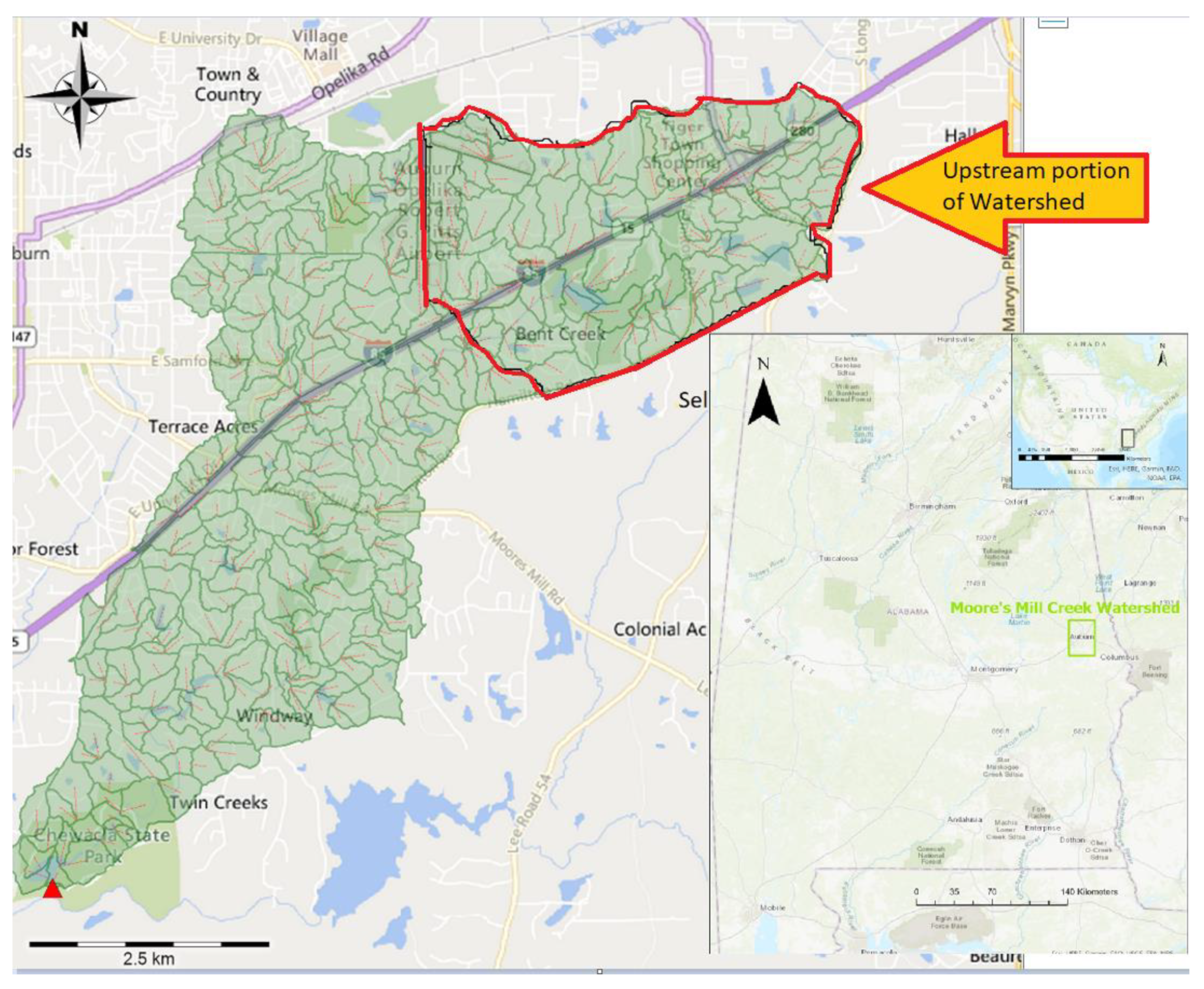
This work entailed the development of field data collection to support model simulation and calibration [27] using SWMM and WinTR-55 tools. The selected urban watershed to perform the research tasks were at the headwaters of Moore’s Mill Creek, a second-order stream located within Lee County, Alabama. The creek flows from northeast to southwest, crossing the cities of Opelika and Auburn and finishing in Chewacla State Park. The entire Moore’s Mill Creek watershed occupies an area near 30 km2, as shown in Figure 1, though the selected area is in the upper one-third (10.7 k m2) of the watershed. Moore’s Mill Creek is of environmental relevance as it is included on Alabama’s list of impaired streams for siltation [28].
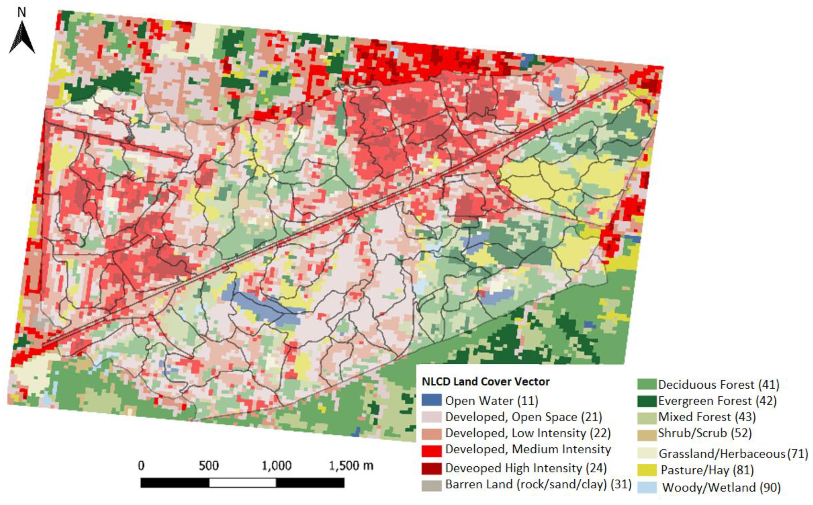
The selected research area has urban and mixed land use. Three predominant land use types are identified as “open space,” “commercial area,” and “residential area.” Using the QGIS plugin “CurveNumberGenerator” [26], the NLCD and SSURGO maps were generated. Figure 2 shows the NLCD map of the selected research area at Moore’s Mill watershed areas and the types of land use classification. Figure 3 presents the corresponding soil map from SSURGO, with the predominant Hydrologic Soil Groups being type B and the most common soil type being Pacolet sandy loam. The application of the plugin “ CurveNumberGenerator” [26] enabled the computation of a regular grid with 30 m × 30 m areas, and these areas were spatially averaged within SWMM subcatchments using a code developed in Microsoft Excel Visual Basic for Applications.
2.1. Field Work
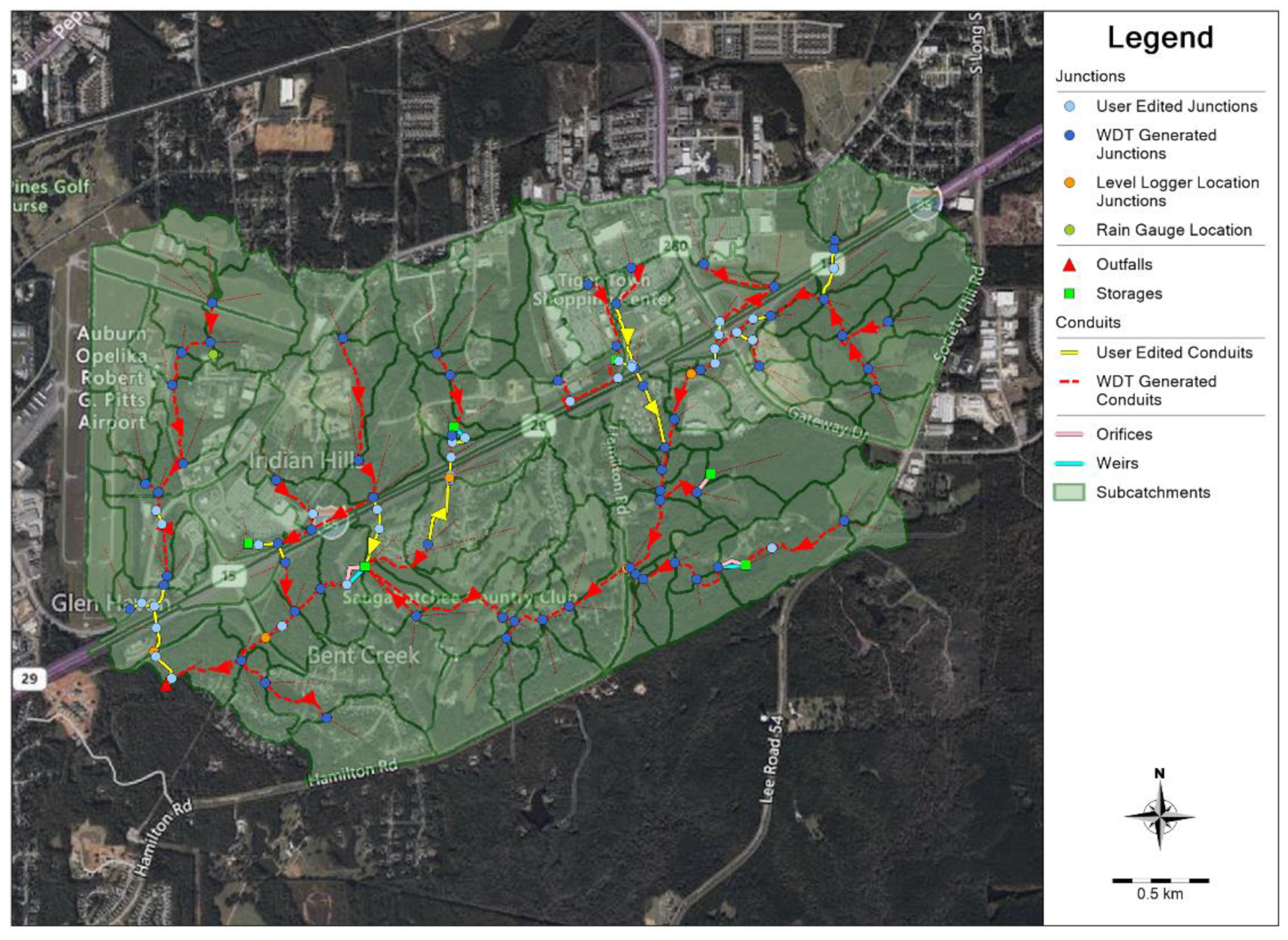
In the field investigation, five HOBO U20L 04 Water Level loggers were used to monitor the water depth at selected locations in the watershed, as is shown in Figure 4. The sensor measured and recorded the pressure with a 15 min frequency. The sensor range was 3.96 m (13 ft) with an accuracy of ±0.1% of the full scale (0.4 cm) [29]. The locations where the sensors were deployed in sub-watersheds were identified as: Capps Way; Hamilton Road; Bent Creek Road; Lakeshore Drive, and Champions Boulevard. An additional HOBO U20L 04 provided atmospheric pressure correction. The characteristics of the sub-watersheds are the following:
- Capps Way is the sub-watershed most upstream and is the headwaters of Moore’s Mill Creek. The land use is mostly comprised of forested areas, with is some ponds, low-density residential and commercial land use.
- Hamilton Road is a sub-watershed located mid-point along the stretch of Moore’s Mill Creek studied in this work. It drains a large commercial area and includes some ponds and forested areas.
- Bent Creek Road is the sub-watershed located most downstream of the studied stretch of Moore’s Mill Creek. It adds more low-density residential areas and more ponds. A dam at Hamilton Lake, which is immediately upstream of Bent Creek Road, provides peak flow attenuation during intense storms.
- Lakeshore Drive sub-watershed is a tributary watershed north of Moore’s Mill Creek, primarily with forested areas, low-density residential areas, and a pond.
- Champions Boulevard sub-watershed is another tributary north to Moore’s Mill Creek, with mostly poorly drained soils, larger fraction of impervious areas due to a regional airport and commercial areas, and absence of ponds.
Figure 4.
Sub-catchments within Moore’s Mill Creek with the location of the conduits, junctions and the sensors deployed in the field investigation.
Figure 4.
Sub-catchments within Moore’s Mill Creek with the location of the conduits, junctions and the sensors deployed in the field investigation.

A HOBO Data Logging Rain Gauge (RG3), a tipping-bucket rain gauge [30], was installed within a university property in Moore’s Mill Creek watershed to provide the rainfall data. In addition, field surveys were made to characterize the geometry of in-stream structures and channel cross-sections to improve SWMM model representations. A Global Water current meter FP211-S, with an accuracy of 0.03 m/s (0.1 ft/s), was used to measure base flows. These base flows were added in selected junctions in the SWMM model to represent the steady contributions of groundwater to Moore’s Mill base flow. That was a needed step since the aquifer components were not presented in the SWMM models, but it affected the prediction of recession limbs. Given the research goals and the SWMM model calibration focused on peak flows, the absence of an aquifer component in SWMM was not considered a key limitation of the work.
2.2. Numerical Modeling
SWMM is a semi-distributed hydrologic model based on conservation laws with robust hydraulic and water quality modeling capabilities for either event-based or continuous simulations. This research used PCSWMM (Personal Computer Storm Water Management Model), a commercial version of SWMM developed by Computational Hydraulics International (CHI). PCSWMM uses the SWMM 5 calculation engine, coupling it with pre- and post-processing tools to help in the data input and analysis tasks. These tools include the Watershed Delineation Tool (WDT) and the Sensitivity-based Radio Tuning Calibration Tool (SRTC). Digital elevation model (DEM) Data from the USDA Geospatial Gateway [31] was used in PCSWMM to delineate watersheds, provide junction elevations and develop stream transects. Storage units were transferred from the junctions manually at the open water locations. United States Geological Survey (USGS) StreamStats [32] helped to confirm the alignment of conduits obtained with PCSWMM. The transects intersecting each conduit were averaged to represent the geometries of conduits. Following Denver’s Urban Drainage and Flood Control District’s suggestion [33], the maximum flow path has not exceeded 150 m. The Manning’s roughness n for sewers was set as 0.015, and for natural channels, it was set to 0.05 based on the ASCE Manual of Practice No. 60 [34]
Once the elements in the subcatchments were adjusted, several parameters of the subcatchments were changed based on the criteria of different land use types. Manning’s roughness n for overland flow was set up based on Table 1, whereas the depression storage criteria used in the model were based on Design & Construction of Urban Stormwater Management Systems [35], where Ds was set as 2 mm for the impervious surface, and 5 mm or 8 mm for pasture and forest litter, respectively.
After all the parameters of the physical elements were set up, the infiltration method was selected as the curve number method. Assigning CN values for subcatchments is time-consuming, considering spatial averaging and the uncertainties associated with land use and soil characteristics. The Fully Composite CN approach simplifies the SWMM modeling setup as there would be no need to average CN only for the pervious areas. However, some potential limitation is the underestimation of the total runoff, as pointed out by Ormsbee et al. [37]. The proposed approach of defining whether an area is impervious based on the CN threshold value can potentially avoid runoff underestimation while retaining model setup simplicity.
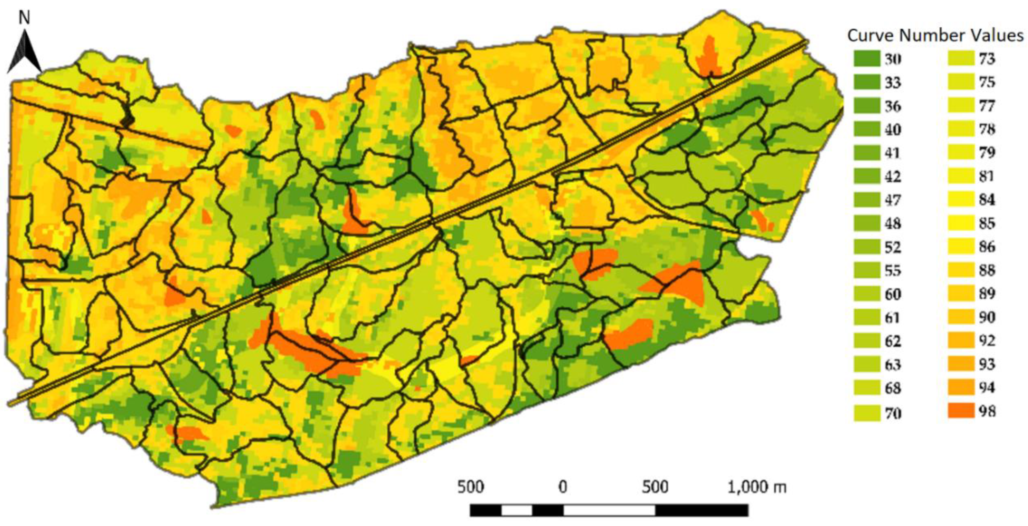
Shapefile for the subcatchments layer generated in PCSWMM was imported into the geospatial software Quantum Geographic Information System (QGIS) through the plugin CurveNumberGenerator [26]. The algorithm in this plugin uses the NLCD [21] and SSURGO [22] as reference tables to automatically compute CN values for a 30 m × 30 m regular grid, as shown in Figure 5. Subsequently, a spreadsheet computed spatial average values for CN values considering the values within a given subcatchment.
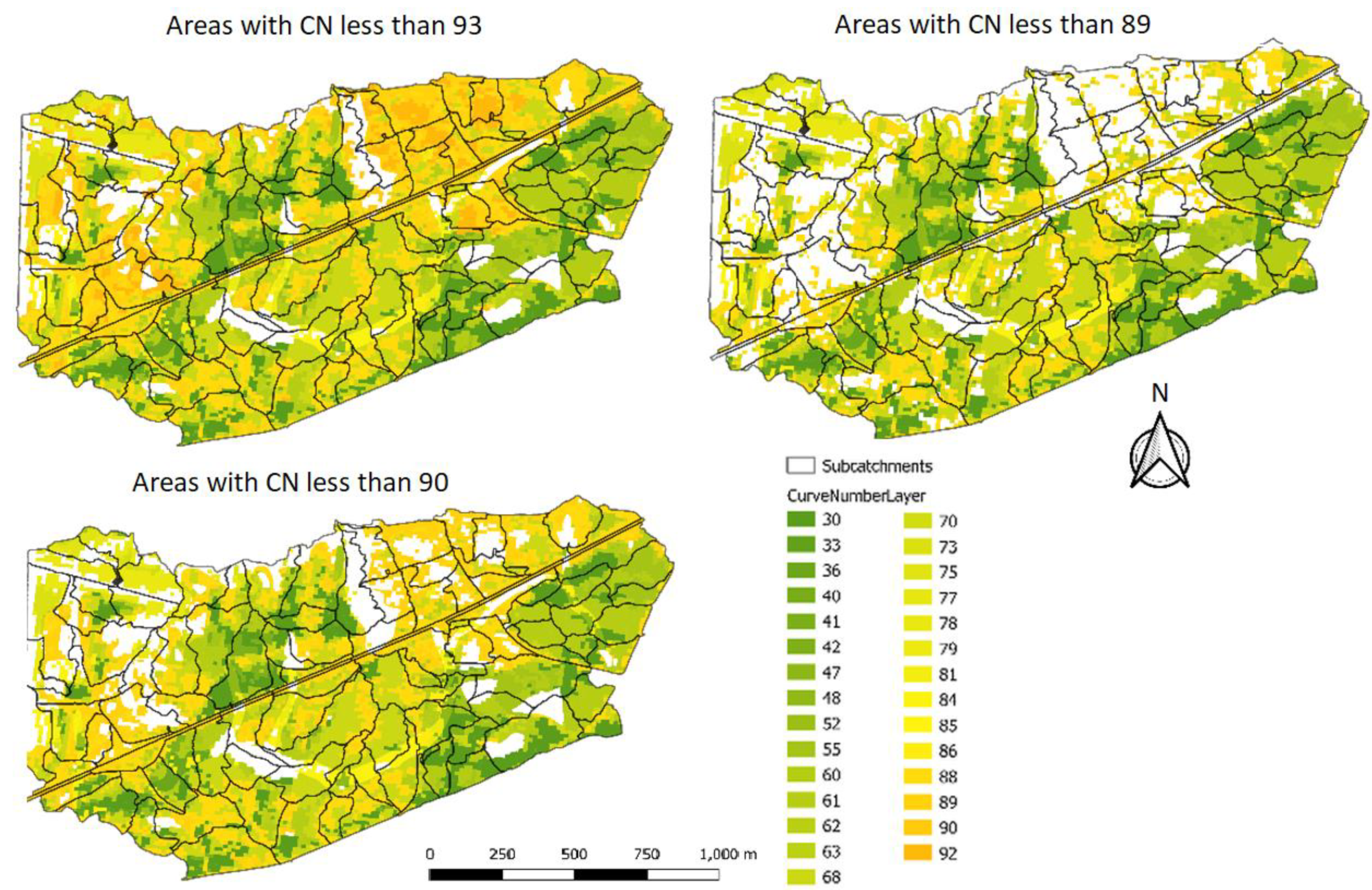
For the CN Cut-off approach, the generated CN layer was selected based on a pre-selected value for CN Cut-off to generate a new CN layer. This means that areas with CN values above a certain threshold, considered either 93, 90, or 89, were assumed impervious. The CN values below the threshold would be averaged and assigned to a given SWMM subcatchment. The selected thresholds CN Cut-off were based on the resulting number of features (i.e., regular grid cells) considered pervious in the subcatchments. Table 2 shows that the Fully Composite had 100% features or 2430 grid cells in the CN layer. As the CN threshold dropped, fewer cells were considered pervious, as shown in Table 2. The CN threshold values of 93, 90, and 89 created significant variations between the number of pervious features to enable a useful comparison between the CN Cut-off method with the Fully Composite approach (Figure 6).
A model calibration process was used to improve the model performance, and this was performed by applying PCSWMM’s SRTC tool. In this study, several parameters were considered, but the most relevant were depression storage and Manning’s roughness for impervious and pervious areas. These parameters were calibrated by considering past research [35,36]. Other parameters, such as subcatchments slope and subcatchment drying time, were also considered in the calibration process. Notably particularly, CN values were not calibrated as these values were adopted from the calculations performed with the QGIS plugin and spatial averaging, diverging from related SWMM investigations [38,39] that applied the CN method. Upon comparing field collected data and initial modeling results, it was determined that the modeling results closer to the observations were based on the CN Cut-off at 90. Thus, the calibration was performed considering the CN Cut-off threshold of 90, and all the calibration setup was applied for the other SWMM models based on Fully Composite and the CN Cut-off values.
A warm-up period was also applied when running the calibration process to reduce the model dependence on the initial conditions. The accuracy of the model was based on its ability to compute peak depth was plotted as compared with field measurements. In addition, and following [40,41], other statistics can be used to determine the adequacy of the modeling effort. If daily, monthly, or the annual coefficient of determination (R2) > 0.6, Nash-Sutcliffe efficiency (NSE) is larger than 0.5, and percent bias (PBIAS) less or equal to ±15% for watershed-scale models, the model performance can be judged “satisfactory.”
As pointed out earlier, WinTR-55 is a hydrologic model designed for small watersheds by the Natural Resources Conservation Service (NRCS) [3]. Among the differences between WinTR-55 and SWMM is that the former is a single-event model tool. WinTR-55 is used to analyze watersheds less or equal to 10 subcatchments and can calculate the peak flows from design storms with different flood return periods. The model input includes the characteristics of watersheds, including a weighed CN value for the entire subcatchment, reach geometry, design storms, and other data sources [3].
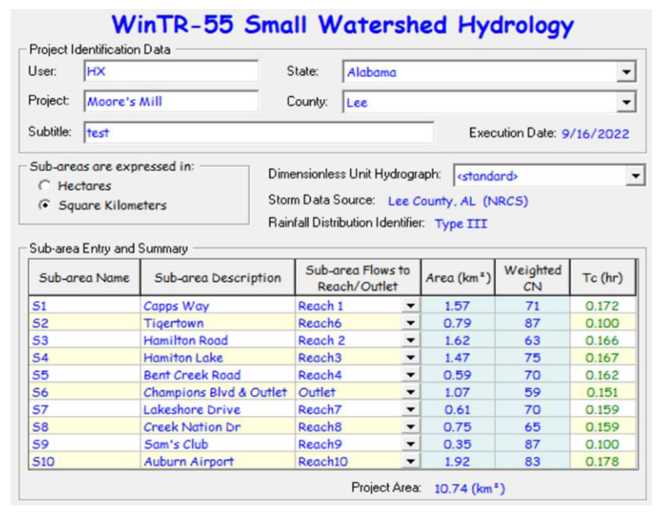
Because the maximum number of subcatchments in a WinTR-55 model is 10, separate SWMM 5 models using ten subcatchments to represent Moore’s Mill Creek watershed were constructed. This model with fewer subcatchments used the same calibration settings as the previous SWMM models. The comparison was made using synthetic rainfall distributions at different design rainfall return periods. The rain events for SWMM 5 and WinTR-55 were Type III 24 h long rainfall events for 1-year, 2-year, and 5-year rainfall return periods. Finally, WinTR-55 primary results are flow rate hydrographs, and these are the results that were compared with SWMM 5 predictions. Figure 7 presents the information on the subcatchments used in the WinTR-55 model.
3. Results and Discussion
3.1. Watershed Properties and Resulting CN Values
The areas, imperviousness, and CN values of the five sub-watersheds that corresponded to the fieldwork data collection are shown in Table 3 and the locations for these are shown in Figure 4. As pointed out earlier, areas with CN values at or above the Cut-off value were used as a surrogate to determine whether the area was impervious. Results in Table 3 indicate that the CN Cut-off at 90 yielded values for percent imperviousness in the sub-watersheds closest to the corresponding values obtained by StreamStats [42] which in turn used data from NLCD dataset.
As shown in Table 4, the average CN values of each sub-watershed decreased from the Fully Composite CN approach to the CN Cut-off at 89. This was expected given that the Fully Composite averages CN values from all areas, including impervious areas with high CN values. Conversely, as we moved from the Fully Composite into the lowest CN Cut-off value approaches, the average CN for the pervious areas increased, indicating more infiltration potential for the pervious fraction.
3.2. Flow Depth Hydrograph Results and Discussion
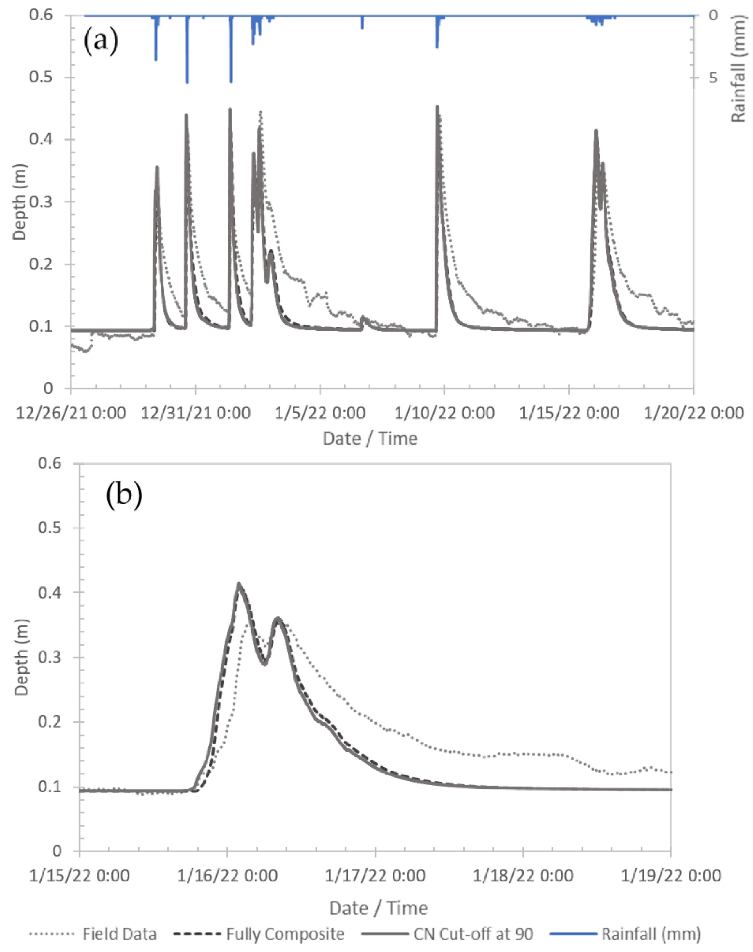
Figure 8 presents observed flow depths hydrographs for the Bent Creek Road sub-watershed, with corresponding SWMM model predictions. The presented results considered two different CN approaches: Fully Composite and CN Cut-off at 90. From a visual inspection, both CN calculation approaches have comparable performance in describing the peak flow, with a higher tendency to predict higher peak flow depths than observed values. The recession limb modeling results are not well predicted. As pointed, the model was developed without using SWMM aquifer objects, and the faster drop in the modeled depth following the rain events is attributed to the lack of a groundwater exfiltration.
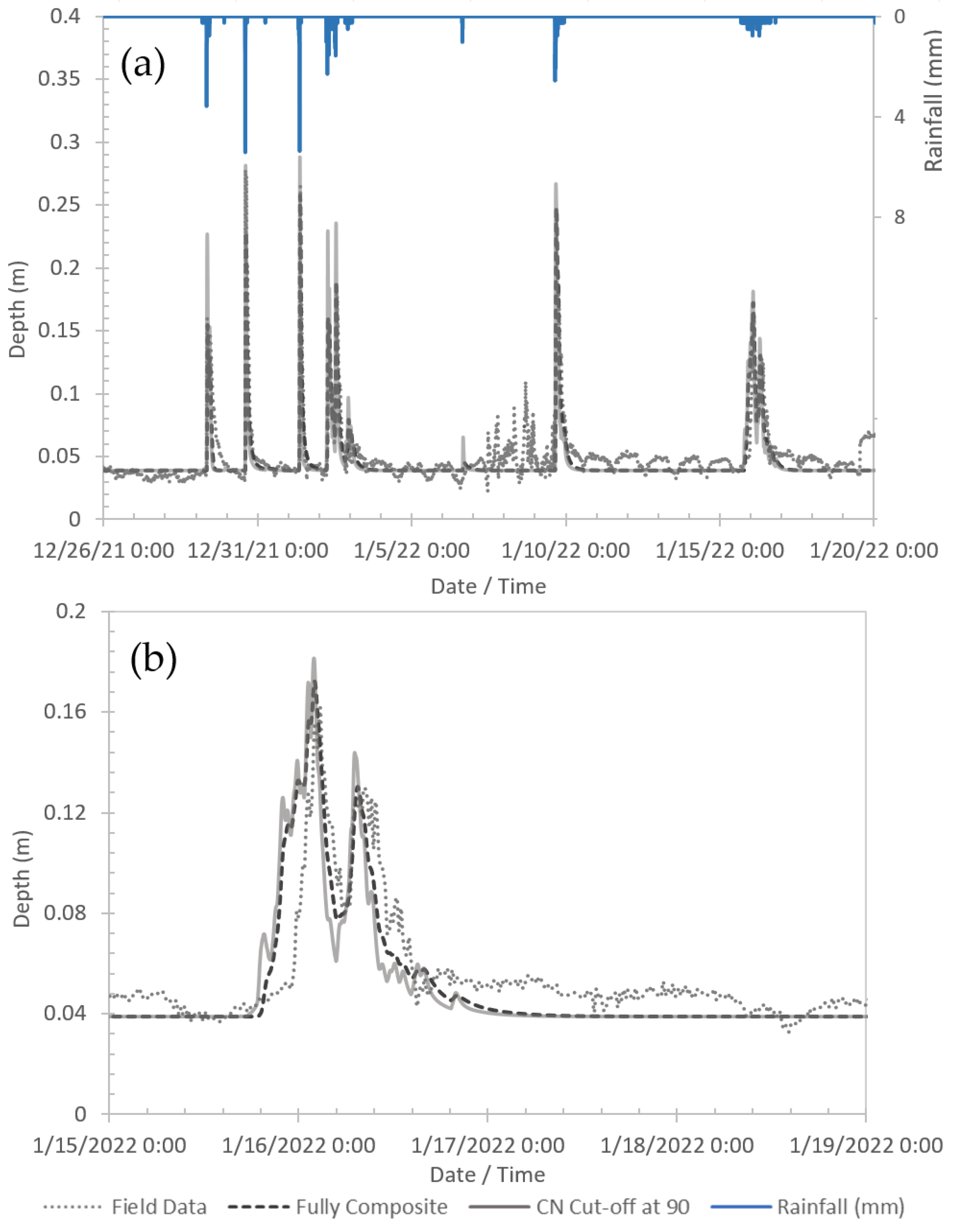
Similar results are shown in Figure 9 for the Champions Blvd sub-watershed. However, there is a slight overestimation of the flow depth yielded by the CN Cut-off method. Interestingly, the discrepancy observed with the recession limb is less pronounced at this location, which is attributed to the higher level of imperviousness and overall large CN values in this sub-watershed. The results shown in both Figure 8 and Figure 9 indicate that there was a mismatch between the modeled and observed times for the rise of the depth hydrographs. Two potential causes could explain differences. One is the difference between the actual rainfall in the sub-watersheds and the one measured in the study. Another possibility is related to the SWMM 5 option “subarea routing”. In this study, all subareas were routed directly to the outlet of the subcatchment, and if a fraction of the flows were routed to pervious areas, the time to achieve the peak could be closed than the observations.
3.3. Peak Flow Depth Results and Discussion
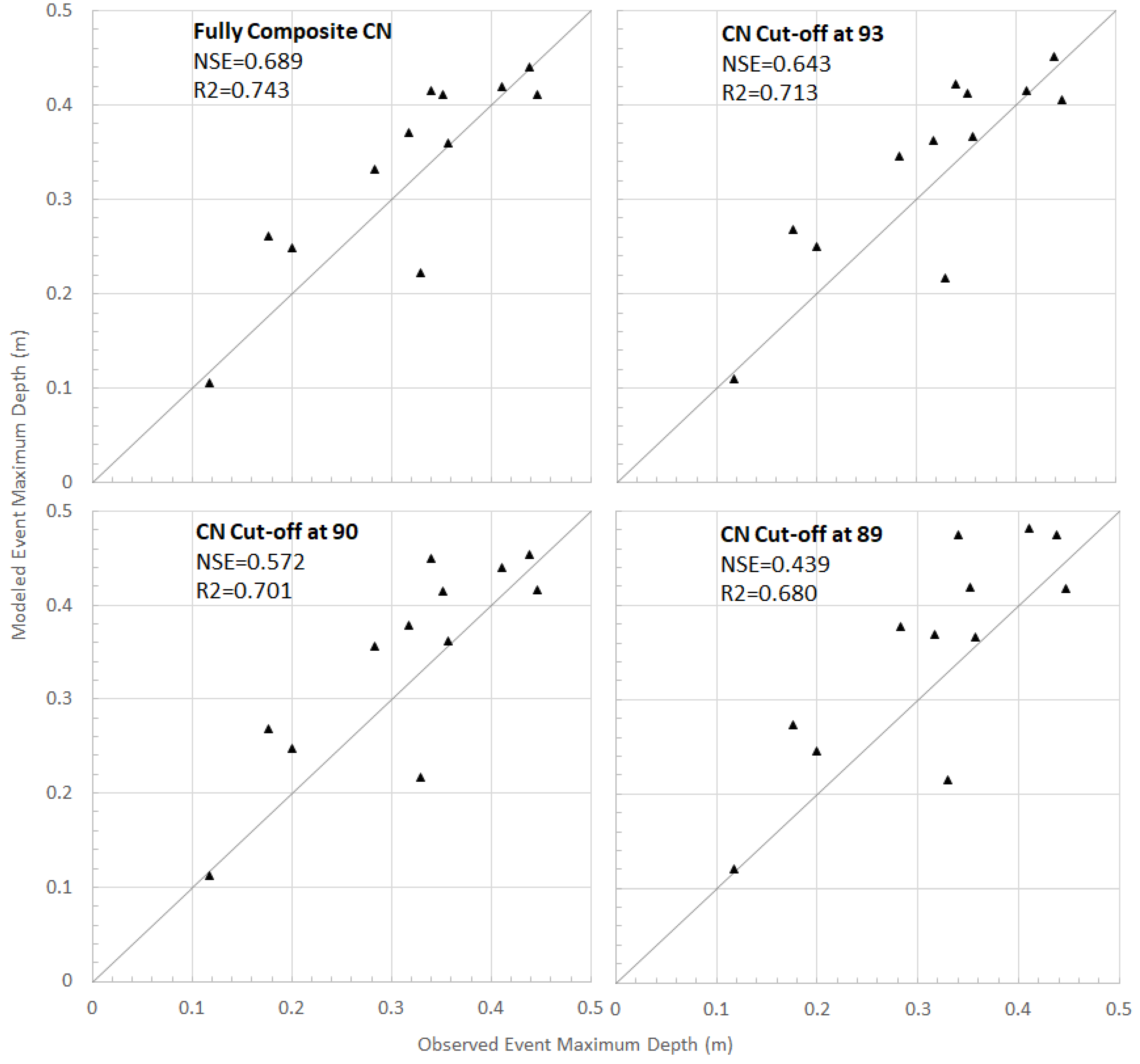
As pointed out, Fully Composite CN values for watersheds were comparatively higher because they averaged the CN from all types of land use in the SWMM subcatchments while assuming zero impervious areas. As the Cut-off value decreased, the averaged CN decreased, but the impervious fraction increased. It was uncertain how these conditions would impact the peak flow depth predicted by these different approaches to represent CN. The results presented in Figure 10 and Figure 11 compare the peak flow depth observed in the streams versus the corresponding modeled values for the Bent Creek Road and Champions Blvd. sub-watersheds, respectively.
As is indicated in Figure 10 and Figure 11, the points in the graph tend to migrate to the left, which means that the modeled peak predictions increase with smaller CN Cut-off values. As indicated in [4], it appears that the lowest CN Cut-off created unrealistically large fraction of impervious areas, which systematically yielded larger predicted peak flow depths. Results for these two sub-watersheds indicated that the NSE and R2 values for the predicted vs. modeled peak flow depth were slightly better for the Fully Composite approach. However, as shown in Table 5 (NSE results) and Table 6 (R2 results), on average, the peak flow depth statistics results are better for the CN Cut-off values of 90 or 93 when considering all five sub-watersheds.
Table 5 also supports the conclusion that the worst NSE results were observed in the Lakeshore Drive sub-watershed, which is the sub-watershed with the lowest average CN value. Moreover, the model performance measured in terms of NSE for Champions Boulevard, the sub-watershed with the highest CN value, because steadily worse in models with larger CN Cut-off values. Except for the Champions Boulevard. sub-watershed, the NSE performance was consistently higher for the CN-Cut-off at 90. The R2 statistic, shown in Table 6, was less sensitive to the different approaches to compute CN in the model results, with the CN Cut-off values of 90 or 93 again outperforming the other alternatives.
3.4. Flow Hydrograph Comparison between WinTR-55 and SWMM 5 Models
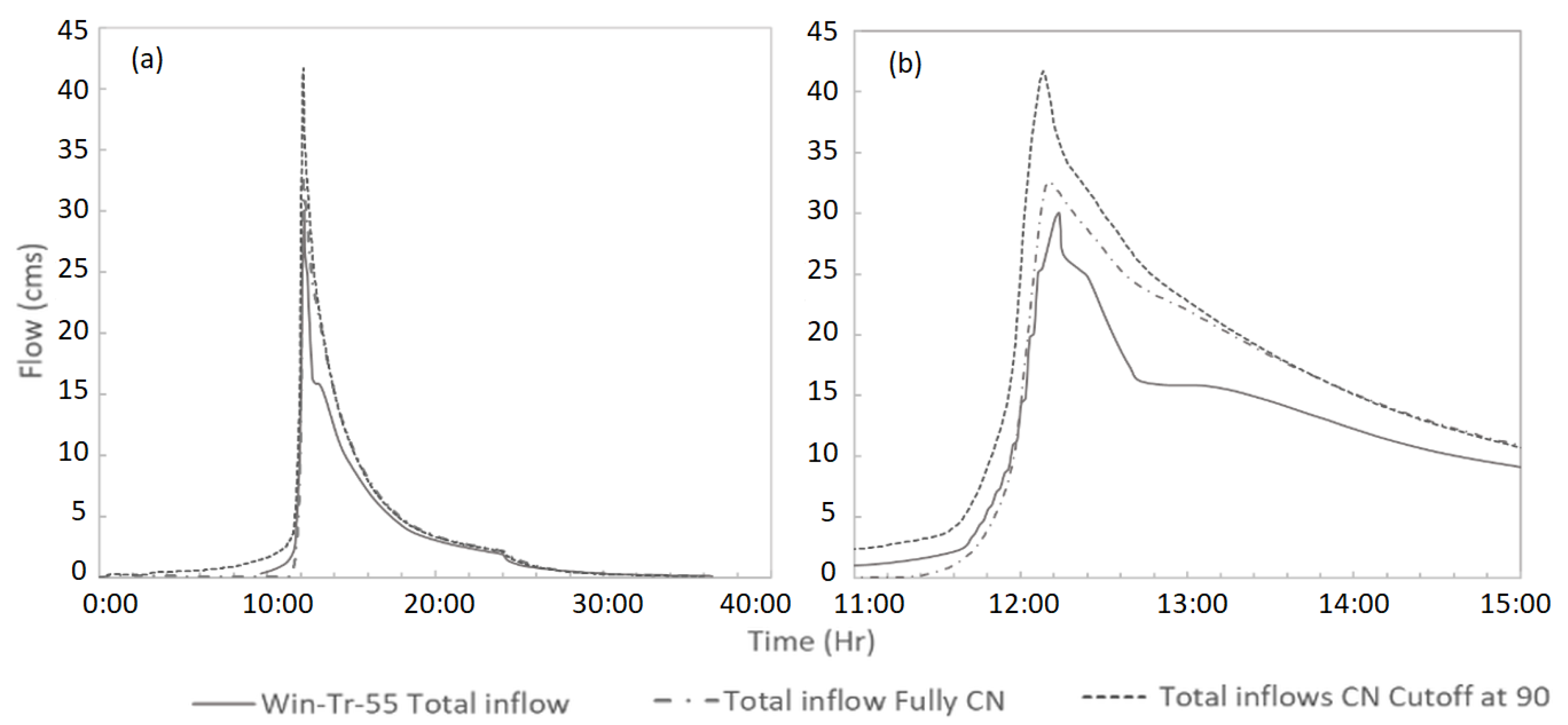
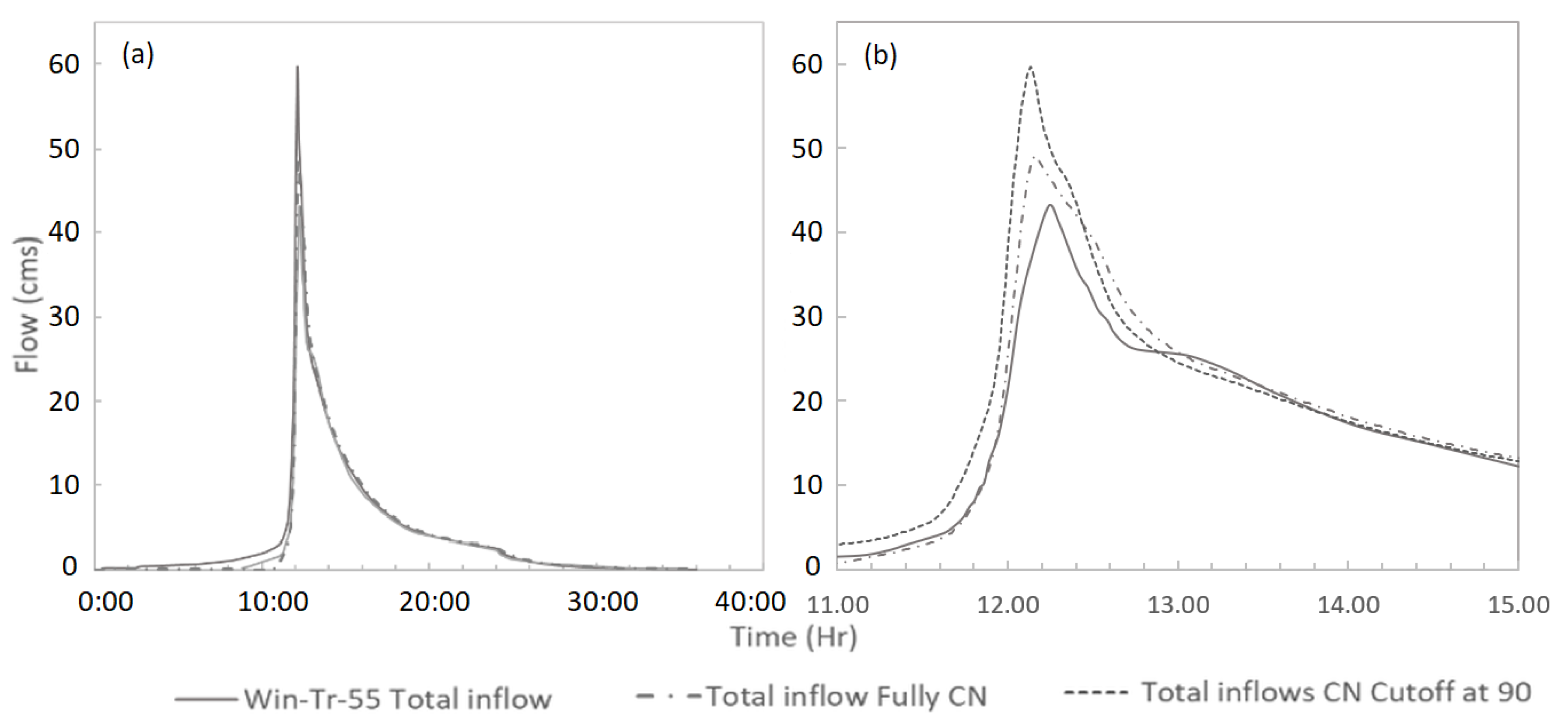
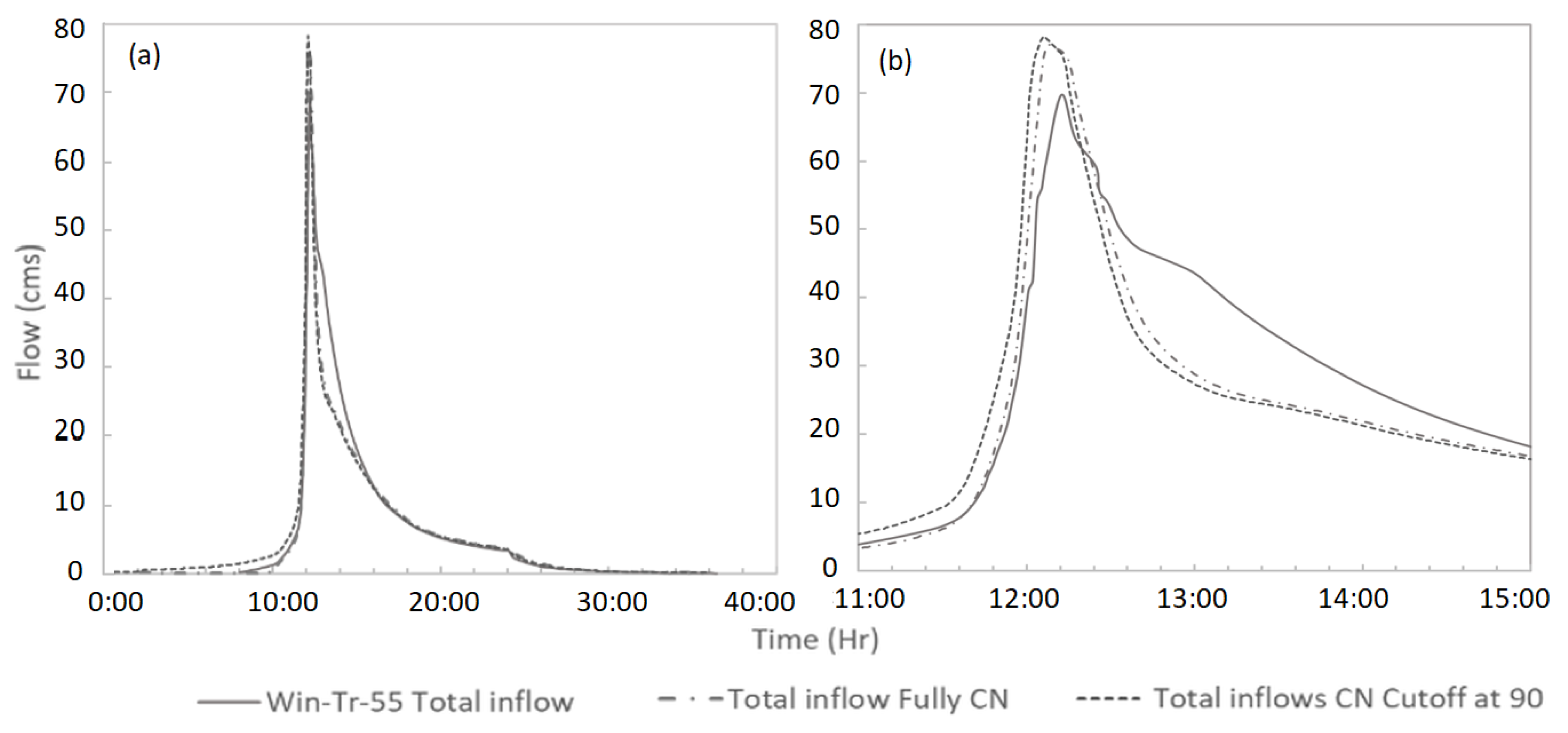
SWMM and WinTR-55 modeling results were compared for the selected research area at Moore’s Mill Creek watershed with three Type III design storms. This comparison considered only the Fully Composite CN approach, which follows the same CN computation approach of WinTR-55, and the CN Cut-off at 90. The flow rate hydrographs for the 1, 2, and 5-year return periods are presented in Figure 12, Figure 13 and Figure 14, respectively. A few observations can be drawn from analyzing these results:
- As would be anticipated, SWMM modeling results from the Fully Composite approach are consistently closer to the flow hydrographs yielded by WinTR-55. However, this agreement decreased with the more intense rain events.
- WinTR-55 peak flow results were consistently smaller than SWMM modeling results.
- The CN Cut-off 90 and the Fully Composite approach agreement increased for higher intensity rain events. However, the CN Cut-off consistently had higher peak flows than the Fully Composite approach.
- Finally, the relative discrepancy between the model results decreased steadily with larger intensity rain events.
Figure 12.
(a) Flow hydrograph for Moore’s Mill watershed yielded by WinTR-55 and two SWMM models of a Type III 24 h long, 1 yr return period rain. (b) Detailed view of the peak flows.
Figure 12.
(a) Flow hydrograph for Moore’s Mill watershed yielded by WinTR-55 and two SWMM models of a Type III 24 h long, 1 yr return period rain. (b) Detailed view of the peak flows.

Figure 13.
(a) Flow hydrograph for Moore’s Mill watershed yielded by WinTR-55 and two SWMM models of a Type III 24 h long, 2 yr return period rain. (b) Detailed view of the peak flows.
Figure 13.
(a) Flow hydrograph for Moore’s Mill watershed yielded by WinTR-55 and two SWMM models of a Type III 24 h long, 2 yr return period rain. (b) Detailed view of the peak flows.

Figure 14.
(a) Flow hydrograph for Moore’s Mill watershed yielded by WinTR-55 and two SWMM models of a Type III 24 h long, 5 yr return period rain. (b) Detailed view of the peak flows.
Figure 14.
(a) Flow hydrograph for Moore’s Mill watershed yielded by WinTR-55 and two SWMM models of a Type III 24 h long, 5 yr return period rain. (b) Detailed view of the peak flows.

3.5. Summary of the Findings and Discussion
The application of CN in various hydrologic modeling context is widespread, and involves many models such as SWMM, HEC-HMS, WinTR-55, among others. Various modeling tools assume that a CN-modeled infiltration will occur over the entirety of subcatchments. However, SWMM models can assume that subcatchments have impervious and pervious fractions, with the infiltration occurring on the latter. Results were obtained through an evaluation of the effects of using increasingly large impervious fractions through lower CN Cut-off numbers.
One important observation is that the results with lower CN Cut-off yielded consistently larger flow hydrographs compared to the Fully Composite approach with all areas being pervious. This agrees with the observations in Section 4.5.4 on [4] and can support to other modelers performing studies using SWMM and CN-based infiltration. The Fully Composite was considered the best modeling approach in terms of NSE and R2 results for the Champions Blvd. sub-watershed, the one with largest average CN values. However, CN Cut-off 93 modeling results were consistently good for all watersheds. This indicate that CN could indeed be a surrogate for imperviousness for both SWMM and other modeling tools. This observation, however, will need to be further assessed for other watersheds and hydrological conditions.
A final interesting observation came from the comparison between SWMM 5 and WinTR-55 regarding the predicted flow hydrographs. Despite the efforts to create a SWMM 5 model set up as close as possible to the WinTR-55 model, peak flow rates were consistently higher in SWMM 5 results. This difference was smaller for the Fully Composite SWMM results, which is expected since this is the approach used in WinTR-55. However, differences were still significant for the rain events with smaller return period. This indicates that an analyst must use careful judgement when comparing results yielded by different modeling tools, albeit using the same CN values, rainfall, and model parameters.
4. Conclusions and Recommendations for Future Work
Hydrologic models have been widely applied to design and manage water resources, including stormwater management in urban watersheds. The accuracy and quality of data input are of paramount importance so that model predictions are helpful and represent well the local hydrology. Infiltration is a critical component of hydrologic models. Due to its simplicity and data availability, the Curve Number infiltration model is one of the most adopted methodologies to compute infiltration abstractions. SWMM 5 adopts CN as an option to compute infiltration, but the approaches to create models can differ in terms of whether impervious fractions should be used or not. This work assumed CN as the criteria to define whether an area is impervious, and the studied the impacts in the modeling results of using various CN thresholds.
In general, the CN Cut-off value of 93 and 90 presented the best results for the sub-watersheds with average CN values in the range of mid-60 to mid-70. The Fully Composite approach, which averaged CN values for all areas in a subcatchment, performed best for the sub-watershed with the highest level of imperviousness and largest CN values. While a relevant observation, further studies are planned in other areas within Moore’s Mill watershed to confirm these observations. Other similar investigations should also be performed in other hydrological conditions to assess whether CN could be a surrogate for imperviousness in modeling subcatchments.
A comparison between WinTR-55 model results and SWMM indicated that the latter yielded flow rate hydrographs consistently larger than WinTR-55 predictions. Such discrepancy decreased for the SWMM 5 Fully Composite model results and for rain events with larger return periods. Nevertheless, this comparison should also be considered in subsequent studies for other watersheds and other hydrological conditions. A comparison between SWMM 5 and other hydrological models using CN is potentially an area to be explored in future investigations. Finally, it is planned to include the effects of groundwater in the SWMM modeling efforts in the future stages of this research.
Author Contributions
Conceptualization, H.X. and J.G.V.; methodology, H.X. and J.G.V.; software, H.X.; formal analysis, H.X. and J.G.V.; investigation, H.X. and J.G.V.; writing—original draft preparation, H.X.; writing—review and editing, J.G.V. All authors have read and agreed to the published version of the manuscript.
Funding
This research received no external funding.
Data Availability Statement
All the data that support the findings of this study are available from the corresponding author upon reasonable request.
Acknowledgments
The authors would like to acknowledge the CHI (Computational Hydraulic International) for granting the Educational License of PCSWMM (Personal Computer Storm Water Management Model).
Conflicts of Interest
The authors declare no conflict of interest.
References
- Feldman, A.D. Hydrologic Modeling System HEC-HMS Technical Reference Manual; U.S. Army Corps of Engineers Hydrologic Engineering Center, HEC: Davis, CA, USA, 2000; pp. 1–3. [Google Scholar]
- Rossman, L.A. Storm Water Management Model User’s Manual Version 5.1; U.S. Environmental Protection Agency, National Risk Management Research Laboratory Office of Research and Development: Cincinnati, OH, USA, 2015; pp. 12–13. [Google Scholar]
- NRCS. Small Watershed Hydrology WinTR-55 User Guide; United States Department of Agriculture: Washington, DC, USA, 2009. [Google Scholar]
- Rossman, L.A. Storm Water Management Model Reference Manual; Volume I—Hydrology (Revised); National Risk Management Laboratory Office of Research and Development U.S. Environmental Protection Agency: Cincinnati, OH, USA, 2016; pp. 86–87. [Google Scholar]
- Horton, R.E. The Role of Infiltration in the Hydrologic Cycle. Trans. Am. Geophys. Union 1933, 14, 446–460. [Google Scholar] [CrossRef]
- Green, W.H.; Ampt, G.A. Studies on Soil Physics, 1. The Flow of Air and Water Through Soils. J. Agric. Sci. 1911, 4, 11–24. [Google Scholar]
- NRCS. Urban Hydrology for Small Watersheds: TR-55; U.S. Department of Agriculture: Washington, DC, USA, 1986. [Google Scholar]
- Dao, D.A.; Kim, D.; Tran, D.H.H. Estimation of rainfall threshold for flood warning for small urban watersheds based on the 1D–2D drainage model simulation. Stoch. Environ. Res. Risk Assess. 2021, 36, 735–752. [Google Scholar] [CrossRef]
- Custodio, D.A.; Ghisi, E. Impact of residential rainwater harvesting on stormwater runoff. J. Environ. Manag. 2022, 326, 116814. [Google Scholar] [CrossRef] [PubMed]
- Prokešová, R.; Horáčková, Š.; Snopková, Z. Surface runoff response to long-term land use changes: Spatial rearrangement of runoff-generating areas reveals a shift in flash flood drivers. Sci. Total Environ. 2021, 815, 151591. [Google Scholar] [CrossRef] [PubMed]
- Barbero, G.; Costabile, P.; Costanzo, C.; Ferraro, D.; Petaccia, G. 2D hydrodynamic approach supporting evaluations of hydrological response in small watersheds: Implications for lag time estimation. J. Hydrol. 2022, 610, 127870. [Google Scholar] [CrossRef]
- Dao, D.A.; Kim, D.; Kim, S.; Park, J. Determination of flood-inducing rainfall and runoff for highly urbanized area based on high-resolution radar-gauge composite rainfall data and flooded area GIS data. J. Hydrol. 2020, 584, 124704. [Google Scholar] [CrossRef]
- Garen, D.C.; Moore, D.S. Curve Number Hydrology in Water Quality Modeling: Uses, Abuses, and Future Directions. J. Am. Water Resour. Assoc. 2005, 41, 377–378. [Google Scholar] [CrossRef]
- Praskievicz, S.; Chang, H. A review of hydrological modelling of basin-scale climate change and urban development impacts. Prog. Phys. Geogr. 2009, 33, 650–671. [Google Scholar] [CrossRef]
- Yan, H.; Edwards, F.G. Effects of Land Use Change on Hydrologic Response at a Watershed Scale, Arkansas. J. Hydrol. Eng. 2013, 18, 1779–1785. [Google Scholar] [CrossRef]
- Hawkins, R.H.; Ward, T.J.; Woodward, D.E.; Mullem, J.A.V. Curve Number Hydrology; Environmental and Water Resources Institute (EWRI) of the American Society of Civil Engineers: Reston, VA, USA, 2009. [Google Scholar]
- Hawkins, R.H.; Theurer, F.D.; Rezaeianzadeh, M. Understanding the Basis of the Curve Number Method for Watershed Models and TMDLs. J. Hydrol. Eng. 2019, 24, 06019003. [Google Scholar] [CrossRef]
- Galbetti, M.V.; Zuffo, A.C.; Shinma, T.A.; Boulomytis, V.T.G.; Imteaz, M. Evaluation of the tabulated, NEH4, least squares and asymptotic fitting methods for the CN estimation of urban watersheds. Urban Water J. 2022, 19, 244–255. [Google Scholar] [CrossRef]
- Bartlett MSParolari, A.J.; McDonnell, J.J.; Porporato, A. Beyond the SCS-CN method: A theoretical frameworkfor spatially lumped rainfall-runoff response. Water Resour. Res. 2016, 52, 4608–4627. [Google Scholar] [CrossRef] [Green Version]
- Hawkins, R.H. The importance of accurate curve numbers in the estimation of storm runoff. Water Resour. Bull. Am. Water Resour. Assoc. 1975, 11, 887–890. [Google Scholar] [CrossRef]
- USGS. National Land Cover Database (NLCD) 2019 Products (version 2.0, June 2021); U.S. Geological Survey data release: Reston, VA, USA, 2021. [Google Scholar] [CrossRef]
- USDA. Soil Survey Geographic Database (SSURGO). 2015. Available online: https://data.nal.usda.gov/dataset/soil-survey-geographic-database-ssurgo (accessed on 1 September 2022).
- Schoenfelder, C.; Kacvinsky, G.; Rossman, L. Open SWMM: Curve Number Assignment. 2007. Available online: https://www.openswmm.org/Topic/3481/curve-number-assignment (accessed on 10 October 2022).
- Zhang, G.; Dickinson, R.; Rovak, G.; Rossman, L. Open SWMM: Runoff Calculation Using Curve Number. 2007. Available online: https://www.openswmm.org/Topic/3584/runoff-calculation-using-curve-number (accessed on 10 October 2022).
- Numan, U.; Dickinson, R. Curve Numbers vs. % Impervious. 2022. Available online: https://www.openswmm.org/Topic/32629/curve-numbers-vs-impervious (accessed on 10 October 2022).
- Siddiqui, A.R. Curve Number Generator: A QGIS Plugin to Generate Curve Number Layer from Land Use and Soil. 2020. Available online: https://github.com/ar-siddiqui/curve_number_generator (accessed on 1 May 2022).
- James, W. Rules for Responsible Modeling; Computional Hydraulics International (CHI): Guelph, ON, Canada, 2005. [Google Scholar]
- Acer Engineering LLC. Moore’s Mill Creek Watershed Management Plan, Lee County, Alabama; Acer Engineering LLC: Raleigh, NC, USA, 2008. [Google Scholar]
- HOBO® Data Logger. HOBO® U20L Water Level Logger (U20L-0x) Manual; Onset Computer Corperation: Bourne, MA, USA, 2022; Available online: https://www.onsetcomp.com/datasheet/U20L-04 (accessed on 1 September 2021).
- HOBO Data Logging Rain Gauge (RG3 and RG3-M) Manual. Corporation, O.C., Ed. 2005–2018. Available online: https://www.onsetcomp.com/files/manual_pdfs/10241-M%20MAN-RG3%20and%20RG3-M.pdf (accessed on 1 September 2021).
- USDA. USDA Geospatial Data Gateway (GDG). Available online: https://datagateway.nrcs.usda.gov/ (accessed on 1 September 2021).
- Ries, K.G.; Guthrie, J.D.; Rea, A.H.; Steeves, P.A.; Stewart, D.W. StreamStats: A Water Resources Web Application; USGS Publicaitons Warehouse: Reston, VA, USA, 2008. [Google Scholar]
- UDFCD. Runoff. In Drainage Criteria Manual; Urban Drainage and Flood Control District: Dever, CO, USA, 2007; Chapter 5. [Google Scholar]
- ASCE. Gravity Sanitary Sewer Design and Construction; ASCE: New York, NY, USA, 1982. [Google Scholar]
- ASCE. Design & Construction of Urban Stormwater Management Systems; ASCE: New York, NY, USA, 1992. [Google Scholar]
- McCuen, R.E.A. Hydrology; Federal Highway Administration: Washington, DC, USA, 1996. [Google Scholar]
- Ormsbee, L.; Hoagland, S.; Peterson, K. Limitations of TR-55 Curve Numbers for Urban Development Applications: Critical Review and Potential Strategies for Moving Forward. J. Hydrol. Eng. 2020, 25, 02520001. [Google Scholar] [CrossRef]
- Alfredo, K.; Montalto, F.; Goldstein, A. Observed and Modeled Performances of Prototype Green Roof Test Plots Subjected to Simulated Low- and High-Intensity Precipitations in a Laboratory Experiment. J. Hydrol. Eng. 2010, 15, 444–457. [Google Scholar] [CrossRef]
- Swathi, V.; Raju, K.S.; Varma, M.R.R.; Veena, S.S. Automatic calibration of SWMM using NSGA-III and the effects of delineation scale on an urban catchment. J. Hydroinform. 2019, 21, 781–797. [Google Scholar] [CrossRef]
- Moriasi, D.N.; Arnold, J.G.; Liew, M.W.V.; Bingner, R.L.; Harmel, R.D.; Veith, T.L. Model Evaluation Guidelines for Systematic Quantification of Accuracy in Watershed Simulations. Am. Soc. Agric. Biol. Eng. 2007, 50, 885–900. [Google Scholar]
- Moriasi, D.N.; Gitau, M.W.; Pai, N.; Daggupati, P. Hydrologic and Water Quality Models: Performance Measures and Evaluation Criteria. Am. Soc. Agric. Biol. Eng. 2015, 58, 1763–1785. [Google Scholar] [CrossRef]
- U.S. Geological Survey. The StreamStats Program. 2019. Available online: https://streamstats.usgs.gov/ss/ (accessed on 1 August 2022).
Figure 1.
Moore’s Mill Creek watershed, located in east Alabama, USA. The area selected for this research is delineated in red.
Figure 1.
Moore’s Mill Creek watershed, located in east Alabama, USA. The area selected for this research is delineated in red.

Figure 2.
NLCD Land Cover map of selected research area at the Moore’s Mill Creek watershed.

Figure 3.
SSURGO Soil Layer map of selected research area at the Moore’s Mill Creek watershed.

Figure 5.
Curve number values within Moore’s Mill Creek watershed were calculated using the CurveNumberGenerator plugin [26] within QGIS.
Figure 5.
Curve number values within Moore’s Mill Creek watershed were calculated using the CurveNumberGenerator plugin [26] within QGIS.

Figure 6.
CN Cut-off maps for all thresholds. Notice the increase in white areas corresponding to impervious areas as the CN Cut-off value decreases.
Figure 6.
CN Cut-off maps for all thresholds. Notice the increase in white areas corresponding to impervious areas as the CN Cut-off value decreases.

Figure 7.
WinTR-55 screen with the data for the modeling of Moore’s Mill Creek watershed.

Figure 8.
(a) Bent Creek Road depth hydrograph and hyetograph with corresponding modeling results; (b) Detail of the depth hydrograph for the rain event on 16 January 2022.
Figure 8.
(a) Bent Creek Road depth hydrograph and hyetograph with corresponding modeling results; (b) Detail of the depth hydrograph for the rain event on 16 January 2022.

Figure 9.
(a) Champions Blvd depth hydrograph and hyetograph with corresponding modeling results; (b) Detail of the depth hydrograph for the rain event on 16 January 2022.
Figure 9.
(a) Champions Blvd depth hydrograph and hyetograph with corresponding modeling results; (b) Detail of the depth hydrograph for the rain event on 16 January 2022.

Figure 10.
Bent Creek Rd. peak flow depth comparison between observed and modeled results.

Figure 11.
Champions Blvd peak flow depth comparison between observed and modeled results.


Table 1.
Adopted Manning’s n for overland flow [36].
Table 1.
Adopted Manning’s n for overland flow [36].
| Surface | Manning’s n |
|---|---|
| Paved areas | 0.011 |
| Short prairie | 0.15 |
| Dense grass | 0.24 |
| Light wood underbrush | 0.4 |
| Dense wood underbrush | 0.8 |
Table 2.
Threshold values selection criteria of CN Cut-off approach (Bold values in shading lines correspond to the conditions adopted in the SWMM models).
Table 2.
Threshold values selection criteria of CN Cut-off approach (Bold values in shading lines correspond to the conditions adopted in the SWMM models).
| Method | No. of Pervious Features | No. of Impervious Features | Percent of Pervious Features |
|---|---|---|---|
| Fully Composite | 2430 | 0 | 100.0 |
| CN ≤ 98 | 2308 | 122 | 95.0 |
| 94 < CN < 98 | 2308 | 122 | 95.0 |
| CN < 93 | 2097 | 333 | 86.3 |
| 91 < CN < 92 | 1969 | 461 | 81.0 |
| CN < 90 | 1886 | 544 | 77.6 |
| CN < 89 | 1595 | 835 | 65.6 |
| CN < 88 | 1175 | 1255 | 48.4 |
Table 3.
Percent imperviousness of sub-watersheds.
| Sub-Watershed | Approach Used for CN Computation | |||
|---|---|---|---|---|
| StreamStats | CN Cut-Off 93 | CN Cut-Off 90 | CN Cut-Off 89 | |
| Capps Way | 21.1 | 5.2 | 13.3 | 28.1 |
| Hamilton Road | 21.0 | 9.6 | 17.4 | 31.4 |
| Bent Creek Road | 17.8 | 8.8 | 15.3 | 26.2 |
| Lakeshore Drive | 14.6 | 10.3 | 15.1 | 24.3 |
| Champions Blvd | 28.0 | 22.7 | 34.0 | 46.1 |
Table 4.
Area-weighted average CN of each sub-watershed in this study.
| Sub-Watershed | Area (km2) | Approach Used for CN Computation | |||
|---|---|---|---|---|---|
| Fully Composite | CN Cut-Off 93 | CN Cut-Off 90 | CN Cut-Off 89 | ||
| Capps Way | 1.667 | 74 | 71 | 70 | 68 |
| Hamilton Road | 3.945 | 72 | 69 | 68 | 66 |
| Bent Creek Road | 7.641 | 72 | 70 | 69 | 67 |
| Lakeshore Drive | 0.713 | 71 | 68 | 66 | 64 |
| Champions Blvd | 1.624 | 82 | 79 | 76 | 74 |
Table 5.
NSE results summary for peak flow depth comparison for all studied sub-watersheds.
| Sub-Watershed | Approach Used for CN Computation | |||
|---|---|---|---|---|
| Fully Composite | CN Cut-Off at 93 | CN Cut-Off at 90 | CN Cut-Off at 89 | |
| Capps Way | 0.680 | 0.780 | 0.864 | 0.650 |
| Hamilton Road | 0.647 | 0.738 | 0.823 | 0.753 |
| Bent Creek Rd. | 0.689 | 0.643 | 0.572 | 0.439 |
| Lakeshore Dr. | 0.322 | 0.637 | 0.586 | 0.362 |
| Champions Blvd | 0.749 | 0.572 | 0.409 | 0.265 |
| Average NSE | 0.617 | 0.674 | 0.651 | 0.494 |
Table 6.
R2 results summary for peak flow depth comparison for all studied sub-watersheds.
| Sub-Watershed | Approach Used for CN Computation | |||
|---|---|---|---|---|
| Fully Composite | CN Cut-Off at 93 | CN Cut-Off at 90 | CN Cut-Off at 89 | |
| Capps Way | 0.822 | 0.826 | 0.865 | 0.892 |
| Hamilton Road | 0.795 | 0.801 | 0.824 | 0.869 |
| Bent Creek Rd. | 0.743 | 0.713 | 0.701 | 0.680 |
| Lakeshore Dr. | 0.798 | 0.859 | 0.835 | 0.578 |
| Champions Blvd | 0.823 | 0.816 | 0.789 | 0.784 |
| Average R2 | 0.796 | 0.803 | 0.803 | 0.761 |
Disclaimer/Publisher’s Note: The statements, opinions and data contained in all publications are solely those of the individual author(s) and contributor(s) and not of MDPI and/or the editor(s). MDPI and/or the editor(s) disclaim responsibility for any injury to people or property resulting from any ideas, methods, instructions or products referred to in the content. |
© 2022 by the authors. Licensee MDPI, Basel, Switzerland. This article is an open access article distributed under the terms and conditions of the Creative Commons Attribution (CC BY) license (https://creativecommons.org/licenses/by/4.0/).
Share and Cite
MDPI and ACS Style
Xiao, H.; Vasconcelos, J.G. Evaluating Curve Number Implementation Alternatives for Peak Flow Predictions in Urbanized Watersheds Using SWMM. Water 2023, 15, 41. https://doi.org/10.3390/w15010041
AMA Style
Xiao H, Vasconcelos JG. Evaluating Curve Number Implementation Alternatives for Peak Flow Predictions in Urbanized Watersheds Using SWMM. Water. 2023; 15(1):41. https://doi.org/10.3390/w15010041
Chicago/Turabian StyleXiao, Han, and Jose G. Vasconcelos. 2023. "Evaluating Curve Number Implementation Alternatives for Peak Flow Predictions in Urbanized Watersheds Using SWMM" Water 15, no. 1: 41. https://doi.org/10.3390/w15010041
Note that from the first issue of 2016, this journal uses article numbers instead of page numbers. See further details here.