Article

Extreme Rainfall and Flood Risk Prediction over the East Coast of South Africa

by
Frederick M. Mashao
1,2,*,
Mologadi C. Mothapo
1,
Rendani B. Munyai
3,
Josephine M. Letsoalo
1,
Innocent L. Mbokodo
4,
Tshimbiluni P. Muofhe
5,
Willem Matsane
1 and
Hector Chikoore
1,2
1
Department of Geography and Environmental Studies, University of Limpopo, Sovenga 0727, South Africa
2
Risk and Vulnerability Science Center, University of Limpopo, Sovenga 0727, South Africa
3
Department of Economic Management Education and Social Sciences Education, University of Limpopo, Sovenga 0727, South Africa
4
Climate Service, South African Weather Service, Centurion 0157, South Africa
5
Global Change Institute, University of the Witwatersrand, Johannesburg 2050, South Africa
*
Author to whom correspondence should be addressed.
Water 2023, 15(1), 50; https://doi.org/10.3390/w15010050
Submission received: 30 November 2022 / Revised: 13 December 2022 / Accepted: 15 December 2022 / Published: 23 December 2022
(This article belongs to the Special Issue Compound Coastal Flooding in a Changing Climate)

Abstract

:
Extreme rainfall associated with mid-tropospheric cut-off low (COL) pressure systems affected the entire east coast of South Africa during April 2022, leading to flooding and destruction of homes, electricity power lines, and road infrastructure, and leaving 448 people confirmed dead. Therefore, this study investigated the evolution of the two COLs and their impacts, including the occurrence of extreme rainfall and cold weather over the southeast coast of the country. We analysed observed and reanalysis meteorological data and mapped areas at risk to impacts of flood hazards on the east coast of South Africa. Extreme rainfall (>500 mm) accumulated over 16 days was observed along the east coast, with the amount of rainfall progressively decreasing inland. We found that the rainfall associated with the first COL was significantly enhanced by the interactions between a strong low-level onshore airflow across the Agulhas Current and the coastal escarpment, resulting in deep convection and lifting. An unusual surface cyclone with tropical characteristics developed over the subtropical southwest Indian Ocean, driving onshore southeasterly winds which enhanced low-level convergence. Moreover, the flood risk results revealed that, amongst others, land cover/use (52.8%), elevation (16.8%) and lithology (15.5%) were the most important flood predictor variables in this study. Much of the study area was found to have very low (28.33%), low (31.82%), and moderate (21.66%) flood risk, whilst the high- and very-high-risk areas accounted for only 17.5% of the total land area. Nonetheless, the derived flood risk map achieved an acceptable level of accuracy of about 89.9% (Area Under Curve = 0.899). The findings of this study contribute to understanding extreme rainfall events and the vulnerability of settlements on South Africa’s east coast to flood risk, which can be used towards natural disaster risk reduction.

1. Introduction

The climate of South Africa is highly variable and is characterised by extreme weather and climate events, such as temperature extremes, droughts, and heavy rainfall, as well as compound extremes, such as the co-occurrence of droughts and wildfires. Southern Africa is one of the regions significantly affected by climate change when compared to the rest of the world in the IPCC Special Report on Global Warming of 1.5 °C [1]. Several studies have indicated that not only are weather and climate extremes becoming more frequent in a warming climate, but they are also becoming more intense (e.g., [2,3,4]). Consequently, weather and climate extremes exert more stress on health systems, food security, and water resource management [5]. South Africa is one of the most unequal countries; hence, extreme weather-related impacts are not felt equally across the country due to different levels of social vulnerability and adaptation potential [6].
South Africa is also highly vulnerable to extreme rainfall events which are becoming more frequent leading to increased socio-economic impacts. Of all rainfall-producing systems over the country, cut-off low (COL) pressure systems are some of the most significant in terms of extreme rainfall, floods, snowfalls, and their impacts [7]. Floods also occur in different parts of the country due to ex-tropical cyclones from the southwest Indian Ocean and the Mozambique Channel [8] and slow-moving cloud bands [9]. Isolated and squall line thunderstorms, mesoscale convective systems and complexes [10]), cloud bands [9], and continental tropical lows [11] can also produce severe weather and flash flooding.
Rainfall trends across the southern African region are not statistically robust, perhaps due to more frequent heavy rainfall events, coupled with regular drought events and high temperatures. [12] conducted a study on climate trends across South Africa and did not find significant trends in rainfall between 1980 and 2014, with an exception for a region near Cape Town. As a result of the highly variable climate, trends of rainy days are heterogenous across South Africa. [13] found a significant decline in rainfall and rainy days over South Africa during the autumn season, particularly over the central interior and in the northeastern parts, while other regions, such as southern Drakensberg, experienced increasing trends during austral spring and summer. While it is evident that some regions within the country are experiencing declines in rainy days, several studies, however, have found statistically significant increasing trends in the intensity of daily rainfall over South Africa (e.g., [14,15,16]).
COLs over South Africa can occur throughout the year with an austral autumn maximum and a secondary peak in spring [17,18], and regions commonly affected are the south and east coasts, as well as inland [19]. An annual average frequency of 11 COLs is experienced across the country [17,20], with an increasing trend of COL, particularly in spring [19]. The occurrence of COLs in the Southern Hemisphere is also influenced by the cold phases of the El Niño Southern Oscillation (ENSO), coinciding with above-average occurrences [17]. While these systems are short-lived, they can be so intense and, as a result, contribute significantly to the mean precipitation of South Africa, i.e., about 25–35% of the annual precipitation [19]. These systems are often accompanied by ridging anticyclones at the surface which provide the dynamical trigger leading to surface convergence (e.g., [7]).
COLs have led to many socio-economic impacts in South Africa that are a result of the persistent heavy rainfall associated with these systems, which often leads to flooding, destruction of critical infrastructure, and loss of lives and livelihoods [21,22]. The South African Weather Service (SAWS) has a publication called Caelum which documents the history of notable extreme weather events and their impacts in South Africa, dating back to the 1500s. The documented impacts of COLs in the country, which are also found in the Caelum publication, include but are not limited to loss of lives, infrastructural damages, and agricultural yields. While Caelum is a good source of extreme weather-related impacts, it has shortcomings which include lack of proper quality control schemes and underreporting of some events. Some of the notable COL events in South Africa and their related impacts have been studied (e.g., [7,17,21,22,23,24]). The impacts of these events have resulted in loss of lives and livelihoods, displacement of households, and damage to infrastructure, such as roads and bridges, worth millions of dollars. Most of the destructive COLs have affected the southern provinces of the country, including Western Cape, Eastern Cape, and KwaZulu-Natal.
Several other flood events have been induced by COLs in South Africa which may or may not have been detailed in the literature. Recently, an intense COL pressure system affected South Africa from 6–11 April 2022, producing heavy rainfall as it propagated slowly eastwards and leading to extreme rainfall (200–400 mm) along the east coast (SAWS 2022). It was followed by a weaker COL barely a week later, which also produced heavy rainfall along the north coast during 16–18 April. It was argued then that even low rainfall from the second event could compound the flooding as the soils were still saturated whilst rivers had burst their banks. When combined, the two COLs led to the death of 448 people while more than 40,000 people were displaced after the floods affected more than 4000 homes, mainly on the east coast [25]. This was declared a national state of disaster by the South African government because of the severe impacts that were experienced. A similar COL affected the same east coastal area during 20–25 April 2019, leaving 85 people dead [7]. Future climate projections suggest that climate extremes, such as floods, are most likely to become frequent and intense over subtropical regions [26]. Thus, the potential impacts and risks associated with extreme rainfall and floods cannot be ignored. As such, [27] argues that effective disaster risk management strategies must consider the occurrence of flood hazards and vulnerability, as well as their spatial distribution.
Common approaches to estimate flood risk have previously been documented, and these include the use of physical process-based models (i.e., hydrological models—WATFLOOD), such as continuous simulation with rainfall-runoff models [27], and statistical methods, such as the fitting of a probability distribution function to a record of annual maximum values (e.g., [28]). Although both physical-based (or mechanistic) and statistical models have proven to be robust in modelling floods, these models rely on streamflow observations for model calibration and validation [28]. However, such records may not be available at all, may be available only for a short period of time, or may contain gaps; this serves as an impediment to realising their full potential for flood risk modelling [28]. Therefore, the use of geospatial technologies, such as Geographical Information Systems (GIS) and remote sensing, as well as the integration of machine learning algorithms, such as maximum entropy (MaxEnt), random forest (RF) (i.e., [29]), K-nearest neighbour (K-NN), decision tree (DT), fuzzy rule-based systems (FRBS), ANN, deep neural networks (DNN), adaptive neuro-fuzzy inference system (ANFIS), and support vector machine, have further enhanced the assessment of flood risk in locations where extensive hydraulic and hydrological data are unavailable [30].
The recurring flooding events along South Africa’s coastal areas have heightened interest in flood incidences, magnitude, causes, and the implications thereof [31,32,33,34,35]. However, none of the studies focused on the integration of recent extreme rainfalls and the forecast of areas at risk of possible flooding. Thus, this study investigates the evolution and propagation of two successive COLs that caused extreme rainfall leading to extensive flooding and devastation along South Africa’s east coast. The study further predicts areas vulnerable to potential flood risks in future across the entire province using a MaxEnt machine learning approach.

2. Materials and Methods
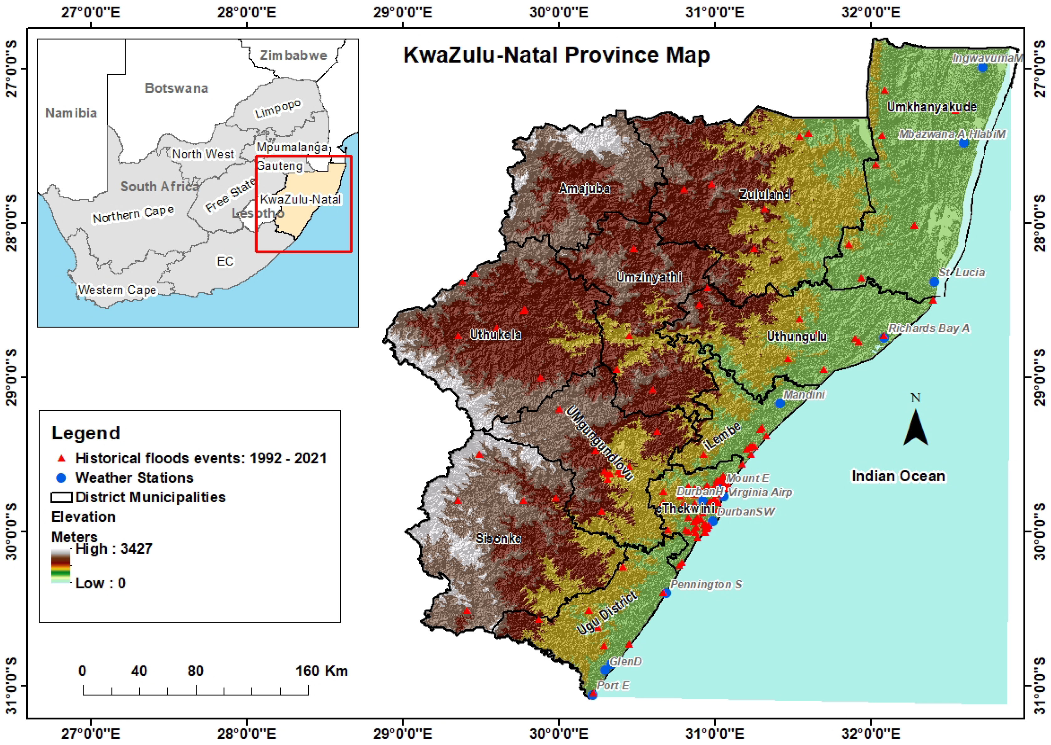
2.1. Study Area

Whilst this study focuses on the east coast (i.e., two corner coordinates: 28°52′58.133″ E, 28°41′7.93″ S and 32°52′6.283″ E, 26°51′54.895″ S) of South Africa, it extends (94,361 km2) well onto the interior plateau (Figure 1) which is the eastern province of KwaZulu-Natal. The western extent inland also allows us to track the development and propagation of the COL pressure systems, and their impacts. The study area includes complex topographic gradients from an interior plateau and to the Great Drakensberg escarpment and a narrow coastal area. The elevation of the study area ranges from 0 to 3442 m above sea level. Thus, the KwaZulu-Natal Province has a varied climate partly due to the complex topography, with a coastal region classified as subtropical climate (cfc), whereas the inland exhibits a temperate climate that is progressively cold due to the high altitude. It is characterised by minimum and maximum temperatures of 19.7 °C and 24.8 °C, respectively. In the last three decades (1992–2022), the coastal regions received an annual average rainfall of approximately 893 m–1009 mm, and whilst considered a summer rainfall region, significant amounts did fall during the dry season.
The warm Agulhas Current flowing south near the coast also partly accounts for the high rainfall experienced on the east coast. KwaZulu-Natal is home to over 11.1 million people and is ranked the second-most populous province in South Africa, after Gauteng. This area has been ravaged by floods (Figure 1 historical flood events), which have led to the destruction of critical infrastructure and loss of lives and livelihoods. In this area, one of the deadliest floods occurred between 16–18 April 2022, whereby 448 people lost their lives and thousands were displaced, causing a humanitarian crisis. The most affected municipality was eThekwini, which includes Durban city, the busiest shipping port in sub-Saharan Africa. Thus, floods threaten this coastal city transport infrastructure, causing trade delays and loss of revenue. Therefore, this warrants a study that focuses on the evolution and the impacts of the most recent flooding events along the KwaZulu Natal coastal region and to further predict the level of risk for a potential flooding in the entire province.

2.2. Rainfall, Temperature, and Circulation

Daily rainfall and maximum temperature observations were obtained from the South African Weather Service (SAWS) station network for the period 6–21 April 2022. The SAWS has an extensive network of automatic weather stations along the coast and the adjacent interior. Circulation variables including mean sea level pressure (MSLP), winds, geopotential height, and vertical velocity (ω) were obtained from the European Center for Medium-Range Weather Forecasts (ECMWF) ERA5 reanalyses [36]. The ERA5 reanalyses are obtained at a resolution of 31 km which is adequate for analysis of COL weather systems which are synoptic scale features. Thus, we plotted daily surface and upper air circulation variables across a domain extending from 20–40° S and 10–50° E to capture the large-scale features of the circulation and how they propagated across eastern South Africa from 6–21 April 2022. As COLs are slow-moving weather systems, the daily time scale used in this study is appropriate to understand the evolution and propagation of these systems. Temperature and precipitation data from the ERA5 reanalyses were also analyzed and juxtaposed with the circulation. Infrared satellite images (10 microns) from the European Organization for the Exploitation of Meteorological Satellites (EUMETSAT) were also analyzed to show the extent of deep convection associated with the two COLs and their propagation.

2.3. Flood Risk Mapping

In this study, flood risk is conceptualised as a likelihood of an area to be affected by floods due to its environmental characteristics. Consequently, a total of 214 historical geographical positioning system (GPS) points of historically (1992–2022) flooded areas (Figure 1) and 11 environmental factors obtained and derived from different free and open sources (Table 1) were used to develop a flood risk map of Kwa-Zulu Natal Province, South Africa, using the MaxEnt model. The number of flooded points were considered adequate as the MaxEnt modelling technique has been proven to perform well with a minimum of 10 sampling points [37]. Since the MaxEnt model requires presence-only data, this current study focused only on areas where flood events were recorded from 1990 to 2022 in Caelum. The flooded areas were randomly distributed across the study area and the data were split into 75% for model training and 25% for model testing. Environmental variables (Table 1) used in this study were selected based on preconceived knowledge and their relevance in the determination of flood risks as well as their wide-ranging applications in flood hazard mapping, as demonstrated in previous studies [38,39,40,41,42]. Prior to data assimilation into MaxEnt model, all the environmental factors were reprojected to World Geodetic System 84, Universal Transverse Mercator Zone 35 South (WGS_ 1984_UTM_Zone_35S) and resampled to 90 m × 90 m spatial resolution to ensure the same number of grid columns and rows. In a case where some data were in a vector format (e.g., distance to rivers), it was then rasterized and converted to a MaxEnt supported ACII file using the ArcGIS 10.6 (ESRI, Redlands, CA, USA) software.
Maximum entropy (MaxEnt) (https://biodiversityinformatics.amnh.org/open_source/maxent/(accessed on 14 September 2022)) was utilized to model and predict areas that are likely to experience flooding in the coastal province of Kwa-Zulu Natal. MaxEnt is a machine learning approach normally used for modeling species niches and distributions [43]. However, this model has recently proven to be very effective for predicting and mapping flood risk areas [44,45]. This model is composed of two main components, namely entropy and constraints. Entropy focuses on the model calibration to find the distribution that is most spread out, or closest to uniform throughout the study region, whereas constraints involve the rules that constrain the predicted distribution. These rules are based on the values of the environmental variables of the locations where species (in this case, floods) have been observed [43]. In addition, the Jackknife test was used to analyse the contribution rate and importance of each variable while Area Under Curve (AUC) Receiver Operating Characteristic (ROC) was used to judge the accuracy of the MaxEnt model in predicting flood risks in the study area. In general, an AUC of 0.5 suggests that the model performance is poor (i.e., not recommended for mapping floods), 0.7 to 0.8 is considered acceptable, 0.8 to 0.9 is considered excellent, and more than 0.9 is considered outstanding [46]. The flood risk map was finally derived from the logistic output of MaxEnt. The flood risk index obtained from MaxEnt ranged from the lowest “0” to the highest “1”. It was then classified into five flood risk classes (i.e., very low risk; low risk; moderate risk; high risk; and very high risk), using natural breaks [41] in ArcGIS 10.6 (ESRI, USA).

3. Results and Discussion

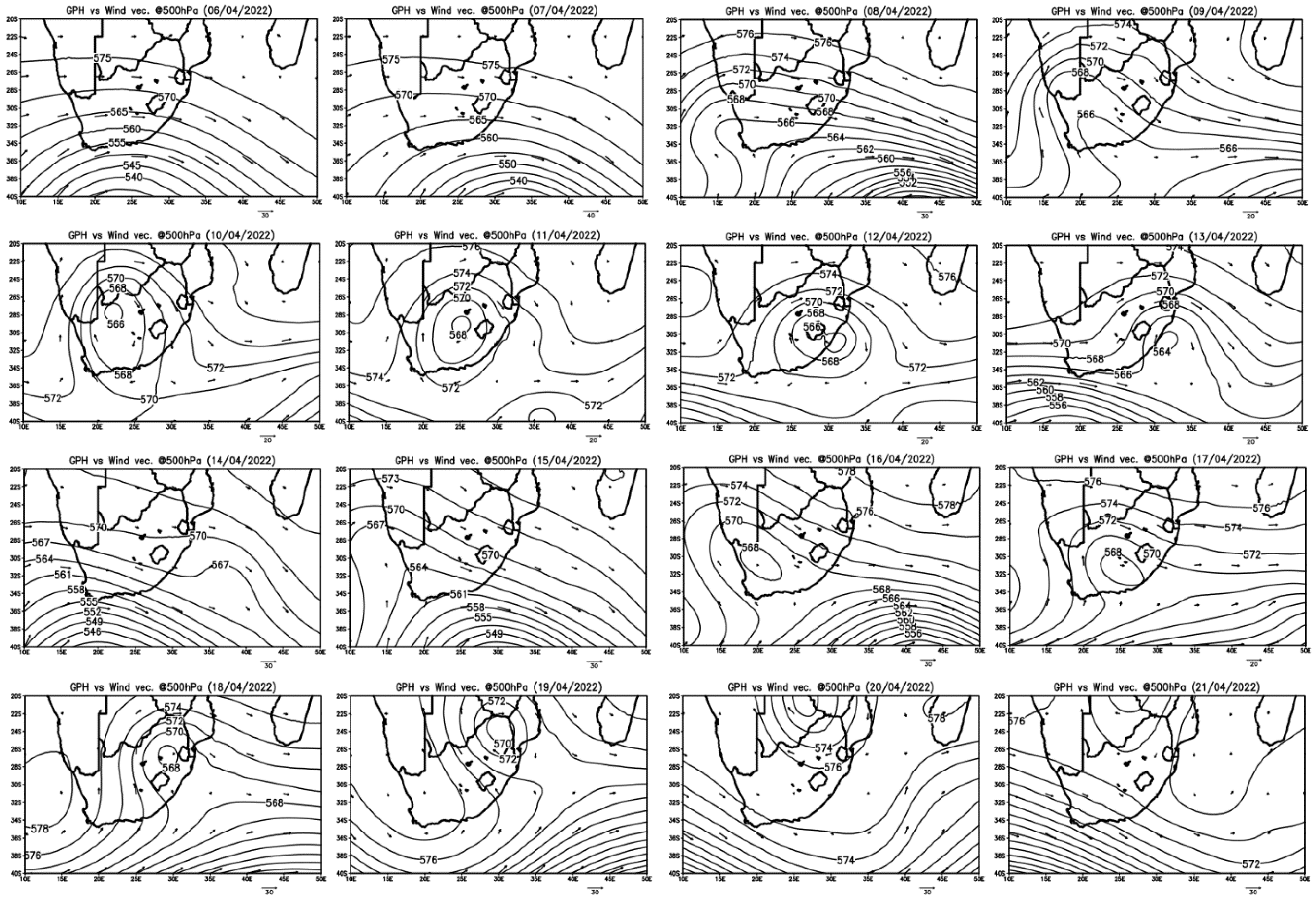
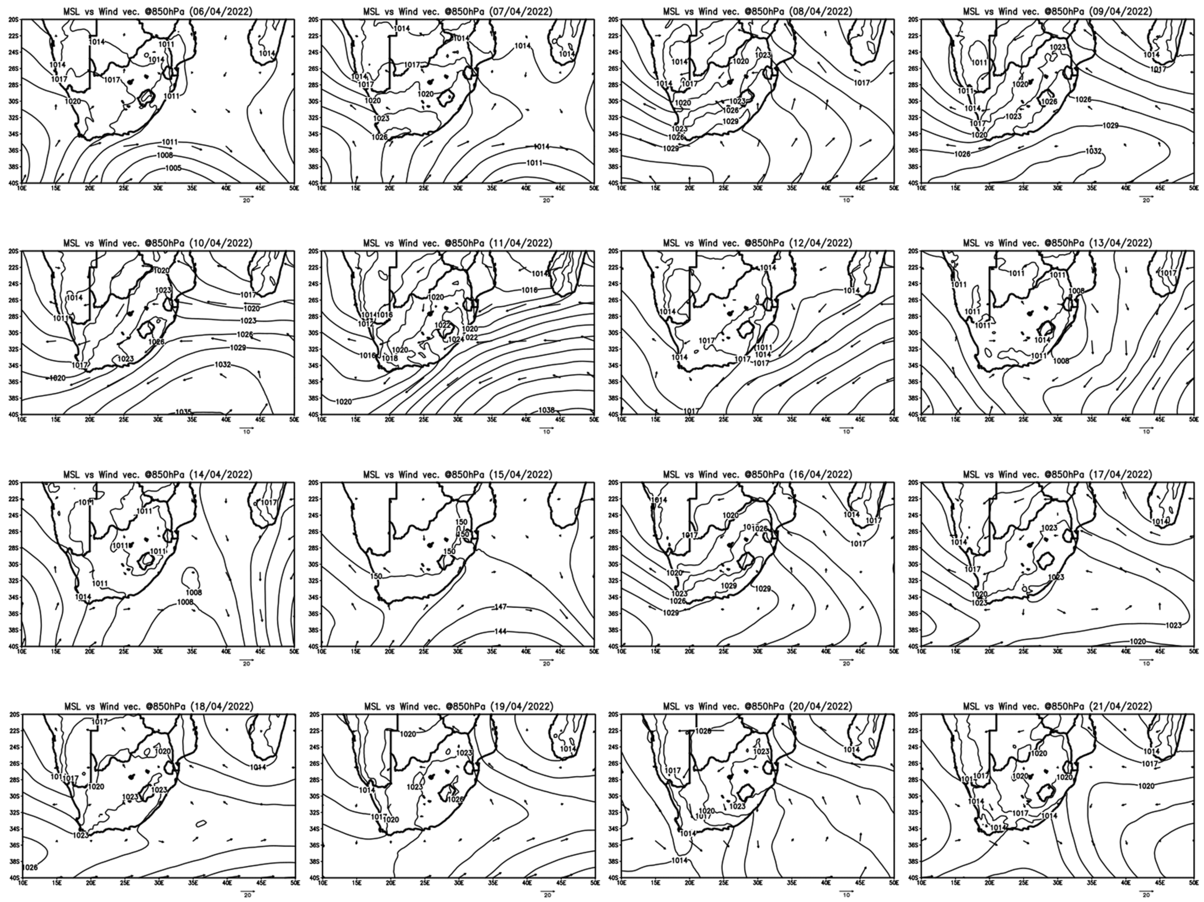
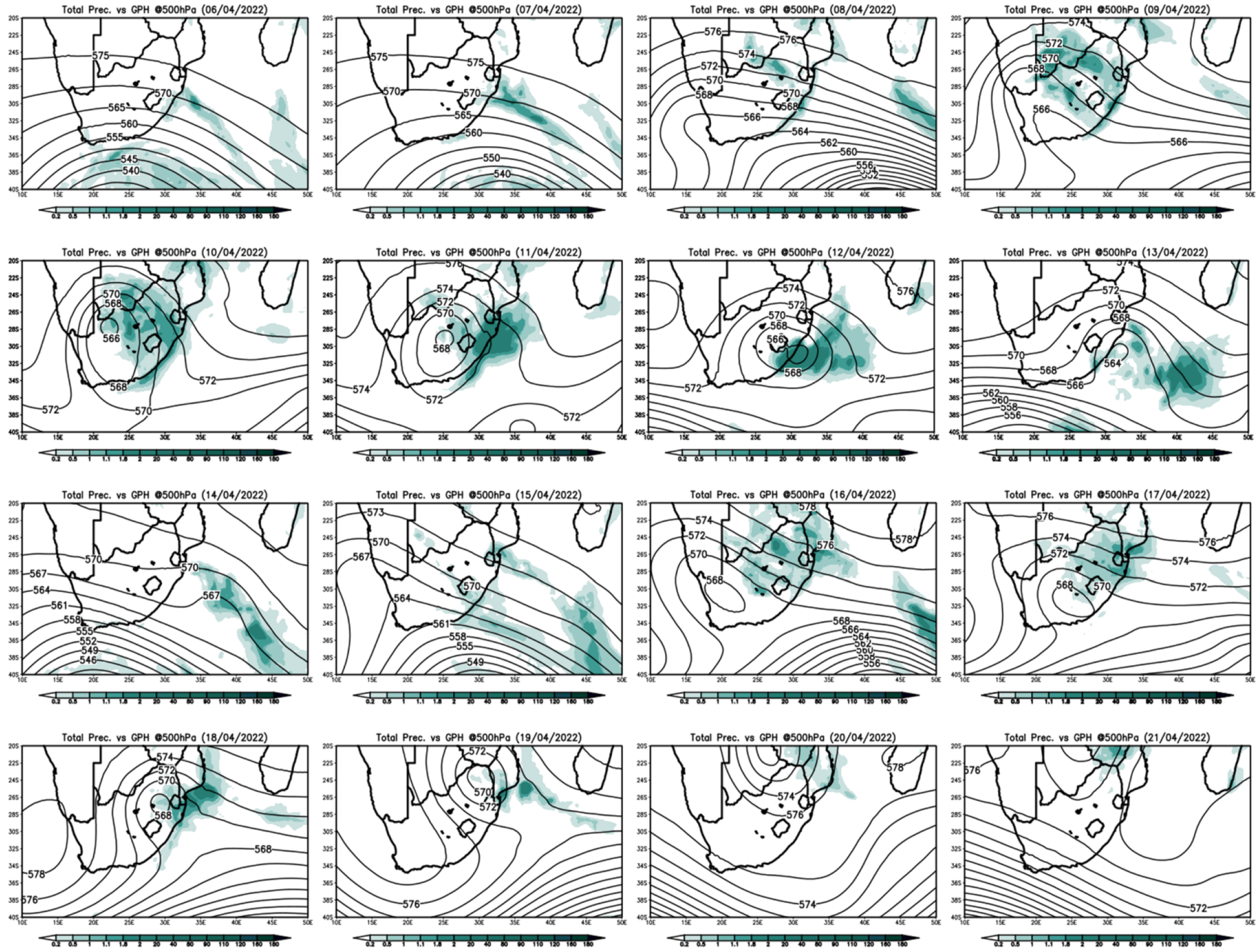
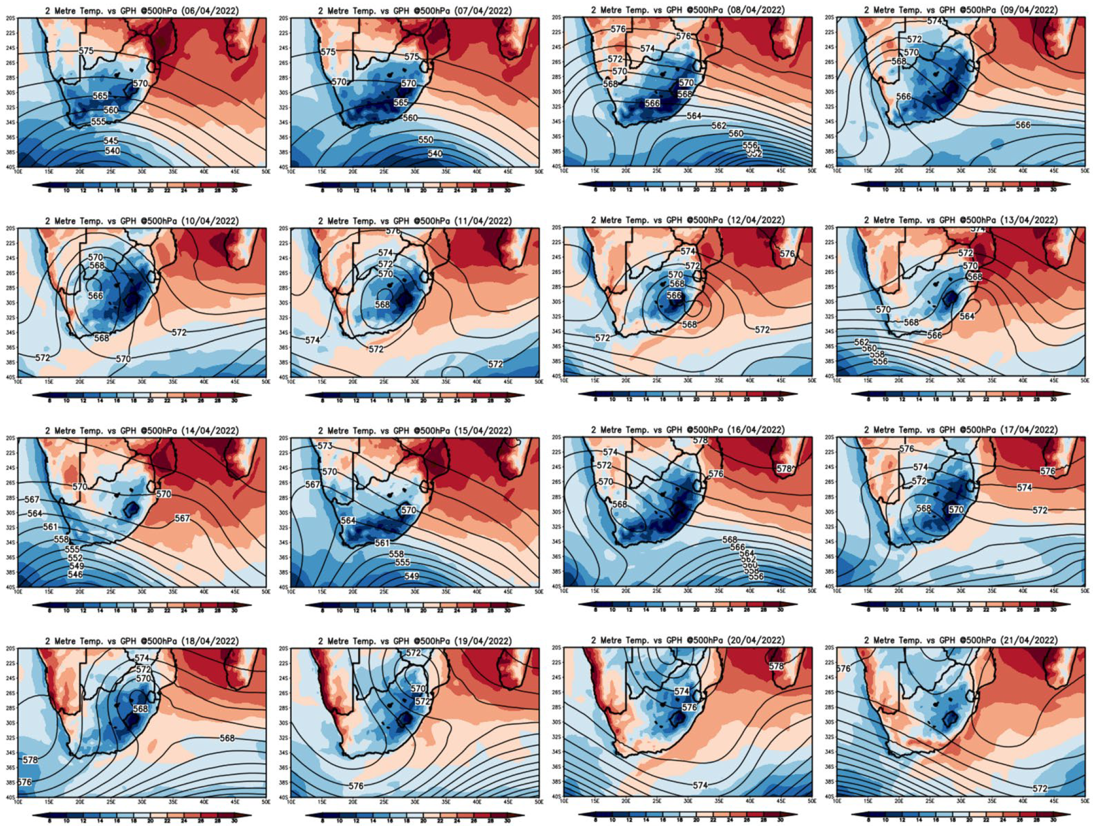
3.1. Meteorological Structure of Extreme Rainfall and Floods

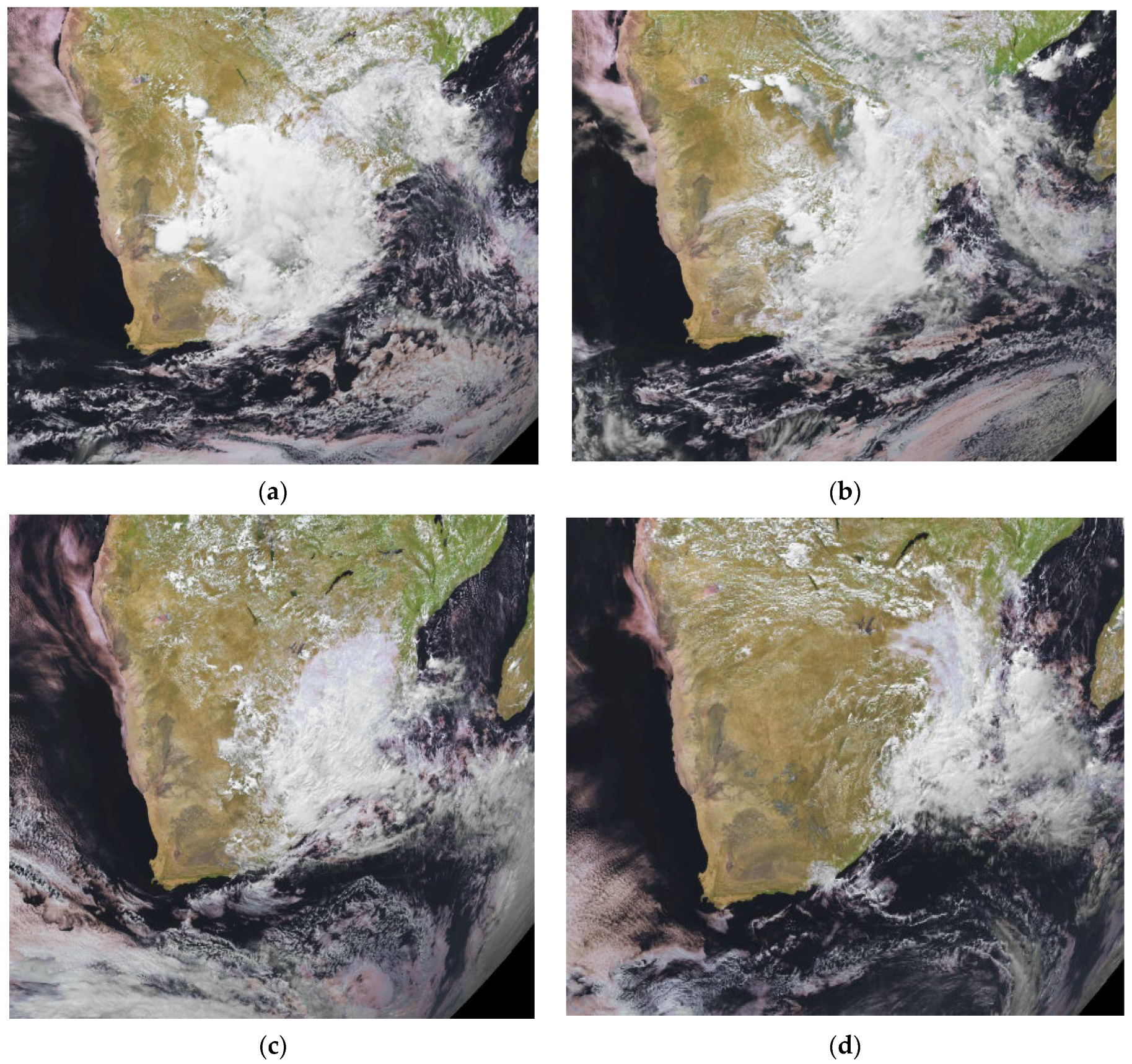
3.1.1. Accumulated Observed Rainfall along the East Coast

Extreme rainfall fell over eastern South Africa at the end of the 2021/2022 summer rainfall season. These floods occurred in the middle of a prolonged La Nina episode that began in 2020. La Nina events tend to be associated with higher-than-normal rainfall over South(ern) Africa [47] and flood events are more common under this phase than during the El Nino counterpart. During 6–21 April 2022, several rainfall stations across eastern KwaZulu-Natal Province recorded cumulative rainfall amounts exceeding 200 mm in 16 days. The highest accumulated falls (>400 mm) are shown in Table 2, and we found that they were all from the SAWS stations along the coastal area (Figure 1). This is a most significant finding which warrants further investigation. The heaviest falls of rain during the period were at Ingwavuma Manguzi (857.7 mm) on the north coast and Margate Airport (725.5 mm) on the south coast (Table 2). Other notable amounts shown in Table 2 include Margate (593 mm), Mandini (593 mm), Glen Doone (587 mm), and St Lucia Forest (583 mm). The rainfall amounts decreased considerably inland, with increasing distance from the coast.
From this rainfall distribution, the following key questions arise:
  • Why were extreme rainfall amounts (>400 mm) restricted to the coastal area without extending farther inland?
  • Whilst we have shown that the entire coastal area was affected by extreme rainfall, why was the extensive damage to infrastructure and loss of lives mainly focused on the eThekwini District?
The questions above suggest that there may be other non-meteorological factors which contribute significantly to flooding, flood risk, and flood-related natural disasters over the KwaZulu-Natal Province.
Previous COLs have also caused extreme rainfall along the east coast, with more than 900 mm during September 1987 [17]). The resulting flood was described as a 120–150-year flood event [24], leaving 506 people dead, more than 50,000 homeless, and at least 14 bridges destroyed [48]. Whether these big COL events will become more frequent or not along the east coast in the future is a critical research question which has implications for disaster management in KwaZulu-Natal.

3.1.2. Evolution of the COL Pressure Systems

Using geopotential heights at 500 hPa, a series of two cut-off low systems were identified over the South African domain between the 6th and 21st of April 2022 (Figure 2). An upper air trough was identified on the 6th of April 2022, deepening on the 8th and 9th of April. A fully developed COL system could be identified on the 10th, with the core over the western parts of the country. On the 11th, the system was located over the central parts of the country, gradually propagating to lie over the southeastern parts of the country on the 12th of April. The first system reached the dissipating stage on the 13th and 14th of April 2022, moving off into the Indian Ocean. Eventually, on the 15th of April, a new upper trough was identified over the western parts of the country. This system became fully developed on the 16th of April and propagated across the central and northeastern parts of the country between the 17th and 20th of April. Comparing the two, the first event was slightly deeper with geopotential heights below 566 decameters and its core at 500 hPa (Figure 2), whilst the second system (568 decameters) was slightly displaced to the northeast. The EUMETSAT satellite images also show the differences in spatial extent and location of the two COLs (Figure 3). The first COL affected a large area of the central interior from the 9th to 10th of April, whilst the second system was slightly smaller and more orientated to the northeast, affecting the southern districts of Zimbabwe and Mozambique. Climatologically, COLs mostly affect the South African domain, and few have been observed to affect neighbouring northern countries of Namibia, Botswana, Zimbabwe, eSwatini, and Mozambique [17].
Most rainfall-producing COLs are associated with ridging anticyclones near the surface [7], which provide the low-level moisture and dynamical trigger upon interaction with the steep escarpment. Near the surface, a Type-S ridging anticyclone (Figure 4) affected the south coast and steered cool and moist air from the Southern Ocean. A Type-S ridging anticyclone is centered south of 40° S, remains south of the country, and tends to have isobars that are perpendicular to the east coast [49]. Type-N ridging anticyclones evolve quite differently, centered north of 40° S and with higher MSLP anomalies [49]. The Type-S ridging anticyclone evolved from the 6th to 10th of April, budding off onto the Indian Ocean anticyclone. A surface trough developed along the east coast on 11 April, developing into a subtropical low-pressure system which exhibited tropical characteristics overnight. This subtropical cyclone was subsequently named Issa by the Tropical Cyclone Center at La Reunion. A combination of a cold-cored COL in the mid troposphere with a warm-cored subtropical cyclone at the surface is a most unusual occurrence. The subtropical cyclone Issa resulted in enhanced flow (gale force winds) of low-level moist air across the Agulhas Current, interacting with the coastal escarpment and providing more lift and moisture for deep convection. Thus, the occurrence of Issa accounted for the extreme rainfall that accumulated along the coast during 11–12 April 2022. As the subtropical cyclone Issa gradually moved off into the Indian Ocean, a new Type-S ridging process began on the 14th. This ridge extended to the east coast from the 16th to 19th of April, co-locating with the upper COL.

3.1.3. Spreading of Daily Rainfall

During the developing (8–9 April) stage of the first system, some rainfall activities were observed over the central parts of the country due to the presence of the upper trough. Rainfall amounts between 20 and 80 mm were observed over the central and northern parts of the country as the system became fully developed on 10 April (Figure 5). High accumulation of rainfall was observed over the southeastern parts of the country in KwaZulu-Natal Province, exacerbated by the identified easterly gale force winds which led to high moisture advection from the South Indian Ocean. The dissipating stages (13–14 April) of the system were marked with rainfall activity over the ocean with little or no rainfall observed in the country. However, the recovery period was short lived as the second system started producing high rainfall that was distributed over the central and northeastern parts of the country during the matured stages (16th and 17th). High amounts of rainfall were further observed over the eastern parts of the country (including the coast) on 18 April. We found that more rainfall fell along the east coast during the first COL event, particularly 11–12 April 2022, whilst the second COL event produced rainfall mainly on the north coast of the province from 17–18 April. Thus, extreme daily rainfall events affected the east coast for only five days, apart from hampering the recovery efforts for flood ravaged communities.

3.1.4. Daily Temperature Distribution

Typically, COLs are cold-cored and associated not only with heavy persistent rainfall, but also with bitter cold weather conditions, and often with snow falls over high ground in South Africa. As expected, 2 m surface air temperatures during the study period showed colder conditions (<20 °C) across much of South Africa (Figure 6), with significantly warmer temperatures observed in the neighbouring countries. Cold conditions were observed across the country during the period of the two identified systems (Figure 6). The matured stages of the systems were marked with low temperature over most central parts of the country, whilst the dissipating stages were observed with increasing temperature. In the first COL case, very cold conditions occurred (8 April) in KwaZulu-Natal before the arrival of the COL core. By the time of the heavy rainfall and flood (11–12 April), temperatures were not as cold, as the ridging anticyclone had been replaced by the subtropical cyclone Issa with tropical characteristics. The second COL event produced very cold conditions mainly along the east coast and the Great Escarpment during heavy rainfall because of the presence of a ridging anticyclone advecting cold air from the Southern Ocean. Colder conditions were observed in the south and east coasts along the high ground along the Great escarpment. The very cold conditions that affected the flooded area would have worsened the plight of thousands of households whose houses and belongings had been destroyed by flood waters.

3.2. Flood Risk Mapping

3.2.1. Analysis of Variable Contributions to Flood Risks

Table 3 shows the results of the Jackknife test that was used to estimate the relative contribution of each environmental variable in predicting flood risks in the study area. The results show that the Normalised Difference Vegetation Index (NDVI) and Terrain Ruggedness Index (TRI) have no associated relationship with flood risk in this study; therefore, they were omitted, and the remaining nine variables were utilized to run the MaxEnt model. The results revealed that land cover (52.8%) contributed the most to the flood risk of Kwa-Zulu Natal, followed by elevation (16.8%) and lithology (15.5). The total contribution rate of the latter three factors was 85.4%, whereas slope, average annual rainfall, distance from the rivers, Stream Power Index (SPI), drainage density, and Topographic Wetness Index (TWI) contributed about a total of 15% to flood risk. This is similar to a previous study [50], which indicated that land cover contributed the most (40.8%) to the modelling of flood risk in the southern Bagmati corridor of Nepal. Land cover/use was found to be the most important variable for flood risk mapping since it is closely related to population needs, such as conversion of agricultural and forest land to urban areas, conversion of forest to farmland, and reduction of involuntary or unethical slope for infrastructure developments [51]. For instance, the study by [29] has demonstrated that land cover/use changes, such as rapid urban development coupled with increasing impermeable surfaces, poor drainage system, and changes in extreme precipitation, are the most important factors that lead to increased urban flooding. In contrast to our findings, [44] and [39] discovered that proximity to rivers carried more weight in determining flood risk in Iran, whilst [45] revealed that rainfall was the most influential environmental variable in the Philippines.
In addition, the response curves for each variable are studied and their individual relationship with flood risk is summarised in Table 1. The findings show that elevation, slope, and SPI have an inverse relationship with flood risk. However, it also depends on slope length, since the longer the slope length, the greater the volume of water, flow speed, and inertia force, which increase flood risk [52]. This ascertains that flood hazards more often occur in areas that have low topographic elevations than those characterised by higher altitudes. It is also important to note that the KwaZulu-Natal region has a complex relief system that consists of the Great Escarpment and coastal plain. The land rises steeply from the coastal plain to plateau. This affects the human population distribution as well; hence, many communities are concentrated on the gentle slopes and lower elevation coastal plains where flooding frequency has increased lately, especially in towns, such as Durban. These results concur with those of [50,53], where the authors have also found that a basin with a gentle slope has a relatively higher number of floods than a basin with a steep slope. Conversely, average rainfall, TWI, and drainage density are shown to have a direct relationship with flood risk index in this study. The latter aligns with [30], who has also demonstrated that an increase in rainfall, coupled with other factors, such as elevation, land cover type, and slope, leads to floods. On the other hand, TWI has also been documented as a more cost-efficient approach to flood determination than conventional hydrodynamic models [54]. The results of this study also concur with those of [55], which has indicated that higher drainage densities result in increased runoff flow which is associated with high flood risk.

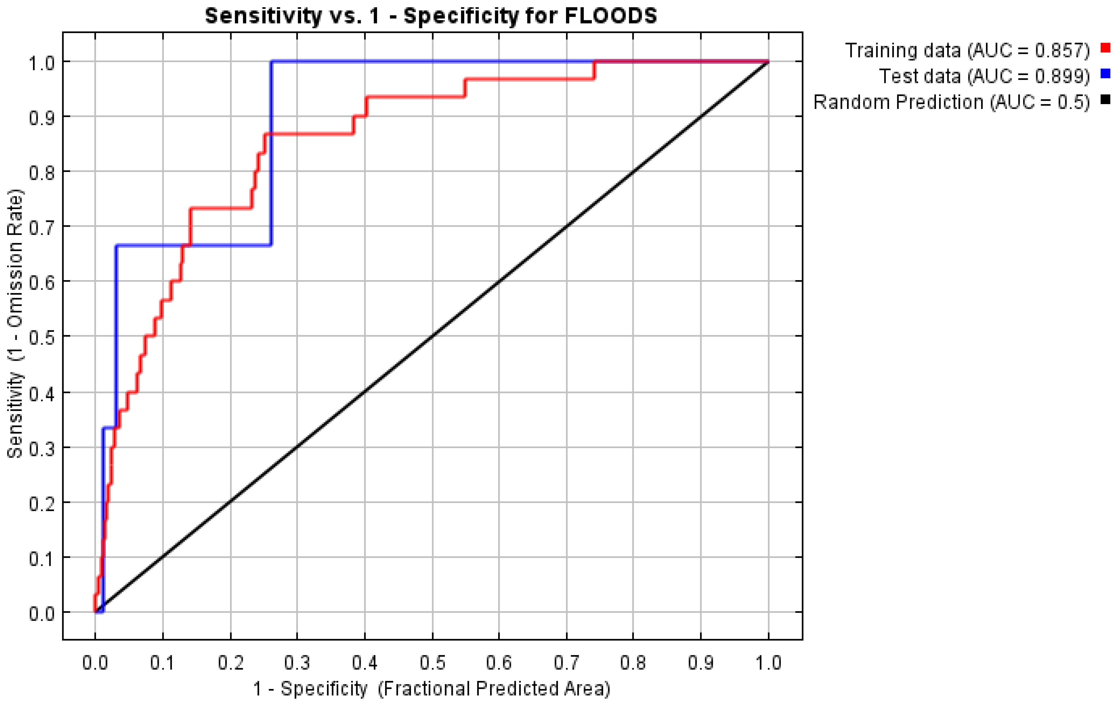
3.2.2. MaxEnt Model Performance in Mapping Flood Risks

Figure 7 depicts the AUC-ROC of the MaxEnt model’s performance. This curve contains the red line that shows the mean value for the MaxEnt model and the blue line that indicates the ±1 standard deviation. The results show that the AUC is 0.899 with a standard deviation of 0.065 (Figure 7). The AUC is close to 0.9 or higher than 0.8 and, as such, the MaxEnt model has indicated a good estimation of the spatial distribution of risks to flooding at a provincial scale based on environmental factors. This model’s performance, however, is lower than that of [44] at 97.2% and [39] at 90%, but slightly higher than [38] at 88.5% and [42] at 76%. Nonetheless, the model is informative and could be used for subsequent flood risk mapping since an AUC of 80% to 90% is considered excellent [46].

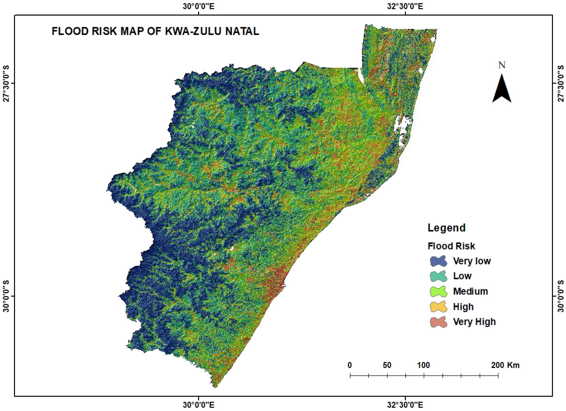
3.2.3. Flood Risk Map

The flood risk analysis (Table 4) shows that about 5563.56 km2 (6.42%), 10,191.24 km2 (11.76%), 18,766.59 km2 (21.66%), 27,572.76 km2 (31.82%), and 24,548.28 km2 (28.33%) of the total area of Kwa-Zulu Natal is at a very high risk, high risk, moderate risk, low risk, and very low risk, respectively. Areas at the very high and high risk account for about 17.5% of Kwa-Zulu Natal, whereas those that are identified as having low and very low risk account for 60.15% of the total area. The most dominant class is medium-risk areas which account for 31.82% of the total area. The flood risk map (Figure 8) reveals that high risk is mainly distributed along the southwest coast of Kwa-Zulu Natal, and it includes areas such as Durban, Mtunzini, Scottburgh, Port Shepstone, and Mtwalume. The high-risk areas also extend into the interior towards but not limited to Pietermaritzburg, Vryheid, Nongoma, and eMondlo. This higher level of risk could be attributed to an interplay of low elevation, high built-up area, slope, lithology, and other factors. The flood risk map results concur with the 8–9 April 2022 flood events in KwaZulu Natal, which killed people and destroyed infrastructure in the latter mentioned areas. This then demonstrates the robustness of the MaxEnt machine learning approach in flood risk prediction.

4. Conclusions and Recommendations

During April 2022, extreme rainfall led to floods along the east coast of South Africa, causing more than 448 deaths, destruction of infrastructure, and loss of livelihoods. Extensive flooding was caused by two consecutive COLs that affected the country less than a week apart, with the second system compounding an already dire situation. Extreme rainfall amounts exceeding 500 mm affected mostly the coastal area. We can also conclude that the April 2022 floods were not the first in KwaZulu-Natal caused by a COL, and we speculate they may not be the last. This realisation underscores the need for urgent interventions to avoid future loss of lives and livelihoods and damage to infrastructure, as recorded in past events.
It is very rare that two COLs occur successively and affect the same region barely five days apart over the South African domain. We found that the first COL was much larger and deeper, and was associated with more rainfall along the east coast than the second COL. In addition, the two COLs were both initially associated with Type-S ridging anticyclones near the surface. However, the first and more destructive COL interacted with the subtropical cyclone Issa, resulting in extreme rainfall along the coastal area. The low-level gale force winds were advected onshore by Issa across the warm Agulhas Current and interacted with the coastal escarpment to enhance lifting and deep convection. The occurrence of Issa and its tropical characteristics is unprecedented and requires rigorous investigation. A high-resolution model simulation of the event is necessary to understand the dynamics of the low-level, low-pressure system that developed off the east coast. We are also aware that some deep COLs have been found to extend to the surface, particularly during the austral autumn [56].
The second COL event affected the north coast more, whereas the initial COL affected the entire coastline. However, both systems produced heavy rainfall and affected the eastern half of the country, with an intervening period of only two days of no rain between the two COL weather systems. Whilst the entire KwaZulu-Natal coastline was affected by extreme and unseasonal rainfall amounts, the flooding, destruction of infrastructure, and loss of lives were mainly focused on a district around the Durban metropolitan city (eThekwini) and its precincts. Our study has revealed that this area is at high flood risk of historical and future events. Some climate change projections suggest increasing frequency of extreme rainfall events over eastern South Africa under low mitigation scenarios. In addition, this study has revealed that land use/cover as well as elevation are the most important flood conditioning factors. Therefore, with rapid increase in urbanisation due to the rise in population, more people are most likely to occupy low lying areas, remove natural vegetation, flatten steep slopes for construction, and install paving on the ground, thus exacerbating flood risks. Furthermore, Kwa-Zulu Natal is a highly densely populated area with about 122 people per km2 and the majority people are concentrated in cities, including Durban and Pietermaritzburg, which, according to our MaxEnt model, have been classified as high-risk areas. Although most of the Kwa-Zulu Natal province has been classified to have a moderate, low, or very low risk, the dangers are still eminent due to frequent extreme weather events. Therefore, extreme caution should always be exercised, especially since the province is characterised by steep slopes when moving from the coastal plains to the Great Escarpment and the plateau, which can be associated with landslides in the events of high rainfall and floods. The AUC- ROC diagram was employed to estimate the accuracy of our flood risk map; the results reveal the robustness of the MaxEnt model in producing flood risk maps, and the model has managed to yield an acceptable accuracy of almost 90% (AUC = 0.899). This implies that the maps can be reliable for making decisions concerning floods. The generated results of the flood risk map could help local government, civil protection, and disaster management authorities identify and plan to mitigate future flood risk and minimise loss of lives.
The key recommendations for disaster risk reduction include a review of drainage systems in the settlements affected by (or at risk of) floods and conducting comprehensive flood vulnerability assessments. Vulnerability assessments should consider not only physical, but also social and economic factors. Several other regions around the world experience flooding perennially, such as those that experience Monsoon rains in India and Bangladesh. With increasing flood risk in coastal areas globally, mangroves have been found to help absorb large amounts of water and mitigate against flooding with benefits to people in Vietnam, India, and Bangladesh [57]. In a study of some of the worst natural disasters [58], it is determined that disasters do not occur due to a lack of forecasts and early warning systems, but rather due to inadequate communication and response capability. Dissemination of weather warnings can also be extended to include community radio stations, vehicles, and traditional leadership, including the use of local police enforcement [59]. While governments have a responsibility to establish functional multi-hazard early warning systems [60], communities and local leaders in Puerto Rico have learnt to organise themselves and help each other during and after flood events [61]. The lessons learnt by these territories to live with floods and protect lives can also be adopted to South Africa’s KwaZulu-Natal Province. Our study contributes to natural disaster risk reduction on the east coast of South Africa, amidst a changing climate characterised by increased intensity of storms.

Author Contributions

F.M.M. and H.C. conceptualized the study; T.P.M., I.L.M., W.M., M.C.M. and F.M.M. performed data analysis and ran the model; R.B.M., M.C.M., T.P.M. and H.C. wrote the initial draft; J.M.L., T.P.M. and H.C. revised and edited the manuscript. All authors have read and agreed to the published version of the manuscript.

Funding

This research received no external funding.

Data Availability Statement

The data analysed in this study is available publicly on the archives of the European Center for Medium Range Weather Forecasts (ECMWF), European Organisation for the Exploitation of Meteorological Satellites (EUMETSAT), United States Geological Survey and upon request from the South African Weather Service (SAWS) and Agricultural Research Council (ARC).

Acknowledgments

The authors acknowledge the South African Weather Service for the daily rainfall and temperature observations and the National Disaster Management Center for impact data via the Caelum database. The satellite images were obtained from EUMETSAT whilst the climate reanalyses analysed here were obtained from the European Center for Medium-Range Weather Forecasts (ECMWF).

Conflicts of Interest

The authors declare no conflict of interest.

References

  1. Hoegh-Guldberg, O.; Jacob, D.; Bindi, M.; Brown, S.; Camilloni, I.; Diedhiou, A.; Djalante, R.; Ebi, K.; Engelbrecht, F.; Guiot, J.; et al. Impacts of 1.5 °C Global Warming on Natural and Human Systems; Global Warming of 1.5 °C; IPCC Secretariat: Geneva, Switzerland, 2018. [Google Scholar]
  2. Gijben, M.; de Coning, C. Using Satellite and Lightning Data to Track Rapidly Developing Thunderstorms in Data Sparse regions. Atmospher 2017, 8, 67. [Google Scholar] [CrossRef] [Green Version]
  3. Mbokodo, I.; Bopape, M.-J.; Chikoore, H.; Engelbrecht, F.; Nethengwe, N. Heatwaves in the Future Warmer Climate of South Africa. Atmosphere 2020, 11, 712. [Google Scholar] [CrossRef]
  4. Scholes, R.; Engelbrecht, F. Climate Impacts in Southern Africa during the 21st Century; Report for Earthjustice and the Centre for Environmental Rights; Global Change Institute, University of the Witwatersrand: Johannesburg, South Africa, 2021. [Google Scholar]
  5. Ziervogel, G.; New, M.; Archer van Garderen, E.; Midgley, G.; Taylor, A.; Hamann, R.; Stuart-Hill, S.; Myers, J.; Warburton, M. Climate change impacts and adaptation in South Africa. Wiley Interdiscip. Rev. Clim. Change 2014, 5, 605–620. [Google Scholar] [CrossRef]
  6. Stats SA. How Unequal Is South Africa. Available online: https://www.statssa.gov.za/?p=12930 (accessed on 14 August 2022).
  7. Muofhe, T.P.; Chikoore, H.; Bopape, M.M.; Nethengwe, N.S.; Ndarana, T.; Rambuwani, G.T. Forecasting intense cut-off lows in South Africa using the 4.4 km Unified Model. Climate 2020, 8, 129. [Google Scholar] [CrossRef]
  8. Chikoore, H.; Bopape, M.M.; Ndarana, T.; Muofhe, T.P.; Gijben, M.; Munyai, R.B.; Manyanya, T.C.; Maisha, R. Synoptic structure of a sub-daily extreme precipitation and flood event in Thohoyandou, northeastern South Africa. Weather. Clim. Extrem. 2021, 33, 10327. [Google Scholar] [CrossRef]
  9. Hart, N.C.; Reason, C.J.; Fauchereau, N. Building a tropical–extratropical cloud band metbot. Mon. Weather. Rev. 2012, 140, 4005–4016. [Google Scholar] [CrossRef]
  10. Blamey, R.C.; Reason, C.J.C. Mesoscale convective complexes over southern Africa. J. Clim. 2012, 25, 753–766. [Google Scholar] [CrossRef] [Green Version]
  11. Webster, E.M. A Synoptic Climatology of Continental Tropical Low Pressure Systems over Southern Africa and Their Contribution to Rainfall over South Africa. MSc Dissertation, University of Pretoria, Pretoria, South Africa, 2019. [Google Scholar]
  12. Jury, M.R. Climate trends across South Africa since 1980. Water SA 2018, 44, 297–307. [Google Scholar] [CrossRef] [Green Version]
  13. MacKellar, N.; New, M.; Jack, C. Observed and modelled trends in rainfall and temperature for South Africa: 1960–2010. S. Afr. J. Sci. 2014, 110, 7–8. [Google Scholar] [CrossRef] [Green Version]
  14. Kruger, A.C. Observed trends in daily precipitation indices in South Africa: 1910–2004. Int. J. Climatol. A J. R. Meteorol. Soc. 2006, 26, 2275–2285. [Google Scholar] [CrossRef]
  15. Roy, S.S.; Rouault, M. Spatial patterns of seasonal scale trends in extreme hourly precipitation in South Africa. Appl. Geogr. 2013, 39, 151–157. [Google Scholar]
  16. Kruger, A.C.; Nxumalo, M.P. Historical rainfall trends in South Africa: 1921–2015. Water SA 2017, 43, 285–297. [Google Scholar] [CrossRef] [Green Version]
  17. Singleton, A.T.; Reason, C.J.C. Variability in the characteristics of cut-off low pressure systems over subtropical southern Africa. Int. J. Climatol. 2007, 27, 295–310. [Google Scholar] [CrossRef]
  18. Ndarana, T.; Rammopo, T.S.; Chikoore, H.; Barnes, M.A.; Bopape, M.M. A quasi-geostrophic diagnosis of the zonal flow associated with cut-off lows over South Africa and surrounding oceans. Clim. Dyn. 2020, 55, 2631–2644. [Google Scholar] [CrossRef]
  19. Favre, A.; Hewitson, B.; Lennard, C.; Cerezo-Mota, R.; Tadross, M. Cut-off lows in the South Africa region and their contribution to precipitation. Clim. Dyn. 2013, 41, 2331–2351. [Google Scholar] [CrossRef]
  20. Taljaard, J.J. Cut-off lows in the South African region. South African Weather Bureau Technical Paper 14; South African Weather Service: Pretoria, South Africa, 1985; p. 153. [Google Scholar]
  21. Singleton, A.T. Cut-Off Low Pressure Systems and Extreme Rainfall over South Africa. Ph.D. Thesis, University of Cape Town, Cape Town, South Africa, 2005. [Google Scholar]
  22. Molekwa, S. Cut-Off Lows over South Africa and Their Contribution to the Total Rainfall of the Eastern Cape Province. MSc Dissertation, University of Pretoria, Pretoria, South Africa, 2013. [Google Scholar]
  23. Platford, G.G. Protection against flood damage. In Proceedings of the South Africa Sugar Technologists’ Association; SASTA: Mount Edgecombe, South Africa, 1988. [Google Scholar]
  24. Badenhorst, P.; Cooper, J.A.G.; Crowther, J.; Gonsalves, J.; Laubscher, W.I.; Grobler, N.A.; Mason, T.R.; Illenberger, W.K.; Perry, J.E.; Reddering, J.S.V.; et al. Survey of September 1987 Natal Floods; South African National Scientific Programmes Report 164; CSIR: Pretoria, South Africa, 1989; p. 136. [Google Scholar]
  25. Caelum. Notable weather and weather-related events in geo-coded format: 1647–2021. South African Weather Service. 2021. Available online: https://www.weathersa.co.za/Documents/AnnualReports/SA_Weather_Services_Annual_Report_2020_21_Digital_Version_14092021122723.pdf (accessed on 15 August 2022).
  26. Seneviratne, X.; Zhang, M.; Adnan, W.; Badi, C.; Dereczynski, A.; Di Luca, S.; Ghosh, I.; Iskandar, J.; Kossin, S.; Lewis, F.; et al. Weather and Climate Extreme Events in a Changing Climate. In Climate Change 2021: The Physical Science Basis; Contribution of Working Group I to the Sixth Assessment Report of the Intergovernmental Panel on Climate Change; Masson-Delmotte, V., Zhai, P., Pirani, A., Connors, S.L., P’ean, C., Berger, S., Caud, N., Chen, Y., Goldfarb, L., Gomis, M.I., et al., Eds.; Cambridge University Press: Cambridge, UK, 2021. [Google Scholar]
  27. Kienberger, S. Spatial modelling of social and economic vulnerability to floods at the district level in Búzi, Mozambique. Nat. Hazards 2012, 64, 2001–2019. [Google Scholar] [CrossRef]
  28. Brunner, M.I.; Slater, L.; Tallaksen, L.M.; Clark, M. Challenges in modeling and predicting floods and droughts: A review. Wiley Interdiscip. Rev. Water 2021, 8, e1520. [Google Scholar] [CrossRef]
  29. Norallahi, M.; Seyed Kaboli, H. Urban flood hazard mapping using machine learning models: GARP, RF, MaxEnt and NB. Nat. Hazards 2021, 106, 119–137. [Google Scholar] [CrossRef]
  30. Jehanzaib, M.; Ajmal, M.; Achite, M.; Kim, T.W. Comprehensive Review: Advancements in Rainfall-Runoff Modelling for Flood Mitigation. Climate 2022, 10, 147. [Google Scholar] [CrossRef]
  31. Mgadle, A.; Dube, K.; Lekaota, L. Conservation and sustainability of coastal city tourism in the advent of Seal Level Rise in Durban, SouthAfrica. Tour. Mar. Environ. 2022, 17, 1–2. [Google Scholar]
  32. Busayo, E.T.; Kalumba, A.M. Recommendations for linking climate change adaptation and disaster risk reduction in urban coastal zones: Lessons from East London, South Africa. Ocean. Coast. Manag. 2021, 203, 105454. [Google Scholar] [CrossRef]
  33. Mather, A.A.; Stretch, D.D. A perspective on sea level rise and coastal storm surge from Southern and Eastern Africa: A case study near Durban, South Africa. Water 2012, 4, 237–259. [Google Scholar] [CrossRef]
  34. Dube, K.; Nhamo, G.; Chikodzi, D. Flooding trends and their impacts on coastal communities of Western Cape Province, South Africa. GeoJournal 2022, 87, 453–468. [Google Scholar] [CrossRef]
  35. Udo, F.; Naidu, M. Examining the Interplay between Economic Development and Local Women Vulnerability to Flood Impacts in Selected Local Areas in Durban, South Africa. J. Asian Afr. Stud. 2022, 00219096211069646. [Google Scholar] [CrossRef]
  36. Hersbach, H.; Bell, B.; Berrisford, P.; Hirahara, S.; Horányi, A.; Muñoz-Sabater, J.; Nicolas, J.; Peubey, C.; Radu, R.; Schepers, D.; et al. The ERA5 global reanalysis. Q. J. R. Meteorol. Soc. 2020, 146, 1999–2049. [Google Scholar] [CrossRef]
  37. Wisz, M.S.; Hijmans, R.J.; Li, J.; Peterson, A.T.; Graham, C.H.; Guisan, A.; NCEAS Predicting Species Distributions Working Group. Effects of sample size on the performance of species distribution models. Divers. Distrib. 2008, 14, 763–773. [Google Scholar] [CrossRef]
  38. Davoudi Moghaddam, D.; Haghizadeh, A. Detection of Susceptible Areas to Flooding and its Most Important Contributing Factors Using the Maximum Entropy Model in the Tashan Watershed, Khuzestan. Watershed Manag. Res. J. 2020, 33, 94–109. [Google Scholar]
  39. Moradi, E.; Rajabi, A.; Shabanlou, S.; Yosefvand, F. Identification of the Most Important Environmental Variables in Spatial Prediction of Flood Prone Areas using the Maximum Entropy Model in Parts of Golestan Province. Iran. J. Soil Water Res. 2021, 52, 899–915. [Google Scholar]
  40. Eini, M.; Kaboli, H.S.; Rashidian, M.; Hedayat, H. Hazard and vulnerability in urban flood risk mapping: Machine learning techniques and considering the role of urban districts. Int. J. Disaster Risk Reduct. 2020, 50, 101687. [Google Scholar] [CrossRef]
  41. Davoudi Moghaddam, D.; Pourghasemi, H.R.; Rahmati, O. Assessment of the contribution of geo-environmental factors to flood inundation in a semi-arid region of SW Iran: Comparison of different advanced modeling approaches. In Natural Hazards Gis-Based Spatial Modeling Using Data Mining Techniques; Springer: Cham, Switzerland, 2019; pp. 59–78. [Google Scholar]
  42. Darabi, H.; Haghighi, A.T.; Mohamadi, M.A.; Rashidpour, M.; Ziegler, A.D.; Hekmatzadeh, A.A.; Kløve, B. Urban flood risk mapping using data-driven geospatial techniques for a flood-prone case area in Iran. Hydrol. Res. 2020, 51, 127–142. [Google Scholar] [CrossRef] [Green Version]
  43. Phillips, S.J.; Dudík, M.; Schapire, R.E. A maximum entropy approach to species distribution modeling. In Proceedings of the Twenty-First International Conference on Machine Learning, Banff, AB, Canada, 4–8 July 2004; p. 83. [Google Scholar]
  44. Javidan, N.; Kavian, A.; Pourghasemi, H.R.; Conoscenti, C.; Jafarian, Z.; Rodrigo-Comino, J. Evaluation of multi-hazard map produced using MaxEnt machine learning technique. Sci. Rep. 2021, 11, 1–20. [Google Scholar]
  45. Cabrera, J.S.; Lee, H.S. Flood risk assessment for Davao Oriental in the Philippines using geographic information system-based multi-criteria analysis and the maximum entropy model. J. Flood Risk Manag. 2020, 13, e12607. [Google Scholar] [CrossRef] [Green Version]
  46. Mandrekar, J.N. Receiver operating characteristic curve in diagnostic test assessment. J. Thorac. Oncol. 2010, 5, 1315–1316. [Google Scholar] [CrossRef] [Green Version]
  47. Chikoore, H.; Jury, M.R. South African drought, deconstructed. Weather. Clim. Extrem. 2021, 33, 100334. [Google Scholar] [CrossRef]
  48. Eyewitness News. Death, and survival, haunt KZN flood-stricken shack dwellers. 2022. Available online: ewn.co.za (accessed on 11 October 2022).
  49. Ndarana, T.; Rammopo, T.S.; Reason, C.J.C.; Bopape, M.M.; Engelbrecht, F.A.; Chikoore, H. Two types of ridging South Atlantic Ocean anticyclones over South Africa and the associated dynamical processes. Atmos. Res. 2022, 265, 105897. [Google Scholar] [CrossRef]
  50. Shreevastav, B.B.; Tiwari, K.R.; Mandal, R.A.; Singh, B. “Flood risk modeling in southern Bagmati corridor, Nepal”(a study from Sarlahi and Rautahat, Nepal). Prog. Disaster Sci. 2022, 16, 100260. [Google Scholar] [CrossRef]
  51. Sengani, F.; Mashao, F.M.; Allopi, D. An integrated approach to develop a slope susceptibility map based on a GIS-based approach, soft computing technique and finite element formulation of the bound theorems. Transp. Geotech. 2022, 36, 100818. [Google Scholar] [CrossRef]
  52. Nguyen, B.D.; Minh, D.T.; Ahmad, A.; Nguyen, Q.L. The role of relative slope length in flood hazard mapping using AHP and GIS (case study: Lam River Basin, Vietnam). Geogr. Environ. Sustain. 2020, 13, 115–123. [Google Scholar] [CrossRef]
  53. Zeng, J.; Li, C.; Liu, J.; Li, Y.; Hu, Z.; He, M.; Zhang, H.; Yan, H. Ecological assessment of current and future Pogostemon cablin Benth. potential planting regions in China based on MaxEnt and ArcGIS models. J. Appl. Res. Med. Aromat. Plants 2021, 24, 100308. [Google Scholar]
  54. Pourali, S.H.; Arrowsmith, C.; Chrisman, N.; Matkan, A.A.; Mitchell, D. Topography wetness index application in flood-risk-based land use planning. Appl. Spat. Anal. Policy 2016, 9, 39–54. [Google Scholar] [CrossRef]
  55. Dang, M.T.; Nguyen, D.B. Application of GIS technology to establish a drainage density hierarchical map for flood hazard zoning in Lam river basin. J. Min. Earth Sci. 2018, 59, 32–42. [Google Scholar]
  56. Barnes, M.A.; Ndarana, T.; Landman, W.A. Cut-off lows in the Southern Hemisphere and their extension to the surface. Clim. Dyn. 2021, 56, 3709–3732. [Google Scholar] [CrossRef]
  57. Menendez, P.; Losada, I.J.; Torres-Ortega, S.; Narayan, S.; Beck, M.W. The Global Flood Protection benefits of mangroves. Sci. Rep. 2020, 10, 4404. [Google Scholar] [CrossRef] [Green Version]
  58. De Perez, E.C.; Berse, K.B.; Depante, L.A.C.; Easton-Calabria, E. Learning from the past in moving to the future: Invest in communication and response to weather early warnings to reduce death and damage. Clim. Risk Manag. 2022, 38, 100461. [Google Scholar] [CrossRef]
  59. Chikoore, H.; Unganai, L. Integrating climate forecast information in agricultural management: A perspective from southern Africa. In Proceedings of the Open Meeting of the Global environmental Change Research Community, Rio de Janeiro, Brazil, 6–8 October 2001. [Google Scholar]
  60. WMO. Multi-Hazard Early Warning System: A Checklist. 2022. Available online: https://public.wmo.int (accessed on 17 November 2022).
  61. The New Humanitarian. In Storm-Hit Puerto Rico, Local Communities Fill US Disaster Response Gaps. 2022. Available online: https://www.thenewhumanitarian.org/news-feature/2022/11/17/Puerto-Rico-hurricane-disaster-response-gaps (accessed on 15 August 2022).
Figure 1. The location of South Africa and the topography of the eastern KwaZulu-Natal Province.
Water 15 00050 g001
Figure 2. Geopotential heights (m) at 500 hPa showing the evolution of two COLs events during 6–21 April 2022.
Water 15 00050 g002
Figure 3. EUMETSAT daily composite satellite images over southern Africa during the 9th (a), 10th (b), 17th (c), and 18th (d) of April 2022.
Water 15 00050 g003
Figure 4. ERA5 mean sea level pressure and wind vectors at 850 hPa over South Africa during the period 6–21 April 2022.
Water 15 00050 g004
Figure 5. ERA5 geopotential heights (m) at 500 hPa and SAWS daily rainfall (mm) over South Africa during the period 6–21 April 2022.
Water 15 00050 g005
Figure 6. ERA5 geopotential heights (m) at 500 hPa and SAWS maximum temperature (°C) rainfall over South Africa during the period 6–21 April 2022.
Water 15 00050 g006
Figure 7. AUC-ROC curve.
Water 15 00050 g007
Figure 8. Flood risk map of KwaZulu-Natal, eastern South Africa.
Water 15 00050 g008
Table 1. Environmental variables used to build the MaxEnt model.
Variable NameUnit of MeasurementResolutionDescriptionSource of Data
Flooded geographical pointsGPS Coordinates-Historical flood areas are important for training and validating of Maxtent flood model.South African Weather Services (SAWS)
Annual mean rainfall (1985–2022)mm90 mFloods are also more highly related to the total rainfall occurring in a spell of rain. High rainfall amongst other factors is associated with flood risk.Agricultural Research Council (ARC)
Drainage density%90 mAreas characterised by high drainage density has a high potential for flooding.Derived from DEM
Distance from riversm1:50,000In general, locations closest to rivers are more vulnerable to flooding than those further away.SANBI-GIS
Land cover (2020)-30 m-resampled to 90 mLandcover/use type determines the severity of floods and influences hydrological components, such as infiltration and surface runoff capacity and evapotranspiration.Sentinel-2 derived LULC: https://egis.environment.gov.za/data_egis/data_download/current (accessed on 14 September 2022)
Normalised Difference Vegetation Index-250 m-resampled to 90 mNDVI is a ratio value that indicates the greenness of the vegetation cover. Dense vegetation is associated with lower flow accumulation and high infiltration, thus reducing flood risks.Derived from MODIS: https://earthexplorer.usgs.gov/ (accessed on 14 September 2022)
Elevationm a.s.l.90 mThe area mean elevation influences flood peaks for a given return period.DRTM DEM: https://earthexplorer.usgs.gov/ (accessed on 14 September 2022)
Slope%90 mThe slope affects infiltration rate and surface flow velocity and direction.Derived from DEM
Topographic Wetness Index-90 mTWI quantifies flood inundation area and shows how topography affects runoff generation and flow accumulation in a watershed.Derived from DEM
Terrain Ruggedness Index-90 mTRI quantifies topographic heterogeneity, and it influences spatial distribution of soil moisture and groundwater flow.Derived from DEM
Stream Power Index-90 mSPI is a quantitative assessment of the erosivity of rivers at a given point of a topographic surface.Derived from DEM
Lithology-1:50,000Lithology affects surface permeability and erodibility rate, and the capacity of infiltration depends on permeability.-SOTER Database: https://www.isric.org/explore/soter (accessed on 14 September 2022)
Table 2. Notable daily rainfall totals accumulated during 6–21 April 2022 from the SAWS.
StationAbbreviation on the MapElevation (m)Accumulated Rainfall (mm)
Ingwavuma ManguziIngwavuma M55857.7
Margate AirportMargate A163725.5
MargateMargate152595.4
MandiniMandini60593.2
Glen DooneGlenD48586.5
St Lucia ForestSt Lucia25582.7
Durban Heights-PURDurbanH280572
Pennington SouthPennington South15562.8
Port EdwardPort E14530.8
Virginia Airport AAWSVirginia AirP13504.2
Mount EdgecombeMount E94447.6
Mbazwana AirfieldMbazwanaM82447.2
Hlabisa MbazwanaHlabiM78430
Durban South WentworthDurbanSW79414.2
Richards Bay AirportRichard Bay A36413.2
Table 3. Contribution and response of environmental variables to flood risks.
Variable NamePercentage Contribution (%)Response to Flood Risks
Land cover/use52.8Flood risk is seen to be more in built-up areas, followed by water bodies and cultivated areas.
Elevation16.8As the elevation increases, the risk of flooding decreases.
Lithology15.5Flood risk is high in areas with sandstone, granite, and dolerite, and low in areas characterised by grano-diorite and Gneiss rich in ferromagnesium minerals
Slope6.4Slope shows an inverse relation to flood risk. A gentle slope is characterised by high flood risk, whereas a steep slope indicates low risk.
Annual mean rainfall (1985–2022)3.7Average precipitation demonstrates a direct correlation with flood danger. An increase in precipitation heightens the risk of floods.
Distance from rivers1.9Flood risk has an inverse relationship with proximity to rivers. Areas closer to rivers are associated with low flood risk.
Stream Power Index1.8Flood risk is inversely proportional to the SPI, i.e., a higher SPI is associated with a lower flood risk index.
Drainage density0.9When drainage density increases, flood risk is observed to increase, but the risk suddenly drops as it reaches a higher drainage density.
Topographic Wetness Index0.2When drainage density increases, flood risk is observed to increase, but the risk suddenly drops as it reaches a higher drainage density.
Table 4. Flood risk area and percentage coverage.
Flood Risk Index ValuesFlood RiskPercentage Cover (%)Area (sqkm)
0–0.15Very low28.3324,548.28
0.15–0.30Low31.8227,572.76
0.30–0.49Medium21.6618,766.59
0.49–0.73High11.7610,191.24
0.73–1Very High6.425563.56
Disclaimer/Publisher’s Note: The statements, opinions and data contained in all publications are solely those of the individual author(s) and contributor(s) and not of MDPI and/or the editor(s). MDPI and/or the editor(s) disclaim responsibility for any injury to people or property resulting from any ideas, methods, instructions or products referred to in the content.

