Heavy Metal in River Sediments of Huanghua City in Water Diversion Area from Yellow River, China: Contamination, Ecological Risks, and Sources

Abstract

Determination of heavy metal (HM) contamination, ecological risks, and sources in river sediments are important to preventing and controlling environmental pollution. This study investigated the spatial distribution, potential ecological risks, and biological toxicity of five heavy metals in river sediments of Huanghua City in the water diversion area from the Yellow River, China. GIS, redundancy analysis (RDA), and the positive matrix factorization (PMF) model were used to accurately quantify the pollution sources and the spatial distribution of pollution sources. The results revealed that Cu had the highest degree of natural pollution, and the source mainly comes from traffic. Residential land (RL), population density (PD), GDP, and industrial construction (IC) make high contributions to traffic pollution; the highest level of potential ecological risk was Hg, and the source mainly comes from industrial wastewater discharges. IC makes a high contribution to industrial wastewater discharges pollution; the highest effect of bio-toxic risk was As, and the source mainly comes from farmland drainage water. Agricultural production potential (APP) and water area (WA) make high contributions to farmland drainage water pollution; Zn might be of natural origin, and woodlands (WLs) make high contribution to natural origin. This result provided a new idea for the system control of sediment heavy metal pollution in Huanghua City.

1. Introduction

Sediments play a significant role in natural waters. Human activities such as home sewage, industrial wastewater, and agricultural drainage have all contributed to the worsening of river pollution in recent years. Some HMs in the river have potential to bind to sediments through adsorption and precipitation, and under specific circumstances, they can be released into the river, causing secondary contamination. Ecosystems suffer significant damage as a result of the interaction of HMs with sediments in rivers [1]. A significant health risk to people is posed by the sediment’s high concentration of toxic HMs. These hazardous metals can reach the water environment through industrial wastewater discharges, traffic, and agriculture. Once in sediments, they can have a substantial impact on human health via the food chain [2]. Consequently, research into sediment HM pollution is critical to preventing secondary pollution of rivers and protecting human health.

Over the years, numerous scholars have studied HM pollution in sediments, and we have concluded that there are roughly three research directions. The first is the evaluation of HM contamination level in sediments. Liao et al. compared various evaluation methods [3]. The second direction is analysis of HM pollution sources. Chen et al. used principal component analysis (PCA) to identify the main polluting elements [4]. Gu et al. combined GIS and nonmetric multidimensional scaling (NMS) to analyze spatial differences in anthropogenic influences [5]. The third direction is the remediation of heavy metal contamination in sediments. Yin et al. remediated Cu contamination using $GAC-Ti{O}_{2}NPs$ [6]. Many studies have been conducted to evaluate HM contamination levels and sediment pollution sources, but most previous studies did not take into account the uncertainty of monitoring data and driving factors affecting pollution sources for different HMs. The innovations of this paper are as follows.

Currently, several authors have published numerous studies in various journals reporting on the assessment of HM contamination in sediments. Ma et al., for example, used the Nemerow integrated pollution index to assess the integrated pollution level of HM in Tianjin soils [7]. Anbuselvan et al. used the geoaccumulation index method to assess the spatial distribution and HM pollution status of the study area [8]. Yang et al. evaluated pollution of organic matter, nutrients, and HM using the potential ecological risk index [9]. Abu-Zied et al. discovered the potential risk of HM to organisms by comparing with sediment quality guidelines [10]. Ahmadov et al. assessed the HM pollution degree using the pollution load index [11]. In this paper, three representative methods from three aspects—natural pollution degree, toxic effects, and bio-toxic risk— were selected to comprehensively evaluate the status of HM contamination in the sediment.

To effectively control HM pollution, it is vital to determine the source of the ecological risks posed by HMs in sediments. Most previous studies used cluster analysis, factor analysis, and PCA to determine pollution sources, but they did not consider each sampling site’s contribution or assess the risk of specific pollution sources [12]. The US EPA-recommended PMF model can address these shortcomings. In recent years, the PMF model has been primarily used in pollutant source apportionment in soil and atmospheric studies. For example, Anaman et al. used a PMF model to identify HM sources in soils around a smelting site [13], and Souto-Oliveira et al. improved urban aerosol source resolution using PMF and multi-isotopic fingerprints (MIF) [14]. However, few studies used the PMF model to analyse sediment HM pollution sources. In this paper, we considered each sampling site’s contribution to pollution source using the PMF model and showed spatial distributive characteristics of sources with GIS mapping. This paper also explored the relationship with HM pollution, APP, PD, GDP, and land utilization by RDA. In this way, we accurately identified the main driving factors affecting HM pollution sources to put forward targeted control measures.

To sum up, after comprehensive evaluation of HM contamination in sediments, we showed how receptor modelling, RDA, and GIS work together to quantitatively allocate sources and map their spatial distribution. Importantly, we established a link between sediment pollution and riparian pollution through their interaction. This research provided a novel idea to pollution source apportionment and the system control of sediment HM pollution.

Therefore, the aims of this study are to: (1) comprehensively assess the HM pollution level of sediments from three aspects in Huanghua City; (2) analyze HM pollution sources using the PMF model; (3) identify the driving factors affecting pollution sources by RDA; and (4) determine the spatial distribution of pollution sources by GIS mapping.

2. Materials and Methods

2.1. Study Area

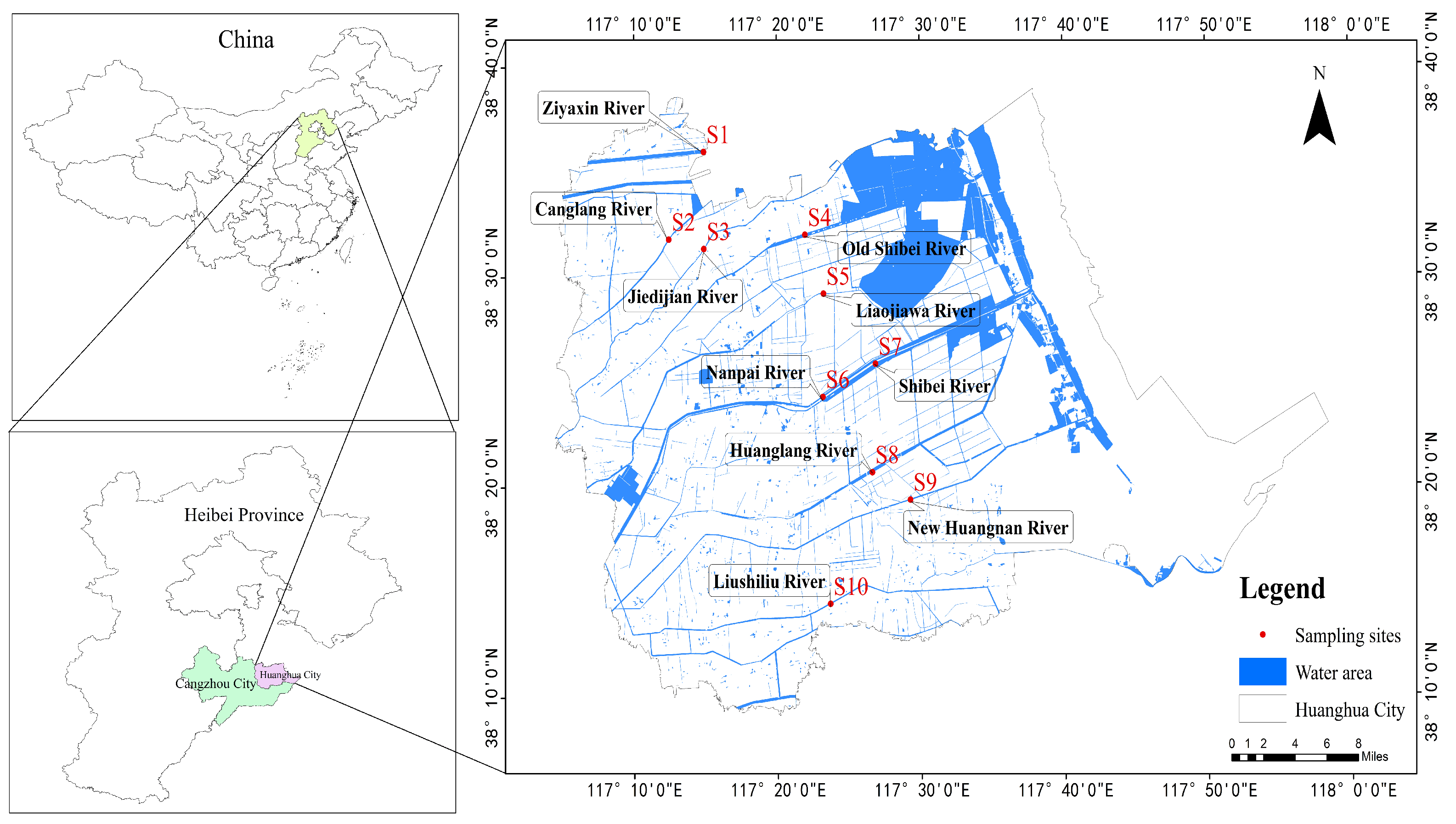
Huanghua City is located in the southeastern region of Hebei Province, China, between 38°09′ and 38°39′ north latitude and 117°05′ and 117°49′ east longitude. It is a total of 2391 km${}^2$. It serves as a water diversion area for the Yellow River, as well as a significant industrial and port city in the Beijing–Tianjin–Hebei region. In recent years, Huanghua City has seen an increase in the number of fisheries, battery industries, fertilizers, pesticides, and metal workshops. These massive wastewater discharges pose a threat to the ecosystems of inland rivers and the Bohai Sea. Water resource safety is inextricably linked to Huanghua City’s local economic and social development as the Yellow River receiving area. The location of the study area is shown in Figure 1.

2.2. Sample Collection and Processing

Ten sediment samples were collected from ten different locations in Huanghua City in July 2018. Each sampling site’s location (latitude and longitude) was determined by GPS (Figure 1). Approximately 10 cm of surface sediment was collected using a column sediment sampler, then approximately 1 kg of sediment was collected into clean polyethylene bags and processed immediately upon return to the laboratory. Samples were stored in the laboratory at a low temperature of −20 °C. Wet samples were extracted from each piece to determine moisture content, and the remaining sediment samples were dried under natural conditions. After removing the debris and gravel, samples were screened with a 2 mm mesh nylon sieve. Then, approximately 0.5 g of soil sample was weighed and further ground with an agate mortar, then screened with a 100 mesh nylon sieve. Next, 1 g of the treated sediment samples were digested with $HCl{O}_4-HN{O}_3-HF$. Samples were measured according to the Soil Environmental Quality Standards of China (GB36600-2018, GB15618-2018) [15,16]. The concentrations of Cu, Zn, and Pb in the extracts were determined with atomic emission spectroscopy with inductively coupled plasma (ICP-AES Prodigy7). The concentrations of As and Hg in the extracts were determined using an atomic fluorescence spectrometer (AFS-230E). The accuracy of the analytical procedures used to analyze metals in sediments was checked using the Chinese certified stream sediment reference material (GBW07312 (GSD-12)), and good agreement with the certified values was obtained. The concentrations of the studied metals in sediment are shown in Table 1. In addition, arsenic is not a metallic element, but the properties of arsenic are similar to HMs. Thus, most studies on HM include arsenic [1,2,9].

2.3. Coefficients of Variation

The coefficient of variation measures the degree of dispersion of a dataset. The coefficient of variation is the ratio of the standard deviation to the mean. The greater the coefficient of variation, the greater the spatial dispersion of HM concentrations, and the greater the impact of external influences on HMs. With coefficients of variation above 20%, human activities are the leading cause of spatial variation in HMs [17]. The coefficient of variation is as follows:

$$VC=\frac{Sd}{Av}$$

(1)

where Sd is the standard deviation; Av is the average value.

2.4. Assessment Method

2.4.1. Geoaccumulation Index

Muller (1979) proposed the Geoaccumulation index ($I_{geo}$), which is used to assess HM contamination in sediments. The method calculates the ratio of HM concentration to its geochemical background value to determine the level of HM contamination in the sediment. The geoaccumulation index is as follows:

$$I_{geo}={log}_2\left(\frac{C_i}{K\times B_i}\right)$$

(2)

where $C_i$ is the measured HM (i) concentrations in the sediment; $B_i$ is the geochemical background value of HM (i), as shown in Table 1; K is correction factor due to anthropogenic influences, usually valued at 1.5. Geoaccumulation Index consists of seven grades, shown in Table 2.

2.4.2. Potential Ecological Risk Index

Hakanson (1980) proposed the potential ecological risk index (PER). This method considers not only the environmental impact of a single pollutant but also the integrated impact of multiple pollutants. In addition, potential risk level of HMs can be calculated quantitatively based on both toxic effects and sensitive conditions of HMs. The following equations are used to calculate $RI$ and $E_r$:

$$C_f^i=\frac{C_s^i}{C_n^i}$$

(3)

$$E_r^i=\frac{T_r^i}{C_f^i}$$

(4)

$$RI=\sum _{i=1}^n{E}_r^i$$

(5)

where $C_f^i$ is the pollution coefficient; $C_s^i$ is the determined HM (i) concentration; $C_n^i$ is the geochemical background value of HM (i) in sediments; $T_r^i$ is the toxicity coefficient, as shown in Table 1; $E_r^i$ is the individual potential ecological risk index of HM (i); and RI represents the general potential ecological risk index of HM (i), which is the sum of all risk index for HMs. The values of $E_r^i$ can be classified into five categories, and RI values can be classified into four categories, as shown in Table 2.

2.4.3. Sediment Quality Guidelines

The sediment quality guidelines (SQG) demonstrate the relationship between the measured HM concentrations and mortality of biological organisms [18]. To evaluate the potential biotoxic effects of HMs, this method employs two sets of indicators: the threshold effect level (TEL) and the probable effect level (PEL), as well as the effects range low (ERL) and the effects range median (ERM). The potential biotoxic effects were assessed in this study using two guideline values: ERL and ERM. (1) The HM concentration is lower than the ERL values, and the adverse bio-toxic effects are rare. (2) The HM concentration is higher than the ERM values, and the adverse bio-toxic effect occurs frequently. (3) The HM concentration is between ERL and ERM, and the adverse bio-toxic effect occurs occasionally. The ERL and ERM values are shown in Table 1. The mSQG-Q is a widely used method that was proposed by Long and MacDonald (1998). The equation used to calculate $mERM-Q$ is given below:

$$mERM-Q=\sum _{i=1}^n\left(\frac{C_i}{ER{M}_i\times n}\right)$$

(6)

where $C_i$ is the measured HM (i) concentrations in sediments (mg/kg); n is the number of HM; and $ER{M}_i$ is the ERM of HM (i) (mg/kg). The possible bio-toxic effects in sediments can be classified into four categories, as shown in Table 2.

Table 1. Statistical summary of the concentration of studied metals in sediment, geochemical background values ($B_i$), toxicity coefficients ($T_r^i$), ERL, and ERM.

	Cu (mg/kg)	Zn (mg/kg)	As (mg/kg)	Hg (mg/kg)	Pb (mg/kg)	References
S1	45.28	112.33	9.18	0.045	42.38	This study
S2	61.07	79.68	12.69	0.039	29.37
S3	53.21	59.18	13.72	0.021	12.38
S4	44.22	98.57	32.69	0.108	10.07
S5	87.02	157.36	9.07	0.032	58.14
S6	71.33	74.35	21.01	0.087	41.39
S7	30.28	125.31	9.69	0.025	34.25
S8	41.95	87.35	12.08	0.102	12.68
S9	81.39	49.25	10.36	0.112	33.01
S10	53.57	98.85	8.36	0.024	21.07
$B_i$	21.8	78.4	13.6	0.04	21.5	[19]
$T_r^i$	5	1	10	40	5	[1]
ERL	34	150	8.2	0.15	46.7	[20]
ERM	270	410	70	0.71	218	[21]

Table 1. Statistical summary of the concentration of studied metals in sediment, geochemical background values ($B_i$), toxicity coefficients ($T_r^i$), ERL, and ERM.

	Cu (mg/kg)	Zn (mg/kg)	As (mg/kg)	Hg (mg/kg)	Pb (mg/kg)	References
S1	45.28	112.33	9.18	0.045	42.38	This study
S2	61.07	79.68	12.69	0.039	29.37
S3	53.21	59.18	13.72	0.021	12.38
S4	44.22	98.57	32.69	0.108	10.07
S5	87.02	157.36	9.07	0.032	58.14
S6	71.33	74.35	21.01	0.087	41.39
S7	30.28	125.31	9.69	0.025	34.25
S8	41.95	87.35	12.08	0.102	12.68
S9	81.39	49.25	10.36	0.112	33.01
S10	53.57	98.85	8.36	0.024	21.07
$B_i$	21.8	78.4	13.6	0.04	21.5	[19]
$T_r^i$	5	1	10	40	5	[1]
ERL	34	150	8.2	0.15	46.7	[20]
ERM	270	410	70	0.71	218	[21]

Table 2. The classification of indices.

Indices	Classification	Contamination Degree	References
$I_{geo}$	$I_{geo}\le 0$	Unpolluted	[22]
	$0<I_{geo}\le 1$	Slightly polluted
	$1<I_{geo}\le 2$	Moderately polluted
	$2<I_{geo}\le 3$	Moderately to strongly polluted
	$3<I_{geo}\le 4$	Strongly polluted
	$4<I_{geo}\le 5$	Strongly to extremely polluted
	$I_{geo}>5$	Extremely polluted
PER	$E_r^i<40$	Low risk	[1]
	$40\le E_r^i<80$	Moderate risk
	$80\le E_r^i<160$	Considerable risk
	$160\le E_r^i<320$	High risk
	$E_r^i\ge 320$	Extremely high risk
	$RI<150$	Low risk
	$150\le RI<300$	Moderate risk
	$300\le RI<600$	Considerable risk
	$RI\ge 600$	High risk
SQG	$mERM-Q\le 0.1$	$9\%$ bio-toxic effects	[23]
	$0.1<mERM-Q\le 0.5$	$21\%$ bio-toxic effects
	$0.5<mERM-Q\le 1.5$	$49\%$ bio-toxic effects
	$mERM-Q>1.5$	$76\%$ bio-toxic effects

Table 2. The classification of indices.

Indices	Classification	Contamination Degree	References
$I_{geo}$	$I_{geo}\le 0$	Unpolluted	[22]
	$0<I_{geo}\le 1$	Slightly polluted
	$1<I_{geo}\le 2$	Moderately polluted
	$2<I_{geo}\le 3$	Moderately to strongly polluted
	$3<I_{geo}\le 4$	Strongly polluted
	$4<I_{geo}\le 5$	Strongly to extremely polluted
	$I_{geo}>5$	Extremely polluted
PER	$E_r^i<40$	Low risk	[1]
	$40\le E_r^i<80$	Moderate risk
	$80\le E_r^i<160$	Considerable risk
	$160\le E_r^i<320$	High risk
	$E_r^i\ge 320$	Extremely high risk
	$RI<150$	Low risk
	$150\le RI<300$	Moderate risk
	$300\le RI<600$	Considerable risk
	$RI\ge 600$	High risk
SQG	$mERM-Q\le 0.1$	$9\%$ bio-toxic effects	[23]
	$0.1<mERM-Q\le 0.5$	$21\%$ bio-toxic effects
	$0.5<mERM-Q\le 1.5$	$49\%$ bio-toxic effects
	$mERM-Q>1.5$	$76\%$ bio-toxic effects

2.5. Identifying Driving Factors Affecting Pollution Sources

2.5.1. Positive Matrix Factorization Model

The PMF model, first proposed by Patero et al. in 1994, is a source apportionment method based on an analytical factoring technique [24]. It uses the limitation of non-negative source contributions to overcome the classical multivariate approach limitations [2]. In this study, PMF 5.0 was used to analyze HM pollution sources. An original matrix $x_{ij}$ is decomposed by the model into a residual matrix ($e_{ij}$) and two factor matrices ($g_{ik}$ and $f_{kj}$). The equations are shown below:

$$x_{ij}=\sum _{k=1}^{p}gik{f}_{kj}+e_{ij}$$

(7)

where $x_{ij}$ is the HM (j) concentration in sample (i); p is the number of factors; $g_{ik}$ is factor contribution of the source (k) to sample (i); $f_{kj}$ is the contribution of source (k) to HM (j); and $e_{ij}$ is calculated from an objective function Q with a minimum value.

$$Q=\sum _{i=1}^n\sum _{j=1}^m{\left(\frac{x_{ij}}{u_{ij}}\right)}^2$$

(8)

$$u_{ij}=\sqrt{{\left(EF{x}_{ij}\right)}^2+{\left(0.5MDL\right)}^2}$$

(9)

$$u_{ij}=0.1x_{ij}+\frac{MDL}{3}$$

(10)

where $u_{ij}$ refers to the uncertainty of HM (j) in sample (i); MDL is the method detection limit. There are two methods evaluated for uncertainty. After several combinations of calculations, five HMs were suitable for Formula (10).

2.5.2. RDA Analysis

RDA was used to explore the correlation between explanatory variables and response variables. In this paper, agricultural production potential (APP), population density (PD), GDP, land utilization including dryland (DL), woodland (WL), water area (WA), residential land (RL), and industrial construction (IC) are regarded as explanatory variables. The concentrations of HMs are considered as response variables. Regional land utilization data were collected and interpreted using Landsat 8 remote sensing imagery (30 m resolution). According to the land utilization current state classification standard, the land types are divided into 25 secondary types and 6 primary types: cultivated land, woodland, grassland, water, residential and construction land, and unused land. PD based on 100 m resolution data, and 1 km resolution data for other explanatory variables were from the Resource and Environment Science and Data Center (https://www.resdc.cn/, accessed on 10 November 2022). Different scales of land utilization within the 200 m–10 km buffer zone have been shown to have significant effects on the water environment of rivers and lakes [25]. Therefore, a buffer zone of 3 km was delineated with the sampling sites as the center, and the area ratio of explanatory variables within the buffer zone was calculated by zonal statistics as the table in GIS. The result of area ratio of each factor is shown in

Table 3. Area ratio of each factor.

	DL	WL	WA	RL	IC	APP	PD	GDP
S1	0.8033	0.0000	0.0427	0.0886	0.0019	0.0769	0.0136	0.0000
S2	0.8861	0.0199	0.0183	0.0757	0.0000	0.2778	0.0109	0.0000
S3	0.8487	0.0000	0.0202	0.1257	0.0023	0.0000	0.0000	0.0000
S4	0.8567	0.0000	0.0693	0.0512	0.0229	0.6571	0.0000	0.0000
S5	0.7431	0.0000	0.0319	0.2250	0.0000	0.0968	0.0617	0.4231
S6	0.8158	0.0000	0.0451	0.1337	0.0054	0.0000	0.0391	0.6000
S7	0.8965	0.0000	0.0345	0.0690	0.0000	0.0000	0.0000	0.1852
S8	0.8650	0.0000	0.0103	0.0746	0.0171	0.0000	0.0000	0.0000
S9	0.7867	0.0000	0.0029	0.0532	0.1573	0.0370	0.0000	0.0000
S10	0.8930	0.0041	0.0000	0.1005	0.0024	0.1250	0.0000	0.0000

.

2.6. Statistical Tools

SPSS 26.0 was used to compute the means of the HM concentrations in sediments and the variation coefficients. The EPA PMF 5.0 software recommended by the US Environmental Protection Agency was used to analyze the sources of HM pollution. RDA was used to explore driving factors affecting pollution sources by Canoco 5.0. Other calculations were performed by Microsoft Excel. The spatial distribution results were presented by ArcMap 10.7, and the level of pollution was presented by Origin 2021.

3. Results and Discussion

3.1. Heavy Metal Concentration in Sediment

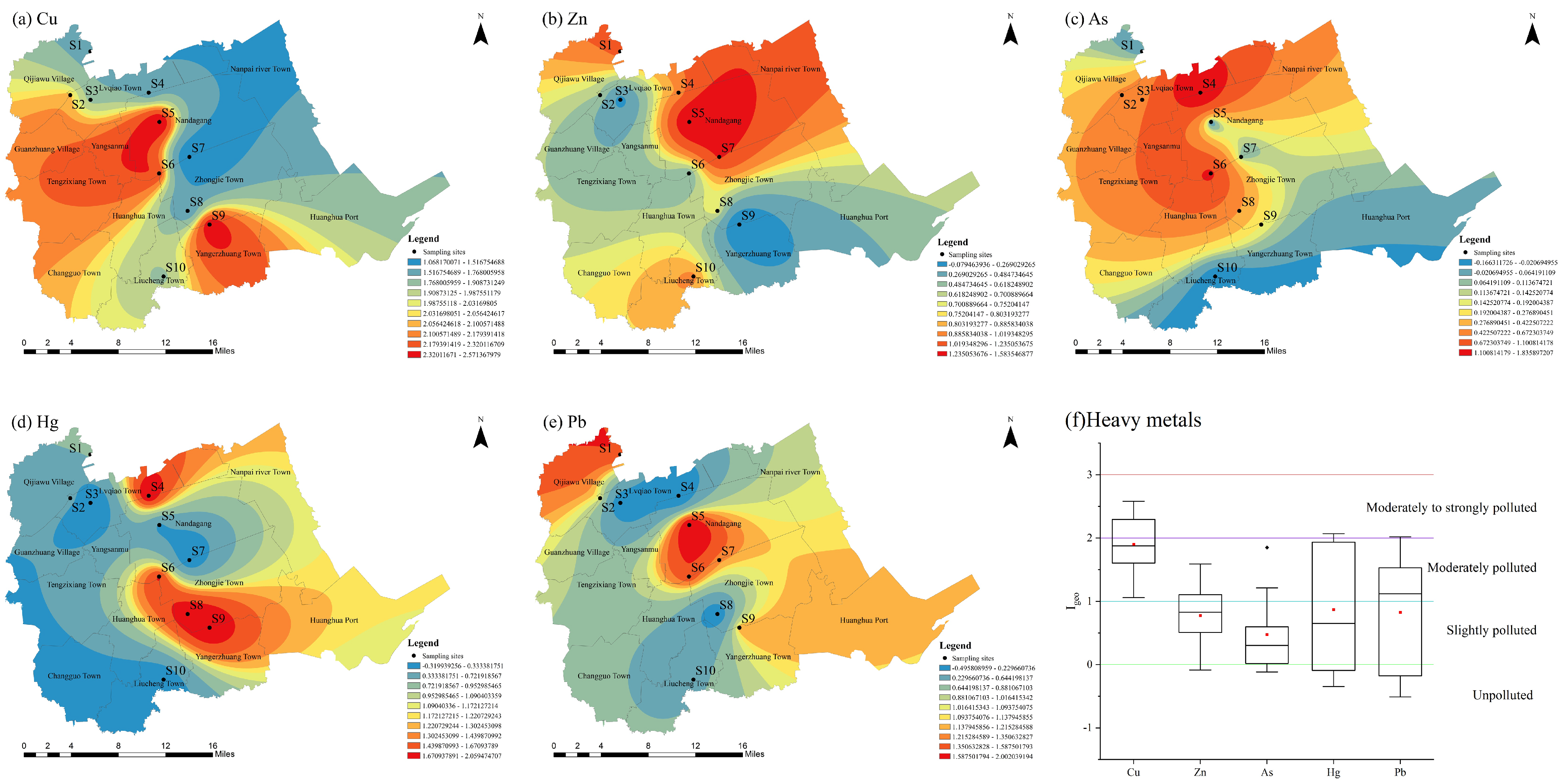
The spatial distribution of HM concentrations was obtained by RBF interpolation at 10 sampling sites using Arcgis spatial analysis tool. The highest Cu values were found in central Huanghua City, as shown in Figure 2a–e. The elements Zn and As were found in higher concentrations in the northern sides of the city and in lower concentration in the south. Areas S4 and S9 had higher Hg concentrations of 0.108 and 0.112, respectively. Pb concentration was lowest overall, with the highest values concentrated in the city’s center. As shown in Figure 2f, the mean HM concentrations in the sediment from 10 sites in Huanghua City were Zn (94.223 mg/kg) > Cu (56.932 mg/kg) > Pb (29.474 mg/kg) > As (13.885 mg/kg) > Hg (0.0595 mg/kg), with the mean values of HMs all being higher than the geochemical background values. Cu, Zn, As, Hg, and Pb concentrations were higher than the geochemical background values at 100%, 60%, 20%, 50%, and 60% the sites, respectively. This result indicated that all HMs were contaminated to some extent.

The concentrations of Zn and Cu were higher in Huanghua City. Spatially, a wide range of values for Cu were present in the whole city. The highest concentrations of Zn and As were found in the north, whereas the lowest concentrations were found in the south. Hg and Pb were lower throughout the study area, with the former being highest on the southern side of the city and the latter being the highest at the center.

Cu, Zn, As, Hg, and Pb had coefficients of variation that exceeded 20% (31.99%, 33.98%, 54.48%, 63.85%, and 52.89%, respectively), indicating that human factors influenced HM pollution in sediments [22].

3.2. Heavy Metal Pollution Assessment

3.2.1. Heavy Metal Pollution Status

The spatial distributions of $I_{geo}$ are shown in Figure 3a–e. The highest $I_{geo}$ values for Cu were found in central Huanghua City, in the moderately to strongly polluted category. The highest $I_{geo}$ values for Zn and As were found in the north, which fell into the moderately polluted category, whereas the south showed low values. The highest values for Hg were in the northern part of the city, and the highest values for Pb were in the center; both were in the moderately to strongly polluted category. However, the contaminated areas for Hg and Pb were small. The order of the mean $I_{geo}$ for the HMs in sediments was Cu(1.902) > Hg(0.871) > Pb(0.827) > Zn(0.774) > As(0.475), among which Cu belonged to moderately polluted, whereas other HMs belonged to slightly polluted, as shown in Figure 3f.

Cu had the highest level of contamination. A wide variety of $I_{geo}$ values for Cu were displayed spatially. Although Zn and As were widely contaminated, they fell into the low polluted category. In contrast, the contaminated areas for Hg and Pb were small, but the level of pollution was higher. Low regional variation existed between HM concentrations and their levels of contamination. The geoaccumulation index method has the advantages of requiring fewer data and having a shorter evaluation process. It reflects the natural variation of HM pollution. However, toxicity and adverse effects on organisms are not taken into account.

3.2.2. Potential Ecological Risk Assessment

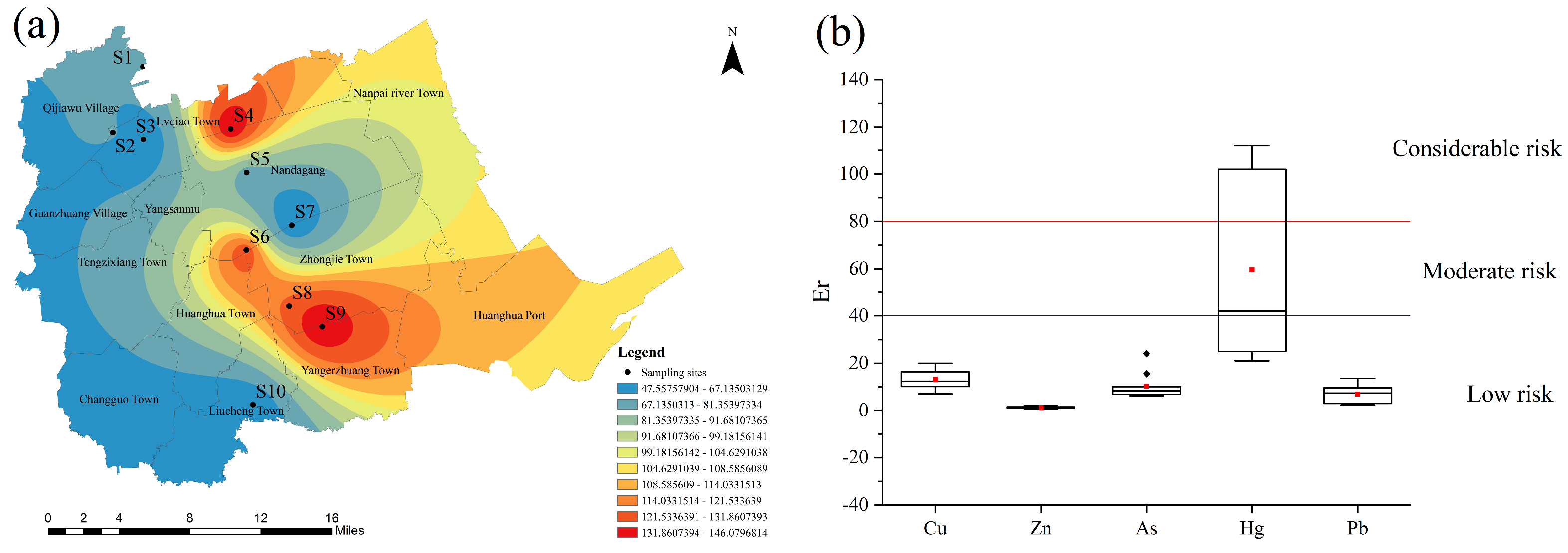
Figure 4a shows the spatial distributions of the general potential ecological risk index. The northern and southern parts of the city had higher RI values while posing little risk. Hg posed the highest risk. As shown in Figure 4b, the average Er of 10 sampling sites in descending order was Hg(59.500) > Cu(13.058) > As(10.210) > Pb(6.854) > Zn(1.202), among which Hg was a moderate risk, and other HMs were low risks.

Hg had the most serious potential ecological risk. Spatially, the high values of RI were mainly distributed in the south. The spatial heterogeneity between RI and the geoaccumulation index of Hg was low, indicating that the advantages of the potential ecological risk evaluation method take into account the toxic effects. However, the effects of different HMs are not regarded when calculating the comprehensive effect of HMs.

3.2.3. Bio-Toxic Risk Assessment

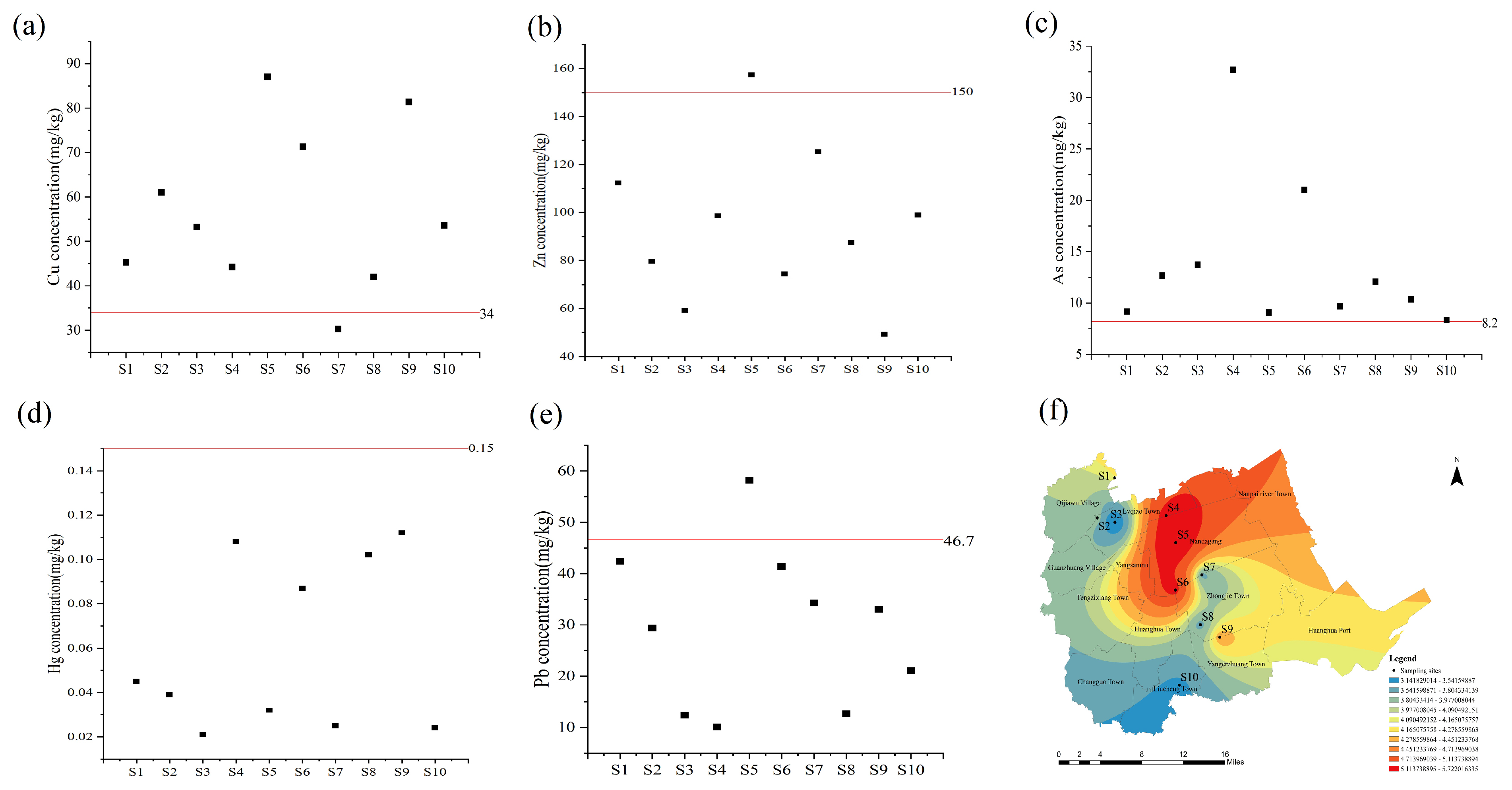
The sediment quality guidelines method focuses more on the biological effects of various contaminants in sediments. It reflects the critical level of aquatic organisms in contact with the sediment that is harmed by HMs. Cu and As concentrations at most sites were between ERL and ERM, indicating that adverse bio-toxic effects occurred occasionally. Other HMs concentrations at most sites were below the ERL, indicating that adverse bio-toxic effects rarely occur. This is shown in Figure 5a–e. A wide range of Huanghua City is a bio-toxic risk, as well as 76% possibly being poisoned. The highest mERM-Q values were found in the north, as can be seen in Figure 5f.

The bio-toxic effects of Cu and As were higher. Spatially, Huanghua City had 76% bio-toxic effects, and the highest mERM-Q values were shown in the north.

3.3. Source Interpretation with PMF and RDA

3.3.1. Source Classification Based on PMF Model

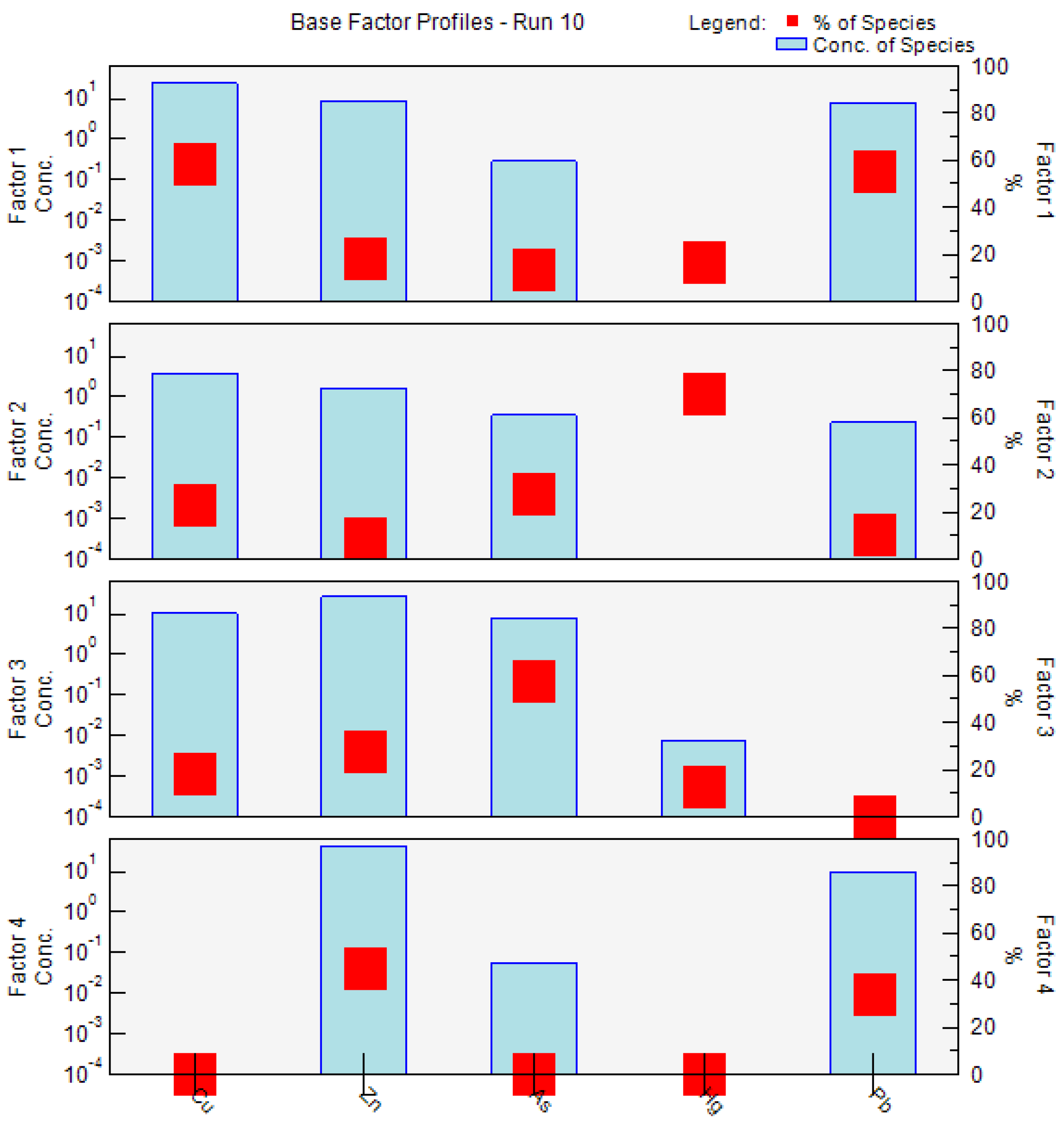
The results of the potential ecological risk assessment and bio-toxic risk assessment revealed that HM pollution had multiple sources in sediments. In this paper, we used the PMF model to explore the contribution of each HM and each sampling site to the pollution source, which helps to identify the sources of HM pollution in the sediment. Three to four factors were selected until the values of $Q_{Robust}$ and $Q_{Ture}$ were closest to ensure the precision of the model. The number of runs was 20, all HMs were classified as “strong” (S/N > 1) during the identification process, and almost all of the residuals were between −3 and 3. The $R^2$ values for Cu, Zn, As, Hg, and Pb were 0.90, 0.92, 0.97, 0.99, and 0.94, respectively. The S/N values for Cu, Zn, As, Hg, and Pb were 9.0, 9.0, 9.0, 7.6, and 8.9, respectively. The $R^2$ values were all higher than 0.9, and the signal-to-noise ratio (S/N) was higher than 5.70, indicating a good model fit [2]. Figure 6 shows the factor profile and contribution rates of various HMs in the study area. There are four HM pollution sources. Factor 1 mainly explained the Cu and Pb (contributions were 58.5%, and 55.8%, respectively), factor 2 had the highest contribution of Hg (contribution was 70.2%), factor 3 had the strongest contribution with As (contribution was 58.2%), and factor 4 had the highest contribution of Zn (contribution was 44.9%).

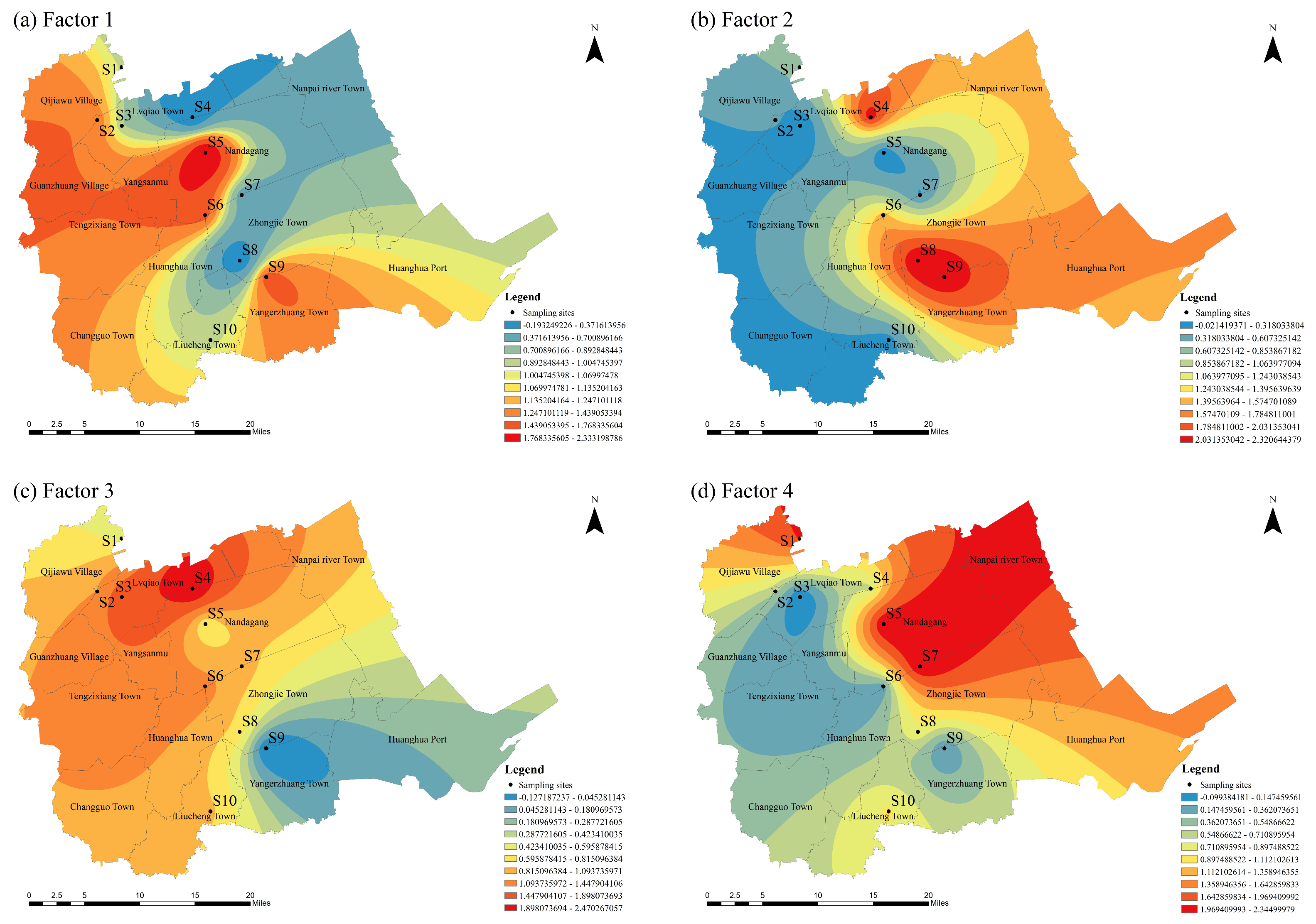
Moreover, the contribution of sampling site to pollution source was also calculated by the PMF model. We explored the spatial distribution characteristics of pollution sources using RBF interpolation in the Arcgis spatial analysis tool, which helps to propose control measures for different regions. Figure 8 shows that factor 1, factor 2, and factor 3 had the highest contribution values in the central, southern, and northern areas of the city, respectively. The highest contribution values for factor 4 occurred in the central and northern areas. Therefore, the driving factors affecting these pollution sources are different. The factors will be discussed further in the following section.

3.3.2. Driving Factors Affecting Pollution Sources Based on RDA Anaylsis

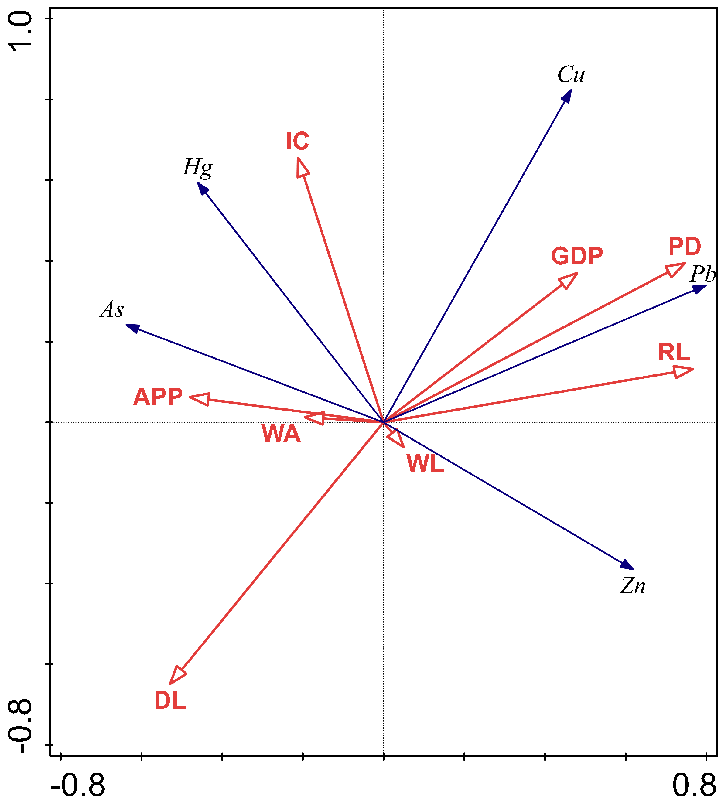
For the linear model RDA, the larger the length of the projection vector of the data in a certain direction, the higher the correlation. The arrows in the same direction indicate a positive correlation between the data, and the reverse means a negative correlation. RDA can clearly reflect the correlation between explanatory variables and response variables. Impact of human activities on sediment HM pollution are to be considered. Here we discuss the effects of APP, PD, GDP, and land utilization on HM concentration. Therefore, the GIS, PMF model, and RDA were combined to explore the driving factors affecting pollution sources and spatial distribution of sources. The results of RDA are shown in Figure 7.

Cu and Pb are in the first category. RDA revealed a positive correlation between RL, Cu, and Pb. Previous studies had shown that coal combustion is the primary source of Cu and Pb pollution, and most of China’s energy supply comes from coal combustion, which is the identified element of motor vehicle pollution sources, influenced by industrialization and urbanization [26,27]. Pb was strongly positively correlated with PD, which indicated Pb pollution was more serious in places with high population density and heavy traffic, whereas Cu was strongly positively correlated with GDP, which indicated Cu pollution was also slightly influenced by industry. From Figure 8, it can be seen that traffic pollution has a more critical influence on factor 1 compared with industrial pollution in the central part of Huanghua City. In the future, the government should consider reducing the pollution caused by vehicle emissions by promoting low-carbon travel, building green belts, etc.

The second category is Hg. RDA revealed a positive correlation between IC and Hg. Metallurgy, electronics, electroplating, and other industrial activities lead to Hg pollution [28]. Hg was positively correlated with WA; this may be caused by industrial wastewater discharges that have adversely affected the water quality of nearby rivers. From Figure 8, it can be seen that factor 2 represented industrial wastewater discharges in the southern part of Huanghua City. The underdevelopment of chemical equipment and technology led to industrial wastewater discharges with excessive Hg concentration [29]. Therefore, we suggest improving metal smelting technology while increasing the regulation of industrial wastewater discharge.

The third category is As. RDA revealed that As has a high positive correlation with WA and APP. Some studies showed that it is mainly caused by wastewater discharged from agricultural production; long-term mass application of pesticides with high As content, such as calcium arsenate, lead arsenate, sodium arsenite, disodium methyl arsenate, phosphorus fertilizers, and other As-containing fertilizers, in agricultural production activities causes As to accumulate in the environment. Eventually, a large amount of As enters rivers and lakes through rainfall [30]. From Figure 8, it can be seen that factor 3 represented farmland drainage water in the northern part of Huanghua City. The Ministry of Agriculture needs to strictly control the HM content of fertilizer products and improve the fertilizer quality to prevent HMs and other harmful substances in fertilizers from entering the environment.

The fourth category is Zn. RDA revealed that WL and Zn had a significantly positive correlation, which indicated that Zn may be influenced by the natural geological background and soil parent materials of the river [31]. From Figure 8, it can be seen that factor 4 represented the natural origin in the northeastern part of Huanghua City.

4. Conclusions

Human activities are important sources of HM pollution in the sediment and they cannot be ignored. Different human activities have different impacts on ecological risks from various aspects. For this study area, the impacts of RL, PD, and IC on ecological risks are worth taking into account.

The results revealed that the highest degree of natural pollution was Cu, and the source mainly comes from traffic pollution (factor 1). The combination of RDA and GIS mapping confirmed that RL, PD, GDP, and IC had a main influence on factor 1 in the central part of Huanghua City, thus we suggest low-carbon travel and building green belts around industrial regions and roads; the highest level of potential ecological risk was Hg, and the pollution is mainly caused by industrial wastewater discharges (factor 2). IC had a main influence on factor 2 in the southern part of the city, thus we suggest improving metal smelting technology and preventing untreated industrial wastewater from being discharged into surrounding rivers; the highest effects of bio-toxic risk was As, and the source mainly comes from farmland drainage water (factor 3). APP and WA had a main influence on factor 3 in the northern part of the city, thus we suggest strictly controlling the HM concentration of fertilizer products to prevent HMs from being discharged into surrounding rivers. Zn might be of natural origin (factor 4), and WL has high contribution to factor 4.

The evaluation of sediment HM pollution should focus on understanding the ecological hazards of HMs from different aspects. Based on human activities on the banks, it is crucial to propose targeted treatment measures for sediment pollution for different HMs and regions. This method we proposed offers a new idea for quantification of pollution sources and system control of sediment HM pollution in Huanghua City.

References

- Liu, B.; Xu, M.; Wang, J.; Wang, Z.; Zhao, L. Ecological risk assessment and heavy metal contamination in the surface sediments of Haizhou Bay, China. Mar. Pollut. Bull. 2021, 163, 111954. [Google Scholar] [CrossRef] [PubMed]
- Proshad, R.; Uddin, M.; Idris, A.M.; Al, M.A. Receptor model-oriented sources and risks evaluation of metals in sediments of an industrial affected riverine system in Bangladesh. Sci. Total Environ. 2022, 838, 156029. [Google Scholar] [CrossRef] [PubMed]
- Liao, J.; Cui, X.; Feng, H.; Yan, S. Environmental Background Values and Ecological Risk Assessment of Heavy Metals in Watershed Sediments: A Comparison of Assessment Methods. Water 2021, 14, 51. [Google Scholar] [CrossRef]
- Chen, Q.; Huang, F.; Cai, A. Spatiotemporal Trends, Sources and Ecological Risks of Heavy Metals in the Surface Sediments of Weitou Bay, China. Int. J. Environ. Res. Public Health 2021, 18, 9562. [Google Scholar] [CrossRef] [PubMed]
- Gu, Y.; Gao, Y. An unconstrained ordination- and GIS-based approach for identifying anthropogenic sources of heavy metal pollution in marine sediments. Mar. Pollut. Bull. 2019, 146, 100–105. [Google Scholar] [CrossRef]
- Yin, Z.; Song, L.; Song, H.; Hui, K.; Lin, Z.; Wang, Q.; Xuan, L.; Wang, Z.; Gao, W. Remediation of copper contaminated sediments by granular activated carbon-supported titanium dioxide nanoparticles: Mechanism study and effect on enzyme activities. Sci. Total Environ. 2020, 741, 139962. [Google Scholar] [CrossRef]
- Ma, T.; Zhang, Y.; Hu, Q.; Han, M.; Li, X.; Zhang, Y.; Li, Z.; Shi, R. Accumulation Characteristics and Pollution Evaluation of Soil Heavy Metals in Different Land Use Types: Study on the Whole Region of Tianjin. Int. J. Environ. Res. Public Health 2022, 19, 13. [Google Scholar] [CrossRef]
- Anbuselvan, N.D.S.N.; Sridharan, M. Heavy metal assessment in surface sediments off Coromandel Coast of India: Implication on marine pollution. Mar. Pollut. Bull. 2018, 131, 712–726. [Google Scholar] [CrossRef]
- Yang, H.; Jeong, H.; Bong, K.; Jin, D.; Kang, T.; Ryu, H.; Han, J.; Yang, W.; Jung, H.; Hwang, S. Organic matter and heavy metal in river sediments of southwestern coastal Korea: Spatial distributions, pollution, and ecological risk assessment. Mar. Pollut. Bull. 2020, 159, 111466. [Google Scholar] [CrossRef]
- Abu-Zied, R.H.; Al-Mur, B.A.; Orif, M.I.; Al Otaibi, A.; Ghandourah, M.A. Concentration distribution, enrichment and controlling factors of metals in Al-Shuaiba Lagoon sediments, Eastern Red Sea, Saudi Arabia. Environ. Earth Sci. 2021, 80, 385. [Google Scholar] [CrossRef]
- Ahmadov, M.; Humbatov, F.; Mammadzada, S.; Balayev, V.; Ibadov, N.; Ibrahimov, Q. Assessment of heavy metal pollution in coastal sediments of the western Caspian Sea. Environ. Monit. Assess. 2020, 192, 500. [Google Scholar] [CrossRef]
- Zhao, Z.; Hao, M.; Li, Y.; Li, S. Contamination, sources and health risks of toxic elements in soils of karstic urban parks based on Monte Carlo simulation combined with a receptor model. Sci. Total Environ. 2022, 839, 156223. [Google Scholar] [CrossRef]
- Anaman, R.; Peng, C.; Jiang, Z.; Liu, X.; Zhou, Z.; Guo, Z.; Xiao, X. Identifying sources and transport routes of heavy metals in soil with different land uses around a smelting site by GIS based PCA and PMF. Sci. Total Environ. 2022, 823, 153759. [Google Scholar] [CrossRef]
- Souto-Oliveira, C.E.; Kamigauti, L.Y.; Andrade, M.d.F.; Babinski, M. Improving Source Apportionment of Urban Aerosol Using Multi-Isotopic Fingerprints (MIF) and Positive Matrix Factorization (PMF): Cross-Validation and New Insights. Front. Environ. Sci. 2021, 9, 623915. [Google Scholar] [CrossRef]
- Ministry of Ecology and Environment. Soil Environmental Quality Risk Control Standard for Soil Contamination of Agricultural Land; Ministry of Ecology and Environment: Beijing, China, 2018.
- Ministry of Ecology and Environment. Soil Environmental Quality Risk Control Standard for Soil Contamination of Development Land; Ministry of Ecology and Environment: Beijing, China, 2018.
- Bai, D.; Zhang, T.; Bao, J.; Chen, T.; Wang, H.; Jin, X.; Jin, J.; Yang, T. Pollution Distribution and Ecological Risk Assessment of Heavy Metals in River Sediments from the Ancient Town of Suzhou. Environ. Sci. 2021, 42, 3206–3214. [Google Scholar] [CrossRef]
- Bakak, Ö.; Küçüksezgin, F.; Özel, F.E. Assessment of element concentrations in surface sediment samples from Sığacık Bay (eastern Aegean). Turk. J. Earth Sci. 2020, 29, 1154–1166. [Google Scholar] [CrossRef]
- Zang, L.; Zhang, G.; Zhang, H.; Zhu, Y. Assessment on Spatial Variabilty and Pollution of the Heavy Metal in Soil of Huanghua City. Res. Soil Water Conserv. 2017, 24, 337–342. [Google Scholar] [CrossRef]
- Zhao, Y.; Dong, X.; Wang, L.; Qi, Y.; You, L.; Sun, S.; Ma, Y. Selection and comparison of different methods for ecological risk assessment of heavy metals in marine sediments of Laizhou Bay. Mar. Sci. Bull. 2019, 38, 353–360. [Google Scholar] [CrossRef]
- Zhang, Y.; Song, Y.; Wang, L.; Wang, N.; Tian, J.; Ma, Z.; Song, L.; Wu, J. The Ecological Risk Assessment of Heavy Metals in Sediments in Jinzhou Bay, Liaoning Province. Fish. Sci. 2011, 30, 156–159. [Google Scholar] [CrossRef]
- Gao, B.; Zhou, H.; Huang, Y.; Wang, Y.; Gao, J.; Liu, X. Characteristics of heavy metals and Pb isotopic composition in sediments collected from the tributaries in three Gorges Reservoir, China. Sci. World J. 2014, 2014, 685834. [Google Scholar] [CrossRef] [Green Version]
- Liao, J.; Chen, J.; Ru, X.; Chen, J.; Wu, H.; Wei, C. Heavy metals in river surface sediments affected with multiple pollution sources, South China: Distribution, enrichment and source apportionment. J. Geochem. Explor. 2017, 176, 9–19. [Google Scholar] [CrossRef]
- Jia, L.; Liang, H.; Fan, M.; Wang, Z.; Guo, S.; Chen, S. Spatial Distribution Characteristics and Source Appointment of Heavy Metals in Soil in the Areas Affected by Non-Ferrous Metal Slag Field in the Dry-Hot Valley. Appl. Sci. 2022, 12, 9475. [Google Scholar] [CrossRef]
- Song, J.; Zhang, X.; Jiang, D.; Zhao, C.; Li, P. Impact of Land Use Types at Different Scales on Surface Water Environment Quality and Its Driving Mechanism. Environ. Sci. 2022, 43, 3016–3026. [Google Scholar] [CrossRef]
- Guo, G.; Li, K.; Zhang, D.; Lei, M. Quantitative source apportionment and associated driving factor identification for soil potential toxicity elements via combining receptor models, SOM, and geo-detector method. Sci. Total Environ. 2022, 830, 154721. [Google Scholar] [CrossRef]
- Hong, N.; Yang, B.; Tsang, D.C.W.; Liu, A. Comparison of pollutant source tracking approaches: Heavy metals deposited on urban road surfaces as a case study. Environ. Pollut. 2020, 266, 115253. [Google Scholar] [CrossRef]
- Huang, F.; Xu, Y.; Tan, Z.; Wu, Z.; Xu, H.; Shen, L.; Xu, X.; Han, Q.; Guo, H.; Hu, Z. Assessment of pollutions and identification of sources of heavy metals in sediments from west coast of Shenzhen, China. Environ. Sci. Pollut. Res. Int. 2018, 25, 3647–3656. [Google Scholar] [CrossRef]
- Chen, H.; Wang, L.; Hu, B.; Xu, J.; Liu, X. Potential driving forces and probabilistic health risks of heavy metal accumulation in the soils from an e-waste area, southeast China. Chemosphere 2022, 289, 133182. [Google Scholar] [CrossRef]
- Agyeman, P.C.; John, K.; Kebonye, N.M.; Ofori, S.; Borůvka, L.; Vašát, R.; Kočárek, M. Ecological risk source distribution, uncertainty analysis, and application of geographically weighted regression cokriging for prediction of potentially toxic elements in agricultural soils. Process. Saf. Environ. Prot. 2022, 164, 729–746. [Google Scholar] [CrossRef]
- Chen, Z.; Xu, J.; Duan, R.; Lu, S.; Hou, Z.; Yang, F.; Peng, M.; Zong, Q.; Shi, Z.; Yu, L. Ecological Health Risk Assessment and Source Identification of Heavy Metals in Surface Soil Based on a High Geochemical Background: A Case Study in Southwest China. Toxics 2022, 10, 282. [Google Scholar] [CrossRef]
Figure 1.
Location of study area and sampling sites in Huanghua City.
Figure 2.
HM concentration in the sediment. (a–e) Spatial distributions of HM concentrations. (f) The mean of HM concentrations.
Figure 3.
Results of HM pollution status in the sediment. (a–e) Spatial distributions of . (f) The mean of .
Figure 4.
Results of the potential ecological risk assessment. (a) Spatial distributions of RI. (b) Pollution grades of HM in potential ecological risk assessment.
Figure 5.
Results of bio-toxic risk assessment. (a–e) HMs concentration and the red line is the ERL value. (f) Spatial distribution of mERM-Q.
Figure 6.
Profiles and contributions of sources of the HMs based on the PMF model.
Figure 7.
RDA of driving factors and HM concentration.
Figure 8.
Contribution of ten sites for four factors.