Data Conditioning Modes for the Study of Groundwater Resource Quality Using a Large Physico-Chemical and Bacteriological Database, Occitanie Region, France

Abstract

When studying large multiparametric databases with very heterogeneous parameters (microbiological, chemical, and physicochemical), covering a wide and heterogeneous area, the probability of observing extreme values (Z-score > 2.5) is high. The information carried by these few samples monopolizes a large part of the information conveyed by the entire database. The study of the spatial structure of the data and the identification of the mechanisms responsible for the water quality are then strongly degraded. Data transformation can be proposed to overcome these problems. This study deals with a database of 8110 groundwater analyses (Occitanie region, France), on which the bacteriological load was measured in Escherichia coli and Enterococci, in addition to electrical conductivity, major ions, Mn, Fe, As and pH. Three modes of data conditioning were tested and compared to the treatment with raw data. The results show that log transformation is the best option, revealing a relationship between E. coli content and all the other parameters. By reducing the impact of extreme values without eliminating them, it allowed a concentration of information on the first factorial axes of the PCA, and consequently a better definition of the associated processes. The spatial structure of the principal components and their cartographic representation is improved. The conditioning of the data with the square root function led to an intermediate improvement between the logarithmic transformation and the absence of conditioning. The application of these results should allow a targeted, more efficient, and therefore, less expensive monitoring of water quality by Regional Health Agencies.

1. Introduction

Groundwater is a major source of freshwater for the world’s population and is used for domestic, agricultural and industrial purposes. About one-third of the world’s population, mainly but not only in arid or semi-arid countries relies on groundwater for drinking water [1]. However, this resource is threatened by various types of contamination, such as pathogenic bacteria, toxic metals, hydrocarbons, organic contaminants, pesticides, nanoparticles, microplastics and other emerging contaminants, which present a potential risk to human health and ecological services [2]. Driven by the European Water Framework Directive (WFD) in 2000 [3,4,5], many countries have made the effort to inventory the water resource and monitor the quality of water intended for human consumption [6,7,8,9,10,11,12,13,14]. This directive has only reinforced an initiative that has been carried out for more than 30 years in France, where the information is stored in a database called “Sise-Eaux”, managed by the regional health agencies (https://data.eaufrance.fr/concept/sise-eaux, 20 January 2019 accessed on). The regular updating of this database has generated a volume of data that now enables us to study and spatialize the processes behind the variability in water quality, which offers the possibility of targeted, more effective and less costly management. In this context, and although many parameters are regularly monitored, fecal contamination, detected by the presence of fecal germs, particularly Escherichia Coli and Enterococcus, constitutes the vast majority of cases of non-compliance with water intended for human consumption [15,16,17]. This non-compliance with the drinking water standards, often due to strong contamination, which is, however, rare and punctual, is reflected by extreme values in the databases, i.e., nonnormal distribution. In Geoscience studies, the normality of the distribution is sometimes verified for aspects related to the physics of the environment, such as geophysical studies or spatial variations in water content, etc., but more rarely for aspects of chemical quality [18,19], and even less so for the mechanisms responsible for the bacteriological quality of water. The two latter cases present a large amplitude of spatial variability, ranging from several hundred km (spatial variations linked to large geological structures) to very local variations for certain processes affecting, for example, nitrates with millimetric hot spots, or even smaller ones for the denitrification process. For the wide regions, the diversity of environments and processes involved in groundwater quality can lead to frequency distributions that are far from normal. Each environment may or may not have a normal distribution, but when aggregated, the distribution in the data set is likely to deviate from a normal distribution. The frequency distribution of water characteristics can then be considered as the sum of distributions of different environments, each with its own mean and standard deviation. For studies on a smaller spatial scale, such as for groundwater bodies or up to medium size basins, the spatial variability is generally limited [9,20,21,22,23]. The normality assumption is a prerequisite that does not provide a strong constraint and has little impact on the estimation of uncertainties in the calculations, for example for the mapping of environmental features. This point is usually only addressed by geostatisticians [24]. The assumption of data normality is, therefore, a generally forgotten aspect in the study of mechanisms responsible for the variability of water quality, but in the presence of extreme values, these can mask certain processes, and therefore, alter the analysis that is made of the database.

The aim of this work is to compare different conditioning options for bacteriological and physicochemical groundwater data, to assess the degree of agreement with a normal distribution model, to evaluate the impact of extreme values on the multivariate processing of the data, in particular by Principal Component Analysis, as well as on the study of the spatial structure of the information. In order to ensure a large disparity of environments on a regional scale, the region chosen for the study is the Occitanie region located in southern France. This vast region has the particularity of being astride two large basins (Atlantic and Mediterranean sides), two distinct climatic sectors (Oceanic and Mediterranean), and presenting a varied lithology.

2. Materials and Methods

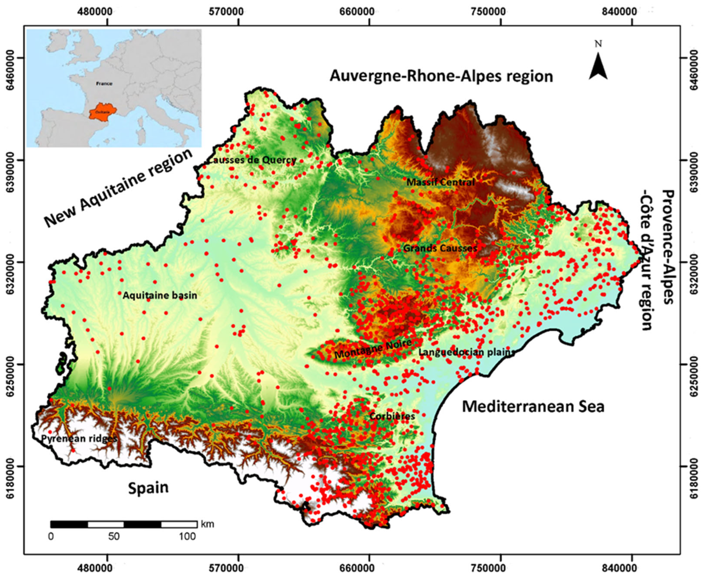
2.1. Study Area

The Occitanie region covers an area of 72,724 km² and has a population of 5.8 million inhabitants. It is bounded to the south by the Mediterranean Sea and the Pyrenean ridgeline, to the east by the Rhône valley, to the north by the Massif Central, and to the west, it covers the upper and middle basin of the Garonne River. It thus straddles two major climatic regions corresponding to its Atlantic side with an oceanic influence (Köppen Cfb, Cwb, Cfc), while its eastern part has a Mediterranean climate (Köppen Csa, Csb). The range of altitudes is very high, from 0 to 3300 m. The lithology is extremely variable, with ancient crystalline basement formations in the Massif Central and the Pyrenees, folded or unfolded sedimentary formations, and recent Languedocian coastal plains. This ensemble covers practically all geological periods with a variety of rocks, namely Cenozoic detrital sedimentary rocks that extend from the Aquitaine basin to the Mediterranean basin, Mesozoic carbonate sedimentary rocks in the Causses, the North Montpellier Garrigues, the Corbières and the Pyrenean foreland, and plutonic, volcanic and sedimentary rocks of varying degrees of metamorphism representing the crystalline massifs (Massif Central, Pyrenees and Montagne Noire).

2.2. Database

The data were extracted from the national SISE-EAUX database, managed by the Regional Health Agencies since 1990, according to the procedure described by Tiouiouine et al. [25]. Due to the management of the database by the Regional Health Agencies, these extractions are necessarily carried out according to the administrative division of the French regions, and in the context of this work, on the whole of the Occitanie region. All analyses were performed by laboratories with international accreditation and certification of analytical quality. The extraction concerned the period of about 11 years, more precisely the data acquired between 22 January 2007 and 18 December 2018. Only the analyses of raw water were kept, i.e., before any treatment. For each water sample taken, several analysis reports could have been realized, namely, complete with several hundreds of parameters, standard with about 30 parameters, or a routine follow-up, with only about ten parameters. The result is a matrix with some empty cells that need to be conditioned before processing. After the manual correction of errors during data entry in the database and the elimination of empty cells, a matrix consisting of 8110 observations and 15 parameters was used for this study. These samples came from 1972 sampling points, i.e., an average of 4.1 samples for each sampling point, and spread over 106 groundwater bodies delimited by the French Geological Survey (BRGM) in the BDLISA database (https://bdlisa.eaufrance.fr/, accessed on 7 February 2022). The selected parameters were Enterococci, E. coli, Electrical Conductivity, Na⁺, Ca²⁺, Mg²⁺, Cl⁻, SO₄²⁻, HCO₃⁻, NO₃⁻, Fe, Mn, As and the pH, which was added after transformation into H⁺ concentration to avoid mixing variables with logarithmic and non-logarithmic units. The detection limit was applied to values below it. In this work, which is based on correlations or frequency distributions, the choice of the unit of the variables does not matter. The concentrations of major ions are in Mole L⁻¹, those of trace elements are in mg L⁻¹, and in units per 100 mL for the bacteriological variables.

All observations are georeferenced and their location is presented in Figure 1. The difference in the density of groundwater collection points can be explained by several factors. The karstic sectors such as the Causses du Quercy or Grands Causses in the north-western and north-eastern parts of the region, respectively, have few boreholes due to very deep aquifers and difficult access. On the other hand, the western part of the Pyrenean sector should normally have a higher density of drilling, which is not the case. In this mountainous area, there is a multiplicity of small water points, which are often incompletely monitored, i.e., only a few parameters, and many of these water points were thus eliminated during the cleaning of the database to eliminate empty cells. It is also possible that the database extraction is incomplete, but we decided to process it anyway because it represents a large amount of information.

2.3. Mathematical Tools

For each parameter, four types of data conditioning were compared, namely, the raw data, a logarithmic transformation, a square root transformation, and a transformation aiming to reinforce the role of the chemical profile independently of the dissolved load. Previous work on a similar database in south-eastern France [25] has indeed highlighted a variability of processes responsible for water quality that have been identified using the water chemical profile. For this data conditioning, the bacteriological, minor elements and nitrate data are unchanged, i.e., expressed in concentration, but the values of the major ion variables have been divided by the electrical conductivity of the solutions, i.e., by a quantity proportional to the sum of cations and/or anions. This procedure is roughly equivalent to replacing the major ion concentration with the anionic or the cationic profile. The objective of this transformation further referred to as “chemical profile transformation”, is to temper the role of the total concentration, which usually appears as the main factor of variability in principal component analyses on hydrochemical databases [25,26,27,28,29].

Multiple correlations were established between E. coli levels, as the explained variable, and the other parameters, as explanatory variables, with the exception of Enterococcus. The objective was to measure the degree of relationship between the bacteriological and physicochemical characteristics according to the data conditioning mode. The results are expressed as the percentage of variance explained (r²) by the multiple regression according to the conditioning mode of the data.

A Principal Component Analysis (PCA) was performed in order to reduce the dimension of the data space by losing a minimum of the information contained in the database [29]. The analysis was conducted using the correlation matrix. Under these conditions, the factorial axes resulting from this analysis are orthogonal to each other and thus carry information related to independent processes [25,27,30].

Quantile-quantile (QQ) plots were then constructed to visually compare the residuals of each distribution to a normal distribution of the same mean and standard deviation [31]. The diagonal on these plots represents the normal character of the distribution. The closer the points of the studied data distribution are to the diagonal, the closer the distribution is to normality. In addition, we applied the Kolmogorov–Smirnov normality test, which is adapted to high-dimensional statistical distributions [32]. This test examines the largest difference between the empirical cumulative distribution function and a specified normal distribution, in this case, one with the same mean and standard deviation. To appreciate the importance of the abnormal values we used the Z score defined by:

Z = |x − M|/σ,

(1)

where x is the measured value for a given parameter, M is the mean, and σ is the standard deviation. Z values greater than 2.5 and 10 are considered extreme and highly extreme, respectively.

The principal components group together the independent variability factors, and thus correspond to macro parameters that can be spatialized, in the same way as the other parameters [30,33]. For data spatialization and cartographic representations, experimental variograms were calculated and fitted to models by the least squares method. All the variograms were calculated under the same conditions, i.e., with the same number of points constituting the variograms, whatever the chosen data conditioning. It should be noted that the samples were not collected on the same date, so the semi-variance includes both temporal and spatial semi-variance.

3. Results

3.1. Extreme and Highly Extreme Values

For the bacteriological parameter E. coli, 55 samples had Z-score values greater than 2.5, and 15 of them had values greater than 10, up to 42.5. After square root and log transformation, the Z-score range decreased sharply with a maximum of 19 (7 samples with Z-score > 10) and 3.8, respectively. Note, that for the parameter E. coli, using raw data, square root- or Log-transformation, there were no extreme low values. All denoted high bacterial contamination.

3.2. Multiple Regression

The explained variance (R²) by the multiple regression between E. coli levels and other non-bacteriological parameters is presented in

Table 1. Percentage of variance explained by multiple regression between the bacteriological parameter E.Coli and the physicochemical parameters.

Data Conditioning	R²
Raw data	0.0597
Chemical profile transformation	0.0746
Square root transformation	0.2582
Log-transformation	0.4943

.

With the raw data or the chemical profile transformation, a very weak correlation with the E. coli content was observed, limited to 6% and 7.5% of explained variance, respectively. On the other hand, using the square root transformation, a clearer correlation was detected with a percentage of explained variance that amounted to 26%. Finally, this percentage almost doubled with the log transformation of the data (49%). For the continuation of the study, only three conditioning modes will be kept for comparison, namely, the raw data, the square root transformation and the log transformation, since the enhancement of the chemical profile does not bring any significant improvement compared to the raw data.

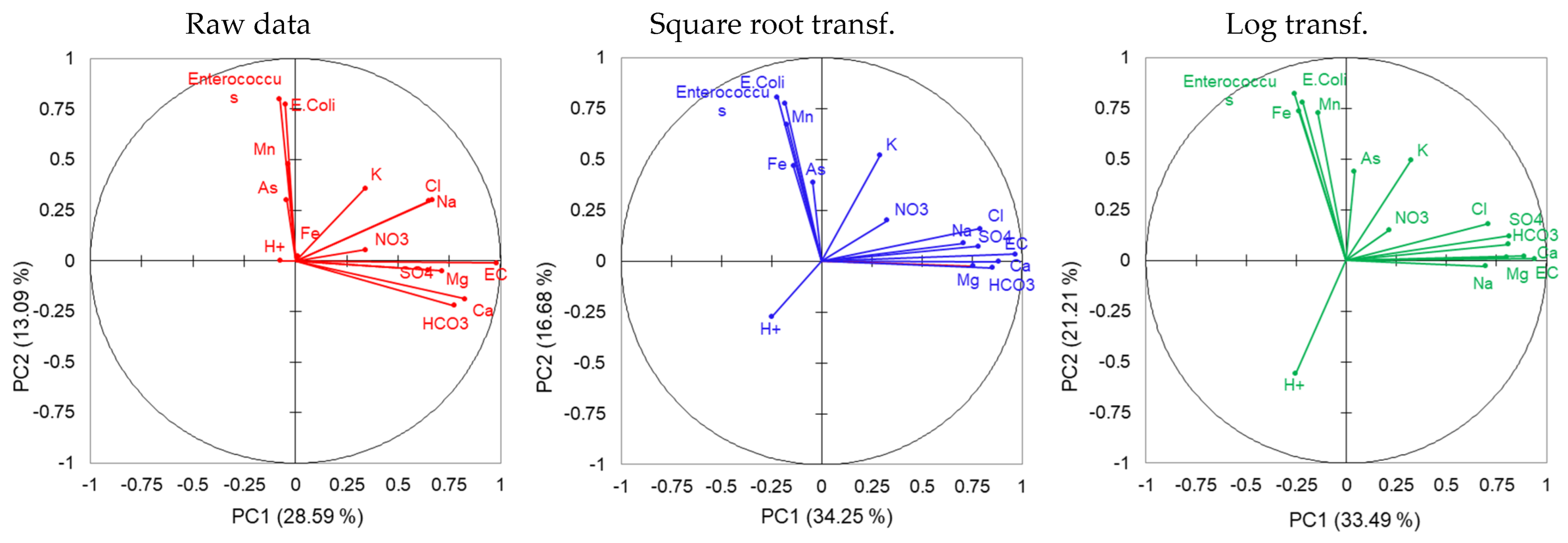
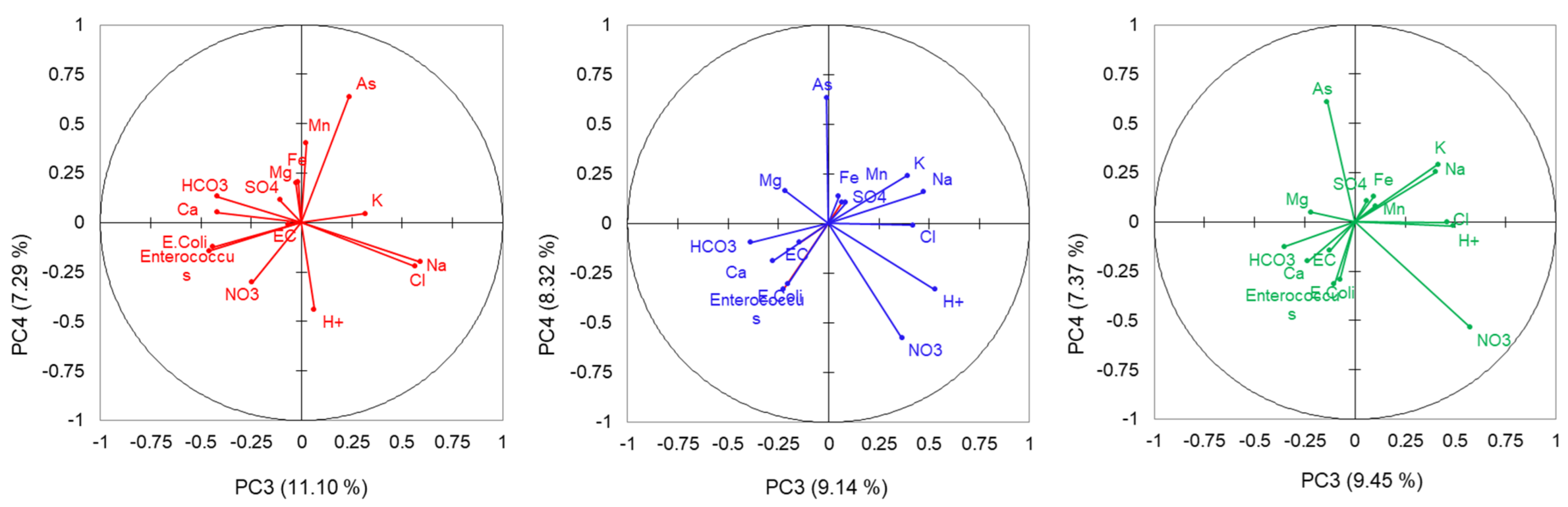
3.3. PCA Using the 3 Data Conditioning Modes

The results of the PCAs conducted with the three different modes of data conditioning are summarized in

Table 2. Variance explained by the main factorial axes (PCs) for 3 data-conditioning mode.

	Raw Data	Explained Variance Square Root Transf.	Log Transf.
PC1	28.59	34.25	33.49
PC2	13.09	16.68	21.21
PC3	11.1	9.14	9.45
PC4	7.29	8.32	7.37
Sum	60.07	68.39	71.52

.

3.3.1. Significance of the First Four Principal Components

Whatever the data conditioning procedure, the significance of the factorial axes was more or less the same, without any major difference (Figure 2): the first factorial axis reflected the water mineral load, with electrical conductivity and major elements on the positive side, and less soluble minor elements on the negative one. The second factorial axis conveyed the fecal bacterial load positively correlated to Fe and Mn metals. For the log conditioning, the pH had a significant effect on this second axis, which is not the case for the analysis with the raw data. The third factorial axis showed an opposition between samples with a Na-Cl chemical profile on the one hand and a Ca-HCO3 profile on the other. Finally, the fourth factorial axis reflected arsenic contents in all cases.

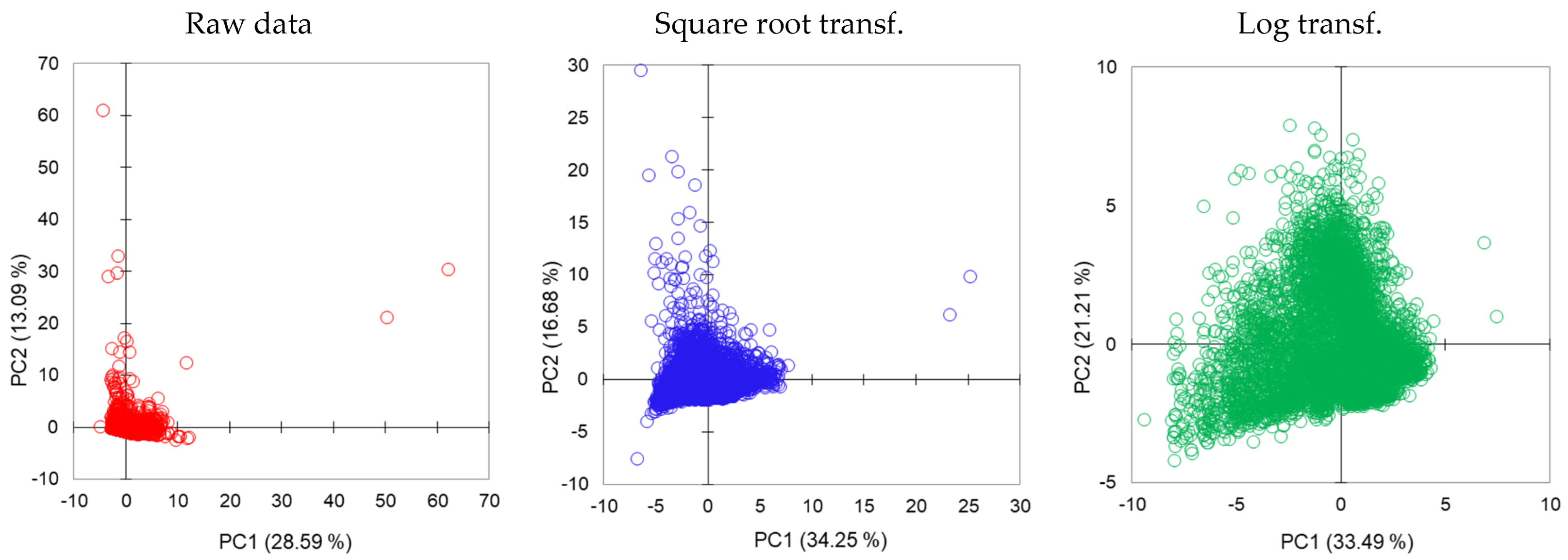
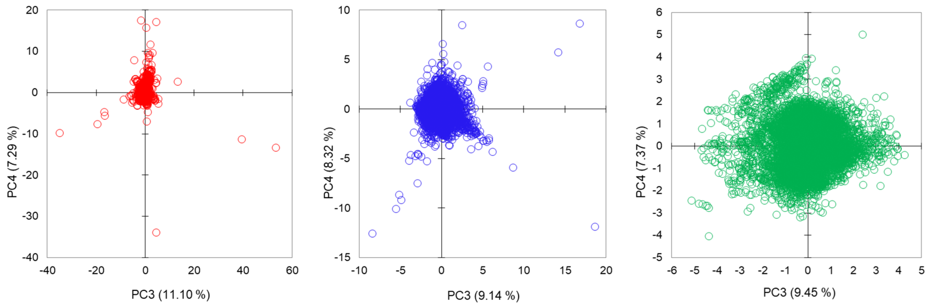
3.3.2. Distribution of Water Samples in Factorial Score Plots

The distribution of samples in the PC1/PC2 and PC3/PC4 factorial plans were plotted for the three modes of data conditioning in Figure 3. The difference in the distribution of the scatterplots was notable. In the case of raw data, a small number of extreme values monopolized most of the information and thus the variance, regardless of the origin of the variability, i.e., dissolved load, bacterial load, or other parameters. It resulted in factorial plans with large areas without observations, bounded only by a few rare points, while almost all the observations of the database (more than 7000) were grouped in a small central area. On the other hand, after the logarithmic transformation or to a lesser extent the square root transformation, the extreme values played a much more moderate role and the observations were spread over the factorial planes, which allowed us to better visualize the diversity of the information contained in the database.

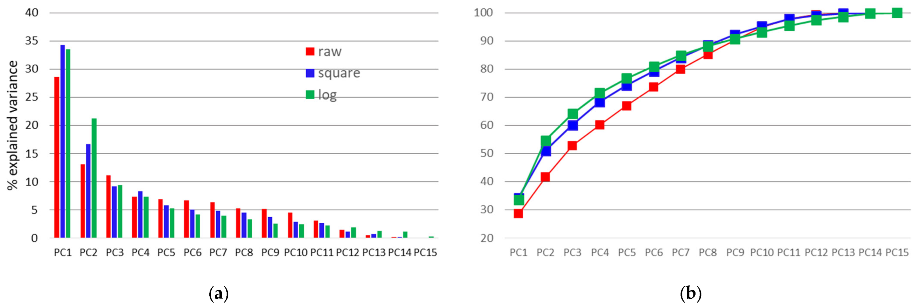
3.3.3. Inertia of the Principal Components

The cumulative inertia of the principal components is presented in

Table 3. Table of variances for PC 1 to PC7 and 3 conditioning modes.

		PC1	PC2	PC3	PC4	PC5	PC6	PC7
Raw data	Eigenvalue	4.29	1.96	1.67	1.09	1.03	1	0.96
	Variability (%)	28.59	13.09	11.10	7.29	6.85	6.65	6.38
	Cumulative %	28.59	41.68	52.78	60.07	66.92	73.58	79.95
Squ. root data	Eigenvalue	5.14	2.50	1.37	1.25	0.87	0.75	0.72
	Variability (%)	34.25	16.68	9.14	8.32	5.83	5.02	4.79
	Cumulative %	34.25	50.94	60.07	68.39	74.22	79.24	84.03
Log. data	Eigenvalue	5.02	3.18	1.42	1.11	0.79	0.62	0.59
	Variability (%)	33.5	21.21	9.45	7.37	5.25	4.16	3.93
	Cumulative %	33.5	54.71	64.16	71.53	76.78	80.93	84.86

up to PC7 and can be compared in Figure 4 for the three modes of data conditioning. With the raw data, we observe that the first PC accounted for only 28% of the variance, while it accounted for 33 and 34% for the log- or Square root-transformed data, respectively. There was thus a significant gap between the different modes of data conditioning. If we consider the four main factorial axes, the gap appeared to be even larger, going from 60% with the raw data to 71.5% with a logarithmic transformation of the data, with the square root transformation giving an intermediate result (68.4%).

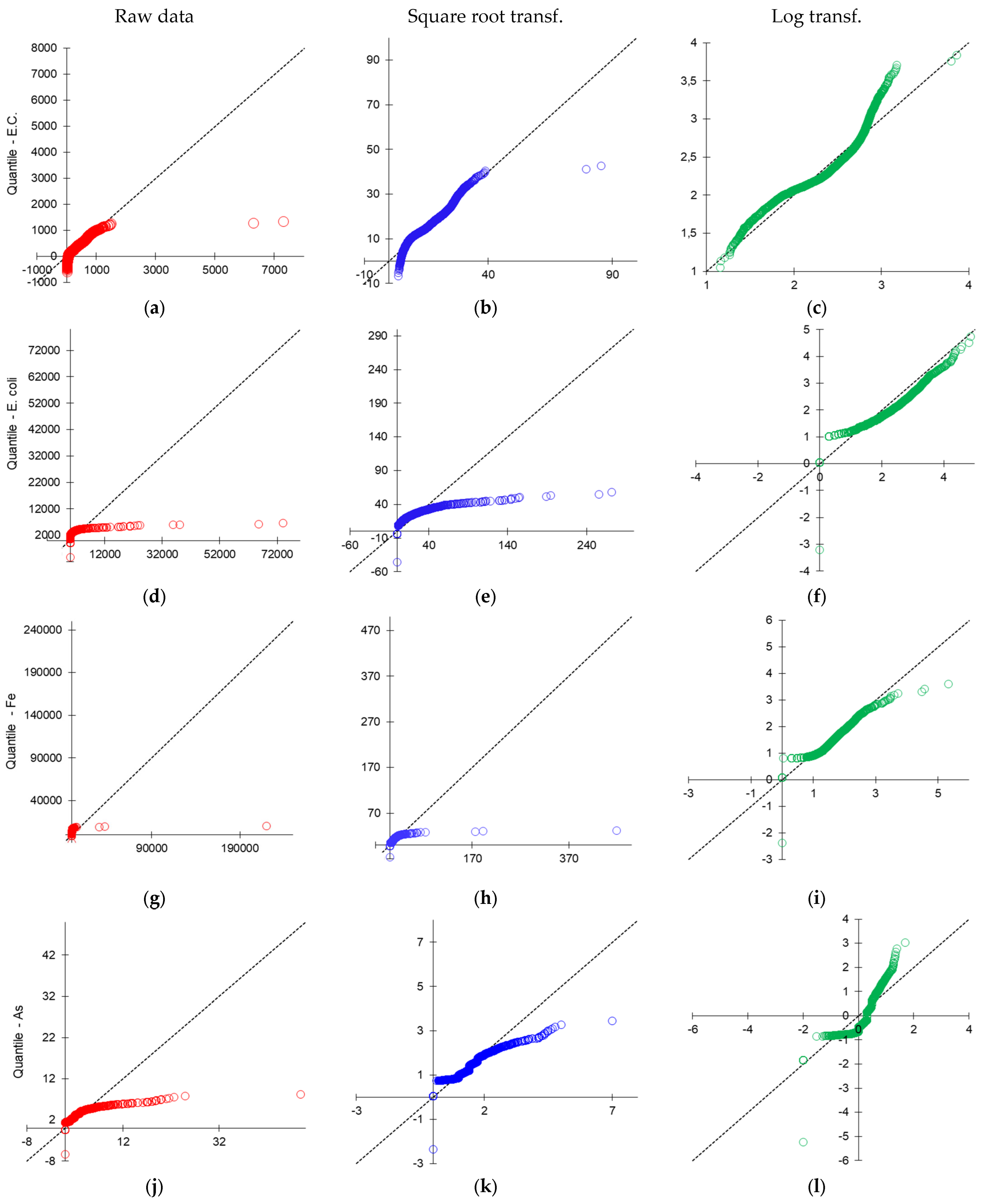
3.4. Frequency Distribution

The Q-Q plots are shown in Figure 5 for some key parameters, namely EC representing mineralization, E. coli, sensitive to bacteriological contamination, Fe sensitive to redox processes and As concentration. The frequency distribution differs somewhat depending on the parameter. For the different bacteriological and physicochemical parameters, the Kolmogorov–Smirnov normality tests indicate a non-normal distribution, which can be visualized on the Q-Qplot (Figure 5). There is an important dissymmetry linked to the existence of some high values. The logarithmic transformation leads to a change in scale, compacting the axes for the extreme values and dilating the axes for the low values. The distribution then approached a normal distribution, although the normality test was still negative for all parameters. The square root transformation also resulted in a similar contraction of the high values and dilation of the low values but gave intermediate results between using the raw data and the log transformation.

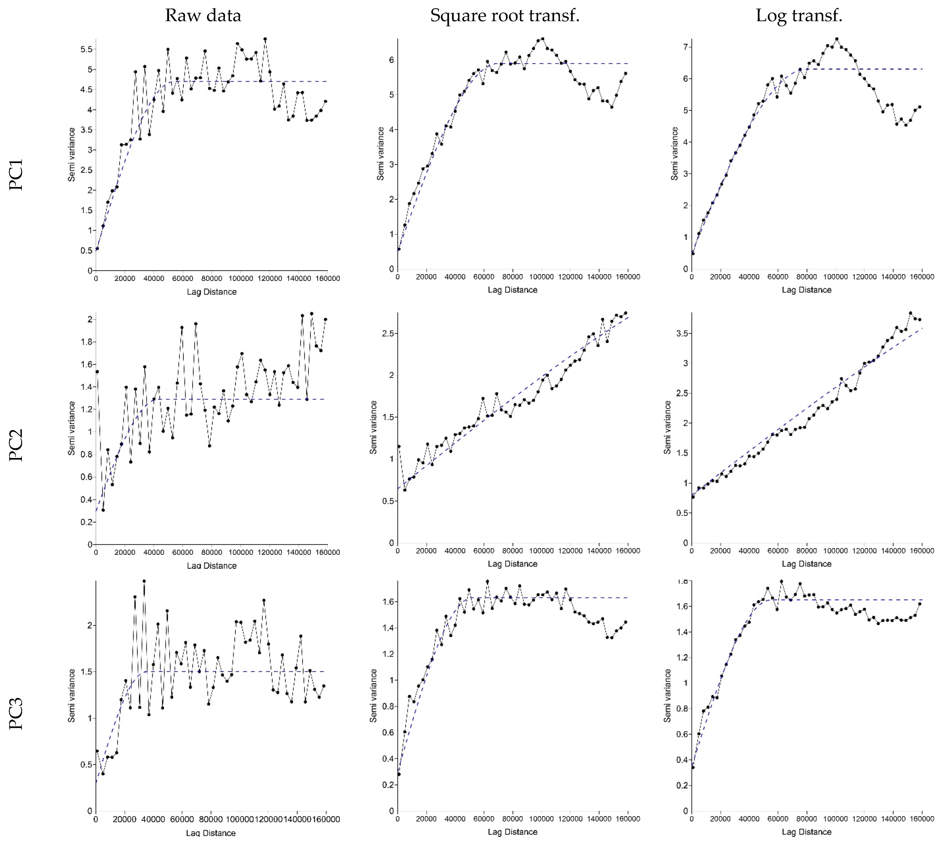
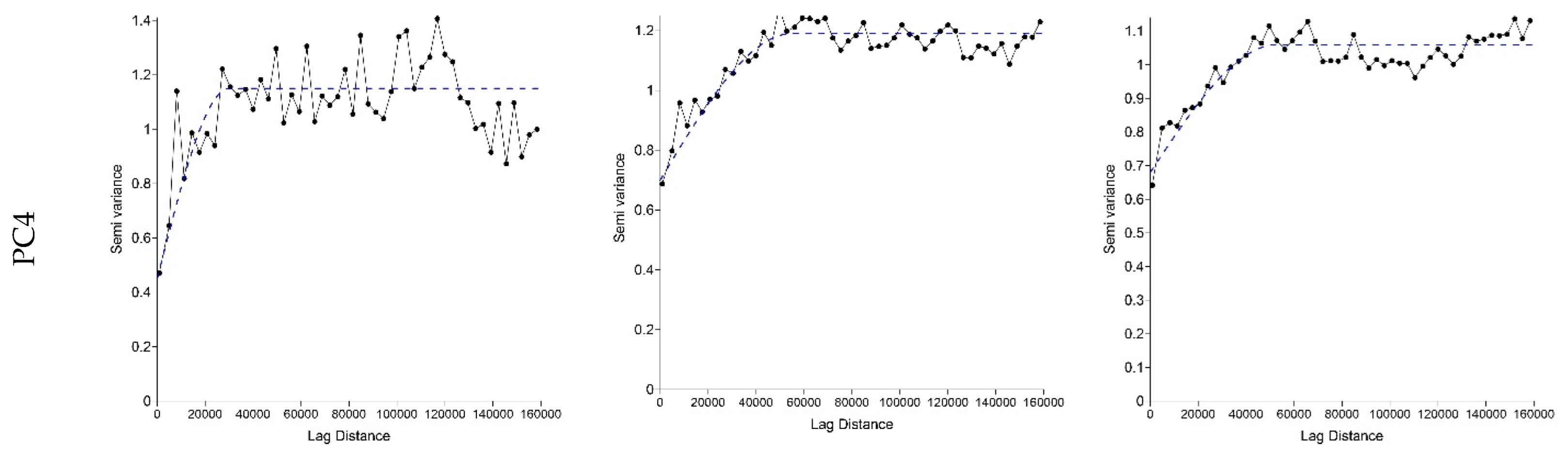
3.5. Variograms and Mapping

The variograms for the macroparameters (PC1 to PC4) and for the three modes of data conditioning are presented in Figure 6. All experimental variograms were fitted by spherical models whose characteristics are summarized in

Table 4. Characteristics of the spherical models fitted on the experimental variograms.

		Raw Data	Square Root Transf.	Log Transf.
PC1	Nugget	0.5	0.5	0.5
	Range	54,000	70,000	80,000
	Reduced sill	4.2	5.4	5.8
PC2	Nugget	0.3	0.75	0.8
	Range	43,000	350,000	300,000
	Reduced sill	1	3.2	4.9
PC3	Nugget	0.3	0.3	0.35
	Range	35,000	52,000	55,000
	Reduced sill	1.2	1.33	1.3
PC4	Nugget	0.45	0.7	0.68
	Range	30,000	55,000	53,000
	Reduced sill	0.7	0.49	0.38

. These fitted models were applied to draw up the distribution maps of the PCs over the entire Occitanie region. Whatever the parameters, the variograms calculated on the log-transformed data showed little irregularity unlike the variograms calculated on the raw data. Again, the square root transformation was intermediate between the raw data and the log-transformed data. The reduced sill/Nugget ratio increased between raw data (8.4 and 3.3), square root transformation (10.8 and 4.3) and Log-transformation (11.6 and 6.1) for PC1 and PC2 respectively, while this was not true for the following PCs.

The mode of data conditioning generated significant differences on the maps obtained by kriging (Figure 7). In particular, when using the raw data, the few extreme values induced large homogeneous color ranges that prevented distinguishing the nuances of local variability, except by arbitrarily modifying the color scales. With the transformation of the data, by logarithm and to a lesser extent by square root, these drawbacks disappeared and the spatial variabilities were revealed, both local and regional.

Differences were not observed for all parameters. For example, for electrical conductivity and major ions, we noted the absence of extreme values. Thus, the distribution maps of PC1 and PC3 mainly influenced by these parameters showed a well-distributed scale between the minimum and maximum values. These two PCs are also characterized by a long range in the variograms due to the influence of lithology. The conditioning of the data only moderately alters the appearance of the maps. This was not the case for bacteriological parameters or minor elements, mainly represented by PC2, nor even for nitrogenous pollution represented by PC4, and for which the extreme values shifted the scale towards the high values, the lowest color range covering most of the area. There is also a much shorter range in these PCs due to the local influence of processes on trace elements or nitrogenous forms. The log transformation allows a better distribution of colors and reveals the local or regional character of the pollution.

4. Discussion

4.1. Need to Work on Transformed Data

The choice of transforming the data before studying the frequency distribution may face different difficulties. One of these is reported by O’Hara and Kotze [34] and concerns the fact that in many cases there are zero values. However, for the concentration of dissolved elements, an element always exists at least in trace amounts, and therefore, the value of zero is very implausible. With zero values, the logarithmic transformation is impossible because log (0) does not exist. To get around this problem, we made two choices when preparing the database: On the one hand, observations with missing values were eliminated from the processed database, and on the other hand, the detection limit replaced the values that were below it. Indeed, some analytical laboratories report a value below the detection limit, and others assign a value of 0, but in reality, the only certainty is that the value is between 0 and the detection limit. Feng et al. [35] mentioned that if the original data follow a log-normal or approximately normal distribution, then the log-transformed data follow a normal or approximately normal distribution and the log transformation removes or reduces the skewness. The data from many studies, however, do not approximate the lognormal distribution and applying this transformation does not reduce the skewness of the distribution. One of the key criteria is skewness, which is related, for example, to the existence of extremely high or extremely low values relative to the mean in a data set. The larger the database (several thousand or tens of thousands of observations), i.e., covering a longer period of time or a larger and heterogeneous region, the more likely it is to contain extreme values, thus generating a skewed distribution. It also appears that the use of PCA without prior data conditioning is not an alternative to data conditioning. Indeed, since the PCs are a linear combination of the original parameters they maintain the problems associated with the presence of extreme values and a highly skewed frequency distribution of the data.

Given this observation, what are the options for ensuring that the information carried by these extreme values does not mask a large part of the information contained in the database? The first phase would, therefore, be a diagnostic phase aiming at identifying whether these extreme values are high or low. In the case of high values, the corresponding observations can be eliminated, resulting in a net loss of information in the database. However, this information, although atypical, is often local, with a high impact on a small number of observations, but probably interesting, and is an integral part of the analyzed database. Another solution is to limit the extreme values, which generally concern only one or two parameters (most often bacteriological parameters or metals) out of a few dozen observations. The loss of information is less. The third option is a data transformation, which must have the following properties. This transformation must be continuous, dilate the gaps between the weak values, and contract those between the strong values in order to make the distribution more symmetrical and thus rebalance the weight of useful information. Several possibilities exist. The first is to apply an inverse function (1/x), which results in reversing the order of the data but is only applicable when the extremes correspond to strong values, without values close to zero. A second option is a transformation by the square root or any other power between 0 and 1. This transformation will have the effect of dilating the weak values and contracting the strong values but may be insufficient, or less efficient than a logarithmic transformation, as we observed on the Occitanie dataset. Note, that for inverse or log transformations there is the problem of undefined null values, a point we discussed above.

4.2. Impact on Process Analysis

The main difference between PCA on raw data and transformed data, and in particular on log-transformed data, is that the effect of extreme values is reduced. The dispersion of the observations is thus distributed in the first score plots of the PCA, making it possible to better represent the significance of the factorial axes, without the interfering effect of a small number of samples. This results in better visualization and efficiency of the analysis, which is measured, on the Occitanie database treated in this work, by the percentage of variance explained by the first four factorial axes, increasing from 60 to 71.5%. With or without transformation of the data, the first score plot PC1-PC2, which carries about half of the information, reflects the same realities (minerality and fecal contamination of the water), the same processes, but in a much more efficient way with log conditioning. Similarly, for the third and fourth PCs, the significance of the axes (chemical profile and nitrogen pollution, respectively) is more or less the same whether the data are in log or not, but the information is more condensed and efficient. As these axes act as macro-parameters, they reflect associated processes that are more clearly defined.

The importance of data conditioning on the percentage of variance explained is in line with that of comparisons on distributions and their deviation from the normal distribution. However, two points should be kept in mind. (1) In the case of data from very different natural environments, as is the case with water quality data acquired on a regional scale, in various geological, climatic and land use contexts, the distribution cannot be truly normal because it is composed of the superposition of distributions of data from different environments, each with its own distribution. For illustration, if we look at the EC parameter in the Occitanie region, the range is between 20 and 50 µS cm⁻¹ for mountainous crystalline basement areas, 250 and 500 µS cm⁻¹ for karst environments, and 800 and 1000 µS cm⁻¹ within coastal plains. In this case, the log transformation can be very useful to simply approximate the set of values to a normal distribution. (2) Although the deviation from a normal distribution is troublesome, the consequences are less severe than for the calculation of principal components. Indeed, in the processing of large databases such as SISE-EAUX [25], dimensional reduction is an essential step for the synthetic mapping of groundwater quality data at the regional scale. It is part of a proven procedure for grouping groundwater bodies that are similarly more or less vulnerable to contamination via similar mechanisms [29]. The more information the main factorial axes convey, the more efficient the dimensional reduction, and the better the clustering of groundwater body families and consequently the analysis of the mechanisms responsible for the variability of the chemical composition of the water within each groundwater body family. Log transformation of data is, therefore, necessary for large databases that are likely to have extreme values, not for approximation to a normal distribution, but for a better dimensional reduction in the data hyperspace and clustering of groundwater bodies, which will facilitate analysis of the processes responsible for quality variability. The advances of this study carried out on Occitanie are currently being introduced in other French administrative regions (Provence-Alpes-Côte d’Azur, Bourgogne-Franche Comté, Auvergne-Rhône-Alpes, etc.) as well as in the territory of Corsica. Taking into account the extreme values in the databases, but attenuating their weight, allows a better vision of the spatial and temporal variability, leading to a better grouping of groundwater bodies intended for human consumption. Quality monitoring and surveillance by health agencies can thus be optimized, resulting in lower costs. Subject to the existence of similar databases in other European countries, the procedure could be applied there.

Although correlation is not proof of causality, the multiple correlations illustrate that the way in which the data are conditioned can reveal a correlation between fecal contamination and all the other parameters. The calculation of the R² (Table 1) quantifies this correlation and illustrates that Log conditioning is the most efficient. The square root conditioning reveals this correlation, but compared to the Log conditioning, it explains only half of the variance (26% vs. 49%). Such a proportion in the explained variance highlights that the extreme values monopolize a large part of the useful information conveyed by the factorial axes, masking the influence of the bulk of the database, which is revealed by the Log transformation. We also notice that the few samples with extreme values do not follow the same correlations between parameters as the majority of the other observations in the database. Indeed, if these correlations had been similar, the logarithmic or square root transformation would decrease their coordinates on the principal components, but would not change the percentage of variance explained. The increase in explained variance, therefore, reflects a reduction in statistical background noise [30] and an improvement in the definition of principal components for the majority of observations. We can also note an effect on the mapping of the main PCs. If the reduced sill/Nugget ratio increases between the raw data, square root and log transformation, this reflects that the essential and structured information is concentrated on the first factorial axes. In other words, with the log transformation, useful and spatially well-structured information is concentrated in the first axes while unstructured variability is redistributed to the following PCs. With the raw data, the unhelpful and spatially ill-structured information already contaminates the first factorial axes. Thus, the information contained in the extracted database is better structured in terms of variance distribution but also in terms of spatial distribution after log transformation rather than using the raw data without conditioning.

5. Conclusions

In large-dimension multiparametric databases on the quality of water intended for human consumption, the risk of the appearance of extreme values is high, especially for metals and bacteriological parameters. A few water analyses concentrate most of the information, which disturbs the study of the rest of the information. To this effect, the Log transformation appears to be the best option allowing (1) to reduce, without eliminating or limiting them, the influence of extreme values which otherwise have an important impact on the global variance, even if they are few in number; (2) to highlight certain correlations between bacteriological and physicochemical parameters; (3) to significantly increase the readability of the factorial axes as well as the identification and the cartographic representation of the associated processes responsible for the variance within the database. Taking these results into account will improve the grouping of groundwater bodies according to physicochemical and bacteriological water characteristics, an aspect that will be addressed in future work for the Occitanie region, but also at other scales throughout the Rhone basin.

References

1. International Association of Hydrogeologists. Groundwater—More About the Hidden Resource. Available online: https://iah.org/education/general-public/groundwater-hidden-resource (accessed on 27 November 2022).
2. Li, P. To Make the Water Safer. Expo. Health 2020, 12, 337–342. [Google Scholar] [CrossRef] [PubMed]
3. European Commission. Directive 2000/60/EC of the European Parliament and of the Council of 23 October 2000 establishing a framework for Community action in the field of water policy. Off. J. Eur. Communities 2000, 22, 2000. [Google Scholar]
4. European Commission. Directive 2006/118/EC of the European Parliament and of the Council of 12 December 2006 on the protection of groundwater against pollution and deterioration. Off. J. Eur. Union 2006, 372, 19–31. [Google Scholar]
5. Martínez Navarrete, C.; Grima Olmedo, J.; Durán Valsero, J.J.; Gómez Gómez, J.D.; Luque Espinar, J.A.; de la Orden Gómez, J.A. Groundwater protection in Mediterranean countries after the European water framework directive. Environ. Geol. 2008, 54, 537–549. [Google Scholar] [CrossRef]
6. Danielopol, D.L.; Griebler, C.; Gunatilaka, A.; Notenboom, J. Present state and future prospects for groundwater ecosystems. Environ. Conserv. 2003, 30, 104–130. [Google Scholar] [CrossRef] [Green Version]
7. Edmunds, W.M.; Shand, P.; Hart, P.; Ward, R.S. The natural (baseline) quality of groundwater: A UK pilot study. Sci. Total Environ. 2003, 310, 25–35. [Google Scholar] [CrossRef] [Green Version]
8. Hinsby, K.; Condesso de Melo, M.T.; Dahl, M. European case studies supporting the derivation of natural background levels and groundwater threshold values for the protection of dependent ecosystems and human health. Sci. Total Environ. 2008, 401, 1–20. [Google Scholar] [CrossRef]
9. Masciale, R.; Amalfitano, S.; Frollini, E.; Ghergo, S.; Melita, M.; Parrone, D.; Preziosi, E.; Vurro, M.; Zoppini, A.; Passarella, G. Assessing Natural Background Levels in the Groundwater Bodies of the Apulia Region (Southern Italy). Water 2021, 13, 958. [Google Scholar] [CrossRef]
10. Nakić, Z.; Kovač, Z.; Parlov, J.; Perković, D. Ambient Background Values of Selected Chemical Substances in Four Groundwater Bodies in the Pannonian Region of Croatia. Water 2020, 12, 2671. [Google Scholar] [CrossRef]
11. Quevauviller, P.; Balabanis, P.; Fragakis, C.; Weydert, M.; Oliver, M.; Kaschl, A.; Arnold, G.; Kroll, A.; Galbiati, L.; Zaldivar, J.M.; et al. Science-policy integration needs in support of the implementation of the EU Water Framework Directive. Environ. Sci. Policy 2005, 8, 203–211. [Google Scholar] [CrossRef]
12. Smith, J.W.N.; Bonell, M.; Gibert, J.; McDowell, W.H.; Sudicky, E.A.; Turner, J.V.; Harris, R.C. Groundwater–surface water interactions, nutrient fluxes and ecological response in river corridors: Translating science into effective environmental management. Hydrol. Process. 2008, 22, 151–157. [Google Scholar] [CrossRef]
13. Urresti-Estala, B.; Carrasco-Cantos, F.; Vadillo-Pérez, I.; Jiménez-Gavilán, P. Determination of background levels on water quality of groundwater bodies: A methodological proposal applied to a Mediterranean River basin (Guadalhorce River, Málaga, southern Spain). J. Environ. Manag. 2013, 117, 121–130. [Google Scholar] [CrossRef] [PubMed]
14. Wendland, F.; Hannappel, S.; Kunkel, R.; Schenk, R.; Voigt, H.J.; Wolter, R. A procedure to define natural groundwater conditions of groundwater bodies in Germany. Water Sci. Technol. 2005, 51, 249–257. [Google Scholar] [CrossRef] [PubMed]
15. John, D.E.; Rose, J.B. Review of Factors Affecting Microbial Survival in Groundwater. Environ. Sci. Technol. 2005, 39, 7345–7356. [Google Scholar] [CrossRef] [PubMed] [Green Version]
16. Pachepsky, Y.A.; Shelton, D.R. Escherichia coli and Fecal Coliforms in Freshwater and Estuarine Sediments. Crit. Rev. Environ. Sci. Technol. 2011, 41, 1067–1110. [Google Scholar] [CrossRef]
17. Pandey, P.K.; Kass, P.H.; Soupir, M.L.; Biswas, S.; Singh, V.P. Contamination of water resources by pathogenic bacteria. AMB Express 2014, 4, 51. [Google Scholar] [CrossRef] [Green Version]
18. Haslauer, C.P.; Heißerer, T.; Bárdossy, A. Including land use information for the spatial estimation of groundwater quality parameters—2. Interpolation methods, results, and comparison. J. Hydrol. 2016, 535, 699–709. [Google Scholar] [CrossRef]
19. Haslauer, C.P.; Allmendinger, M.; Gnann, S.; Heisserer, T.; Bárdossy, A. Interpolation of Regional Groundwater Quality Parameters With Categorical and Real-Valued Secondary Information in the State of Baden-Württemberg, Germany. In Proceedings of the AGU Fall Meeting Abstracts, New Orleans, LA, USA, 11–15 December 2017; Volume 2017, p. H53O-07. [Google Scholar]
20. Frollini, E.; Preziosi, E.; Calace, N.; Guerra, M.; Guyennon, N.; Marcaccio, M.; Menichetti, S.; Romano, E.; Ghergo, S. Groundwater quality trend and trend reversal assessment in the European Water Framework Directive context: An example with nitrates in Italy. Environ. Sci. Pollut. Res. 2021, 28, 22092–22104. [Google Scholar] [CrossRef]
21. Pantaleone, D.V.; Vincenzo, A.; Fulvio, C.; Silvia, F.; Cesaria, M.; Giuseppina, M.; Ilaria, M.; Vincenzo, P.; Rosa, S.A.; Gianpietro, S.; et al. Hydrogeology of continental southern Italy. J. Maps 2018, 14, 230–241. [Google Scholar] [CrossRef] [Green Version]
22. El Osta, M.; Masoud, M.; Alqarawy, A.; Elsayed, S.; Gad, M. Groundwater Suitability for Drinking and Irrigation Using Water Quality Indices and Multivariate Modeling in Makkah Al-Mukarramah Province, Saudi Arabia. Water 2022, 14, 483. [Google Scholar] [CrossRef]
23. Masoud, M.; El Osta, M.; Alqarawy, A.; Elsayed, S.; Gad, M. Evaluation of groundwater quality for agricultural under different conditions using water quality indices, partial least squares regression models, and GIS approaches. Appl. Water Sci. 2022, 12, 244. [Google Scholar] [CrossRef]
24. Webster, R.; Olliver, M.A. Geostatistics for Environmental Scientists, 2nd ed.; Wiley: Chichester, UK, 2007; ISBN 9780470028582. [Google Scholar]
25. Tiouiouine, A.; Yameogo, S.; Valles, V.; Barbiero, L.; Dassonville, F.; Moulin, M.; Bouramtane, T.; Bahaj, T.; Morarech, M.; Kacimi, I. Dimension reduction and analysis of a 10-year physicochemical and biological water database applied to water resources intended for human consumption in the provence-alpes-cote d’azur region, France. Water 2020, 12, 525. [Google Scholar] [CrossRef]
26. Barbel-Périneau, A.; Barbiero, L.; Danquigny, C.; Emblanch, C.; Mazzilli, N.; Babic, M.; Simler, R.; Valles, V. Karst flow processes explored through analysis of long-term unsaturated-zone discharge hydrochemistry: A 10-year study in Rustrel, France. Hydrogeol. J. 2019, 27, 1711–1723. [Google Scholar] [CrossRef]
27. Helena, B.; Pardo, R.; Vega, M.; Barrado, E.; Fernandez, J.M.; Fernandez, L. Temporal evolution of groundwater composition in an alluvial aquifer (Pisuerga River, Spain) by principal component analysis. Water Res. 2000, 34, 807–816. [Google Scholar] [CrossRef]
28. Rezende Filho, A.T.; Furian, S.; Victoria, R.L.; Mascré, C.; Valles, V.; Barbiero, L. Hydrochemical variability at the upper paraguay basin and pantanal wetland. Hydrol. Earth Syst. Sci. 2012, 16, 2723–2737. [Google Scholar] [CrossRef] [Green Version]
29. Tiouiouine, A.; Jabrane, M.; Kacimi, I.; Morarech, M.; Bouramtane, T.; Bahaj, T.; Yameogo, S.; Rezende-Filho, A.; Dassonville, F.; Moulin, M.; et al. Determining the relevant scale to analyze the quality of regional groundwater resources while combining groundwater bodies, physicochemical and biological databases in southeastern france. Water 2020, 12, 3476. [Google Scholar] [CrossRef]
30. Rezende Filho, A.; Valles, V.; Furian, S.; Oliveira, C.M.S.C.; Ouardi, J.; Barbiero, L. Impacts of lithological and anthropogenic factors affecting water chemistry in the Upper Paraguay River Basin. J. Environ. Qual. 2015, 44, 1832–1842. [Google Scholar] [CrossRef]
31. Marden, J.I. Positions and QQ Plots. Stat. Sci. 2004, 19, 606–614. [Google Scholar] [CrossRef]
32. Steinskog, D.J.; Tjøstheim, D.B.; Kvamstø, N.G. A Cautionary Note on the Use of the Kolmogorov–Smirnov Test for Normality. Mon. Weather Rev. 2007, 135, 1151–1157. [Google Scholar] [CrossRef]
33. Bouramtane, T.; Yameogo, S.; Touzani, M.; Tiouiouine, A.; El Janati, M.; Ouardi, J.; Kacimi, I.; Valles, V.; Barbiero, L. Statistical approach of factors controlling drainage network patterns in arid areas. Application to the Eastern Anti Atlas (Morocco). J. African Earth Sci. 2020, 162, 103707. [Google Scholar] [CrossRef]
34. O’Hara, R.B.; Kotze, D.J. Do not log-transform count data. Methods Ecol. Evol. 2010, 1, 118–122. [Google Scholar] [CrossRef] [Green Version]
35. Feng, C.; Wang, H.; Lu, N.; Chen, T.; He, H.; Lu, Y.; Tu, X.M. Log-transformation and its implications for data analysis. Shanghai Arch. Psychiatry 2014, 26, 105–109. [Google Scholar] [PubMed]
Figure 1. Location of the Occitanie region in southern France. Elevation and groundwater sampling points and major subregions.
Water 15 00084 g001
Figure 2. Distribution of the variables in the main factorial plans.
Water 15 00084 g002aWater 15 00084 g002b
Figure 3. Distribution of the observation in the factorial plans PC1-PC2 and PC3-PC4 for raw data, square root transformation and log transformation.
Water 15 00084 g003aWater 15 00084 g003b
Figure 4. Variance (a) and cumulative variance (b) explained by the principal components using raw data, square root and logarithm transformation.
Water 15 00084 g004
Figure 5. Quantile-quantile plots for Electrical Conductivity (ac), E. coli (d–f), Fe (gi) and As (jl) for raw, square root- and log-transformed data.
Water 15 00084 g005
Figure 6. Experimental variograms and fitted spherical models for PC1 to PC4 (distance in m).
Water 15 00084 g006aWater 15 00084 g006b
Figure 7. Distribution of the first four factorial axes over the Occitanie region using raw data, square root transformation and log transformation of the data.
Water 15 00084 g007aWater 15 00084 g007b