Fast Recognition on Shallow Groundwater and Anomaly Analysis Using Frequency Selection Sounding Method

Abstract

The validity of the frequency selection method (FSM) in shallow (<150 m) groundwater exploration was illustrated by practical applications, and the relationship between potential electrode spacing MN and groundwater depth in FSM sounding method was analyzed and preliminary theoretical research was carried out by a simple geologic-geophysical model of sphere. Firstly, under the combined action of horizontal alternating electric field and alternating magnetic field, a simplified geophysical model of low resistivity conductive sphere in homogeneous half space was established, and the forward calculation was performed on the FSM sounding curve. Then, the water yield of 131 wells in the application of FSM in the Rural Drinking Water Safety Project of 12th Five-Year Plan in Guangxi Province was counted. In addition, detailed tabular statistical analysis was carried out on the drilling results of 98 drilling wells, and the relationship between potential electrode spacing MN at abnormal sounding curve and actual drilling water depth was compared and studied. Theoretical analysis and practical application show that FSM has obvious effectiveness in shallow groundwater exploration, and it is an effective method to determine shallow groundwater well locations in the future. The cause of FSM anomaly is the comprehensive effect of the natural 3D alternating electromagnetic signal underground. At the same time, the practical statistics show that there is 1:1 approximation between the size of potential electrode spacing MN at the anomaly curve of the frequency selection method and the actual drilling water depth, which verifies the correctness of the theoretical simulation results. FSM could be widely used in the shallow groundwater exploration in the future, and it is an effective, non-destructive, fast, and low-cost geophysical method.

1. Introduction

The frequency selection method of telluric electricity field is simply called the frequency selection method (FSM), which is a passive source electromagnetic exploration method. It is based on the difference of electrical conductivity between underground rocks (ores) and rocks, using magnetotelluric field as the source of the working field. By measuring and studying the variation law of the horizontal component of electric field produced by several natural alternating electromagnetic fields with different frequencies on the ground, the electrical properties of underground geoelectric sections are studied. This method was proposed by Chinese scholars [1]. Since the early 1980s, Chinese scholars have put forward the stray current method (or the audio geoelectric potential method), the acoustic geoelectric field method, the low-frequency geoelectric field method, the frequency selection method of natural electric field, the telluric electrical-field frequency selecting method, the audio frequency telluric electric field method, the natural alternating electric field method, the interfering electric field method, the underground magneto fluid detection method, and so on [1,2,3,4,5,6,7,8,9]. However, the principle and characteristics of the instruments developed or used by the above-mentioned methods are essentially similar to one another. Therefore, the authors hereby call them FSM in this paper. Up to now, scholars have paid much attention to the practical application of this method, especially in the development of instruments and the application of this method in the exploration of groundwater resources and groundwater disasters [10,11,12,13,14,15,16,17], but there is little theoretical research on this method.

FSM is similar to the audio magnetotelluric method (AMT), but it only measures the horizontal electric component of the ground and does not measure the magnetic field component. The frequency selection of this method is mostly at 15 Hz~1.5 kHz, and the potential electrodes spacing of MN is usually 20 m or 10 m when profiling method is used. Therefore, it is an efficient, cost-effective tool for groundwater exploration, and more adaptable than other geophysical prospecting methods in mountainous areas and towns with dense building facilities.

At the same time, FSM is similar to the telluric current prospecting and telluric-telluric profiling (TTP) method, which only measures the electric field component [18,19,20,21,22]. However, telluric current prospecting is suited primarily to sedimentary structures associated with lateral changes in electrical resistivity that are frequently encountered in petroleum and geothermal exploration. The TTP method is an effective and economical geophysical method for detecting the fluctuation of high resistivity bedrock strata, with its frequency 0.01~0.1 Hz and potential electrodes spacing 1~n km. The TTP method is derived from the magnetotellurics (MT) method, and in general, a fixed reference point is chosen in application, and it is often used in conjunction with MT method to calculate the false apparent resistivity, and the work frequency is also different with FSM [18].

According to the previous research results, the source of natural field method is very complex and there are three viewpoints for the field source problem of FSM. The first is that its field source is exactly the same as MT, mainly from the outside of the earth, which is also the view of most scholars. The second is the electromagnetic waves radiated upward from the mantle asthenosphere and the geomagnetic field below the Earth’s interior [2]. The third is that the field source is the industrial stray current field [1].

In recent years, the author has carried out a preliminary study on the causes of profile anomalies in FSM through practical applications and theoretical research [23,24,25,26,27,28,29,30]. The author considers that it is unnecessary to pay special attention to whether the field source of FSM is from the outside of the earth, the inside of the earth or the industrial stray current field. Past successful examples indicate a shallow prospecting depth of FSM in groundwater exploration (generally < 200 m), and anthropogenic electromagnetic noise, such as high-voltage lines and substation equipment, will be avoided as far as possible in practice. According to the controlled source audio-frequency magnetotellurics (CSAMT), it can be approximately considered as the far zone when the separation between receiver and transmitter is greater than three times the skin depth (depth of penetration, investigation depth) [31,32,33,34,35]. The anthropogenic noise has generally been avoided in FSM applications, and the alternating electromagnetic field caused by surface anthropogenic noise can be considered as a far field source. Therefore, the author considers that the field source of FSM can be considered as the comprehensive effect of aforementioned three sources and other electromagnetic field sources that are not recognized. Because all these sources can be considered as far field sources, the primary field source can be simplified to the interaction of horizontal electric field and horizontal magnetic field components in Cartesian coordinate system. Based on this, the author has carried out forward simulation research in the past and obtained the anomalous curve of FSM profiles similar to the measured results [28]. Groundwater is considered as the preferred source of water for meeting domestic, industrial and agricultural requirements, its exploration, rational development and utilization are the issues of great concern to all of us [36,37,38,39,40,41,42,43,44,45]. Since the 1980s, FSM has been gradually widely used and developed in groundwater resources exploration, and instruments have also been gradually improved and automated. For example, the TC series frequency selector manufactured by Hunan Puqi Geological Exploration Equipment Research Institute of Changsha, Hunan, China has now been exported to more than 77 countries in the word and has attained satisfactory results, the technology of this method has been widely recognized by scholars; and the project “Research and Application of Key Technologies for Groundwater Exploration Based on FSM” jointly undertaken by Hunan University of Science and Technology and Hunan Puqi Geological Exploration Equipment Research Institute was awarded the second prize of Hunan Science and Technology Progress Award in 2018. However, a few scholars in China still have doubts about this method, and some even consider it a pseudoscience.

In this paper, the author takes the application of FSM in 12th Five-Year Plan “the rural drinking water safety project” in Guangxi Province as an example and demonstrates the effectiveness of FSM in shallow groundwater exploration from the practical results of 131 boreholes and theoretical research. At the same time, the objective of this paper is to highlight that the anomaly of FSM sounding is related to the potential electrodes spacing. This is in contradiction with the current theory of the magnetotelluric method. It is well known that depth of investigation of the MT method or AMT method is not related to the receiver electric field dipole size. Rather, it is dependent on frequency and resistivity, but not on geometry. This shows that FSM is worthy of further study.

2. Description of the Study Area

2.1. Physical Environment

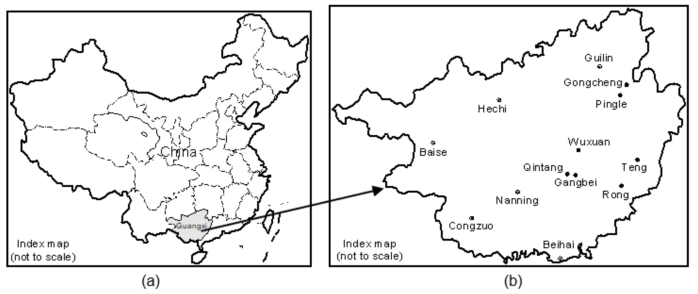
Guangxi Province is located in the southern of China. The area encompasses a total area of about 23.76 × 10⁴ km², and it extends between latitude 20°54′ and 26°24′ N and longitude 104°28′ and 112°04′ E, as shown in Figure 1. Guangxi is located in the southeastern edge of the Yunnan-Guizhou plateau, the second step of China’s terrain. It is located in the western part of the hills of Guangxi and Guangdong provinces and faces the Beibu Gulf in the south. The terrain in this province is high in northwest and low in southeast, inclining from northwest to southeast, and the whole area is geomorphology of mountainous and hilly basins. Because of the compression of the Pacific plate and the Indian Ocean plate, the mountains are mostly arced, and the highest peak in the area is 2141 m above mean sea level (a.m.s.l.). It belongs to the subtropical monsoon climate area, with the average yearly temperature of 17.5~23.5 °C and the average annual rainfall of 841.2~3387.5 mm throughout the province, and the rainy season is concentrated in May~September.

2.2. Geological Environment

Geotectonically, the Guangxi area belongs to the South-China Platform, which was strongly activated in Mesozoic era. The pre-Sinian shallow metamorphic rocks constitute the basement of the platform. According to the difference of geological development history in this area, it can be divided into three units. The northern area is the southern end of the Jiangnan paleocontinent exposed by large basement rock series. The eastern area is mainly the Lower Carboniferous sedimentary caprock, which belongs to a part of the Xiangxi Depression. However, in the vast area, it belongs to Guangxi depression area of the Middle Carboniferous to Triassic sedimentary caprock distribution.

The strata in Guangxi are quite well developed, with Paleozoic sediments as the main deposits, and their depositional development is controlled by Cathaysian tectonic system. The pre-Devonian rock series is composed of clastic sandy shale, schist, phyllite, etc., which distribute in the paleocontinental uplift area and its marginal zone. From Devonian to Triassic, the thick carbonate rocks were mainly accumulated and most widely exposed because of Caledonian movement. Devonian strata can be divided into two groups according to their lithological characteristics, the lower part is quartz sandstone and shale conglomerate, the upper part is mainly gray-white pure limestone, sandy shale and siliceous layer are sandwiched in the middle. The Carboniferous-Permian strata are mainly distributed in the south of the Jiangnan paleocontinent, and the lithofacies differentiation is remarkable, especially in the Permian strata. The bottom of Lower Carboniferous is grey and grey-black layered limestone, and the upper part is coal-measure with varying thickness and drastic changes. The Middle and Upper Carboniferous is mainly composed of gray and gray-white thick-bedded limestone with stable lithofacies. The Lower Permian is black and dark grey limestone, while the upper-Permian is not widely exposed, and its lithofacies changes at the bottom are similar to those described above. The western part of Guangxi accumulated huge thick clastic sandy shale facies during the Triassic period, and there is a thin limestone layer at the bottom. Tertiary strata are developed in eroded valleys, with red calcareous conglomerate and sandstone beds in the lower part and lacustrine sandy shale beds in the upper part. Quaternary strata are not widely distributed in this area, but mainly alluvium, usually with a thickness of only tens of meters.

In addition to aforementioned sedimentary rocks, there are also pre-Sinian granites, Caledonian gneissic granites and Yanshanian granites in the northeastern and southern of Guangxi, of which Yanshanian granites are dominant.

The tectonics of Guangxi is mainly controlled by the mountain-shaped tectonics, the EW tectonics and the Neocathaysian tectonic system. Groundwater in this area can be divided into karstic water and fissure and pore water in sandy shale. Generally speaking, the underground runoff is very good. The former circulates through limestone cave fissures and underground rivers, and it belongs to bicarbonate water. The latter circulates in the fissures and pores of sand shale, mainly in sulfate bicarbonate water. Groundwater is recharged by atmospheric precipitation and discharged by rivers.

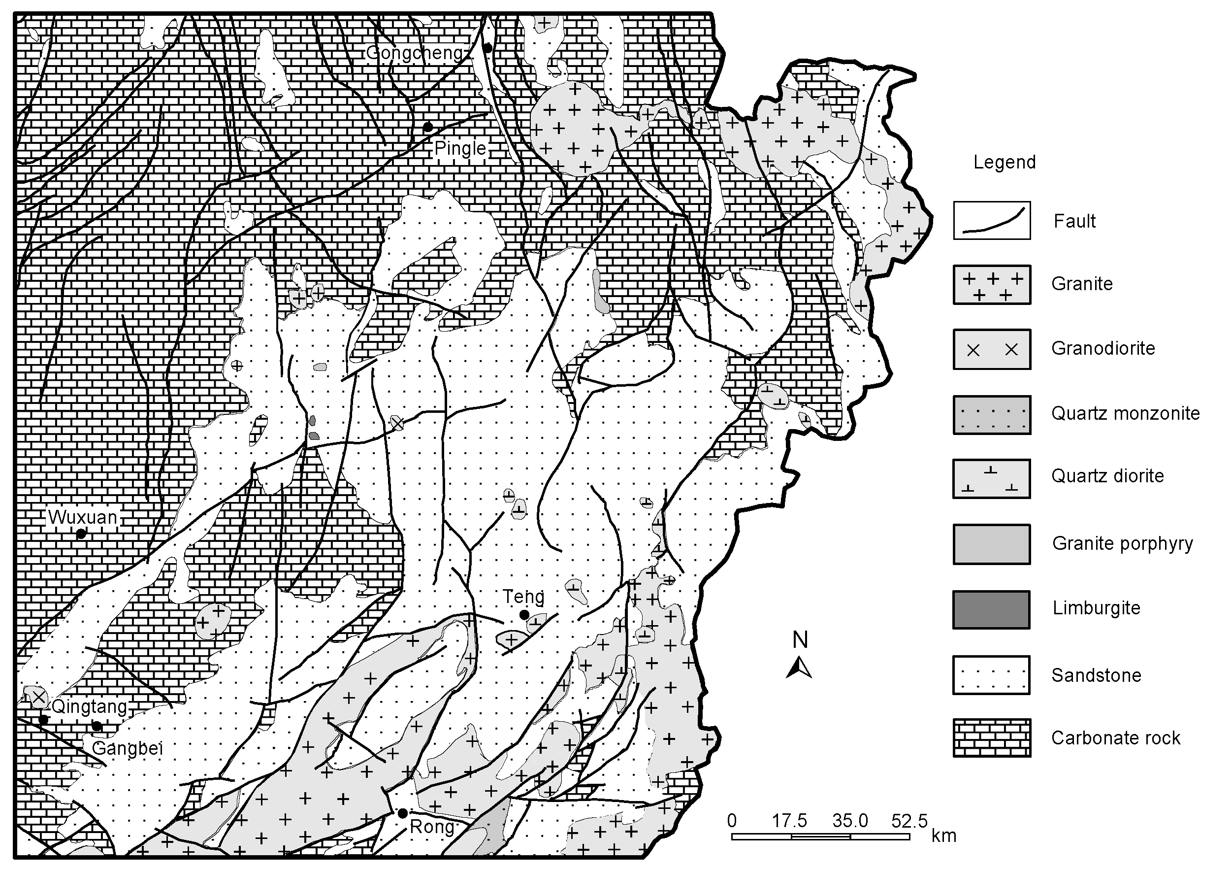
Guangxi Province is recognized as one of the most typical and main karst areas in the world, and the area of karst area is about 9.58 × 10⁴ km², accounting for 40.9% of the total area. The underground fractured karst cave system causes the surface water to leak rapidly and massively into the underground, resulting in water shortage on the ground, which makes it very difficult to use water in Guangxi karst area. The specific location of the application of FSM is located in seven counties of central and eastern Guangxi, such as Wuxuan County, Gongcheng County, Pingle County, Teng County, Rong County, Qingtang District, and Gangbei District, as shown in Figure 1. The regional geology of the area is shown in Figure 2.

3. Methodology

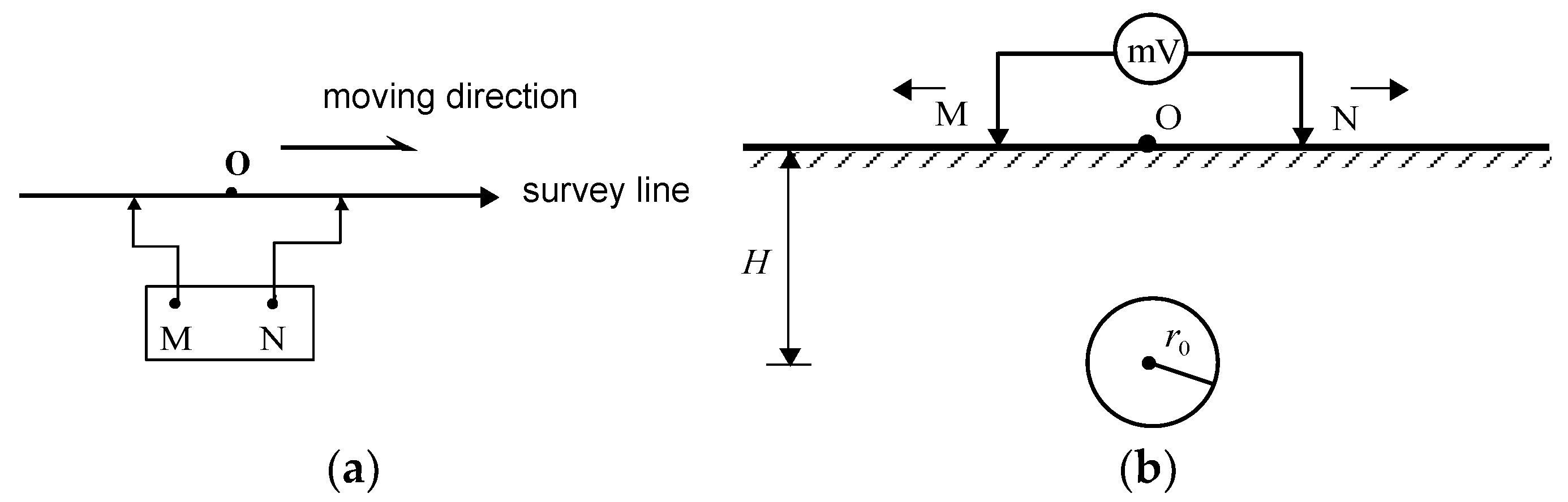
The approach adopted is similar to conventional resistivity profile exploration. The profile detection device of FSM generally adopts parallel movement mode in field measurement, i.e., the potential electrodes M and N move along the survey line with a fixed electrode spacing, and the midpoint O of the measuring electrode spacing MN is a recording point, as shown in Figure 3a. The field electrode spacing MN is usually 10 m or 20 m. The magnitudes of horizontal electric field component ΔV on the surface produced by several different fixed frequency natural electromagnetic fields will be measured at each measuring point. The station spacing is usually 5 m, 10 m, or 20 m, while the station spacing of 1 m or 2 m is used to determine the borehole location. Figure 4a is the profiling detection results of FSM on a survey line in Chetian village, Limu town, Gongcheng County, Guangxi Province, with operating frequencies of 25 Hz, 67 Hz, and 170 Hz. The horizontal axis represents the measuring point, and the vertical axis represents the potential difference in Figure 4a. Because groundwater is generally a relatively good conductor, the place where the relative low potential appears in the profile curve of FSM is the abnormal point, i.e., points of 6, 10, and 13 in Figure 4a are the abnormal points, which can be considered and recommended for the borehole location of groundwater.

The sounding configuration of FSM is similar to the Schlumberger configuration of the conventional vertical electrical sounding method. The measured point lies at O, as shown in Figure 3b, and potential electrodes M and N move outwards synchronously respectively. The increment of electrode spacing is usually 5 m or 10 m, and 1 m in a particular case. The exploration depth increases with the increase of potential electrode spacing MN (Figure 3b) [46,47,48]. Thus, the variation of potential difference with depth (the potential electrodes spacing MN) at a certain sounding point can be obtained, and the burial depth of groundwater can be judged according to the sudden variations of potential difference curves with the potential electrodes spacing MN. Figure 4b shows the sounding curves of FSM at point 13 in Figure 4a. The horizontal axis and the vertical axis represent the potential electrodes spacing and the potential difference respectively. The increment of electrode spacing MN is 10 m in Figure 4b. The potential difference ΔV is generally increase with the gradual enlargement of electrode spacing MN. The obvious inflection point of the sounding curve represents the anomaly, i.e., there may be conductivity anomalous bodies, such as groundwater at the depths reflected by the electrode spacing MN. For example, the anomaly appears near MN equal to 50 m and 90 m in Figure 4b.

4. Results and Discussion

4.1. Results

From 2013 to 2015, the 273 geology prospecting team undertook the work of groundwater geophysical exploration and drilling work according to the 12th Five-Year Plan of the rural drinking safety project in Wuxuan County, Gongcheng County, Pingle County, Teng County, Rong County, Qingtang District and Gangbei District of Guangxi Province. FSM was used in preliminary geophysical prospecting work, and then 131 boreholes with an average depth of 107.5 m were carried out according to the exploration results of FSM. The minimum drilling depth is 75.2 m, i.e., borehole PL-12 in Tangnao Hamlet, Pengtian Village, Zhangjia Town of Pingle County; the maximum drilling depth is 142.8 m, i.e., borehole WX32-1 in Boyao Village, Ertang Town of Wuxuan County.

Among 131 boreholes them, there are 17 boreholes with water yield less than 1 m³/h, it accounts for 13.0% of the total number of boreholes; 29 boreholes with water yield (1 m³/h, 5 m³/h) accounted for 22.1%; 85 boreholes with water yield more than 5 m³/h and the rate is approximately 64.9%. On the basis of profile survey results of FSM, FSM sounding is carried out at the abnormal points, and then the final drilling position and depth are determined according to the sounding results. Abnormal sounding results and drilling results of some typical borehole wells are shown in

Table 1. The detail of some typical borehole wells.

No.	Borehole Location				Drilling Depth (m)	Spacing MN of Sounding Anomaly (m)		Depth to Water of Borehole (m)		Ratio of MN/Aquifer Depth
	County	Town	Village	Hamlet		Range	Mean	Depth Range	Mean
1	Wuxuan	Tongwan	Huama	Huameng	82.0	60~70	65	46.1~52.1	49.1	1.324
2			Ancun	Lukuan	113.6	20~30	25	20.0~20.5	20.3	1.235
3					135.2	60~80	70	68.0	68.0	1.029
4			Guzuo	Lufeng	105.4	80~100	90	50.3~85.3	67.8	1.327
5		Luxin	Fudan	Team 1–10	117.4	80~90	85	70.4~79.0	74.7	1.138
6				Wanlong	110.2	40~50, 70~90	45	52.0~55.0	53.5	0.841
7			Xinxue	Fangxue	114.5	60~70, 80~90	65	57.6~68.0, 68.0~79.6	62.8	1.035
8			Diyou	Xiaoxue	112.0	20~30, 70~80	25	30.8~33.6, 71.20~78.0	32.2	0.776
9				Diyou	109.2	70~100	85	70.0~80.0	75.0	1.133
10				Gubei	111.6	50~60	55	46.7~48.0	47.4	1.162
11				Gunan	128.6	50~60	55	74.0~85.0	79.5	0.692
12			Guhang	Xiaoxue	95.2	60~70	65	69.5~71.3	70.4	0.923
13		Siling	Gantang	Gantang	100.6	34~48	41	32.8~40.0	36.4	1.126
14			Guzhang	Taocun	120.7	60~70, 80~90	65	62.2~66.6, 73.6~75.8, 101.8~103.2	64.4	1.009
15			Silao	Gutie	108.7	70~80	75	69.2~90.8	80.0	0.938
16					98.8	30~40	35	39.2~49.2, 71.2~85.5	44.2	0.792
17		Ertang	Shuicun	Pingdong	82.4	50~60, 70~80	55	35.4~56.1, 70.0~72.0	45.8	1.202
18			Dalin	Guzhai	81.0	40~50	45	40.9~45.6	43.3	1.040
19			Boyao	Boyao	142.8	60~80	70	56.5~65.0, 105.0~115.0	60.8	1.152
20				Jieshou	127.3	30~40, 80~90	35	43.3~55.9, 92.0~96.7	49.6	0.706
21			Ludang	Yiqiao	140.9	60~70	65	62.0~75.0	68.5	0.949
22				Ludang	128.5	40~50, 80~90	45	45.4~65.6, 102.5~107.1	55.5	0.811
23		Dongxiang	Hema	Wuhe	83.0	70~80	75	64.5~67.6	66.05	1.136
24				Lingding	112.5	70~80	75	70.0~75.0	72.5	1.034
25			Mocun	Mocun	93.1	50~60, 80~90	55	68.0~69.0, 72.6~74.0	68.5	0.803
26				Mumian	88.6	40~50, 60~70	45	39.8~45.5	42.65	1.055
27			Liyun	Ludong	93.0	30~40, 50~60	35	40.5~44.6, 70.0~77.2	42.55	0.823
28			Luoqiao	Nasha	116.9	80~90	85	86.1~86.4	86.25	0.986
29				Luoqiao	107.9	50~70	60	54.3~61.0, 78.6~93.5	57.65	1.041
30			Fengyan	Xiafengyan	138.8	40~50, 80~90	45	44.5~54.0	49.25	0.914
31			Dengsi	Longpu	122	20~30, 40~50, 80~90	25	33.4~33.9, 33.9~44.1,75.5~87.0	33.65	0.743
32		Jinji	Laishan	Daren	130.4	70~80	75	54.5~76.8	65.65	1.142
33					128.8	60~70, 90~100, 110~120	65	64.5~78.5, 90.5~115.7	71.5	0.909
34			Shixiang	Cunweihui	114.5	50~60, 70~90	55	48.8~56.2, 96.4~104.0	52.5	1.048
35			Daping	Bashou	120.8	20~30, 70~80	25	22.9~25.3	24.1	1.037
36					99.8	40~60, 70~80	50	39.3~62.0	50.65	0.987
37		Tongling	Xianglong	Lubo	110.0	40~50, 70~80	45	32.7~39.5	36.1	1.247
38			Xinlong	Pinglong	110.5	40~60	50	39.2~70.7	54.95	0.910
39					133.5	20~30, 50~70	25	24.3~25.4, 64.3~74.8	24.85	1.006
40					110.5	50~60, 70~80	55	53.9~77.4	65.65	0.838
41			Daxiang	Jiuxu	116.2	60~70	65	60.0~71.0	65.5	0.992
42		Wuxuan	Yacun	Yacun	97.04	80~90	85	54.2~64.8	59.5	1.429
43			Dalu	Matou	106.8	70~80	75	69.2~87.0	78.1	0.960
44				Xinbeihan	104.7	60~70	65	47.0~70.2	58.6	1.109
45					113.3	50~60	55	28.8~35.1, 41.4~49.1	45.25	1.215
46					109.5	60~70, 80~90	65	51.0~62.3, 80.5~87.6	56.65	1.147
47			Qingshui	Qingshui	84.4	40~50	45	54.5~55.0, 55.0~64.7	54.75	0.822
48		Sanli	Sanjiang	Shiziling	90.0	40~50	45	50.8~64.0	57.4	0.784
49			Guli	Guli	110.2	70~80	75	61.9~76.0	68.95	1.088
50			Wangcun	Wangcun	104.5	50~60	55	48.2~68.2	58.2	0.945
51			Wuxing	Longtou	109.5	50~70	60	66.1~87.9	77.0	0.779
52					111.7	50~60	55	46.2~52.5	49.35	1.114
53				Tianliao	102.3	50~70	60	60.0~80.4	70.2	0.855
54			Wufu	Jiacun 6–7	138.6	60~70	65	75.0~85.0	80.0	0.813
55				Xingcun	120.5	80~90	85	70.9~99.5	85.2	0.998
56				Jiacun 8–10	119.8	70~80	75	70.8~94.4	82.6	0.908
57					112.9	60~70, 80~90	65	60.0~70.0	65	1.0
58			Changle	Laicun	80.7	40~50	45	46.0~54.4	50.2	0.896
59	Pingle	Pingle	Taolin	Jiajian	110.3	40~60	50	53.74~57.4	55.57	0.900
60			Longwo	Xiaoxue	135	80~100	90	82.2~102.0	92.1	0.977
61		Zhangjia	Rongjin	Zongxue	100.3	30~50	40	43.4~47.5	45.45	0.880
62			Shuishan	Tianliaochong	130.1	60~70, 100~110	65	76.3~98.6	87.45	0.743
63			Pengtian	Tangnao	75.2	40~50, 80~90	45	50.7~75.2	62.95	0.715
64		Ertang	Hongjiang -kou	Laocun	120.1	50~60	55	50.0~60.0	55	1.0
65					120.1	80~90	85	100.0~105.0	102.5	0.829
66					103.0	70~110	90	90.0~100.0	95	0.947
67			Majia	Xianghuayan	111.0	50~60, 80~90	55	50.5~57.0, 83.2~84.0	53.75	1.023
68		Qiaoting	Qiaoting	Xinglong	96.1	60~70	65	75.5~82.4	78.95	0.823
69		Yuantou	Jinhua	Nanshe	83.2	70~80	75	44.7~64.0	54.35	1.380
70		Shazi	Anquan	Yangtijing	120.2	70~80	75	59.0~87.0	73.0	1.027
71			Xiezhong	Geshuitang	102.2	40~60	50	54.0~62.0	58.0	0.862
72				Xiaziling	112.2	80~100	90	83.6~100.0	91.8	0.980
73	Gong -cheng	Pingan	Beixi	Beixi	90	40~50, 60~70	45	30.7~39.8, 65.8~90.0	35.25	1.277
74			Jutang	Niulutou	82.2	30~40, 60~70	35	47.3~52.1	49.7	0.704
75		Gongcheng	Menlou	Menlou	95.1	60~70, 80~90	65	60.0~70.0, 83.0~89.0	65.0	1.0
76					105.5	50~60, 80~90	55	38.4~40.5, 82.8~84.0	39.45	1.394
77			Jiangbei	Jiangbei	82.2	40~50	45	49.4~61.2	55.3	0.814
78		Longhu	Shizi	Laohulei	81.3	60~80	70	48.5~55.45	51.98	1.347
79		Jiahui	Baiyang	Panlong	86.1	40~60, 80~90	50	60.5~67.45	63.98	0.782
80		Lianhua	Dongzhai	Baima	83.2	40~50, 60~70	45	54.0~66.0	60.0	0.750
81			Dushi	Liaolou	125.9	30~40	35	36.1~41.8	38.95	0.899
82			Hushan	Liangshan	81.2	40~50	45	52.4~55.0	53.7	0.838
83			Lianhua	Team 10	86.5	40~50, 60~70	45	47.5~50.0	48.75	0.923
84			Jiantou	Shetang	82.5	40~60	50	55.5~58.0	56.75	0.881
85		Xiling	Xiasong	Mojiaping	80.3	40~50	45	40.9~54.5	47.7	0.943
86					112.0	70~90	80	101.5~112.0	106.75	0.749
87			Huwei	Yangliu	126.6	60~70	65	75.6~93.3	84.45	0.770
88					109.6	50~60, 70~90	55	60.95~69.88, 96.25~102.13	65.42	0.841
89		Limu	Liuling	Liuling	108.1	60~70	65	90.5~99.5	95.0	0.684
90			Wufu	Miaoleikou	114.4	60~70	65	66.6~73.6, 98.1~105.7	70.1	0.927
91			Changjia	Changjia	119.7	40~60, 80~90	50	53.9~56.3	55.1	0.907
92			Shangguan	Futang	110.5	30~40, 60~80	35	33.9~35.5	34.7	1.009
93			Chetian	Chetian	107.3	50~70, 90~100	60	52.5~64.0	58.25	1.030
94				Zhoujia	83.5	40~50	45	49.0	49.0	0.918
95			Liangxi	Qingshuigou	119.6	40~50, 70~80, 90~100	45	56.5~59.45	57.98	0.776
96			Taitang	Taitang	112.4	50~60	55	72.14~74.84	73.49	0.748
97	Qingtang	Shika	Shika Plate Factory		98.5	36~46, 58~60	41	40.0~43.0	41.5	0.988
98	Gangbei	Gangcheng	Guigang Prison		115.4	60~70, 80~90	65	47.0~47.3	47.15	1.379

.

For the aforementioned 131 boreholes, 17 boreholes with water yield less than 1 m³/h and 16 boreholes with doubtful aquifer depth are excluded. Results of the remaining 98 boreholes are analyzed, and the ratio of potential electrode spacing MN of FSM sounding anomaly to the first aquifer depth of drilling is calculated. When calculating the ratio, the spacing MN of sounding anomaly is the median value of the shallow anomaly, and the burial depth of aquifer is the median value of the first aquifer of drilling. The statistical results are shown in Table 1. The ratio has a minimum of 0.684 and a maximum of 1.429, the average value is 0.972, and the standard deviation is 0.177. It can be seen that the depth of groundwater and the potential electrode spacing MN of FSM sounding anomaly is in the ratio of almost 1:1.

4.2. Discussion

In the case of MT, it is generally known that the depth of investigation is dependent on frequency and resistivity of underground media, but not on the potential electrode spacing MN. Further to the above-noted applications of FSM sounding, the results show that the depth of investigation is closely related not only to frequency and resistivity, but also to the magnitude of the electrode spacing MN. This is in contradiction with the current theory of MT. The anomaly of FSM sounding curve is somewhat similar to that of conventional vertical electrical sounding, so it is necessary to carry out further theoretical discussion on this method. In addition, except for the increment of electrode spacing MN is 2 m when FSM sounding method is carried out in Shika Plate Factory of Qingtang District, the increment of MN is 10 m at other sounding points. If the increment of MN is smaller in practical application, the accuracy of the ratio of the potential electrode spacing MN of FSM sounding anomaly to the first aquifer depth may be higher (Table 1).

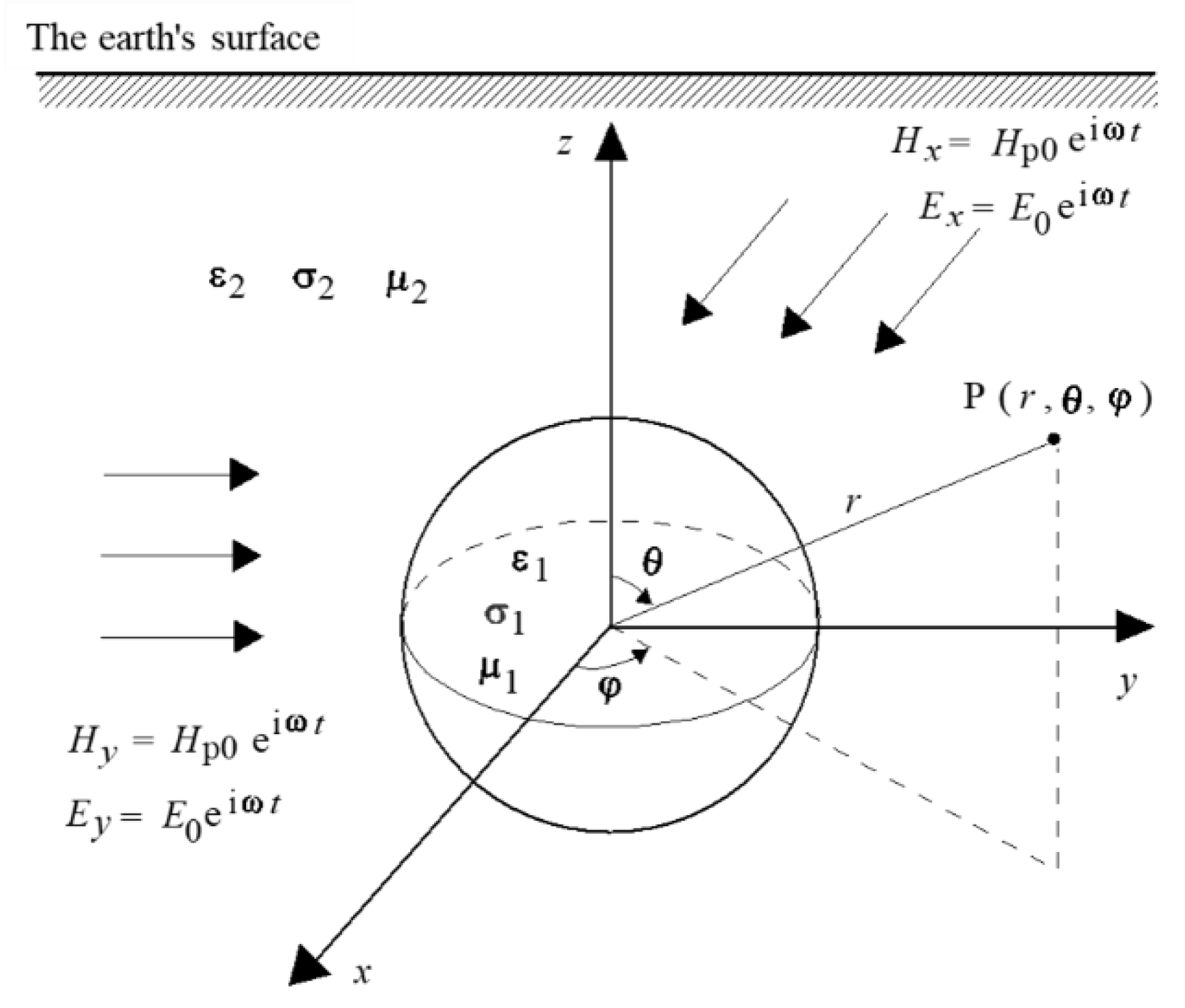
The author has made forward analysis on the causes of profile anomalies of FSM in recent years [27,28,29]. In this paper, the cause of anomaly in FSM sounding is also discussed with a simple sphere in homogeneous half space. For a conductive and magnetic spheres in the uniform half space medium as shown in Figure 5, the sphere is a, and its dielectric constant, electrical conductivity, and permeability are ε₁, σ₁, and μ₁, respectively. The corresponding parameters of surrounding rocks are ε₂, σ₂, and μ₂. According to the past research results, when FSM is used for exploration, only the natural primary electromagnetic field components, namely the horizontal alternating electric field E_x, E_y and the horizontal alternating magnetic field H_x, H_y act on the sphere, which come from the far field. To simplify the problem, it is assumed that E_x = E_y = E₀ × e^iωt, H_x = H_y = H_p0 × e^iωt. Here ω is a circular frequency and ω = 2πf, and f is the frequency. The coordinates of the observation points are P(r, θ, φ) in the spherical coordinate system, as shown in Figure 5.

In the medium with electrical conductivity σ ≠ 0, the free charge cannot be stacked in a certain place, so that the propagation of the magnetotelluric fields obeys the Maxwell’s equations. Four-vector fields: the electric field E, the magnetic field H, the electric introduction D, and the magnetic introduction B satisfy following equations:

$$\nabla \times \mathit{E}=-\mu \cdot \frac{\partial \mathit{H}}{\partial t}$$

(1)

$$\nabla \times \mathit{H}=\sigma \cdot \mathit{E}+\epsilon \cdot \frac{\partial \mathit{E}}{\partial t}$$

(2)

$$\nabla \cdot \mathit{D}=0$$

(3)

$$\nabla \cdot \mathit{B}=0$$

(4)

By using the separation variable method [27,28,29], the components of secondary electric field outside the sphere which produced by the primary magnetic field component Hx are given in Equations (5) and (6).

$$E_{2y}=-\left[C_1{J}_{3/2}\left(k_{2}r\right)+D_1{J}_{-3/2}\left(k_{2}r\right)\right]\frac{1}{\sqrt{k_{2}r}}\frac{z}{\sqrt{x^2+y^2+z^2}}$$

(5)

$$E_{2z}=\left[C_1{J}_{3/2}\left(k_{2}r\right)+D_1{J}_{-3/2}\left(k_{2}r\right)\right]\frac{1}{\sqrt{k_{2}r}}\frac{y}{\sqrt{x^2+y^2+z^2}}$$

(6)

Similarly, the components of secondary electric field outside the sphere generated by the primary magnetic field component H_y are given in Equations (7) and (8).

$$E_{2z}=-\left[C_1{J}_{3/2}\left(k_{2}r\right)+D_1{J}_{-3/2}\left(k_{2}r\right)\right]\frac{1}{\sqrt{k_{2}r}}\frac{x}{\sqrt{x^2+y^2+z^2}}$$

(7)

$$E_{2x}=\left[C_1{J}_{3/2}\left(k_{2}r\right)+D_1{J}_{-3/2}\left(k_{2}r\right)\right]\frac{1}{\sqrt{k_{2}r}}\frac{z}{\sqrt{x^2+y^2+z^2}}$$

(8)

where J_3/2(kr) and J_−3/2(kr) are the complex argument Bessel function, and k₂ is the wave number of surrounding rock, k₂² = ω²ε₂μ₂ − iωμ₂σ₂, i is imaginary unit, and i² = −1. The coefficients C₁, D₁ are written as:

$$C_1=-\frac{i\omega 3\sqrt{\pi }{\mu }_1{\mu }_2{H}_P{k}_1^2{a}^3}{2\sqrt{2}\left\{\left({\mu }_2{-\mu }_1\right)p_1{\cos p}_1-\left[{\mu }_2\left({1-p}_1^2\right){-\mu }_1\right]{\sin p}_1\right\}}$$

$$D_1=-\frac{a^3}{2\sqrt{2}}\frac{\left(2{\mu }_1+{\mu }_2\right)p_1\cos p_1-\left[{\mu }_2\left(1-p_1^2\right)+2{\mu }_1\right]\sin p_1}{\left({\mu }_2-{\mu }_1\right)p_1\cos p_1-\left[{\mu }_2\left(1-p_1^2\right)-{\mu }_1\right]\sin p_1}i\omega \sqrt{\pi }{\mu }_2{k}_2^2{H}_P$$

In the above two equations, p₁ = k₁a, k₁ is the wave number of spherical media. If the displacement current is ignored, k₁² = −iωμ₁σ₁.

For the effect of two horizontal alternating electric field E₀ × e^iω⋅t in the horizontal direction in Figure 5, the solution can be approximately obtained by referring a conducting sphere in the uniform electrostatic field. If only the anomaly field is considered, the potential distribution of the anomalous field outside the sphere is written as:

$$U_p=2\frac{{\sigma }_1-{\sigma }_2}{{\sigma }_1+2{\sigma }_2}{\left(\frac{a}{r}\right)}^3\frac{j_0}{{\sigma }_2}r\sin \theta {\mathsf{e}}^{i\omega \cdot t}$$

(9)

According to Equation (9), the components of induced secondary electric field E_2y, E_2x on the main surface profile along the y axis (x = 0) in the rectangular coordinate system are calculated by Equations (10) and (11).

$$E_{2y}=2\frac{{\sigma }_1-{\sigma }_2}{{\sigma }_1+2{\sigma }_2}{a}^3\frac{j_0}{{\sigma }_2}\frac{2y^2-h_0^2}{{\left(y^2+h_0^2\right)}^{5/2}}{\mathsf{e}}^{i\omega \cdot t}$$

(10)

$$E_{2x}=2\frac{{\sigma }_1-{\sigma }_2}{{\sigma }_1+2{\sigma }_2}{a}^3\frac{j_0}{{\sigma }_2}\frac{-1}{{\left(y^2+h_0^2\right)}^{3/2}}{\mathsf{e}}^{i\omega \cdot t}$$

(11)

where h₀ is the center point depth of the sphere, j₀ = E₀/ρ₂.

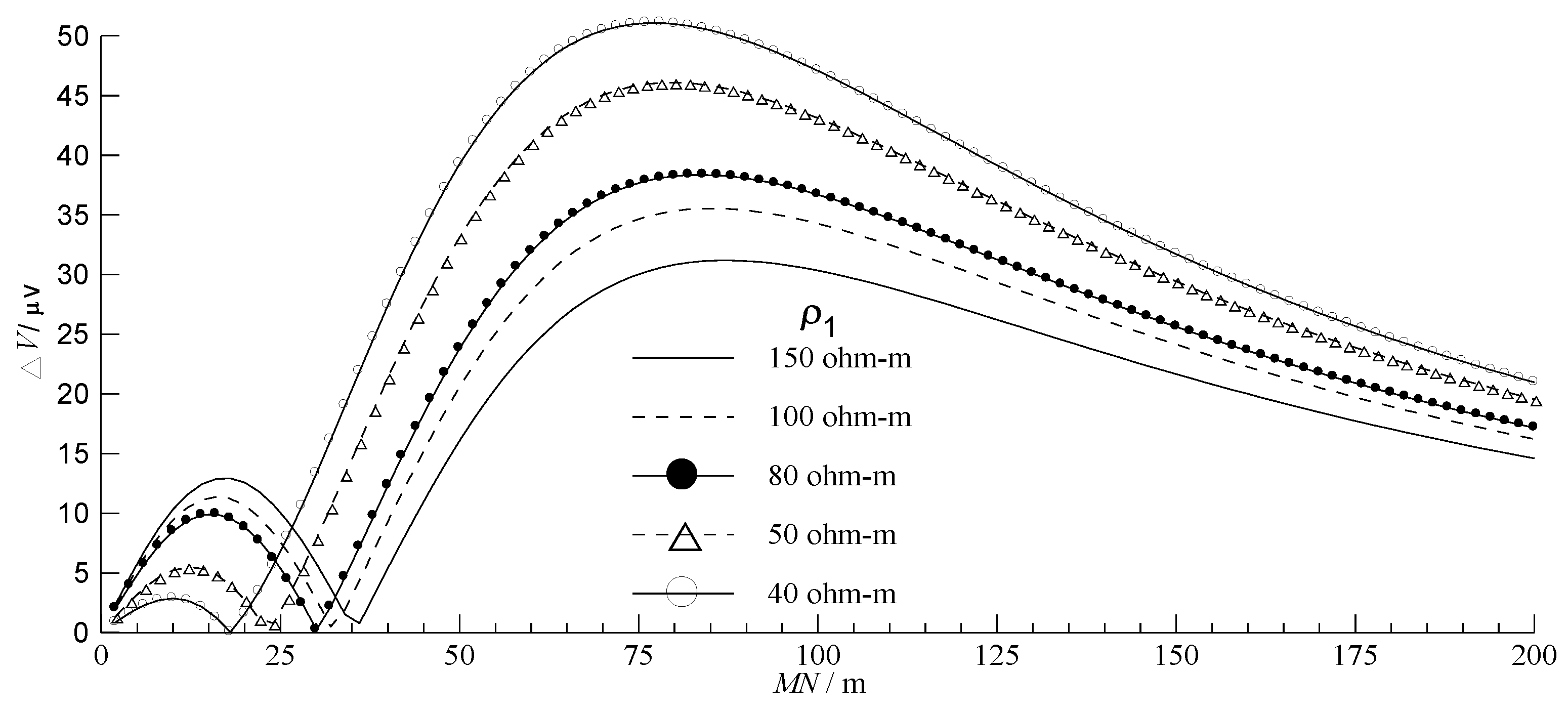
Assume that f = 170 Hz, h₀ = 30 m, a = 1 m, ρ₁ = 150 ohm-m, ρ₂ = 2500 ohm-m, B₀ = 1 × e^iω⋅t T, and E₀ = 25 × 10⁻³ × e^iω⋅t V/m in the model shown in Figure 5. Here, ρ₁ and ρ₂ are resistivity of the sphere and the surrounding rock, respectively. It is assumed that the surrounding rock and the sphere are both nonmagnetic. Therefore, the secondary abnormal electric field potential difference ΔV of FSM sounding on the surface main profile along the y direction can be calculated by using Equations (5) and (10). Figure 6 reflects the variation of potential difference ΔV of FSM sounding with the magnitude of the electrode spacing MN and resistivity ρ₁ of the sphere, and the step length of MN in calculation process is 2 m. Because we are mainly interested in abnormal fields in electrical exploration, only the abnormal secondary electric field potential difference is plotted in Figure 6, and the primary electric field is not included. However, the measured results in Figure 4b contain the primary field. Since the primary field is considered to be a uniform field, its potential difference increases with the electrode spacing MN, and its curve is a slanted straight line.

It can be seen that the anomalous electric field potential difference appears obvious relative low potential anomaly at MN = 36 m in Figure 6 when ρ₁ = 150 ohm-m, and the ratio of the anomalous polar distance (MN = 36 m) to the center point depth of the sphere (h₀ = 30 m) is 1.2. Assuming that only the resistivity ρ₁ of sphere is changed in the above model, as shown in

Table 2. Ratios of MN/h₀ at abnormal points of FSM sounding curve with different resistivity ρ₁ of sphere.

ρ1 (Ω·m)	150	100	80	50	40
MN of abnormal point position (m)	36	32	30	24	18
MN/h0	1.20	1.07	1.00	0.80	0.60

, the shape of sounding curve of anomalous electric field remains unchanged (Figure 6), but the position of relative low potential anomaly will change (Figure 6, Table 2). The ratio MN/h₀ at abnormal points of sounding curve decreases with the decrease of resistivity ρ₁.

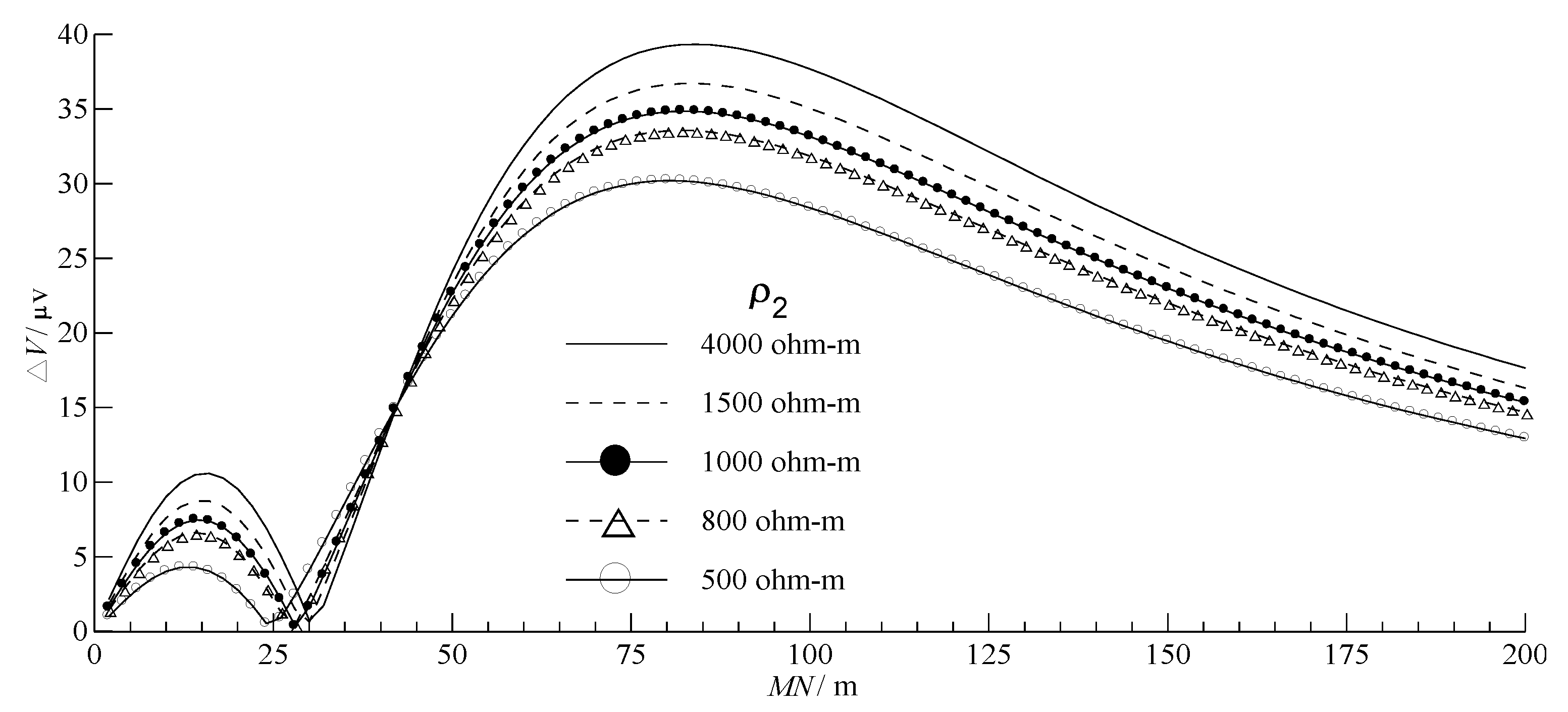
Similarly, assuming that parameters of the model are f = 170 Hz, h₀ = 30 m, a = 1, ρ₁ = 80 ohm-m, B₀ = 1 × e ^iω⋅t T and E₀ = 25 × 10⁻³ × e^iω⋅t V/m, and only the resistivity ρ₂ of the surrounding rock is changed, as shown in

Table 3. Ratios of MN/h₀ at abnormal points of FSM sounding curve with different resistivity ρ₂ of surrounding rock.

ρ2 (Ω·m)	4000	1500	1000	800	500
MN of abnormal point position (m)	30	30	28	28	24
MN/h0	1.00	1.00	0.933	0.933	0.80

(forward calculating curves of FSM are shown in Figure 7), when ρ₂ is 4000 ohm-m or 1500 ohm-m, the relative low potential anomaly appears at MN = 30 m, and the ratio MN/h₀ at abnormal point of sounding curve is 1.0. In general, the ratio MN/h₀ decreases with the decrease of resistivity ρ_2, as shown in Table 3.

According to the calculating results in Table 2 and Table 3, the ratio MN/h₀ at relative low potential abnormal point varies approximately around 1.0. This is in agreement with the practical application results in Table 1.

5. Conclusions

Statistical analysis of drilling results in 98 typical borehole wells shows that there is an approximate 1:1 relationship between the potential electrode spacing MN and the depth of aquifer at the relative low potential abnormal point of FSM sounding curves. This empirical relationship has a certain guiding role for future practice. Finally, the author carried out forward research on the FSM sounding method. A simplified geophysical model of a low resistance conductive sphere in a homogeneous half space was used in the study, and the secondary anomalous electric field on the surface main profile was calculated when the sphere was under the combined action of the horizontal alternating electromagnetic fields. Forward calculation results show that there will be a relatively low potential anomaly point in FSM sounding curve when the resistivity of the sphere is approximately equal to that of groundwater, and the ratio of electrode spacing (MN) to the center point depth (h₀) of the sphere at the relatively low potential anomaly point of sounding curves varies approximately around 1.0. The theoretical calculation results are in good agreement with the statistical results of practical application, which also explains the cause of anomaly of FSM sounding method.

The theoretical research indicates that the cause of FSM anomaly is the comprehensive effect of the natural 3D alternating electromagnetic signal underground. According to the application of FSM in the 12th Five-Year Plan of rural drinking water safety project in Guangxi Province, there are 114 boreholes with water yield more than 1 m³/h, and the success rate is about 87.0%. This shows that FSM has obvious effectiveness in shallow (depth < 150 m) groundwater exploration, and it is an effective method to identify suitable borehole sites of groundwater in the future.

FSM belongs to the natural passive source method, and its field source is very complex. In this paper, the author used only a very simple geophysical model to discuss the anomaly of the FSM sounding curve, which is just a function of throwing out a brick to attract a jade. There are many related problems of FSM to be further studied in the future.

References

- Yang, T.C.; Xia, D.L.; Wang, Q.R.; Fu, G.H. Theoretical Research and Application of Natural Electric Field Frequency Selection Method; Central South University Press: Changsha, China, 2017. [Google Scholar]
- Bao, G.S.; Li, D.Q.; Zhang, Y.S.; Wang, S.W. Research on the interfering electric field instrument. Chin. J. Nonferrous Met. 1994, 4, 9–13. [Google Scholar]
- Zhang, J.; Li, K.; Huang, C.L.; Li, Z.Y. Detecting system of underground magneto fluid & application. Comput. Technol. Autom. 2010, 29, 119–122, 136. [Google Scholar]
- Wang, R.G.; Liu, S.Y.; Shangguan, D.H.; Radic, V.; Zhang, Y. Spatial Heterogeneity in Glacier Mass-Balance Sensitivity across High Mounta in Asia. Water 2019, 11, 776. [Google Scholar] [CrossRef] [Green Version]
- Deng, R.J.; Shao, R.; Ren, B.Z.; Hou, B.L.; Tang, Z.E.; Hursthouse, A. Adsorption of Antimony(III) onto Fe(III)-Treated Humus Sludge Adsorbent: Behavior and Mechanism Insights. Pol. J. Environ. Stud. 2019, 28, 577–586. [Google Scholar] [CrossRef] [PubMed]
- Zhang, Y.; Ren, B.Z.; Hursthouse, A.; Deng, R.J.; Hou, B.L. Leaching and Releasing Characteristics and Regularities of Sb and As from Antimony Mining Waste Rocks. Pol. J. Environ. Stud. 2019, 28, 4017–4025. [Google Scholar] [CrossRef] [PubMed]
- You, B.; Xu, J.X.; Shi, S.L.; Liu, H.Q.; Lu, Y.; Liang, X.Y. Treatment of coal mine sewage by catalytic supercritical water oxidation. Fresenius Environ. Bull. 2020, 29, 497–502. [Google Scholar]
- Yu, S.Q.; Mo, Q.F.; Chen, Y.Q.; Li, Y.W.; Li, Y.X.; Zou, B.; Xia, H.P.; Jun, W.; Li, Z.A.; Wang, F.M. Effects of seasonal precipitation change on soil respiration processes in a seasonally dry tropical forest. Ecol. Evol. 2020, 10, 467–479. [Google Scholar] [CrossRef] [Green Version]
- Wang, Z.H.; Huang, W.; Wang, C.; Li, X.S.; He, Z.H.; Hursthouse, A.; Zhu, G.C. Variation of Al species during water treatment: Correlation with treatment efficiency under varied hydraulic conditions. AQUA Water Infrastruct. Ecosyst. Soc. 2021, 70, 891–900. [Google Scholar] [CrossRef]
- Zhang, J.; Huang, C.L.; Wang, J.; Zhou, H. Detecting system of underground magneto fluid and its application on mine area flood prevention. Chin. J. Sci. Instrum. 2009, 30 (Suppl. S6), 807–810. [Google Scholar]
- Cheng, H.; Bai, Y.C. Design and application of audio frequency natural electric field instrument. Prog. Geophys. 2014, 29, 2874–2879. [Google Scholar]
- Zhang, K.Y.; Zhou, M.R.; Yan, P.C.; Wang, R. Research of electrical conductivity measurement system based on frequency selection method. Instrum. Tech. Sens. 2015, 42, 65–67. [Google Scholar]
- Zhao, Y.L.; Luo, S.L.; Wang, Y.X.; Wang, W.J.; Zhang, L.Y.; Wan, W. Numerical analysis of karst water inrush and a criterion for establishing the width of water-resistant rock pillars. Mine Water Environ. 2017, 36, 508–519. [Google Scholar] [CrossRef]
- Yang, T.C.; Zhang, Y.P.; Fu, G.H. Application research of comprehensive geophysical method to karst investigaion in a productive mine. Prog. Geophys. 2021, 36, 1145–1153. [Google Scholar]
- Yang, Z.C. The least-square Fourier-series model-based evaluation and forecasting of monthly average water-levels. Environ. Earth Sci. 2018, 77, 328. [Google Scholar] [CrossRef]
- Jin, C.S.; Liu, Y.X.; Li, Z.W.; Gong, R.Z.; Huang, M.; Wen, J.J. Ecological consequences of China’s regional development strategy: Evidence from water ecological footprint in Yangtze River Economic Belt. Environ. Earth Sci. 2018, 77, 328. [Google Scholar] [CrossRef]
- Zhou, J.Z.; Zhang, M.Q.; Ji, M.T.; Wang, Z.H.; Hou, H.; Zhang, J.; Huang, X.; Hursthouse, A.; Qian, G.R. Evaluation of heavy metals stability and phosphate mobility in the remediation of sediment by calcium nitrate. Water Environ. Res. 2020, 92, 1017–1026. [Google Scholar] [CrossRef] [PubMed]
- Berdychevsky, M.H. Telluric Current Prospecting; China Industrial Press: Beijing, China, 1962. [Google Scholar]
- Pham, V.N.; Boyer, D.; Xue, C.Y.; Liu, S.C. Application of telluric-telluric profiling combined with magnetotelluric and self-potential methods to geothermal exploration in the Fujian Province, China. J. Volcanol. Geotherm. Res. 1995, 65, 227–236. [Google Scholar] [CrossRef]
- Mlynarski, M.; Zlotnicki, J. Fluid circulation in the active emerged Asal rift (east Africa, Djibouti) inferred from self-potential and Telluric-Telluric Prospecting. Tectonophysics 2001, 339, 455–472. [Google Scholar] [CrossRef]
- Deng, R.J.; Jin, C.S.; Ren, B.Z.; Hou, B.L.; Hursthouse, A.S. The Potential for the Treatment of Antimony-Containing Wastewater by Iron-Based Adsorbents. Wate 2017, 9, 794. [Google Scholar] [CrossRef] [Green Version]
- Wang, P.F.; Tan, X.H.; Zhang, L.Y.; Li, Y.J.; Liu, R.H. Influence of particle diameter on the wettability of coal dust and the dust suppression efficiency via spraying. Process Saf. Environ. Prot. 2019, 132, 189–199. [Google Scholar] [CrossRef]
- Liu, T.; Chen, Z.S.; Li, Z.X.; Fu, H.; Chen, G.L.; Feng, T.; Chen, Z. Preparation of magnetic hydrochar derived from iron-rich Phytolacca acinosa Roxb. for Cd removal. Sci. Total Environ. 2021, 769, 145–159. [Google Scholar] [CrossRef] [PubMed]
- Yang, T.C.; Zhang, H. Study faults by natural electric field frequency selection method. J. Hunan Univ. Sci. Technol. (Nat. Sci. Ed.) 2013, 28, 32–37. [Google Scholar]
- Yang, T.C.; Zhang, H. A study of the anomaly genesis for the frequency selection method in a natural electric field of a karst body. Hydrogeol. Eng. Geol. 2013, 40, 22–28. [Google Scholar]
- Yang, T.C.; Shen, J.P.; Li, G.M.; Cao, Y.J.; Zhang, H. Application and analysis of natural electric field frequency selection method for water-filled karst investigation. Coal Geol. Explor. 2014, 42, 71–75. [Google Scholar]
- Yang, T.C.; Zhang, Q.; Wang, Q.R.; Fu, G.H.; Liao, J.P. Study on the anomaly genesis of the frequency selection method for a sphere under natural electromagnetic field. J. Hunan Univ. Sci. Technol. (Nat. Sci. Ed.) 2016, 31, 58–65. [Google Scholar]
- Chen, Z.C.; Deng, H.Y.; Yang, T.C. The observation and test of the daily variation based on the frequency selection method of natural electtric field. Miner. Eng. Res. 2020, 35, 61–66. [Google Scholar]
- Yang, T.C.; Liang, J.; Cheng, H.; Cao, S.J.; Dong, S.Y.; Gong, Y.F. The effect and the anomaly analysis of shallow groundwater exploration based on the frequency selection method of natural electric field. Geophys. Geochem. Explor. 2018, 42, 1194–1200. [Google Scholar]
- Zhou, Y.Y.; Ren, B.Z.; Hursthouse, A.S.; Zhou, S.J. Antimony Ore Tailings: Heavy Metals, Chemical Speciation, and Leaching Characteristics. Pol. J. Environ. Stud. 2019, 28, 485–495. [Google Scholar] [CrossRef]
- Hou, B.L.; Liu, X.; Li, Z.; Ren, B.Z.; Kuang, Y. Heterogeneous fenton oxidation of butyl xanthate catalyzed by iron-loaded sewage sludge. Fresenius Environ. Bull. 2022, 31, 4125–4131. [Google Scholar]
- Tang, J.T.; Zhou, C.; Xiao, X. Selection of minimum transmit-receive distance of CSAMT on complicated media. Chin. J. Nonferrous Met. 2013, 23, 1681–1693. [Google Scholar]
- Shi, X.Y.; Ren, B.Z.; Hursthouse, A. Source identification and groundwater health risk assessment of PTEs in the stormwater runoff in an abandoned mining area. Environ. Geochem. Health 2022, 44, 3555–3570. [Google Scholar] [CrossRef] [PubMed]
- Yuan, Q.; Zhu, G.C. A review on metal organic frameworks (MOFs) modified membrane for remediation of water pollution. Environ. Eng. Res. 2021, 26, 190435. [Google Scholar] [CrossRef]
- Zhao, Y.L.; Zhang, C.S.; Wang, Y.X.; Lin, H. Shear-related roughness classification and strength model of natural rock joint based on fuzzy comprehensive evaluation. Int. J. Rock Mech. Min. Sci. 2021, 137, 104550. [Google Scholar] [CrossRef]
- Liu, J.H.; Zhao, Y.L.; Tan, T.; Zhang, L.Y.; Zhu, S.T.; Xu, F.Y. Evolution and modeling of mine water inflow and hazard characteristics in southern coalfields of China: A case of Meitanba mine. Int. J. Min. Sci. Technol. 2022. [CrossRef]
- Chongo, M.; Christiansen, A.V.; Tembo, A.; Banda, K.E.; Imasiku, A.N.; Larsen, F.; Peter, B.G. Airborne and ground-based transient electromagnetic mapping of groundwater salinity in the Machile-Zambezi Basin, southwestern Zambia. Near Surf. Geophys. 2015, 13, 383–395. [Google Scholar] [CrossRef]
- Ikard, S.; Pease, E. Preferential groundwater seepage in karst terrane inferred from geoelectric measurements. Near Surf. Geophys. 2019, 17, 43–53. [Google Scholar] [CrossRef] [Green Version]
- Tian, Z.J.; Zhang, Z.Z.; Deng, M.; Yan, S.; Bai, J.J. Gob-Side Entry Retained with Soft Roof, Floor, and Seam in Thin Coal Seams: A Case Study. Sustainability 2020, 12, 1197. [Google Scholar] [CrossRef] [Green Version]
- Zhang, Y.; Huang, F.Y. Indicative significance of the magnetic susceptibility of substrate sludge to heavy metal pollution of urban lakes. ScienceAsia 2021, 47, 374. [Google Scholar] [CrossRef]
- Yang, J. Experimental results and theoretical study of the stray current method in karst area. Geophys. Geochem. Explor. 1982, 6, 41–54. [Google Scholar]
- Li, Y.C.; Hu, X.X.; Ren, B.Z. Treatment of antimony mine drainage: Challenges and opportunities with special emphasis on mineral adsorption and sulfate reducing bacteria. Water Sci. Technol. 2016, 73, 2039–2051. [Google Scholar] [CrossRef]
- Li, Y.C.; Xu, Z.; Ma, H.Q.; Hursthouse, A. Removal of Manganese(II) from Acid Mine Wastewater: A Review of the Challenges and Opportunities with Special Emphasis on Mn-Oxidizing Bacteria and Microalgae. Wate 2019, 11, 2493. [Google Scholar] [CrossRef] [Green Version]
- Zheng, C.S.; Jiang, B.Y.; Xue, S.; Chen, Z.W.; Li, H. Coalbed methane emissions and drainage methods in underground mining for mining safety and environmental benefits: A review. Process Saf. Environ. Prot. 2019, 127, 103–124. [Google Scholar] [CrossRef]
- Qin, B.T.; Li, L.; Ma, D.; Lu, Y.; Zhong, X.X.; Jia, Y.W. Control technology for the avoidance of the simultaneous occurrence of a methane explosion and spontaneous coal combustion in a coal mine: A case study. Process Saf. Environ. Prot. 2016, 103, 203–211. [Google Scholar] [CrossRef]
- Liang, J.; Wei, Q.F.; Hong, J.; Zheng, S.Y.; Qin, Y.C.; Yan, F.S.; Feng, Y.X. Application of self-potential method to explore water in karst area. Geotech. Investig. Surv. 2016, 44, 68–78. [Google Scholar]
- Zhao, Y.L.; Liu, Q.; Zhang, C.S.; Liao, J.; Lin, H.; Wang, Y.X. Coupled seepage-damage effect in fractured rock masses: Model development and a case study. Int. J. Rock Mech. Min. Sci. 2021, 144, 104822. [Google Scholar] [CrossRef]
- Zhao, Y.L.; Zhang, L.Y.; Wang, W.J.; Tang, J.Z.; Lin, H.; Wan, W. Transient pulse test and morphological analysis of single rock fractures. Int. J. Rock Mech. Min. Sci. 2017, 91, 139–154. [Google Scholar] [CrossRef]
Figure 1.
Map showing the location of FSM application in Guangxi study area. (a) The location of the study province in China. (b) The enlarged map of the study province.
Figure 2.
Regional geological map showing the location of FSM in Guangxi study area.
Figure 3.
(a) A schematic diagram of a profile detection device and (b) a sounding device of FSM.
Figure 4.
(a) Profile survey results and (b) sounding results of FSM in Chetian village.
Figure 5.
A sphere in natural alternating electromagnetic field in half space.
Figure 6.
Forward calculating curves of FSM sounding for different resistivity ρ1.
Figure 7.
Forward calculating curves of FSM sounding for different resistivity ρ2.