An Integrated Approach to Evaluating Crop Water Requirements and Irrigation Schedule for Optimizing Furrow Irrigation Design Parameters in Kurnool District, India

Abstract

In Kurnool district, due to the hot, arid climatic conditions, proper study of crop evapotranspiration and its effect on crop water demand for various crops is an extremely important issue. More focus will be given to the design and development of surface irrigation systems based mostly on furrow irrigation, as the rainfall pattern for this district was irregular in 2005. The crop water requirement and furrow irrigation design parameters for optimising the beneficial utilisation of available water resources and field performances are studied in this research. Some major crops, such as cotton, sugarcane, sorghum, maize, and sunflower, are considered when adopting a suitable furrow irrigation system for soil conditions of the types black clay, red loamy, and medium loam. The reference crop evapotranspiration was estimated for 2005 based on the Penman–Monteith equation as per FAO guidelines by the CROPWAT 8.0 model. Crop Water Requirement (CWR), Net Irrigation Requirement (NIR), and Gross Irrigation Requirement (GIR) were determined for available climatic and soil conditions. Soil surface characteristics were studied using AQUACROP 6.1 and compared with CROPWAT 8.0 for model accuracy. Various conservative and non-conservative crop characteristics were studied under limited set conditions, and correlation equations were developed between different parameters. Moreover, different furrow irrigation design parameters were considered by FURDEV (a module of the SURDEV model) for three modes of operation (i.e., fixed flow, cutback flow, and tailwater reuse method) under modified SCS (Soil Conservation Service) families of soil infiltration characteristics. NIR values were 200 mm, 1423.2 mm, 220 mm, 150 mm, and 150 mm for cotton, sugarcane, maize, sorghum, and sunflower, respectively. A maximum significant dry yield was observed for maize (13.586 tonnes/ha). Additionally, the maximum application efficiency and storage efficiency were obtained at 95.5% for sorghum and 99.3% for sunflower, which would be a beneficial outcome of this research. In general, the results of this research might be very effective for the irrigation authority of Kurnool District to plan suitable approaches for designing and developing proper water management systems.

1. Introduction

Due to the current population increase, a shortage of food might be observed in the future. Therefore, it is a very important issue to ensure food security by increasing crop productivity in a more advanced technical manner and to design and develop suitable arrangements to allow the growth of crops in a well-managed way under the existing climatic and environmental conditions. The rainfall pattern for Kurnool district, in India, was insufficient and irregular in 2005. A very small amount of rainfall (only 11 mm) occurred during the winter season (i.e., from January to March). Most of the crops were rabi crops, which faced significant soil moisture stress at the root zone. Then, a considerable quantity of water from irrigation was distributed to meet the low crop productivity.

It is important that the water demands of various crops are studied at different management levels to achieve effective irrigation management [1]. Therefore, evaluation of crop evapotranspiration and crop water requirement (CWR) with high accuracy and precision is a challenging issue, mainly in some arid and semi-arid regions. Irrigation is an important and costly input in agriculture consisting of high management and field accuracy for increasing food production. Several computer models are now available, such as CROPWAT 8.0, for proper assessment of CWR and irrigation schedules [2]. It is calculated from effective rainfall, available climatic and meteorological parameters, and soil moisture conditions [3]. CROPWAT 8.0 also simulates reference crop evapotranspiration soil characteristics and is responsible for showing cropping patterns under different rainfed and non-rainfed conditions over the available irrigated area [4,5]. Crop water demand is obtained by the product of estimated reference crop evapotranspiration and crop coefficient (K_c) based on different crop growth stages [6]. K_c mainly depends on crop type and its growth period, soil water condition, frequency of irrigation, canopy development, leaf area index (LAI), etc. [7,8]. Crop evapotranspiration can be determined from the climatic data by directly integrating the crop resistance, albedo, and air resistance factors in the Penman–Monteith approach [9]. Actual evapotranspiration (ET_a) is determined by taking into account the stress function (i.e., water stress coefficient K_s, so that ET_a = K_s·ET_o) depending on the actual moisture content at the root zone [10]. Therefore, planning and management of irrigation water from different sources are most important in the arid and semi-arid regions. For that, proper evaluation of CWR can be effectively understood for better and more efficient utilisation and conservation of irrigation water [11]. The Indian economy is highly dependent on agriculture, and water is a key element in agriculture [12]. So, the productivity of crops should be enhanced with the minimum utilisation of available surface water and groundwater resources. Improper irrigation management and water estimation are two of the main reasons for increasing irrigated area, as well as poor growth and development of crops, and are responsible for reductions in crop yield [13]. Factors like poor soil fertility, increased soil salinity, overapplication of fertilisers, and poor field management may limit crop production and crop evapotranspiration [14].

In Kurnool district, irrigation is mainly carried out from canals, tanks, tube wells, and some other sources. The crops studied in the present research are generally cultivated by furrow irrigation. Improvement of water productivity in furrow irrigation can be achieved by proper application of this water at the right time with an accurate flow rate [15]. This basically consists of proper design of furrow length, irrigation timings, and furrow cross-sections [16]. Discharge and furrow length are two major elements that increase irrigation efficiency, and furrow irrigation is widely adopted as a form of surface irrigation [17]. There are so many methods for designing and developing surface irrigation systems [18]. SURDEV is one of the most effective platforms for planning and designing border, basin, and furrow irrigation. FURDEV is used for furrow irrigation [18,19].

To determine the furrow irrigation design parameters accurately and to obtain an attainable yield for the crops, FAO has developed a yield response to a water model called AQUACROP. Different conservative and non-conservative crop parameters such as canopy development, canopy senescence, root zone expansion, biomass, harvestable yield, flowering, and potential vegetative growth stage are important physiological crop responses to water stress [8,20]. It also provides information on different soil characteristics along different soil horizons.

From the above literature, it is concluded that most of the researchers have focused on the determination of the crop water requirement, gross and net irrigation requirement, and irrigation scheduling for different types of crops under different soil and climatic conditions. Moreover, in some studies, furrow irrigation design parameters were being discussed from different perspectives. The use of various programmes and software such as SAS 9.2 [21], CROPWAT 8.0, and CLIMWAT 2.0 had been studied, which would provide a lot of knowledge and ideas. However, the crop characteristics, conservative and non-conservative crop parameters, crop phenology, biomass production, and crop yield, along with the proper irrigation method to develop a well-designed irrigation system and control the use of water, were not evaluated in the past studies.

Therefore, the objectives of this study are: (i) to estimate the reference crop evapotranspiration and the crop evapotranspiration under standard conditions for the studied crops under a single crop coefficient approach; (ii) to determine the crop water requirement and the net and gross irrigation requirements under various field conditions and to show the contribution of effective rainfall; (iii) to obtain the soil surface characteristics and to develop an inter-relation between them and the crop characteristics; and (iv) to obtain suitable furrow irrigation design parameters under existing field management and climatic conditions.

2. Materials and Methods

2.1. Study Area

The study area is the Kurnool District in India. Its location map is shown in Figure 1. The district has an altitude of 95 m above sea level (a.s.l.), Latitude 14°54′ and 16°18′ N and Longitude 76°58′ and 79°34′ E. The mean monthly temperature ranges from 36 °C in the summer to 21.5 °C in the winter season. The climate in this area is tropical. The major soil types are basically black clay soil, red loamy soil, and medium soil (loam soil). The major sources of irrigation water are usually canals and tube wells. The planting date, harvesting date, and type of soil for the studied crops are tabulated below (

Table 1. Planting date, harvesting date, and type of soil for the crops under study.

Crops	Planting Date	Harvesting Date	Type of Soil
Cotton	03/08/2005	29/01/2006	Black Clay Soil
Sugarcane	15/09/2005	14/09/2006	Medium (Loam) Soil
Maize	07/05/2005	08/09/2005	Red Loamy Soil
Sorghum	06/11/2005	05/03/2006	Red Loamy Soil
Sunflower	28/01/2005	06/06/2005	Red Loamy Soil

).

2.2. Meteorological Data

Meteorological and climatic data for the Kurnool district from 1 January to 31 December 2005 were taken from CLIMWAT 2.0. The data was available only for this year. However, the present work—albeit with some limitations—tries to perform long-term variations of the meteorological and climatic parameters with their effects on reference crop evapotranspiration and crop production as well. The monthly maximum and minimum temperature (°C), relative humidity (%), sunshine radiation (MJ/m²/day), wind speed (km/day), and rainfall value (mm) were used as input to estimate the reference crop evapotranspiration (ET_o) in mm/day from the Penman–Monteith equation (Equation (1)) as per FAO guidelines by CROPWAT 8.0 [14]:

ET_o = [0.408∆(Rn − G) + γ900/(T + 273) (e_s − e_a)u₂]/[∆ + γ(1 + 0.34u₂)]

(1)

where ∆ = slope of the saturation vapour pressure versus temperature curve (KPa/°C), Rn = net heat radiation (MJ/m²/day), G = soil heat flux (MJ/m²/day), γ = pschycometric constant (KPa/°C), (e_s − e_a) = saturation vapour pressure deficit (KPa), T = mean air temperature in (°C), and u₂ = wind speed at a height of 2 m from the ground surface (m/s).

The Leaf Area Index (LAI) is an important parameter used to calculate the surface resistance (r_s), which is a key factor in the Penman–Monteith equation. It is basically calculated by Equation (2) based on FAO Irrigation and Drainage Paper 56, as given below [14]:

LAI = 24·h

(2)

where LAI is the leaf area index (m²/m²) and h is the crop height (m) and can be estimated through the FAO Irrigation and Drainage Paper 56 [14]. CROPWAT 8.0 performs the determination of LAI according to the FAO guidelines. However, for obtaining seasonal variation in canopy cover and plant growth, LAI plays a key role, and its determination may include some direct and indirect measurements.

CROPWAT 8.0 also simulates crop water requirements, cropping patterns, and irrigation scheduling for daily moisture balance and crop evapotranspiration under both standard and non-standard situations for different soil, climatic, and crop conditions. The irrigation scheduling for the crops under study was performed by CROPWAT 8.0 using the irrigation timings and irrigation application as follows: (a) irrigation at a fixed interval per crop growing stage; (b) fixed application depth; (c) refill soil at field capacity; and (d) irrigation at critical depletion. In the present study, the fixed percentage method to calculate the effective rainfall as described in Equation (3) was used [22]:

P_eff = a·P_total

(3)

where P_eff is the effective rainfall (mm), a (which is a user-defined parameter) is the fraction of total rainfall getting converted into P_eff, and P_total is the total rainfall (mm).

2.3. Crop Data

The crop data consisting of crop growing period (planting and harvesting time), crop height, and suitable soil were taken from the irrigation profile of the Kurnool District (Agriculture Contingency Plan of Kurnool District). The crop coefficients (K_c) at different growth stages (i.e., initial stage, crop development, mid-season stage, and late season stage) were taken from FAO Irrigation and Drainage Paper 56 [14].

The simulation of crop evapotranspiration, ET_c, was performed under non-water stress conditions, without the application of fertilisers, growth of weeds, or adverse field management conditions. ET_c was calculated by associating the crop coefficient (K_c) to ET_o. During the initial period of the crop growth stage, only a very small canopy covers the ground surface. So, a lower value of K_c was found at this growing period with a shorter growing length. At the crop development stage, almost the maximum canopy covers the ground (i.e., 70–80% of the ground). The mid-season stage lasted after crop development until the crop attained full maturity. The maximum height, the building of the Harvest Index (HI), and flowering started at this phase. The K_c value will also increase, and it is affected by wind speed and relative humidity. K_c,mid (i.e., K_c at the mid-season stage) and K_c,end (i.e., K_c at the end stage) values can be adjusted according to the climatic parameters when the minimum relative humidity is more than 45% and the wind speed is more than 2 m/s [14] as follows:

K_c,mid,adj = K_c,mid,table + [0.04(u₂ − 2) − 0.004(RH_min − 45)](h/3)^0.3

(4)

K_c,end,adj= K_c,end,table + [0.04(u₂ − 2) − 0.004(RH_min − 45)](h/3)^0.3

(5)

where K_c,mid,table and K_c,end,table for each crop are taken from FAO Irrigation and Drainage Paper 56 [14]. Moreover, h is the crop height (m).

Similarly, different crop characteristics can be obtained from AQUACROP 6.1 under limited set conditions for given climatic conditions, soil type, and surface irrigation method [8]. Set conditions basically include crop development and production parameters (mainly crop phenology and crop growth stages), namely, the Growing Degree Days (GDD), the canopy development under no fertility, and the water and salinity stresses. The growing degree days (°C days) are calculated based on the maximum, minimum, and base temperatures. Depending on the availability of data and simulation modes, crop development can be expressed dynamically either in calendar or thermal time. GDD is used to evaluate thermal time, as described by (Equation (6)) [8]:

T_GDD = (T_max + T_min)/2 − T_base

(6)

where T_GDD is the temperature that determines proportional crop growth and development (in degrees); T_max and T_min are the maximum and minimum air temperatures, respectively (in degrees); T_base is the temperature below which crop development stops (in degrees).

2.4. Input Variables for Furrow Irrigation

In this study, different field parameters and input variables for furrow irrigation were taken from the software SURDEV—Surface irrigation software: design, operation, and evaluation of basin, border, and furrow irrigation [19]. The entire simulation was performed under the FURDEV (a module of the SURDEV package) programme, where the soil infiltration characteristics were analysed according to Kostiakov–Lewis’s equation (Equation (7)) [19]:

I = kT^A + f_oT

(7)

where I = cumulative infiltration depth, k = empirical coefficient, A = empirical exponent, and f_o = basic infiltration capacity.

The soil surface characteristics for black clay, medium (loam) soil, and red loamy soil were analysed by AQUACROP 6.1 for the given climatic conditions, type of crop, crop characteristics, irrigation practises, and field conditions. The results were compared with the available soil data in CROPWAT 8.0 to check the accuracy of the simulation for utilising the beneficial outcomes in further studies.

3. Results

3.1. Reference Crop Evapotranspiration and Effective Rainfall

Figure 2 contains the different meteorological parameters (i.e., maximum and minimum temperature, relative humidity, wind speed, sunshine hours, and radiation) used to calculate the reference crop evapotranspiration by CROPWAT 8.0. Figure 3 shows the total rainfall amount (in mm) for each month in 2005; the effective rainfall was calculated based on the fixed percentage method. Here, the fraction a in Equation (3) is taken as 80% of total rainfall to account for the losses due to percolation or runoff. Basically, various methods are available in CROPWAT 8.0 (fixed percentage method, dependable rain empirical formula, USDA soil conservation service) [22].

From the observations (Figure 2), ET_o was increasing from January to June due to the increase in temperature, wind speed, and sunshine hours and decreasing from July to December. It was found that the highest value of ET_o was 7.94 mm/day and the lowest was 3.40 mm/day in June and December, respectively. ET_o was thereby greater in the dry season due to the monthly increase of the mean temperature, wind speed, radiation, and sunshine hours [5]. The differences in ET_o values reflect the variations in weather parameters for this study area. Low relative humidity, high temperatures, and high wind speeds during the dry season increased ET_o [23]. Moreover, it can be observed from Figure 3 that most of the rainfall occurred during the period May–October, and effective rainfall almost meets total rainfall during the summer and winter seasons. It was at its maximum in August and September, and the difference between total and effective rainfall was also high, mainly in August and September. It results in more accumulation of water in the field as well as less irrigation, which could be possible with minimal losses during that period [24]. The total rainfall for 2005 was 616 mm, and the effective rainfall was estimated at 492.8 mm. Effective rainfall increased from April to September, and after that, it decreased from September to December, reaching its minimum value in the months of March and December of 1.6 mm. This indicates that effective rainfall was substantial during these months to meet crop demand [25].

3.2. Crop Water Requirement and Irrigation Schedule

Table 2. Kurnool district: crop water requirement for cotton in 2005.

Month	Decade	Stage	Kc	ETc	ETc	Eff. Rain.	Irr. Req.
			[-]	[mm/day]	[mm/dec]	[mm/dec]	[mm/dec]
August	1	Init.	0.35	2.0	15.6	22.7	0.0
August	2	Init.	0.35	1.9	19.2	28.5	0.0
August	3	Init.	0.35	1.8	20.2	30.4	0.0
September	1	Dev.	0.42	2.1	21.3	33.6	0.0
September	2	Dev.	0.58	2.8	28.1	35.9	0.0
September	3	Dev.	0.74	3.5	35.3	32.8	2.5
October	1	Dev.	0.90	4.2	42.2	30.1	12.1
October	2	Dev.	1.06	4.9	48.8	28.1	20.7
October	3	Mid.	1.15	5.0	54.5	21.0	33.5
November	1	Mid.	1.15	4.6	46.3	12.2	34.1
November	2	Mid.	1.15	4.3	43.0	5.1	38.0
November	3	Mid.	1.15	4.2	41.8	3.6	38.2
December	1	Mid.	1.15	4.0	39.7	1.7	38.0
December	2	Late	1.13	3.7	37.4	0.0	37.4
December	3	Late	1.01	3.6	39.3	0.0	39.3
January	1	Late	0.88	3.3	33.3	0.0	33.3
January	2	Late	0.75	3.0	30.0	0.0	30.0
January	3	Late	0.63	2.7	24.3	0.1	24.2
Total					620.3	285.8	381.3

and

Table 3. Kurnool district: irrigation schedule for cotton at a fixed application depth of 100 mm and irrigation at critical depletion in 2005.

Date	Days	Stage	Rain	Ks	Eta	Depl.	Net. Irr.	Deficit	Loss	Gr. Irr.	Flow
			[mm]	[frac.]	[%]	[%]	[mm]	[mm]	[mm]	[mm]	[l/s/ha]
28 November	118	Mid.	0.0	1.00	100	66	100.0	85.9	0.0	142.9	0.14
31 December	151	End	0.0	1.00	100	74	100.0	108.6	0.0	142.9	0.50
29 January	End	End	0.1	1.00	73	69	-	-	-	-	-

show, respectively, the crop water requirement (CWR) and the irrigation scheduling for different irrigation conditions for cotton. Similarly, Tables S1–S8 (S stands for supplementary data) show the same for sugarcane, maize, sorghum, and sunflower, respectively. In Table 3, Tables S2, S4, S6 and S8, the water stress coefficient was estimated by the following set of equations [Equations (8a) and (8b)] [14]:

K_S = (TAW − D_r)/(1 − p)·TAW          for D_r > RAW

(8a)

K_S = 1          for D_r > RAW

(8b)

where K_s = water stress coefficient, D_r = root zone depletion, p = fraction of TAW that is available at the root zone to be used by the crops, RAW = readily available water, and TAW = total available water.

The water stress coefficient (K_s) was used to calculate the adjusted crop evapotranspiration under non-standard conditions for different crops while simulating the irrigation scheduling. In Table 3, Tables S2, S4, S6 and S8, the adjusted crop evapotranspiration under non-standard conditions was estimated as (Equation (9)) [14]:

ET_a = K_S·ET_c

(9)

where ET_a = adjusted crop evapotranspiration under non-standard conditions and ET_c = crop evapotranspiration under standard conditions.

Table 2 indicates that cotton requires fewer irrigation operations for the period August–October, while a significant amount of water is required during November–January. The temporal trend of K_c is uniform during the initial stage, has an increasing slope in the crop development stage, is still uniform in the mid-season stage, and has a decreasing slope at the time of harvesting. The planting date for cotton is 03/08/2005, but the irrigation is performed on 28/11/2005, depending on the timing of the irrigation and application of irrigation water. The water stress criteria are not significant here, and the crop can beneficially extract the water it needs. Effective rainfall satisfies almost 46% of the total water requirement of cotton, and no irrigation operation was done for the months of August and September. Frequent irrigation should be done during the mid- and late-season stages, mainly in the late-season stage as there was no rainfall. The maximum crop coefficient was achieved at the mid-season stage, resulting in a higher ET_c. Effective rainfall exceeds crop water demand during the initial and crop development stages of cotton, resulting in no irrigation operations during that period. Maximum irrigation was done at mid-season and late-season stages, with a total water depth of 346 mm constituting almost 90.7% of the total irrigation requirement.

Table 3 shows the irrigation scheduling for cotton, obtained at a fixed application depth of 100 mm and irrigation at critical depletion. The proper amount of water and timing of irrigation are determined by the irrigation schedule [26,27,28]. The irrigation started 118 days after planting. The next watering is performed after 33 and 29 days, respectively, from the previous watering. The rooting depth of cotton at the initial growth stage is 0.3 m and is linearly increasing with increasing the growing period and will attain a constant value of 1.40 m. The critical depletion fraction is significant and at its maximum stage of harvesting. Therefore, drought stress occurs at the root zone, affecting crop production. Thus, a larger amount of water is needed to be supplied at a high flow rate of 0.5 L/sec/hectare. At this stage, the soil moisture deficit is also high. During the entire growing period of cotton, the root zone depletion is below the RAW, resulting in no water stress. Root zone depletion was found to be comparatively higher at the mid-season and late-season stages due to less rainfall. Adjusted evapotranspiration almost satisfied crop evapotranspiration as there was no water stress in the soil moisture zone. Comparatively, less water was supplied at a flow rate of 0.14 L/sec/hectare during the early period of the mid-season stage due to a low water deficit. During the transmission of water from the source to the root zone, part of it is lost due to percolation, infiltration, surface runoff, and transmission losses. Therefore, irrigation efficiency must be calculated to account for the losses and to evaluate NIR to increase the moisture content up to field capacity. The irrigation module is calculated by considering the highest ET_c value [26]. CWR and irrigation scheduling were similarly analysed for other crops (Tables S1–S8).

Sugarcane, being a perennial crop, requires water for the entire base period. Whereas sorghum requires a larger amount of water for cultivation as it is a rabi crop. Maize has a base period from May to September, and almost enough rain occurs during these months. Hence, frequent applications of water are not necessary.

For sunflowers, very little rainfall would occur. Hence, the cultivation of this crop involves a significant cost, as almost 91% of the total water requirement has to be satisfied by irrigation. Irrigation scheduling for sugarcane is obtained at refill soil at field capacity and irrigation at critical depletion. The irrigation operation is started after 124 days of planting, and there is no water stress problem throughout the entire crop period. Since, in this case, the soil is not saturated up to its field capacity, a significant amount of water needs to be supplied to avoid root zone depletion. Simultaneously, GIR is also high at each irrigation phase. Since this crop canopy expansion rate is very high, significant transpiration would take place, resulting in a high value of K_c throughout the entire growing period. Subsequently, ET_c is also high.

Almost 94% of ET_c is fulfilled by irrigation for sorghum. The K_c value is comparatively low as it is a medium-deep-rooted crop. It is cultivated at a 50 mm depth of water application and at critical depletion. The first watering is given to the crop 68 days after direct sowing. The entire NIR is satisfied by three intervals of irrigation. At each phase of irrigation, a significant moisture deficit is observed, which ultimately affects crop productivity. Almost 54% of the moisture in the available water is depleted at harvesting for sorghum. Actual irrigation requirements and actual and potential water used by any crop can be estimated by the following equations (Equations (10)–(12)):

I_a = NIR + D_MH

(10)

AET = I_a + P_eff

(11)

PET = AET/η_i

(12)

where I_a = actual irrigation requirement (mm), D_MH = moisture deficit at harvest (mm), AET = actual water used by the crop (mm), P_eff = effective rainfall (mm), PET = potential water used by the crop (mm), and η_i = efficiency irrigation scheduling (%).

All the parameters are simulated by CROPWAT 8.0. Equations (10)–(12) are valid only when irrigation is done at critical depletion and for a fixed application depth at field capacity.

Sunflower has a constant K_c value in the initial and mid-season stages. As it is a deep-rooted crop and it uses almost 77% of its base period to attain its maximum height, the canopy expansion rate is initially low, and at the mid-season stage, the transpiration rate is almost uniform. Thus, the K_c value remains the same throughout the initial and mid-season stages of crop development.

The following NIR values of 200 mm, 1423.2 mm, 220 mm, 150 mm, and 150 mm for cotton, sugarcane, maize, sorghum, and sunflower, respectively, were obtained. The number of irrigation applications for cotton, sorghum, and sunflower was three times, for sugarcane it was five times, and for maize it was four times [26]. The gross irrigation requirement was estimated by considering 70% application efficiency for the furrow irrigation system. It basically varied between 60 and 80% for surface irrigation systems [22]. It is a user-defined parameter. Similar results were obtained for the remaining crops by using CROPWAT 8.0.

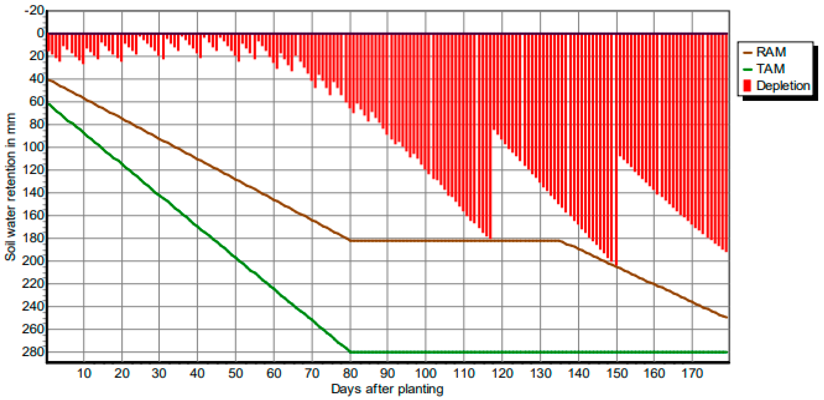
Figure 4 shows the soil water retention-growing length curve for the cotton. Figures S1–S4 show the same for the other crops. Soil water retention basically indicates the depletion of soil moisture with reference to the Total Available Water (TAW) and the existing water that the plants can extract for their growth. Growing length for a crop will give the duration of different growth stages from sowing to harvesting.

For cotton, TAW is uniform after the crop development stage, resulting in constant crop height. However, RAW is constant up to 55 days of crop growth, and after that, it will significantly fall as moisture depletion is very high. Figure 4 shows the irrigation scheduling for cotton at a fixed application depth of 100 mm and irrigation at critical moisture depletion. From Figure 4, it is clear that initially the moisture depletion level for cotton is low as a percentage of field capacity, FC, as effective rainfall almost satisfies the water demand. It increased linearly after the crop development stage, and moisture depletion was at its maximum, i.e., almost 71.4% of total available moisture (TAW), at 150 days from its showing due to less rainfall. The water deficit at the root zone increased by 7.14% within 32 days after the crop development stage, and it was again decreased by 3.6% within 30 days after the mid-season stage as the flowering stage had been reached at that time and the water requirement was comparatively low for attaining full maturity.

From Figures S1–S4, it can be observed that the moisture depletion for sugarcane is not seen in the soil water retention—crop period curve after 124 days of planting. After 49, 38, 35, and 43 days of consecutive irrigation applications, no moisture deficit was found. Here, TAW and RAW are constants throughout the planting and harvesting of the crop. Initially, the moisture depletion did not occur until 65 days after planting. Therefore, it did not affect the crop growth, but at the time of harvesting, it was low, and the variation of moisture depletion showed a marginal difference throughout the initial to mid-season stage. For maize, TAW was initially 55 mm and then increased linearly up to 180 mm, and after that, it was constant at 55 days after planting. The crop height for maize also varies between 0.3 m and a maximum of 1.0 m. Thus, a linear relationship (Figure S5) was obtained between the TAW and the crop height for maize.

h = 0.0056·TAW − 0.008

(13)

where h = crop height (m) and TAW = total available water as soil water retention (mm)—as already remarked previously.

For sorghum, irrigation started at a 50% moisture depletion level. However, with the passage of time, significant irrigation helped to achieve RAW as 80% of TAW, and this condition occurred after 90 days from the crop planting (i.e., after the mid-season stage). Here also, a linear relationship was found (Figure S6) between the crop height and TAW:

h = 0.0056·TAW − 0.0103.

(14)

For sunflowers, the maximum moisture depletion occurred 105 days after planting (i.e., 93% of TAW). From Figure S4, RAW was 45.4% of TAW, and it was then linearly varying up to the crop development stage. Then, it remained constant up to the end of the mid-season stage and was almost 50% of TAW. Then RAW achieved 78.7% of TAW at the end of the mid-season stage and up to harvesting. The following best-fit curve between the moisture depletion percentage and TAW was obtained for sunflower (Figure S7):

TAW = −0.0533·MD² + 8.099·MD − 64.436

(15)

where MD = moisture depletion percentage. The above relationships (Equations (13)–(15)) were achieved based on the simulated output obtained from CROPWAT 8.0.

3.3. Crop Characteristics

Table 4. Kurnool district: crop characteristics for cotton.

Crop Characteristics	Parameter	Unit	Observation/Value/Remark
Canopy cover	Growth of Initial Canopy	[-]	Good canopy cover
	Initial Canopy Cover (CCo)	[-]	0.32
Type of planting method: direct sowing	Canopy Size	[cm2/plant]	6.0
	Plant Density	[plants/ha]	53,333
Canopy development	Canopy Expansion	[-]	Moderate expansion
	Maximum Canopy Cover (CCx)	[%]	95
	Canopy Decline	[-]	Very slow decline
Time to reach different growth stages from sowing	Emergence	[days]	14
	Maximum Canopy	[days]	112
	Senescence	[days]	144
	Maturity	[days]	180
Flowering and yield formation	Length Building up HI	[days]	111
	Duration of Flowering	[days]	52
Time to reach flowering, maturity, and potential vegetative growth from sowing	Flowering	[days]	64
	Maturity	[days]	180
	Potential Vegetative Growth	[days]	140
Root deepening: medium rooted crop	Maximum Effective Rooting Depth	[m]	1.30
	Average Root Zone Expansion	[cm/day]	1.20
	From day 1 after Sowing to Maximum Depth	[days]	98
Crop production (no water, fertility or salinity stress)	Type of Crop	[-]	C3
	WP*	[ton/ha]	0.150
	Reference Harvest Index (HI)	[%]	35
	Biomass	[ton/ha]	9.144
	Dry Yield	[ton/ha]	2.887
	ET Water Productivity	[kg/m3]	0.73
	HI adjusted	[%]	31.6

shows different conservative and non-conservative crop parameters for cotton. Tables S9–S12 show the same for maize, sorghum, sugarcane, and sunflower, respectively, under no-water, salinity, and fertility stress.

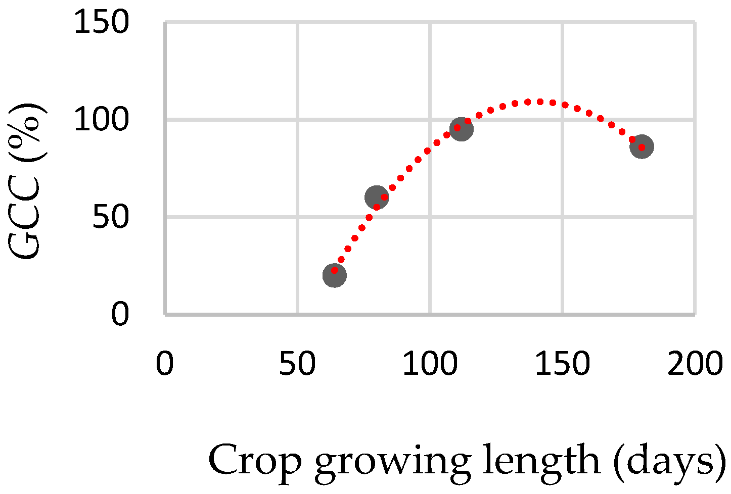
The initial canopy cover for cotton was 32% of the maximum canopy cover, and the canopy senescence occurred after 32 days from when the maximum canopy had been reached. The time taken to reach maximum canopy was 62% of the total growing period, and senescence occurred 32 days after reaching maximum canopy cover as significant moisture depletion was seen at this phase. This indicates that significant transpiration can take place throughout the entire growing cycle. The temporal growth of the cotton canopy is given by Equation (16)—with a coefficient of determination of R² = 0.99—and shown in Figure 5.

GCC = −0.0149·B² + 4.172·B − 183.34

(16)

where GCC = growth of canopy cover (%) and B is the crop growth period in days. GCC indicates the development of canopy structure, and crop growth period indicates the time taken by a crop to reach every stage of its development.

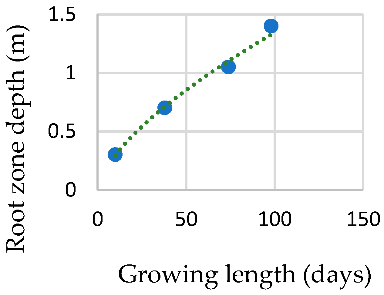
Similarly, the variation of the root zone development for cotton with the crop growth cycle (Figure 6) can be expressed as follows (R² = 0.99):

Z_r = 0.0652·B^0.657

(17)

where Z_r = root zone depth (m) and B is the crop growth period in days, as previously stated. The developed equations (i.e., Equations (16) and (17)) from Figure 5 and Figure 6, respectively, are based on the simulated crop characteristics for cotton in AQUACROP 6.1, depending on the available climatic and soil parameters.

The development of the Harvest Index (HI) with the growth period for cotton showed a gradually increasing slope with a minimum value at the start of the flowering stage and a constant value at the start of maturity (i.e., HI around 35%). Being a C3 type of crop, the slope of the curve between the biomass production and ∑Tr/ET_o is less as compared to that of C4 crops. Here, Tr is transpiration from the plant stomata. Thus, the overall yield will be low. For the given field condition, 38% of water stress was estimated during the stomatal closure and 14% at early senescence. It should be noted that we have neither used any sensors nor conducted any field experiments for the concerned crops for which water stress was calculated. The water stress coefficient was determined by using Equation (8), which is evaluated in CROPWAT 8.0 software. Moreover, we have used AQUACROP 6.1 software to calculate the yield of crops, and by default, this software would determine the water stress for different stages of crop development like canopy expansion, stomatal closure, early senescence, etc. [20]. We have not directly measured this parameter. Basically, the water stress coefficient during early senescence (K_s,sen) is responsible for the reduction of green canopy cover, whereas the same for stomatal closure (K_s,sto) plays a major role in reducing crop transpiration and root zone expansion. The target model parameters for calculating K_s,sen and K_s,sto, are green canopy cover (CC), crop transpiration coefficient (K_TR), harvest index (HI), and depth of root zone (Z_r).

Therefore, the transpiration process was affected, resulting in a lower yield for the crop. The HI is required to be adjusted by a factor that takes into account inadequate photosynthesis, pollination stress, and water stress [8]. For cotton, HI will be 2% higher in the vegetative period and 20% higher during yield formation to take into account the above-mentioned stresses. A significant amount of biomass can actually be produced as compared to potential biomass. AQUACROP 6.1 will give the value of biomass for each crop depending on crop characteristics, soil condition, cultivation operation, and climatic conditions. The biomass is calculated by using Equation (18) [8]:

$$B=WP*·\sum T_r/{ET}_0$$

(18)

where B is the biomass produced (tonne/ha), WP* is the normalised water productivity for a reference CO₂ concentration of 369.41 ppm (g/m²), T_r is the daily transpiration from plant stomata (mm), and ET₀ is the daily reference crop evapotranspiration (mm). The normalised water productivity is the slope of the curve between B and $\sum T_r/{ET}_0$.

For sugarcane, the initial canopy cover is very high, resulting in a higher leaf area index (LAI). The maximum canopy cover was developed at the crop development stage, and the crop senescence occurred 266 days after the maximum canopy cover developed. The growth of canopy cover for sugarcane is related to the crop growth period according to Equation (19), as shown in Figure S8:

GCC = −0.0034·B² + 1.4412·B − 18.672

(19)

where GCC and B are expressed in percentage and days, respectively.

The root zone expansion rate is very high for sugarcane, so the maximum crop height can be achieved within the minimum possible time after transplantation. Sugarcane is a C4-type crop. Hence, water productivity is also high. No water stress was seen during canopy expansion, stomatal closure, and early senescence, resulting in high crop production; thus, actual biomass production tends to be the same as the potential biomass. The root zone development for sugarcane shows a linear relationship with the growing period according to Equation (20), as shown in Figure S9:

Z_r = 0.0453·B + 0.2798

(20)

For maize, initial canopy cover is very high, and plant density is also very high, resulting in a higher LAI. The maximum canopy cover occurred at the end of the development stage. The duration of flowering was only 13 days, so the production of dry yield declined. The root zone development for maize shows a linear relationship with the growing period according to Equation (21) as shown in Figure S10:

Z_r = 0.0155·B + 0.3473

(21)

The water productivity for maize was high and within the range of 30–35 gm/m². The water stress was small at stomatal closure; hence, the transpiration process was not affected at the crop development stage; the water stress was comparatively high during canopy expansion. An adjusting factor of 1.01 was applied to the reference harvest index (HI_o). No adjustment was required during the vegetative period, but only an adjustment of 1% of HI_o was needed during yield formation to calculate adjusted HI. Here, the adjustment is positive. In a similar way, relationships between growth of canopy cover (GCC) versus growing days and root development versus growing period length were achieved for the other crops (e.g., sorghum and sunflower).

The above Equations (16)–(21) were achieved based on the simulated output obtained from AQUACROP 6.1.

3.4. Soil Surface Characteristics

Table 5. Soil surface characteristics of black clay soil.

Parameter	Unit	Value
TAW (FC-PWP)	[mm/m]	200
Maximum rain infiltration rate	[mm/day]	30
Maximum rooting depth	[m]	0.9
Initial soil moisture depletion (% of TAW)	[%]	50
Initial available soil moisture	[mm/m]	100

,

Table 6. Soil surface characteristics of medium (loam) soil.

Parameter	Unit	Value
TAW (FC-PWP)	[mm/m]	290
Maximum rain infiltration rate	[mm/day]	40
Maximum rooting depth	[m]	0.9
Initial soil moisture depletion (% of TAW)	[%]	0
Initial available soil moisture	[mm/m]	290

and

Table 7. Soil surface characteristics of red loamy soil.

Parameter	Unit	Value
TAW (FC-PWP)	[mm/m]	180
Maximum rain infiltration rate	[mm/day]	30
Maximum rooting depth	[m]	0.9
Initial soil moisture depletion (% of TAW)	[%]	0
Initial available soil moisture	[mm/m]	180

show different soil surface characteristics for black clay, medium (loam), and red loamy soil, respectively, as derived from CROPWAT 8.0.

Black clay soil and medium (loam) soil exhibited the highest values of TAW and the maximum rain infiltration rate. Black clay soil had an initial moisture depletion level of 50% as a percentage of TAW. Hence, cotton and sugarcane faced significant water stress problems, which could be overcome by frequent irrigation to increase the moisture content up to FC. However, medium and red loamy soil initially had no moisture depletion. So, the entire available water could be utilised by other crops.

AQUACROP 6.1 deals with (and determines) more parameters than CROPWAT 8.0, which could be more convenient for further research.

Table 8. Soil surface characteristics of black clay soil.

Parameter	Unit	Value
Thickness	[m]	1.50
TAW (FC-PWP)	[mm/m]	150
Soil Water (retention in fine soil fraction) in volume
FC	[%]	54
PWP	[%]	39
SAT	[%]	55
Hydraulic Conductivity (Ksat)	[mm/day]	35
Drainage characteristics (ζ)	[-]	0.3
Curve No. (CN)	[-]	77
Readily Evaporable Water (REW)	[mm]	14

,

Table 9. Further soil surface characteristics of medium (loam) soil.

Soil Characteristics	Soil Layer	Unit	Value
Thickness	Sandy Loam	[m]	0.5
	Loam	[m]	0.5
	Silt Loam	[m]	2.0
Total Available Water (TAW)	Sandy Loam	[mm]	120
	Loam	[mm]	160
	Silt Loam	[mm]	200
Field Capacity (FC)	Sandy Loam	[mm]	22
	Loam	[mm]	31
	Silt Loam	[mm]	33
Permanent Wilting Point (PWP)	Sandy Loam	[mm]	10
	Loam	[mm]	15
	Silt Loam	[mm]	13
Saturation Limit (SAT)	Sandy Loam	[mm]	41
	Loam	[mm]	46
	Silt Loam	[mm]	46
Hydraulic Conductivity (Ksat)	Sandy Loam	[mm/day]	1200
	Loam	[mm/day]	500
	Silt Loam	[mm/day]	575
Drainage Characteristics (ζ)	Sandy Loam	[-]	1
	Loam	[-]	0.76
	Silt Loam	[-]	0.80
Curve No. (CN)	Sandy Loam	[-]	46
	Loam	[-]
	Silt Loam	[-]
Readily Evaporable Water (REW)	Sandy Loam	[mm]	7
	Loam	[mm]
	Silt Loam	[mm]

and

Table 10. Further soil surface characteristics of red loamy soil.

Soil Characteristics	Soil Layer	Unit	Value
Thickness	Clay Loam	[m]	0.2
	Sandy Clay Loam	[m]	0.25
	Silty Clay	[m]	1.50
Total Available Water (TAW)	Clay Loam	[mm]	160
	Sandy Clay Loam	[mm]	120
	Silty Clay	[mm]	180
Field Capacity (FC)	Clay Loam	[mm]	39
	Sandy Clay Loam	[mm]	32
	Silty Clay	[mm]	50
Permanent Wilting Point (PWP)	Clay Loam	[mm]	23
	Sandy Clay Loam	[mm]	20
	Silty Clay	[mm]	32
Saturation Limit (SAT)	Clay Loam	[mm]	50
	Sandy Clay Loam	[mm]	47
	Silty Clay	[mm]	54
Hydraulic Conductivity (Ksat)	Clay Loam	[mm/day]	125
	Sandy Clay Loam	[mm/day]	225
	Silty Clay	[mm/day]	100
Drainage Characteristics (ζ)	Clay Loam	[-]	0.47
	Sandy Clay Loam	[-]	0.58
	Silty Clay	[-]	0.43
Curve No. (CN)	Clay Loam	[-]	72
	Sandy Clay Loam	[-]
	Silty Clay	[-]
Readily Evaporable Water (REW)	Clay Loam	[mm]	11
	Sandy Clay Loam	[mm]
	Silty Clay	[mm]

show the different soil surface characteristics for the above-mentioned soils from AQUACROP 6.1.

AQUACROP 6.1 underestimates TAW for black clay soil, whereas it overestimates the same for medium and red loamy soil. Hence, it could be advantageous to adopt CROPWAT 8.0 for black clay soil and AQUACROP 6.1 for medium and red loamy soil in this regard. The saturated hydraulic conductivity for black clay soil was almost equal to the maximum infiltration rate. For black clay soil, FC almost met the saturation limit; hence, readily evaporable water was very high, resulting in a higher ET_C.

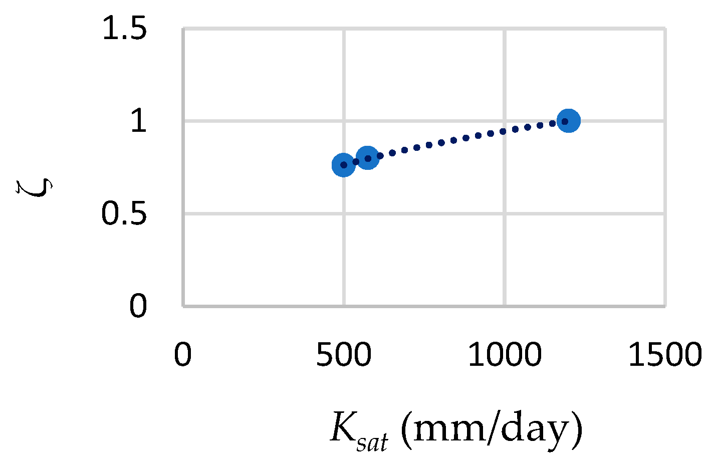
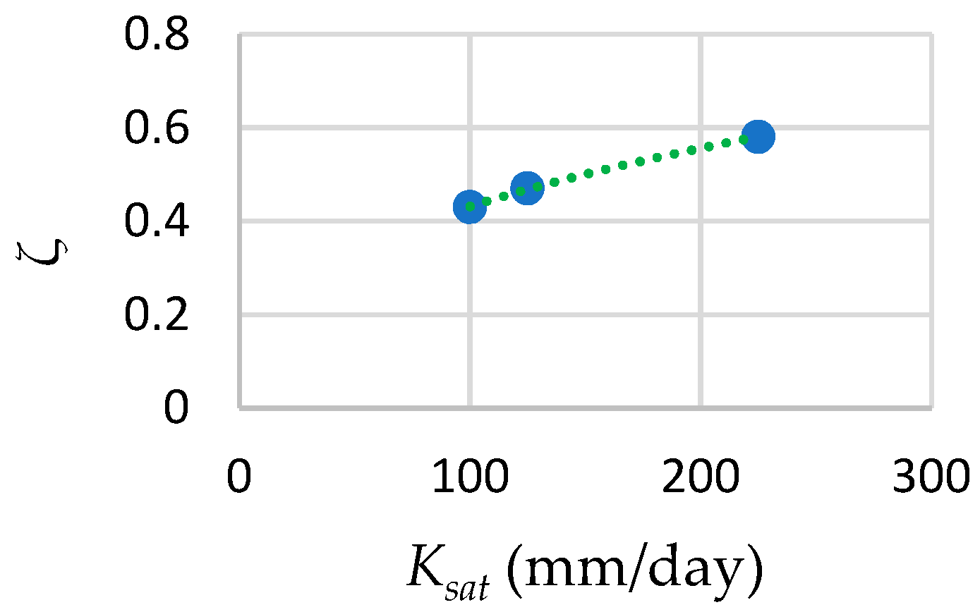
From Table 9 and Table 10, a relationship can be observed between drainage characteristics (ζ) and saturated hydraulic conductivity, expressed by Equations (22) and (23)—as shown in Figure 7 and Figure 8—for medium and red loamy soil, respectively. The variation is basically a power law with a high value of R². The developed equations (i.e., Equations (22) and (23)) from Figure 7 and Figure 8, respectively, are based on the simulated soil characteristics for medium and red loamy soil in AQUACROP 6.1, depending on the crop phenology.

ζ =0.111·K_sat^0.31

(22)

ζ = 0.0797·K_sat^0.37

(23)

where ζ expresses the fraction of drainable water day by day. For both equations, R² = 0.99. AQUACROP 6.1 also determines the Curve Number (CN) and the hydrological soil group for black clay, medium (loam), and red loamy soils. They are D, A, and C, respectively. It can be observed that for medium soil, the infiltration rate was higher as compared to the other two soils, resulting in higher percolation losses. Hence, water availability at the field could be lower, affecting the duty of the cultivated crops; thus, less area could be irrigated, though significant water supply could be carried out.

3.5. Furrow Irrigation Design Parameters

Table 11. Furrow irrigation design parameters for cotton.

Furrow Irrigation Design Parameters
Infiltration Method: Modified SCS Families
Operation Mode		Fixed Flow	Cutback Flow	Tailwater Reuse
Input parameters	Units
Flow rate	[L/s]	0.64	0.64	0.64
Length	[m]	300	300	300
Cutoff time	[min]	1920	1920	1920
Cutback ratio	[-]		0.82
Recovery ratio	[-]			0.7
Required depth	[mm]	200	200	200
Flow resistance	[s/m1/3]	0.03	0.03	0.03
Slope	[m/m]	0.02	0.02	0.02
Spacing	[m]	0.75	0.75	0.75
Maximum velocity	[m/min]	12.6	12.6	12.6
Side slope	[m/m]	1.5	1.5	1.5
Bed width	[m]	0.2	0.2	0.2
SCS		0.6	0.6	0.6
Output parameters	Units
Cutback flow	[L/s]		0.52
Advance ratio	[-]		0.23
Application efficiency	[%]	80.5	93.5	91.2
Storage efficiency	[%]	98.9	98.9	98.9
Uniformity coefficient	[%]	95.3	95.3	95.3
Distribution uniformity	[%]	86.4	86.3	86.4
Deep percolation ratio	[%]	4.2	4.9	4.3
Runoff ratio	[%]	15.2	1.6	15.2
Average applied depth	[mm]	208	208	208
Minimum infiltrated depth	[mm]	180	180	180
Maximum infiltrated depth	[mm]	218	218	218
Surface runoff	[mm]	37	3	37
Over-irrigation depth	[mm]	14	14	14
Under-irrigation depth	[mm]	9	9	9
Over-irrigation length	[m]	225	225	225
Under-irrigation length	[m]	75	75	75
Advance time	[min]	438	438	438
Depletion time	[min]	1924	1923	1924
Recession time	[min]	1951	1949	1951
Opportunity time	[min]	1513	1511	1513
No. of furrows		1	1	1

shows different furrow irrigation design parameters (e.g., application efficiency, storage efficiency, cut-off time, advance time, recession time, furrow length, surface runoff ratio, and deep percolation ratio) by taking into account different input parameters (e.g., flow rate, furrow cross-section) for cotton. The FURDEV model calculates the values of uniformity coefficient (UC), distribution uniformity (DU), deep percolation ratio, and surface runoff ratio for furrow irrigation based on input parameters like flow rate, furrow cross sections, and soil infiltration characteristics for the crop under consideration. These above-mentioned parameters have been determined by using Equations (24)–(27) [19,24].

$$\mathrm{Uniformity}\mathrm{Coefficient}UC=1-\sum \left(\frac{\left|D_i-D_{avg}\right|}{n·D_{avg}}\right)$$

(24)

$$\mathrm{Distribution}\mathrm{Uniformity}DU=\frac{D_{min}}{D_{avg}}$$

(25)

$$\mathrm{Deep}\mathrm{Percolation}\mathrm{Ratio}DPR=\frac{D_{dp}}{D_a}$$

(26)

$$\mathrm{Surface}\mathrm{Runoff}\mathrm{Ratio}SRR=\frac{D_{sr}}{D_a}$$

(27)

where D_i is the depth of water in the furrow for ith emitter (mm); D_avg is the average infiltrated depth (mm); n is the number of emitters along the length of the furrow; D_min is the minimum infiltrated depth (mm); D_dp is the deep percolation depth (mm); and D_sr is the surface runoff depth (mm), which is the difference between the actual infiltrated depth (D_a) and the average infiltrated depth (mm) (i.e., D_sr = D_a − D_avg). Tables S13–S15 show the same for maize, sorghum, and sunflower.

The programme FURDEV clearly shows the impact of different furrow irrigation design parameters on the yield of crops as well as the proper management of irrigation water with the help of AQUACROP 6.1. Among all the three forms of operation modes, the cutback flow method and tailwater reuse method were found to be more convenient because the application efficiency and storage efficiency were relatively higher as compared to the fixed flow method for the same flow rate, soil infiltration characteristics, and furrow cross sections [19]. However, the under-irrigation depth and over-irrigation depth were almost the same in these three modes.

From Table 11, it was observed that cotton has a less advanced ratio, requiring more uniformity in irrigation. A significant amount of water can be utilised from the tail end of the field as the recovery ratio is relatively high, which ensures an economical and controlled use of water. Cotton has a very short depletion phase and a long ponding phase, indicating that the rate of decrease in surface water storage was low and the availability of irrigation water in the field was high for a long period of time. Due to the long ponding phase, the depth of water in the field increased, resulting in a lower moisture deficit. Cutback flow mode was more convenient for cotton as surface runoff depth was low. More water can be used to increase the water content in the soil moisture zone. Application efficiency increases by 16.14% and 13.3% for cutback flow and tailwater reuse methods compared to fixed flow methods, respectively. Whereas distribution uniformity and uniformity coefficient were independent of furrow length and flow rate for cotton. Over irrigation depth was slightly higher as compared to under irrigation depth for cotton, maize, and sunflower, except for sorghum. Additionally, it was higher when the fixed flow method was used. Therefore, the other two modes of operation could be beneficial for obtaining the maximum possible efficiency. More controlled water application may be possible for maize with the lowest cutback ratio. However, for maize, surface runoff depths were comparatively higher, and they were higher for the tailwater reuse method for all the crops. Whereas the cutback flow method simulates a very small amount of surface runoff for all the crops with the same input parameters. A reverse curve was obtained between the relationship between flow rate and application efficiency for the crops for cutback flow and tailwater reuse methods.

From Table 11 and Tables S9–S12, one can observe: (i) spacing of furrows, gradient, surface roughness, and furrow cross sections had no influence on the furrow length, flow rate, cutoff time, application efficiency, storage efficiency, and many other design parameters; rather, they depended upon crop type; (ii) a larger furrow length would result in a larger distribution uniformity and uniformity coefficient. Hence, more uniformity in irrigation could be obtained. In this regard, sunflower had the minimum Distribution Uniformity (DU) and Uniformity Coefficient (UC) and maize had the maximum UC and DU; and (iii) surface runoff ratio increased with increasing furrow length except for sunflower. A lower flow rate will give a higher deep percolation ratio for all the crops as the applied water depth on the field will be less, resulting in the development of significant lengths of under irrigation, which clearly signifies the occurrence of water stress and lower application efficiency.

Application efficiency increases with increasing the furrow length for sunflower, cotton, and sorghum, but storage efficiency is almost independent of furrow length. Lower furrow length gives lower application efficiency, resulting in a more non-uniform water application. Additionally, improper water distribution does not satisfy the crop’s water demand. The distribution uniformity (DU) and uniformity coefficient (UC) are independent from the flow rate, furrow length, and operation mode for all the crops. The average infiltration opportunity time for cotton, maize, sunflower, and sorghum is calculated as 1513 min, 1093 min, 794 min, and 1027 min, respectively. So, more non-uniformity in irrigation operations has been seen for cotton, which has a large opportunity time.

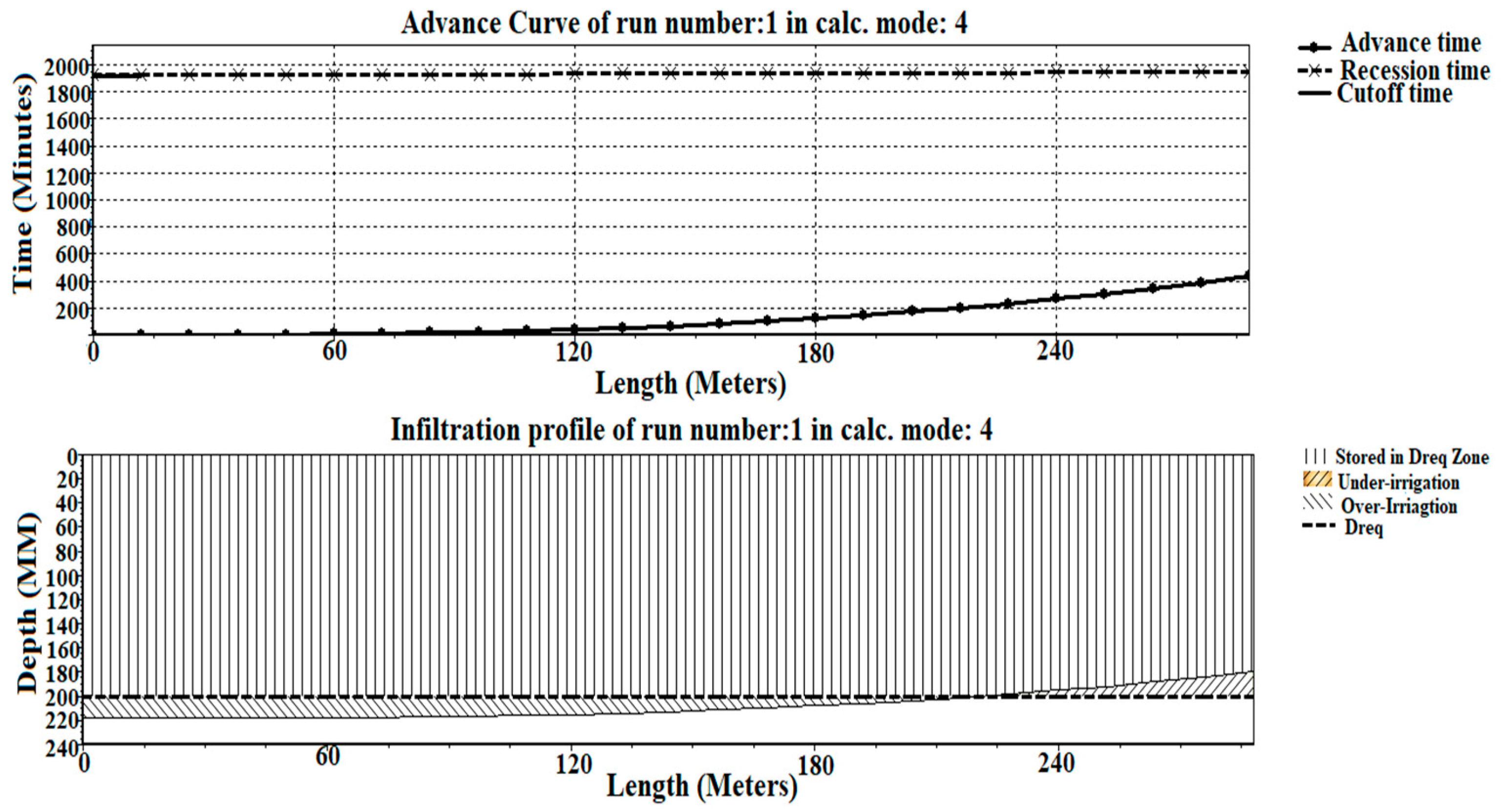
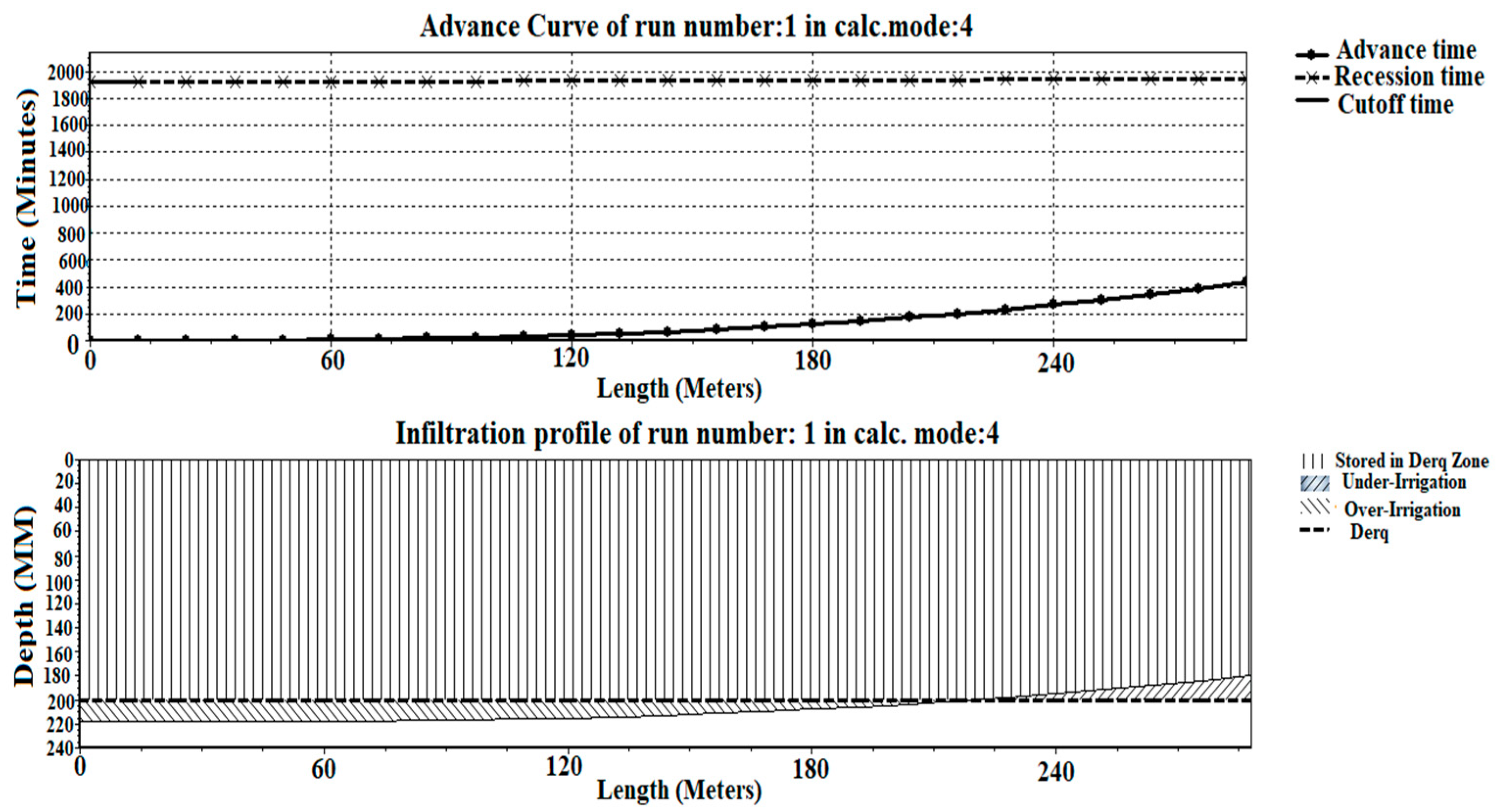
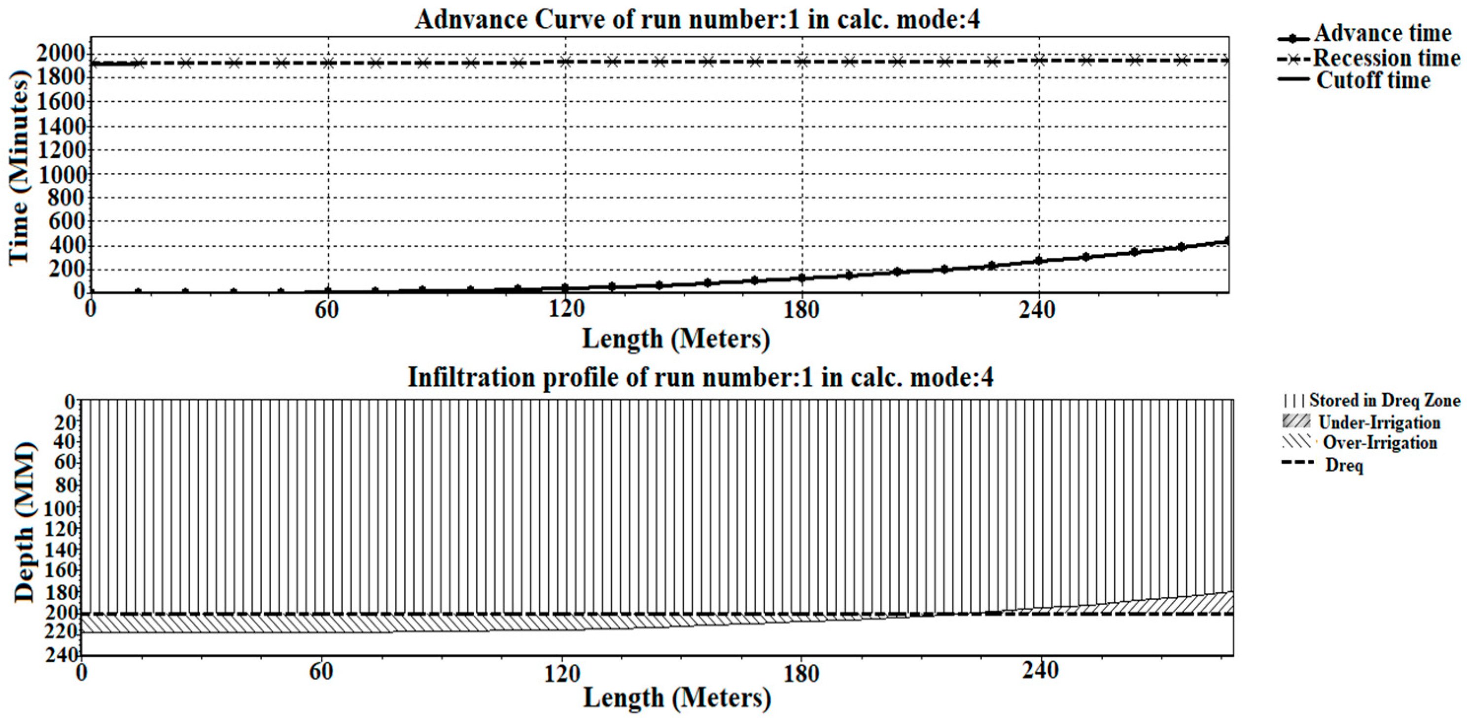
Additionally, by using the results of FURDEV, the advance curve and the irrigation profile were prepared. Figure 9, Figure 10 and Figure 11 show the advance curve and the irrigation profile for the cotton for three different modes of operation. In a similar way, the same profiles were obtained for the remaining crops and shown in Figures S11–S19 under the same modes of operation. The advance curve shows the variation of different hydraulic phases of furrow irrigation with furrow length and gives the value of infiltration opportunity time, which is the difference between advance time and recession time. It will signify uniformity in irrigation operations, whereas the irrigation profile shows different water depths in the field along the furrow length, which further indicates whether there is any possibility of waterlogging due to over-irrigation, surface runoff loss, or the occurrence of water stress [19].

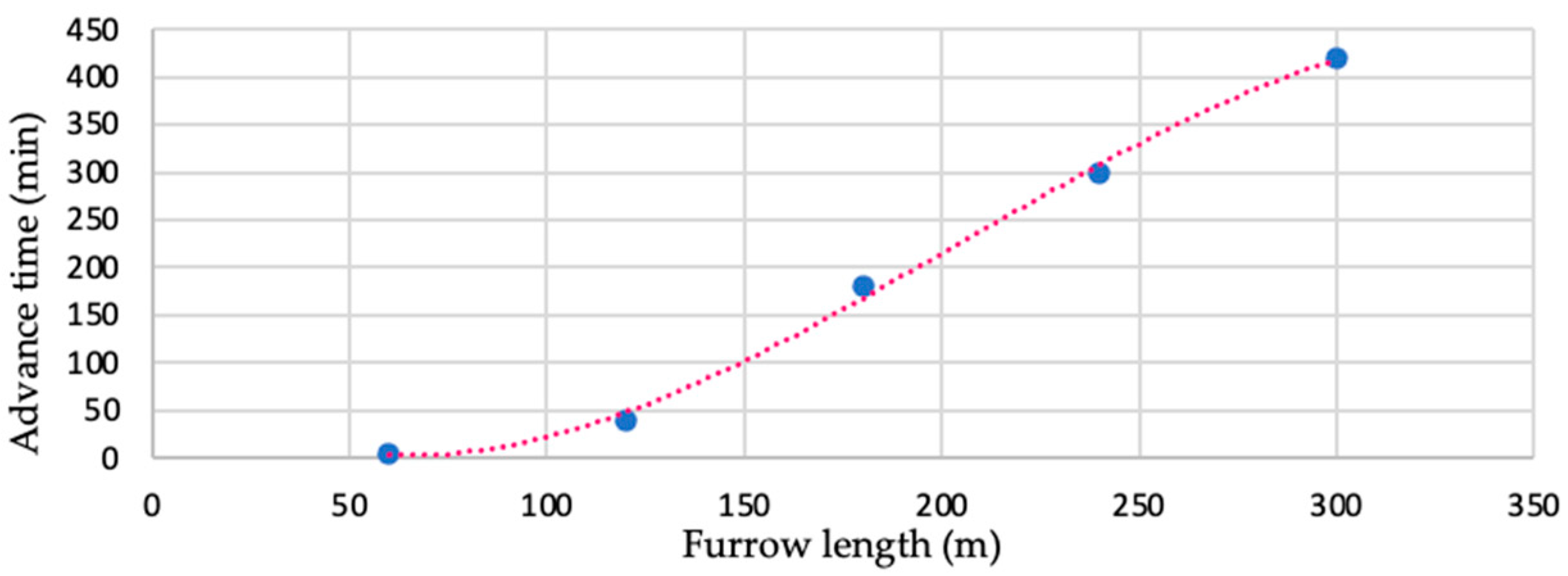
From the advance curve, it can be observed that cotton has the highest opportunity time while sunflower has the lowest one. Maize and sorghum have almost the same opportunity time, indicating that more uniformity in the irrigation operation will ensure more infiltration depth through the soil. From the advance curve, it can be observed that the advance time gradually increases with increasing the furrow length for all the crops under all the modes of operation. In the case of cotton, a relationship (with R² = 0.997) can be established between the advance time and the furrow length as follows (Figure 12). The relationship was established based on the simulated output obtained from FURDEV and the curve of best fit.

T_a = −4·10⁻⁵L³ + 0.0249L² − 2.6964L + 84

(28)

where T_a is the advance time (min) and L is the length of the furrow (m).

Analogously, the advance curve for sorghum (Figure S20) can be expressed by Equation (29). This relationship was established based on the simulated output obtained from FURDEV and the curve of best fit:

T_a = 0.0012L² − 0.0789L − 5

(29)

Similar relationships can be obtained for the remaining crops. More advance time will ensure that the water takes a long time to reach the downstream end of the field until the inflow has been started; therefore, more infiltration loss and deep percolation loss will occur. Subsequently, the application’s efficiency will decrease. Whereas the furrow length has no influence on the recession curve, 83.4% of the total furrow length will consume maximum over-irrigation length for maize and 58.42% of the total furrow length will consume minimum over-irrigation length for sorghum. This clearly indicates that a significant portion of over-irrigation length would occur, resulting in deeper percolation loss and surface runoff loss for the crops.

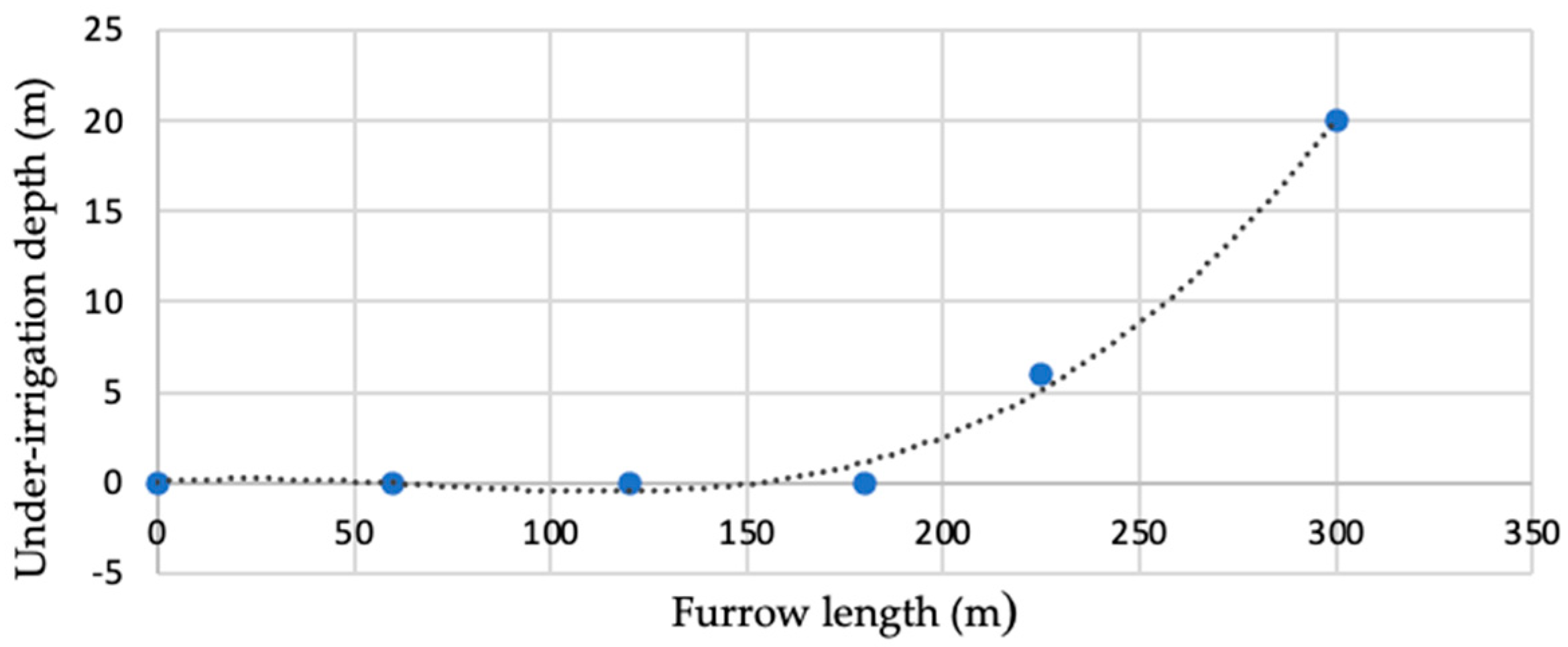
Figure 13 shows that a polynomial relationship can be obtained between the under-irrigation depth and the furrow length for cotton (Equation (30)). The relationship was established based on the simulated output obtained from FURDEV and the curve of best fit (with R² = 0.993):

D_u = 2·10⁻⁶L³ − 0.0004L²+ 0.015L + 0.0537

(30)

where D_u = under-irrigation depth (mm) and L = length of the furrow (m). Similar relationships were achieved for the other crops.

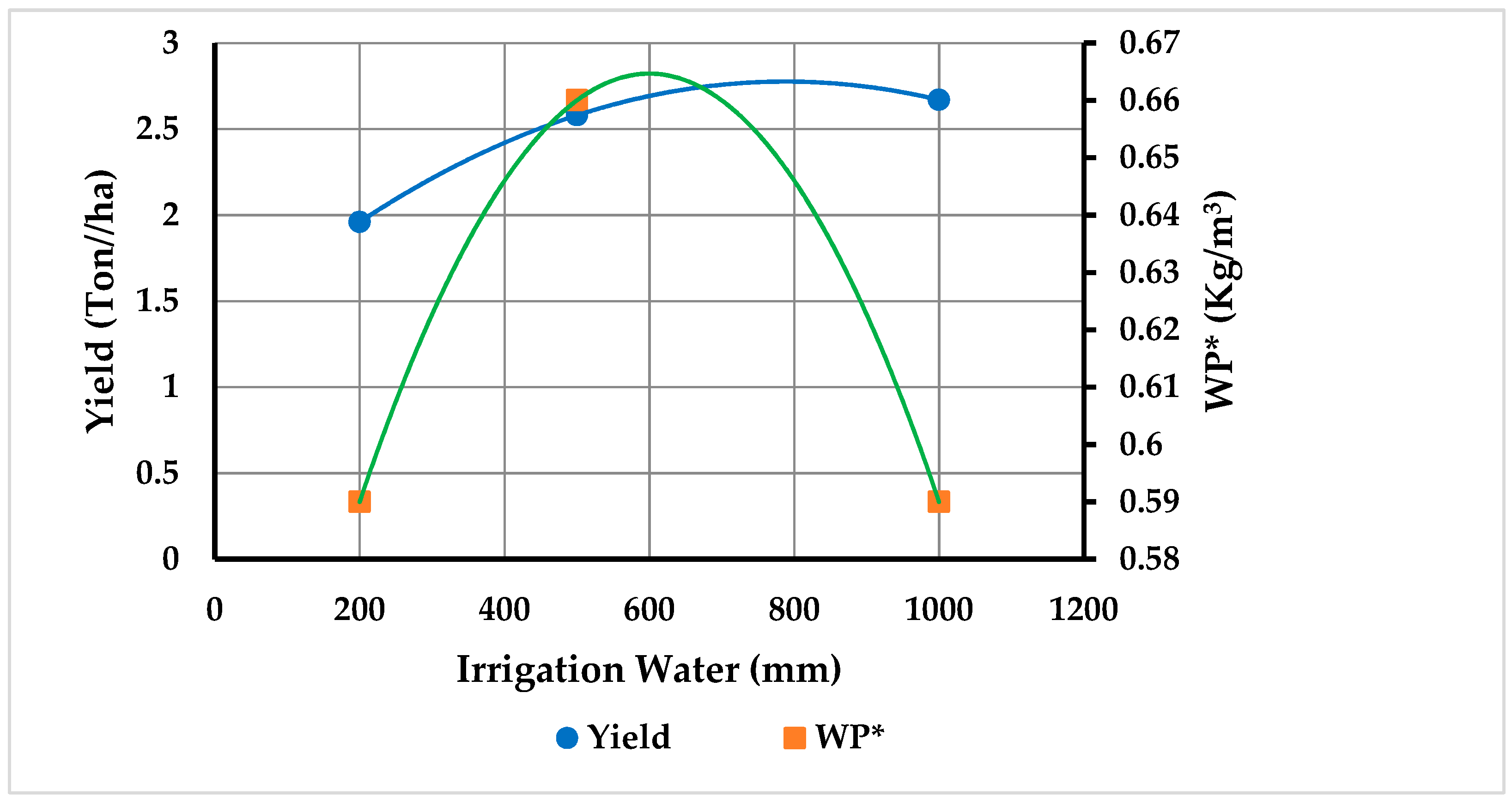
Figure 14 shows the crop productivity depending on the irrigation water for cotton. Similarly, Figures S21 and S22 show the same for maize and sunflower, respectively.

The crop productivity-irrigation water relationship (Figure 14, Figures S21 and S22) for cotton, maize, and sunflower can be established from the output obtained from AQUACROP 6.1.

Initially, for cotton, the water productivity (WP) was small, and it increased with decreasing water application. Similarly, the dry yield for cotton decreased from 2.6 tonne/ha to 1.68 tonne/ha at a decreasing water depth from 1000 mm to 200 mm. It was noted that there was a significant reduction in the irrigation water requirement of 80%, with a reduction in the ET water productivity of 10.6%.

Similarly, for maize, the optimum depth of water application was 275 mm and the maximum WP was 2.4 kg/m³; dry yield linearly increased with increasing the irrigation water. The highest yield was obtained at a water depth of 770 mm. Figure S21 shows a reduction in the irrigation water requirement of 85.7% with a reduction in the ET water productivity of 7.76%. Similarly, Figure S22 shows a reduction in the irrigation water requirement of 50% with a reduction in the ET water productivity of 1.45% for sunflower. These results clearly highlight the need for controlled water management for irrigation to optimize the beneficial use of water.

4. Discussion

From the literature review, it can be concluded that previously there was no work to estimate irrigation water demand, different conservative and non-conservative crop parameters, and furrow irrigation design parameters for Kurnool district, Andhra Pradesh. Proper assessment of water consumption, irrigation application, and irrigation timing for cotton, sugarcane, sorghum, sunflower, and sugarcane is important for Kurnool district as suitable soil and environmental conditions are available to cultivate these crops. To enhance the productivity of these crops in an economical manner, proper knowledge of local climatic conditions, field management conditions, irrigation methods, and the utilisation of available water resources in a controlled manner is very important for planning and designing efficient irrigation systems.

In this present study, the dependency of evapotranspiration on climatic and meteorological factors and the variation of K_c with different growth stages of these crops are examined. Later, the irrigation water needed for these crops was calculated, and the contribution of effective rainfall was also studied. The irrigation schedule for most of the crops was observed by adopting irrigation at critical depletion and refilling soil at field capacity so as to reduce the yield response factor and get optimum water productivity. To enhance the productivity of these crops, a comprehensive study was carried out to observe different crop characteristics and their temporal variation with crop growing periods. Soil surface characteristics play a major role in estimating water use efficiency for furrow irrigation systems. Infiltration opportunity time, cutback ratio, advance ratio, tailwater reuse ratio, and surface runoff ratio were estimated by using three different modes of irrigation. These are some important parameters of furrow irrigation that indicate a higher efficiency of water use with a high application efficiency and uniformity coefficient.

5. Conclusions

The evaluation of the crop water requirement (CWR) and irrigation scheduling for cotton, sugarcane, sorghum, maize, and sunflower was investigated in this study. Different important crop characteristics, soil characteristics, and surface irrigation parameters were simulated using different approaches. A strong connection between these parameters was also discussed comprehensively. FAO CROPWAT 8.0 is a very important platform for the proper assessment of evapotranspiration, crop water requirements, and irrigation scheduling. Furthermore, the AQUACROP 6.1 and FURDEV models are useful for the accurate study of crop characteristics and furrow irrigation design parameters, respectively.

Reference crop evapotranspiration was higher in the dry summer season, and effective rainfall provided a small contribution, mainly for sorghum and sunflower. Crop water requirements follow a descending order, as follows: CWR sugarcane > CWR sunflower > CWR cotton > CWR maize > CWR sorghum.

The gross irrigation requirement for all the crops has been obtained by adopting an application efficiency of 70%. NIR was determined as 200 mm, 1423.2 mm, 220 mm, 150 mm, and 150 mm for cotton, sugarcane, maize, sorghum, and sunflower, respectively. CROPWAT 8.0 also shows variation of crop height with TAW, and AQUACROP 6.1 establishes a relationship between different crop phenology and their growing length. The maximum dry yield obtained for maize was 13.586 tonne/ha. Additionally, different soil surface characteristics were obtained and compared by CROPWAT 8.0 and AQUACROP 6.1 for checking model performance. The FURDEV model estimated economical furrow length, and it increases with an increase in the flow rate for all the crops except sunflower. Along with that, different furrow irrigation design parameters were evaluated and their effect on irrigation operations properly studied.

By using crop water requirements and irrigation scheduling for different crops, irrigation schemes and cropping patterns can be studied in the future. The proposed approach can be used to determine different types of water consumption in a particular month or day, which can be further processed to estimate the area to be cultivated for these crops.

Along with that, the impact of different field management methods for irrigation can be obtained on biomass production, soil fertility, and weed management so that an engineer may design proper irrigation systems and methods to use available water resources with high accuracy and the desired quality.

References

1. Veeranna, J.; Mishra, A.K. Estimation of evapotranspiration and irrigation scheduling of Lentil (Lens Culinaris) using CROPWAT 8.0 Model for Anantapur district, Andhra Pradesh, India. J. AgriSearch 2017, 4, 255–258. [Google Scholar] [CrossRef]
2. Ratna Raju, C.; Yella Reddy, K.; Satyanarayana, T.V.; Yogitha, P. Estimation of crop water requirement using CROPWAT software in Appapuram channel command under Krishna western delta. Int. J. Agric. Sci. 2016, 8, 1644–1649. [Google Scholar]
3. Reddy, A.G.S. Water level variations in fractured, semi-confined aquifers of Anantapur district, southern India. J. Geol. Soc. India 2012, 80, 111–118. [Google Scholar] [CrossRef]
4. Babu, R.G.; Veeranna, J.; Kumar, K.N.R.; Rao, I.B. Estimation of water requirement for different crops using CROPWAT model in Anantapur region. Asian J. Environ. Sci. 2014, 9, 75–79. [Google Scholar] [CrossRef]
5. Ewaid, S.H.; Abed, S.A.; Al-Ansari, N. Crop water requirements and irrigation schedules for some major crops in Southern Iraq. Water 2019, 11, 756. [Google Scholar] [CrossRef]
6. Naik, B.R. Optimal crop water requirement for Araniar reservoir basin. Int. Res. J. Eng. Technol. 2016, 3, 2161–2165. [Google Scholar]
7. Er-Raki, S.; Chehbouni, A.; Ezzahar, J.; Khabba, S.; Lakhal, E.K.; Duchemin, B. Derived crop coefficients for winter wheat using different reference evpotranspiration estimates methods. J. Agric. Sci. Technol. 2011, 13, 209–221. [Google Scholar]
8. Steduto, P.; Raes, D.; Hsiao, T.C.; Fereres, E.; Heng, L.; Izzi, G.; Hoogeveen, J. AquaCrop: A new model for crop prediction under water deficit conditions. Drought Manag. Sci. Technol. Innov. 2009, 33, 285–292. [Google Scholar]
9. Parvathi, K.S.; Shubha Lakshmi, B.S.; Arjun, K.; Shivakumar, B.P. A study on crop water requirement from the Manual Method. Glob. J. Eng. Sci. Res. 2017, 4, 80–84. [Google Scholar]
10. Hou, L.; Wenninger, J.; Shen, J.; Zhou, Y.; Bao, H.; Liu, H. Assessing crop coefficients for Zea mays in the semi-arid Hailiutu River catchment, northwest China. Agric. Water Manag. 2014, 140, 37–47. [Google Scholar] [CrossRef]
11. Aghdasi, F. Crop Water Requirement Assessment and Annual Planning of Water Allocation; International Institute for Geo-Information Science and Earth Observation: Enschede, The Netherlands, 2010. [Google Scholar]
12. Parwin, R. A study on the crop water requirement for agriculture in a typical river basin of India. Int. J. Water Res. 2014, 2, 67–70. [Google Scholar]
13. Egbuikwem, P.N.; Obiechefu, G.C. Evaluation of evapotranspiration models for waterleaf crop using data from lysimeter. In Proceedings of the 2017 ASABE Annual International Meeting, Spokane, DC, USA, 16–19 July 2017. [Google Scholar]
14. Allen, R.G.; Pereira, L.S.; Raes, D.; Smith, M. Crop Evapotranspiration—Guidelines for Computing Crop Water Requirements—FAO Irrigation and Drainage Paper 56; FAO—Food and Agriculture Organization of the United Nations: Rome, Italy, 1998. [Google Scholar]
15. Yigezu, T.T.; Narayanan, K.; Hordof, T. Effect of furrow length and flow rate on irrigation performances and yield of maize. Int. J. Eng. Res. Technol. 2016, 5, 602–607. [Google Scholar]
16. Michael, A.M.; Mohan, S.; Swaminathan, K.R. Design and Evaluation of Irrigation Methods; Water Technology Centre, Indian Agricultural Research Institute: New Delhi, India, 1972. [Google Scholar]
17. Kore, G.G. Effect of furrow irrigation technical parameters on field application performances of short furrow and yield of onion crop in Bako, Ethiopia. Int. J. Eng. Res. Technol. 2020, 9, 1692–1698. [Google Scholar]
18. Adamala, S.; Raghuwanshi, N.S.; Mishra, A. Development of surface irrigation systems design and evaluation software (SIDES). Comput. Electron. Agric. 2014, 100, 100–109. [Google Scholar] [CrossRef]
19. Jurriëns, M.; Zerihun, D.; Boonstra, J.; Feyen, J. SURDEV: Surface Irrigation Software (Design, Operation, and Evaluation of Basin, Border, and Furrow Irrigation; Alterra-ILRI: Wageningen, The Netherlands, 2001. [Google Scholar]
20. Doorenbos, J.; Kassam, A.H. Yield response to water. Irrig. Drain. Pap. 1979, 33, 257. [Google Scholar]
21. Surendran, U.; Sushanth, C.M.; Mammen, G.; Joseph, E.J. Modelling the crop water requirement using FAO-CROPWAT and assessment of water resources for sustainable water resource management: A case study in Palakkad district of humid tropical Kerala, India. Aquat. Procedia 2015, 4, 1211–1219. [Google Scholar] [CrossRef]
22. Tibebe, M.; Zemadim, B. Water demand analysis and irrigation requirement for major crops at Holetta catchment, Awash subbasin, Ethiopia. J. Nat. Sci. 2015, 5, 117–128. [Google Scholar]
23. Alemayehu, Y.A.; Steyn, J.M.; Annandale, J.G. FAO-type crop factor determination for irrigation scheduling of hot pepper (Capsicum annuum L.) cultivars. S. Afr. J. Plant Soil 2009, 26, 186–194. [Google Scholar] [CrossRef]
24. Waqas, M.S.; Cheema, M.J.M.; Hussain, S.; Ullah, M.K.; Iqbal, M.M. Delayed irrigation: An approach to enhance crop water productivity and to investigate its effects on potato yield and growth parameters. Agric. Water Manag. 2021, 245, 106576. [Google Scholar] [CrossRef]
25. Tewabe, D.; Abebe, A.; Tsige, A.; Enyew, A.; Worku, M. Determination of crop water requirements and irrigation scheduling of wheat using CROPWAT at Koga and Rib irrigation scheme, Ethiopia. Indian J. Ecol. 2022, 49, 363–371. [Google Scholar]
26. Aydın, Y. Quantification of water requirement of some major crops under semi-arid climate in Turkey. PeerJ 2022, 10, e13696. [Google Scholar] [CrossRef] [PubMed]
27. Ahmadi, S.H.; Jorenush, M.H.; Boroomand Nasab, S. Regional modeling of winter wheat yield and water productivity under water-saving irrigation scenarios. J. Water Clim. 2022, 13, 3547–3565. [Google Scholar] [CrossRef]
28. Solgi, S.; Ahmadi, S.H.; Sepaskhah, A.R.; Edalat, M. Wheat yield modeling under water-saving irrigation and climatic scenarios in transition from surface to sprinkler irrigation systems. J. Hydrol. 2022, 612, 128053. [Google Scholar] [CrossRef]
Figure 1. Location map of Kurnool District in India.
Water 15 01801 g001
Figure 2. Monthly variation in weather station parameters and reference crop evapotranspiration for Kurnool district in 2005.
Water 15 01801 g002
Figure 3. Monthly variation in rainfall and effective rainfall for Kurnool district in 2005.
Water 15 01801 g003
Figure 4. Soil water retention–growing length curve for cotton. In red depletion, brown RAW, and green TAW.
Water 15 01801 g004
Figure 5. Variation of canopy cover growth with the crop growing period length for cotton.
Water 15 01801 g005
Figure 6. Variation of root development with the crop’s growing length for cotton.
Water 15 01801 g006
Figure 7. Drainage characteristics curve for medium (loam) soil.
Water 15 01801 g007
Figure 8. Drainage characteristics curve for red loamy soil.
Water 15 01801 g008
Figure 9. Advance curve and irrigation profile for cotton in the fixed flow method.
Water 15 01801 g009
Figure 10. Advance curve and irrigation profile for cotton in the cutback flow method.
Water 15 01801 g010
Figure 11. Advance curve and irrigation profile for cotton in the tail water reuse method.
Water 15 01801 g011
Figure 12. Variation of the advance curve with furrow length for cotton.
Water 15 01801 g012
Figure 13. Variation of the under–irrigation depth with furrow length for cotton.
Water 15 01801 g013
Figure 14. Crop productivity–irrigation water relationship for cotton.
Water 15 01801 g014