Effectiveness of Controlled Tile Drainage in Reducing Outflow and Nitrogen at the Scale of the Drainage System

Abstract

The impact of controlled drainage (CD) on the groundwater table (GWT), drainage outflow, surface runoff, and nitrogen reduction at the drainage system scale in the Wielkopolska region was analyzed in this study. Based on field research, mainly by monitoring of GWT changes in 2019–2020, the DRAINMOD model was calibrated and validated. Hydrological soil water balance simulations were carried out with 36 and 9 combinations for CD and free drainage (FD), respectively. The modelling period was March-September for 10 different dry, wet, and normal years from the period of 1961 to 2020. The next step was to use the results of drainage outflow modelling and chemical constituent analyses of drainage water samples to determine NO₃-N concentrations and calculate NO₃-N pollution loads. As a result of the simulations, the importance of the timing of the start of the outflow retention in the adopted model variants was determined, indicating the earliest assumed date of 1 March. The appropriate CD start date as well as the initial GWT has a significant impact on the effectiveness of CD application in reducing the volume of drainage outflow and reducing the amount of NO₃-N entering open water with it. The application of CD under the conditions of the analyzed drainage facility makes it possible to retain up to 22 kg of NO₃-N per hectare.

1. Introduction

Agriculture is the main diffuse source of both surface water and groundwater pollution, such as nutrients, pesticides or pharmaceuticals, in many European countries [1]. One of the factors affecting excess nutrients in soil and water pollution is the excessive use of fertilizers for plant production derived from mineral and organic fertilizers [2,3,4]. Nutrients enter the water cycle through erosion, surface runoff, leaching, or inflow from the contaminated discharge of sewage and groundwater into surface waters. The presence of too many nutrients affects water quality and human health [5,6,7,8,9,10].

Legislative action within the member states of the European Union, the implementation of the Water Framework Directive (WFD) [11], the Nitrates Directive [12], or the Sustainable Use of Pesticides Directive [13] by the Baltic member states is still not effective. These directives specify that the key to achieving good environmental status in marine waters is good water quality in the rivers that flow into the sea. They provide a framework for the protection of inland, transitional, and coastal waters. The objective was to ensure good surface water and groundwater status by 2015 or, in exceptional cases, by 2021 or 2027. Furthermore, the directives require the adoption of measures to ensure that farmers with agricultural land that causes or is likely to cause the nitrate pollution of waterways meet minimum requirements for the use of nitrogen fertilizers. The strategy to improve the condition of the Baltic Sea involves regional cooperation to create a series of recommendations for farmers to reduce nutrient inputs [14,15,16]. According to the Second Report of European Waters, river basin management plans (RBMPs) particularly those involving agriculture, indicate that significant pressures result from pollution from diffuse and point sources. Diffuse water pollution from agriculture (DWPA) was found to affect 22% of the surface water bodies and 28% of the groundwater area, leading to the deterioration of good ecological and chemical status. Point sources are agricultural subsurface drainage systems, and are also known as field, free, or conventional drainage associated with agricultural activities [17].

Non-irrigated agriculture is struggling to cope with more frequent and prolonged extreme events, such as droughts, in various aspects: meteorological, hydrological, agricultural, and socio-economic. The last concerns a water shortfall in relation to the anthropogenic supply and demand in the socio-economic system. Drought is one of the most severe natural hazards, and is also a natural event that occurs in all climates [18,19]. Between 2018 and 2020, Europe experienced a drought of unprecedented intensity that persisted for more than two years. It affected a large part of the continent, with an average surface coverage of 35.6% and an average duration of 12.2 months [20]. Drought in Polish agriculture usually occurred every five years, until recently, when it began to affect significant areas of the country almost every year since 2015 [21]. The economic costs caused by the occurrence of water shortages are losses in agricultural production, so it has become necessary to provide state aid to the affected farmers. In 2015, this amounted to about PLN 500 million; however, in 2018 it was already four times more than this, at just over PLN 2 billion [22].

The agricultural sector is under pressure from a rapidly growing human population affecting the intensification of agricultural production, both plant and animal. Human economic activity and progressive urbanization have a negative impact on water quality. As a result of global climate change, the climate will become drier in some regions, wetter in others, and all areas will be more variable and unpredictable [23,24]. Thus, water-dependent agricultural areas will experience greater water scarcity, while others will become wetter. However, without adaptation to these changes, even regions with relatively smooth projected changes could consequently experience losses in agricultural forage and folder production [25]. The increase in these losses is related to the growing incidence and intensity of agricultural and hydrological droughts in response to rising evapotranspiration and runoff with relatively constant precipitation [26,27,28]. Hence, agricultural and water policies require accurate information on the impact of climate change on available water resources [29]. A simplified water accounting framework can be fully sufficient to synthesize basin-level information on climate change effects [29] and adaptation measures for the effective planning and management of agricultural water resources [26]. Progressive climate change will require the selection of appropriate crops, as well as the optimization of water management through existing drainage and irrigation systems, among other things [30]. A tile drainage system at field scale is a potential component of agricultural adaptation to climate change. The net effect on the water supply is open to question, but in this case, regions that become drier will experience transition and frictional costs. Referring to data from the year 2000, the variation in the average value of irrigated water, taking into account the variation between crops in different regions, was found to range from 0.09 USD/m³ in South Asia to 0.42 USD/m³ in Europe [31].

Poland is one of the member states of the European Union. According to accepted standards, the maximum permissible concentration of nitrate nitrogen in water intended for consumption according to the regulations in force is 50 mg/L of NO₃ (about 11.3 mg/L of NO₃-N), while the recommended value is 25 mg/L of NO₃. These values are recommended by the World Health Organization (WHO) [32,33]. Concentrations of nitrogen compounds in surface waters are important from the point of view of implementing the WFD and achieving good water status. In natural watercourses, average annual concentrations of ammonia nitrogen should not exceed 0.4 mg/L of NH₄-N, nitrate nitrogen should not exceed 2.0 mg/L of NO₃-N, and total nitrogen should not exceed 3.3 mg/L of N [34]. In Poland, the problem of high nutrient pollution is particularly relevant for lowland rivers in intensively farmed areas. Lowland rivers are usually polluted by a large catchment area, and even with a good wastewater treatment system and good agricultural practices, some nutrients reach the waters and pose a threat to their quality [35,36,37,38]. According to Janicka et al. [39] the Głuszynka River located in a river and lake system located in a lowland area showed variability in N content, from 0.87 to 9.32 mg/L of N and 0.07–6.95 mg/L of NO₃-N over three years. Fedorczyk et al. [40] reported the average concentration during the growing season of 2019 at the level of 3.4 mg/L for the catchment area of the Glinianka inflow, characterized by a predominant share of arable land (70%) during the recorded drought.

Currently, many countries around the world are increasingly taking action to reduce the loss and recirculation of nutrients to surface waters, slow down the runoff of water, and thus store it [41,42]. The role of subsurface drainage is changing from a single-purpose measure to an important component of an integrated land use drainage and/or irrigation system [43]. The implementation and testing of drainage mitigation measures is becoming a sought-after solution for climate change mitigation and water access in agricultural production. One type of drainage mitigation measures is CD, also known as controlled tile drainage (CTD), which is a part of the drainage water management practices that are increasingly being used in many other countries [41,44,45].

A number of studies on CD have shown that it is very effective in reducing the export of nutrients such as nitrogen and phosphorus in drainage outflows, thereby providing significant environmental benefits [46,47,48,49]. In addition, there are studies identifying the positive effects of CD on crop yields and their economic benefits [44,50,51,52,53]. However, some studies have found no significant effects of CD [47,54], and in a few cases they have found negative effects, such as a reported decrease in average crop yields [55,56]. Significant differences in the performance of this practice depend on weather conditions such as the amount and timing of rainfall and the management strategy adopted for each year [44]. In addition to experimental field studies, modelling tests are performed for CD application under different spatial, soil and groundwater conditions prior to the installation of equipment. Simulations of field hydrology are carried out for various future climate scenarios of CD application in south-eastern Sweden, central-western Poland, and Ohio, USA [30,57,58].

The aim of this study is to evaluate the impact of CD in comparison to FD practice on the reduction of water outflow from the drainage object in quantitative and qualitative aspects by combining the simulation of hydrological modeling and the results of field measurement. The analyses provide useful information for assessing the impact of drainage management on hydrology and environmental problems related to water and nitrogen at the scale of the drainage system.

2. Materials and Methods

2.1. Study Area Description

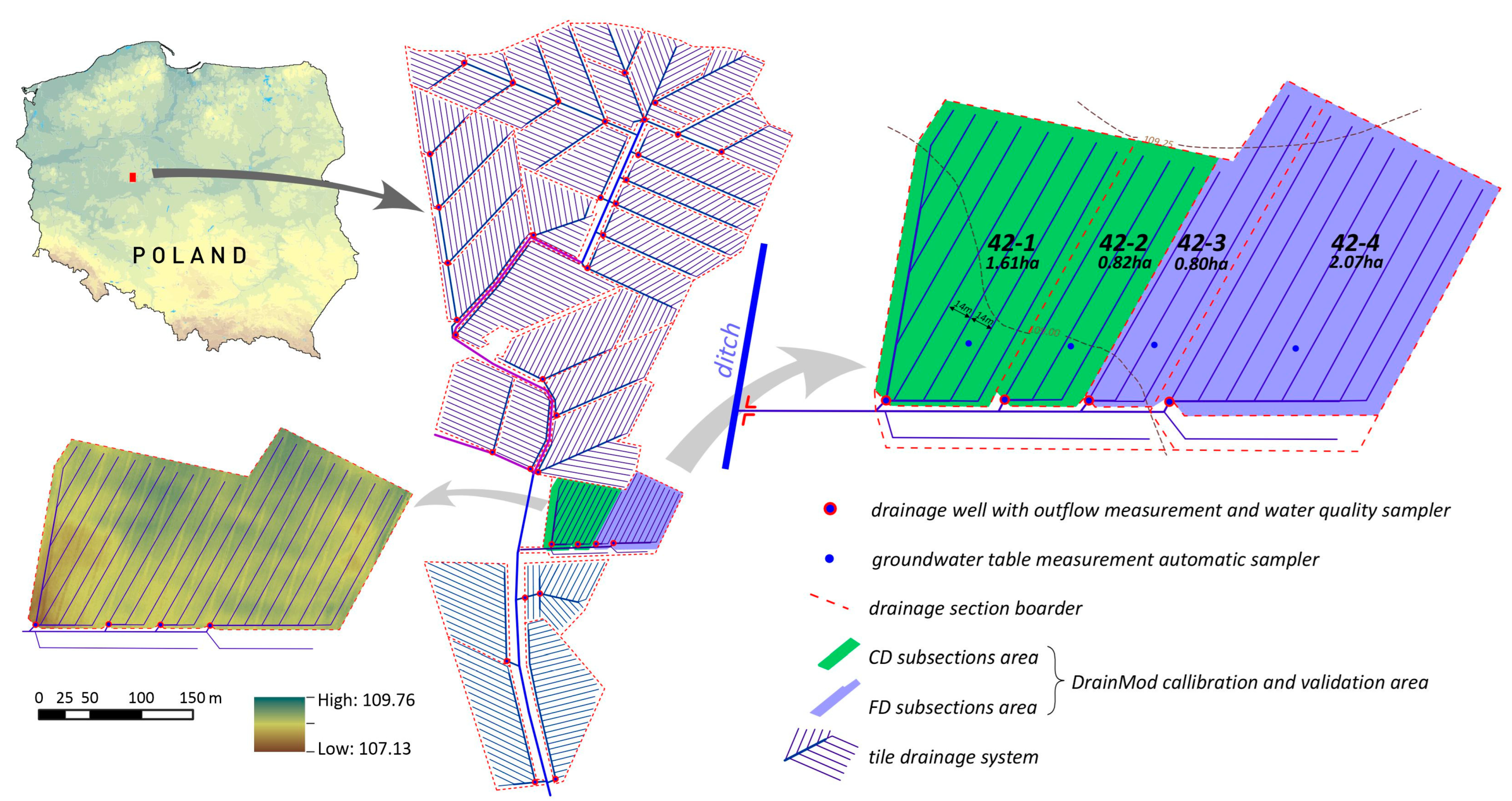
The tile-drained agricultural field Ostrowo Szlacheckie (52°21′38.5″ N, 17°36′34.2″ E, elevation 108.38 m above sea level) is located in the central-western part of the Wielkopolska region (Figure 1). The study site is located near a small village, and the agricultural land is used by a private farm that specializes in crop production and cattle breeding. It is located in the central part of the Wielkopolska Lakeland within the Września Plain. Drainage water is discharged directly into a tributary from Gulczewo, which drains into the Rudnik watercourse. The site is hydrographically located in the Warta Water Region. It is in a moderate climate zone, with an annual average precipitation of 521 mm and annual average temperature of 8.8 °C (1951–2020) according to the Poznan meteorological station.

The subsurface tile drainage network was made of PVC pipes using trenchless technology, and it was installed in the 1980s. The standard life expectancy of a network made of plastic perforated pipe used in subsurface drainage is about 50 years. All divisions of this drainage facility have been drained, without problems, for more than 40 years. As can be seen in Figure 1, some of the drainage divisions are characterized by a fairly large area. Water is discharged into the drainage ditch from 22 drainage divisions. The area of drainage sections ranges from 2.53 to 12.54 ha, while for the drainage network system it is about 107 ha. The study included the drainage section No. 42 of 5.30 ha, where the effect of CD on reducing drainage outflows and reducing NO₃-N losses was analyzed. The area is characterized by flat terrain, with slopes of less than 1%. This type of relief, along with homogeneous soil parent materials, causes the soils of the area to be relatively homogeneous. This makes both the depth and spacing of the drains in the entire drainage section essentially the same, at 14 m and 0.9 to 1.0 m b.s.l., respectively. PVC pipes with a diameter of 0.05 m were used. The lateral tiles are connected to the main drain lines (generally from 75 to 150 mm in diameter) that run along the edge of each field. This main drain is connected to an outlet draining into an adjacent drainage ditch. The soils have been classified as Gleyic Luvisols [59], which developed from glacial till. In the soil profile, the surface and subsurface horizon below the argic horizon have a similar sandy loam texture (

Table 1. Average values of soil properties within drainage section No. 42.

Parameter	Unit	Soil Horizon
		Ap	Bt	Cg or Ck	Ckg
Horizon thickness	cm	36.0	20.75	29.5	60.0
sand content (0.05–2.0 mm)	%	70	64	67	64
silt content (0.002–0.05 mm)	%	21	16	16	19
clay content (<0.002 mm)	%	8	20	18	17
soil bulk density	g cm−3	1.62	1.77	1.74	1.84
organic carbon content Corg	%	1.48	0.61	0.38	0.19
Soil hydraulic parameters
saturated water content	cm3 cm−3	0.358	0.315	0.326	0.298
α	cm−1	0.0412	0.0511	0.0620	0.0443
n	-	1.2967	1.1620	1.1910	1.1522
saturated hydraulic conductivity	cm day−1	43.5	11.8	14.8	7.5
water drainage capacity	cm3 cm−3	0.127	0.076	0.098	0.062
plant available water	cm3 cm−3	0.172	0.127	0.134	0.115

Note(s): α and n—parameters of the Van Genuchten equation.

). The subsurface “argic” horizon has a higher clay content than the overlying horizons and sandy clay loam texture.

Soil parameters were obtained on the basis of detailed field investigations carried out in experimental drainage section 42. In autumn 2018, after harvesting, eight soil pits were made in order to determine the soil morphological properties according to the FAO [59] and soil sampling guidelines. From each distinguished horizon or subhorizon of pedon, eight samples of undisturbed structure (four to assess the soil water retention curve and four to assess the soil bulk density), and three samples with the disturbed structure were collected (from three walls of the soil pit). The soil texture was analyzed by a combination of the hydrometer and wet-sieve methods, [60] and was then classified following the USDA guidelines [61]. Carbonate content (CaCO₃) was determined by applying Scheibler’s volumetric method, and the soil organic carbon content was determined by dry combustion in a Multi N/C 3100 apparatus (Analytik Jena). Soil bulk density (BD) was quantified by the core method in a cylindrical sampler of 100 cm³ [62]. The soil water retention properties were determined using Richards chambers (from 0 to −100 kPa) and the method of using water vapor pressure over a solution of sulfuric acid (from −100 kPa to −1500 kPa) [63,64]. To analyze soil water retention, RETC software was applied to represent the soil water retention curve in the parameters of the van Genuchten equation using the Mualem approach (m = 1 − 1/n) [65,66]. The constant hydraulic water gradient method was used to determine the saturated hydraulic conductivity [67]. The basic properties of the soil are listed in Table 1.

The meteorological data used in the current study were measured at the meteorological station at Sokołowo, 3 km southwest of the Ostrowo Szlacheckie field. As an input date to the DRAINMOD model, a weather file was generated where the measured precipitation (P) and minimal and maximal air temperature (T) were provided at a daily time step from March to September of 2019 and 2020. These data were used to calibrate and validate the model.

GWT was monitored using pressure sensors, called Solinst LTC Leveloggers and Barologger Edge, which were installed in the piezometric wells of section No. 42 to measure GWT on an hourly basis. One well was located on each subsection plot at the midpoint between two drains to increase the accuracy of the monitoring (Figure 1). Measurements were carried out from the beginning of 2019 until the end of August 2021.

Drainage water quality samples were collected manually from February 2019 to June 2020, when the outflow was observed during field work. The samples of 1000 mL polyethylene bottles were collected twice weekly and submitted to the laboratory at the temperature of 4 °C, and were and analyzed in the laboratory within 48 h of their collection. The pH and EC were measured with a pH electrode and conductivity meter, respectively, on unfiltered and unacidified samples. The content of NO₃-N in drainage water was analyzed using the spectrophotometric method in accordance with the standard PN-EN 26777:1999 [68]. Every sample determination was made in duplicate, and the data are presented as averaged values.

2.2. Modeling Procedure

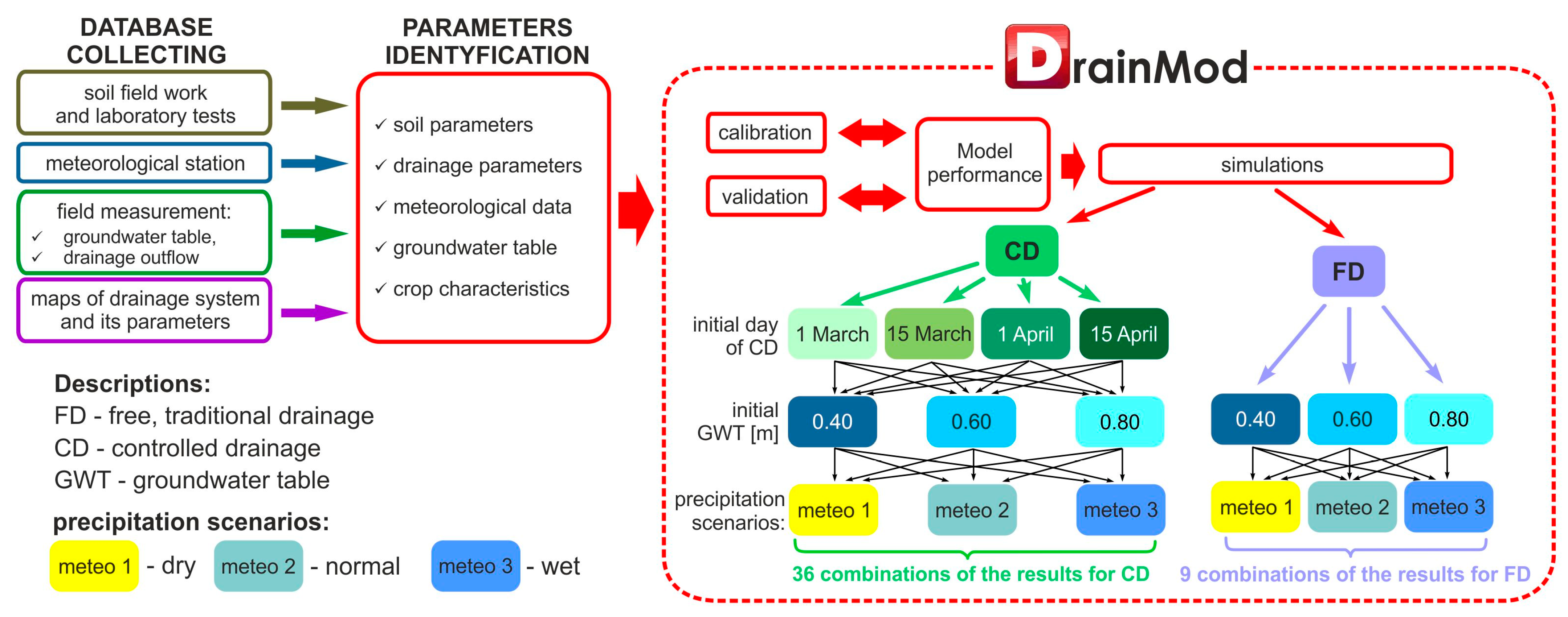
The established research procedure for hydrological modeling of the effect of CD application versus FD on GWT, subsurface outflow, and surface runoff from the drainage facility includes four tasks. The first basic task is the preparation of data from field measurements, laboratory tests, and data analysis of the drainage facility (Figure 2). Based on these, a homogeneous geodatabase of data was created, representing input data consistent with the standard DRAINMOD model. This is a deterministic model that allows one to simulate the hydrology of an artificially subsurface drainage field based on water balance equations. The model can predict drainage outflows, surface runoff, evapotranspiration, lateral seepage, and vertical seepage [44]. The second task involved identifying model parameters, preparing the model, and performing model calibration and validation. The third task was to perform simulations of various scenarios of assumed factors such as the start date of the CD system (none in the case of FD), and initial GWT and meteorological variants, including the amount of precipitation for dry, wet and normal years. The fourth and final task was to subject the obtained results to statistical analysis.

Thirty-six and nine types of scenario analysis were conducted to study the effects of applied CD and FD practices on the drainage outflow at the scale of the drainage facility. The parameters used in the scenario analysis were as follows: different meteorological conditions including precipitation (dry, wet and normal periods), the initial level of GWT on 1 March, the start date of the simulation, three different variants of 0.40, 0.60 and 0.80 m b.s.l., and CD practice start dates of 1 March, 15 March, 1 April, and 15 April (Figure 2). The initial GWT is required by DRAINMOD for running the hydrology simulation. All analyses were performed for a drain spacing of 14 m.

Simulations were performed for different scenarios of meteorological conditions, including precipitation, for the periods from 1 March to 30 September, on the basis of historical data made available on the website by the Institute of Meteorology and Water Management—National Research Institute (IMGW-PIB) (available online: https://danepubliczne.imgw.pl/ (accessed on 30 September 2021)) for the Poznan meteorological station, for the period of 1961–2020. The annual mean of total precipitation was calculated as 527 mm. For each of the wet, dry and normal year scenarios, 10 years were selected from the multi-year data. The meteorological data used in simulations are presented in

Table 2. Basic statistics on annual precipitation, mean annual maximum, and minimum temperature for 10 selected dry, wet, and normal years.

	Dry			Wet			Normal
	P [mm]	Tmax [°C]	Tmin [°C]	P [mm]	Tmax [°C]	Tmin [°C]	P [mm]	Tmax [°C]	Tmin [°C]
Range	275–403	11.96–15.41	2.88–6.45	632–772	11.83–13.84	3.79–6.14	494–551	10.95–14.35	3.36–6.09
Average	355	13.62	4.71	689	12.99	4.80	519	12.73	4.34
SD	37.31	1.09	0.95	50.15	0.61	0.71	18.26	1.11	0.90

.

It was assumed that the initial state of GWT was at 0.80 m b.s.l. on the simulation start day (1 March). Thus, the year preceding the simulation was dry, while in the case of the initial state of 0.40 m b.s.l., the year preceding the simulation was wet.

The drainage coefficient was set at 0.011 cm, which was used for the effective radius of drains. The maximum surface storage was set as 0.005 m, and Kirkham’s depth for flow to drains was assumed to be 0.5 cm. The drainage coefficient setting was 1.4 cm day⁻¹. The depth to the impermeable layer was set at 4.00 m. We initiated the DRAINMOD soil-related parameters based on the soil properties identified in the previously mentioned field and laboratory studies. In addition, the soil tool package included in DRAINMOD was used to estimate the parameters of the Green-Ampt infiltration model, the drainage volume–water table depth relationship, and the upflux–water table depth relationships.

2.3. Calibration and Validation of the Model

DRAINMOD was calibrated and validated according to the procedure described by Skaggs et al. [69] by comparing the modeled GWT to field measurements. The data collected during 2019 were used for model calibration, while data measured in 2020 were used for model validation. The overall goal of the model calibration was to optimize the model input parameters within reasonable ranges to minimize the difference between the measured and modeled GWT. During the calibration process, the saturated hydraulic conductivity of layer/horizon, the thickness of the restrictive layer, and the hydraulic head at the bottom of the restrictive layer focus were adjusted. The performance of the model was assessed using the following statistical indicators during the calibration and validation procedure: root mean square error (RMSE), the coefficient of residual mass (CRM), the index of agreement (d), and the model efficiency index (EF) [70,71]:

$$RMSE={\left({\sum }_{i=1}^n(P_i-O_i{)}^2/n\right)}^{1/2}$$

(1)

$$CRM=\frac{\left({\sum }_{i=1}^n{P}_i-{\sum }_{i=1}^n{O}_i\right)}{{\sum }_{i=1}^n{O}_i}$$

(2)

$$d=1-\frac{{\sum }_{i=1}^n(P_i-O_i{)}^2}{{\sum }_{i=1}^n(\left|O_i-O\right|+\left|P_i-O\right|{)}^2}$$

(3)

$$EF=1-\frac{{\sum }_{i=1}^n(O_i-O{)}^2-{\sum }_{i=1}^n(P_i-O_i{)}^2}{{\sum }_{i=1}^n(O_i-O{)}^2}$$

(4)

where n is the total number of observations, O_i is the observed value of the ith observation, P_i the predicted value of the ith observation, and O the mean of the observed values (i = 1 to n). The identification of the model parameters and the procedure for its calibration and validation were carried out as described in detail by Sojka et al. [72].

2.4. Calculations of Drainage Water Quality

Based on the sampled drainage outflows, analyses were performed to determine the characteristic concentrations of nutrient compounds (

Table 3. The concentration of nutrients from drainage outflows of the analyzed drainage division during the 2019 study period.

Nutrient	Concentration [mg/L]
	Range	Average	SD	V
NO3-N	14.01–87.98	42.33	17.33	300.35
NO3	62.03–389.50	187.37	76.72	5886.36

) from drainage subdivision 42. Nitrogen compound loads leached from the catchment were then calculated. These loads were calculated on the basis of the modeled outflows from the catchment using FD and CD practices under different control initiation scenarios in dry, wet and normal years, and with average concentrations of nutrient compounds. Based on the calculated nitrogen unit loads, the amount of nutrient leaching from the entire drainage facility was estimated.

Drainage outflows indicated that the highest proportion of NO₃-N in total nitrogen reached 94%, and that it is the main form of nitrogen. In the case of the values of this nitrogen, speciation ranged from 14.01 to 87.98 mg/L. The content of total nitrogen ranged from 17.48 to 92.02 mg/L.

2.5. Measures of Accuracy and Variable Correlation

Basic statistical parameters were calculated for each drainage and initial GWT variants for dry, wet and normal years. A one-dimensional analysis of variance (ANOVA) and a Tukey’s HSD test were used to confirm the existence of uniform (α = 0.05) groups of combinations (applications of FD and CD practices on a drainage site) in terms of varying meteorological conditions for dry, wet and normal years. Calculations were performed using the Statistica 13.3 program (TIBCO Software Inc., Palo Alto, CA, USA).

3. Results

3.1. Quality of the Model

The results of the calibration and validation are shown in

Table 4. Results of calibration and validation of the DRAINMOD model for GWT prediction.

Year	RMSE [m]	CRM [%]	d [−]	EF [−]
calibration
2019	0.054	2.1	0.960	0.961
validation
2020	0.069	2.9	0.947	0.947

. The RMSE values were 0.054 m and 0.069 m, while the CRM was 2.1% and 2.9% for calibration and validation, respectively. The d and EF values for calibration were 0.960 and 0.961, respectively, while for validation the value was 0.947. The results of the calibration and validation are shown in Table 4. The obtained values of RMSE, CRM, d and EF for both calibration and validation indicate a very high agreement between the measured and modeled GWT. This indicates that the DRAINMOD model has been well configured, and can be used to simulate the effects of different CD scenarios on the dynamics of the GWT and the drainage outflow of the drained soils.

3.2. Groundwater Table Depth

The initial GWT had no significant effect on the variation of the average depth of the GWT for FD practice. The application of the CD practice from 1 March for the distinct groups of dry, wet and normal years results in the highest mean values of GWT in the analyzed period. For this CD practice, three different groups: a, b and c, were distinguished in each year (dry, normal and wet) (

Table 5. Average GWT for dry, wet and normal years for drainage variants of the FD and CD of different initial GWT variants.

Drainage Variants		Initial GWT Variants (cm b.s.l.)	Average GWT for Years (cm b.s.l.)
			Dry		Wet		Normal
FD		40	155.7 ± 0.91	e,f	150.8 ± 0.89	g,h	152.3 ± 0.90	f,g
		60	156.4 ± 0.89	e,f	151.3 ± 0.88	g,h	152.8 ± 0.88	f,g
		80	157.6 ± 0.87	f	152.1 ± 0.86	h	153.6 ± 0.87	g
CD	1.03	40	126.2 ± 1.09	a	117.0 ± 1.07	a	119.3 ± 1.09	a
		60	136.5 ± 1.01	b	127.1 ± 0.98	b	129.7 ± 1.00	b
		80	148.0 ± 0.94	c	138.8 ± 0.90	c	141.6 ± 0.92	c
	15.03	40	151.0 ± 0.94	c,d	142.7 ± 0.88	c,d	146.5 ± 0.91	c,d
		60	152.1 ± 0.92	c,d,e	143.6 ± 0.87	d,e	147.4 ± 0.89	d,e
		80	153.7 ± 0.90	d,e,f	145.2 ± 0.85	d,e,f	148.7 ± 0.88	d,e,f
	1.04	40	155.0 ± 0.90	d,e,f	147.1 ± 0.87	e,f,g	150.1 ± 0.89	d,e,f,g
		60	155.7 ± 0.89	e,f	147.6 ± 0.86	e,f,g	150.6 ± 0.88	d,e,f,g
		80	157.0 ± 0.87	f	148.6 ± 0.84	f,g,h	151.4 ± 0.86	e,f,g
	15.04	40	155.4 ± 0.90	d,e,f	149.0 ± 0.87	f,g,h	150.8 ± 0.89	d,e,f,g
		60	156.1 ± 0.89	e,f	149.5 ± 0.85	g,h	151.3 ± 0.88	e,f,g
		80	157.4 ± 0.87	f	150.4 ± 0.83	g,h	152.0 ± 0.86	f,g

Note(s): Different letters indicate significant differences (p ≤ 0.05) between variants for each group of years according to a Tukey’s test.

), indicating significant differences in average GWT between the three variants of the initial GWT. The shallowest water table occurred at an average depth of 117 cm b.s.l. in wet years for the shallowest initial GWT (40 cm). Under normal and wet conditions, the practice variant CD—15 March with 40 cm, 60 cm and 80 cm initial GWT, caused a significant increase in the average GWT compared to FD. The other CD variants (1 April, 15 April) have practically no significant effect on the average GWT values, which are the same as they are for FD. For dry years, this drainage variant CD—15 March, in relation to FD, is effective only for the initial GWT at 40 cm.

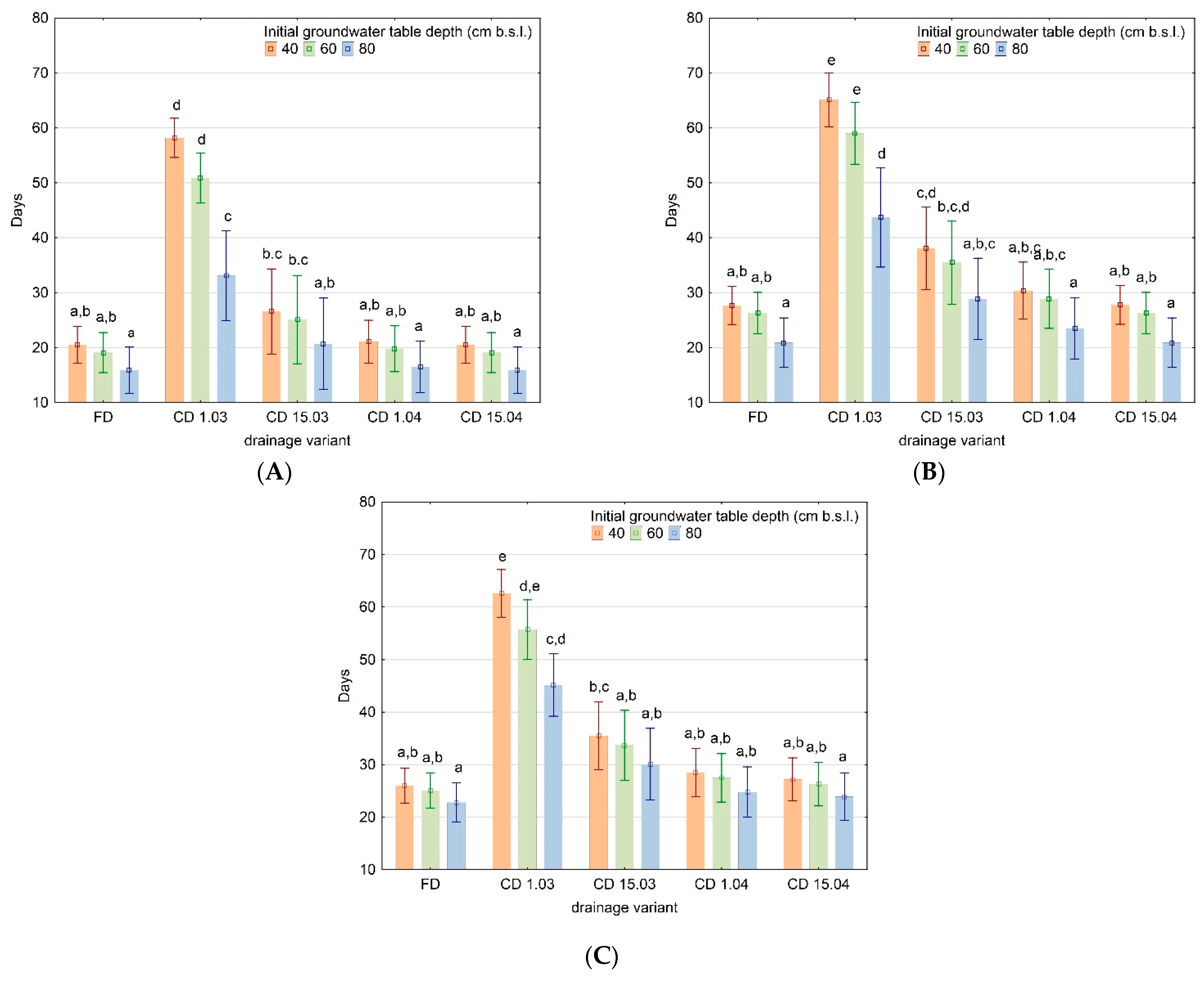
If the CD practice is used for different start options, this allows for a longer period during which the water table is above the drainage network (Figure 3). The most effective variants of this method involve starting to control the outflow on 1 March for different variants of the initial depth of GWT for the three groups of dry, wet and normal years. This increases the number of days that the GWT stays above the level of the drainage network. In this case, in applying CD to a drainage network, it was determined that the residence time of GWT over drains for dry, wet and normal years were 47, 56 and 55 days on average, respectively. For CD variants beginning on 15 March, a slightly lower number of days were obtained in all three year scenarios. The average number of days was 24, 34, and 33 for dry, wet and normal years, respectively. For the scenarios in which the CD was started on 1 April and 15 April, the values obtained indicated that this CD procedure was even less important, and was similar to the FD practice.

3.3. Subsurface Drainage Outflows

Using the 1 March CD for all three precipitation scenarios, the simulation results indicate three homogeneous groups a, with the smallest value of average outflow (

Table 6. Average subsurface drainage outflows for the dry, wet and normal for drainage variants of FD and CD of different initial GWT variants.

Drainage Variants		Initial GWT (cm b.s.l.)	Average Subsurface Drainage Outflows (mm)
			Dry		Wet		Normal
FD		40	48.0 ± 17.0	f	52.4 ± 13.7	i	52.2 ± 11.8	g
		60	31.8 ± 16.6	d,e	35.8 ± 13.5	f,g	35.7 ± 11.6	e
		80	15.0 ± 15.8	b,c	18.4 ± 12.9	c,d	18.1 ± 11.3	c
CD	1.03	40	0.9 ± 0.2	a	1.1 ± 0.3	a	1.0 ± 0.2	a
		60	0.7 ± 0.3	a	0.7 ± 0.2	a	0.7 ± 0.3	a
		80	0.4 ± 0.3	a	0.4 ± 0.2	a	0.4 ± 0.2	a
	15.03	40	40.7 ± 5.7	e,f	41.9 ± 6.9	g,h	43.6 ± 3.0	f
		60	25.0 ± 5.5	c,d	26.2 ± 6.8	d,e	27.7 ± 3.0	d
		80	8.9 ± 4.9	a,b	10.0 ± 6.1	b,c	11.1 ± 2.8	b
	1.04	40	47.2 ± 16.1	f	49.1 ± 12.3	h,i	49.3 ± 8.3	f,g
		60	31.1 ± 15.7	d,e	32.6 ± 12	e,f	32.9 ± 8.1	d,e
		80	14.5 ± 14.9	b,c	15.4 ± 11.3	c	15.4 ± 7.8	b,c
	15.04	40	48.0 ± 17.0	f	52.3 ± 13.7	i	50.3 ± 8.8	g
		60	31.8 ± 16.6	d,e	35.8 ± 13.4	f,g	33.8 ± 8.7	d,e
		80	15.0 ± 15.8	b,c	18.3 ± 12.8	c,d	16.2 ± 8.3	b,c

Note(s): Different letters indicate significant differences (p ≤ 0.05) between variants for each group of years according to a Tukey’s test.

). For all combinations of CD starting after 1 April and 15 April, the resulting average subsurface drainage outflows are similar to those of FD. Furthermore, no significant differences were found between the combinations for wet and normal years.

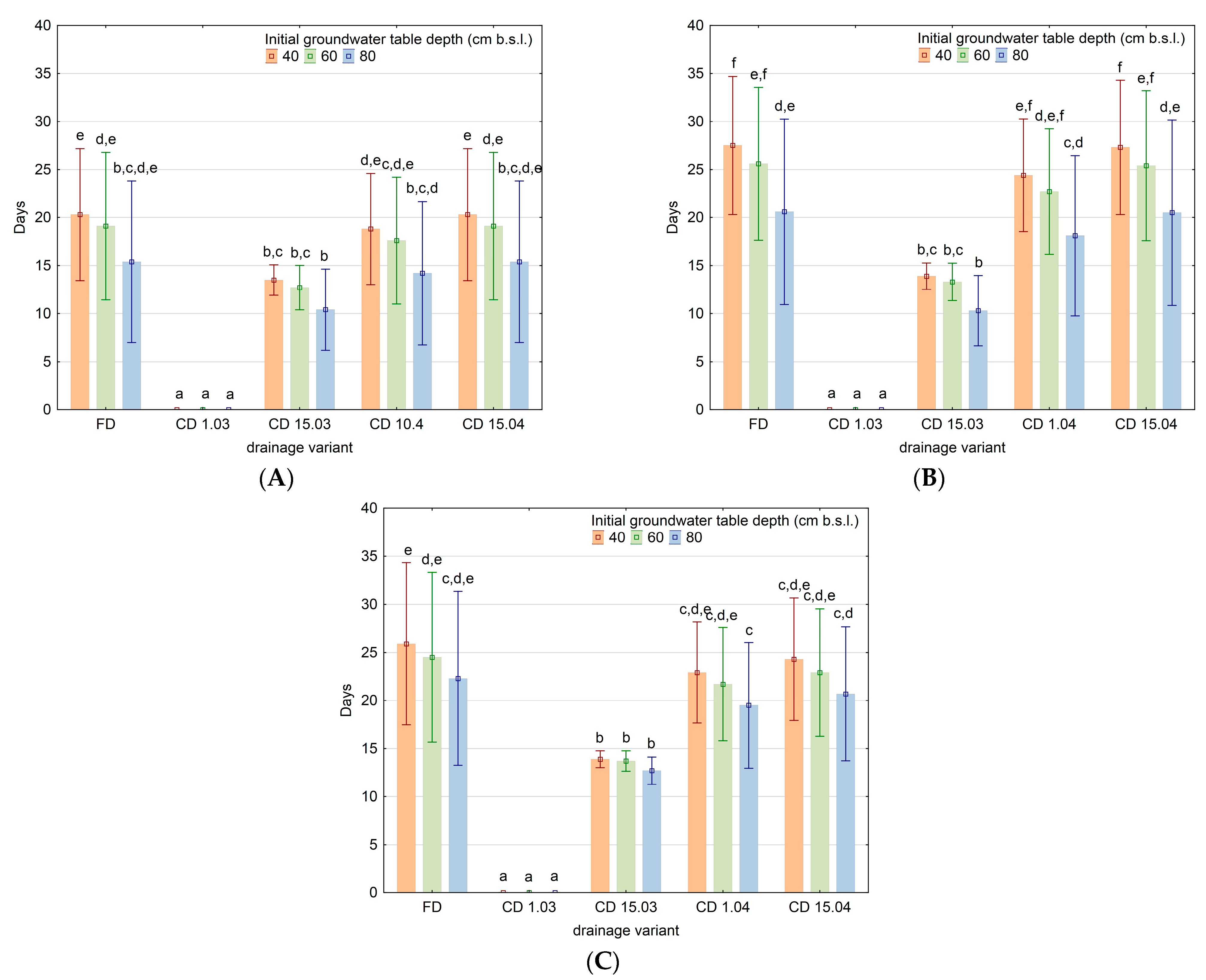
The use of CD makes it possible to reduce the number of days with drainage outflow in comparison to FD (Figure 4), thereby extending the period during which GWT is retained on the site. The most effective option is to start retaining outflow on 1 March for all variants. In each group of years, a homogeneous group a is indicated for each variant, indicating the absence of days with recorded drainage outflow on that date. When starting the withholding of the drainage outflow on 15 March for the dry and wet years of the initial GWT variants, similar results were obtained. When the CD practice started on 1 April and 15 April, there was a similar increase in the number of days for each GWT variant. In addition, identical homogeneous groups were observed for the indicated initial GWT variants in these years.

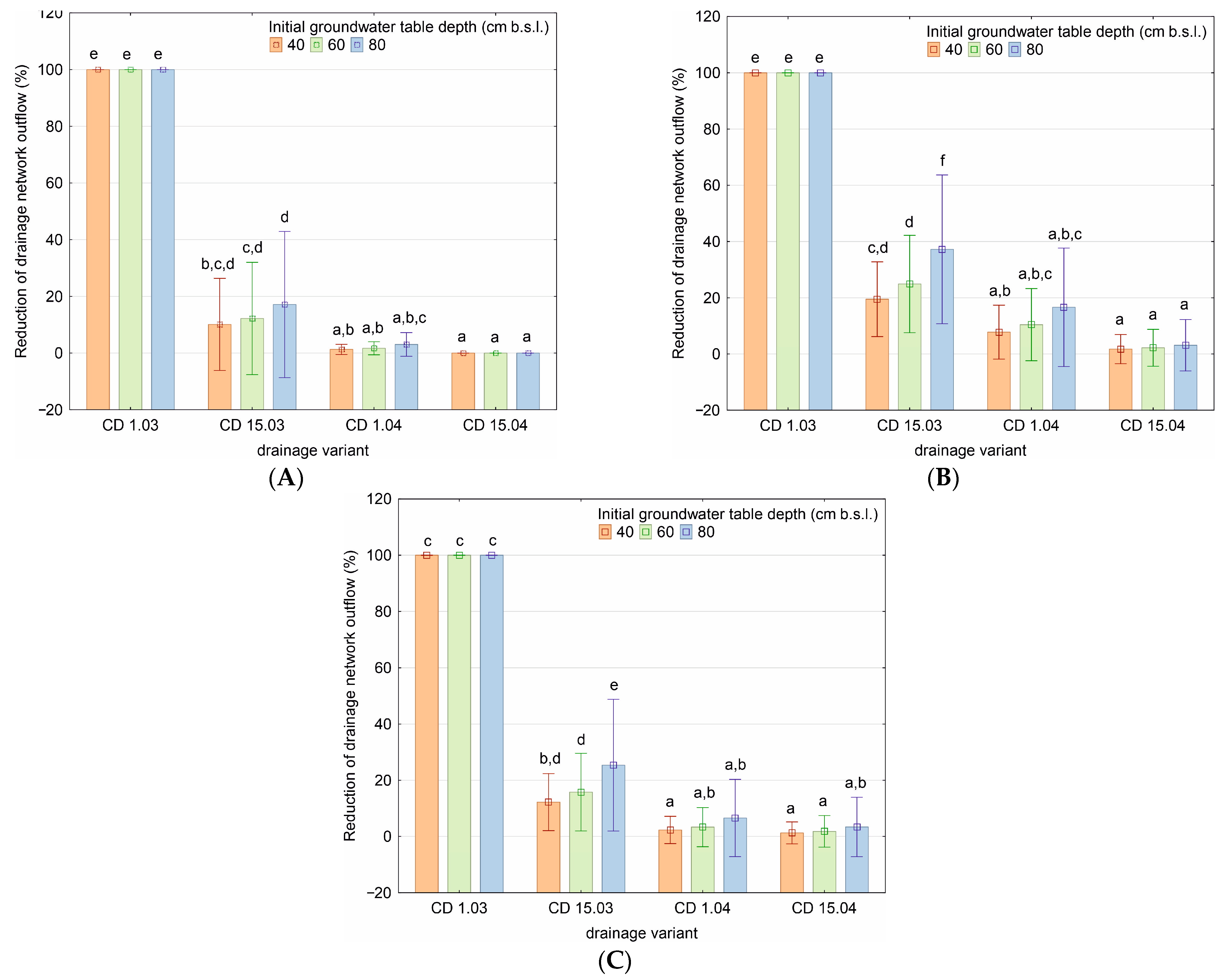
For the adopted precipitation scenarios, the greatest effects of reducing drainage outflows by CD were obtained in the cases where the outflow blockage began on 1 March (Figure 5). Accordingly, for the cases starting from the setting of all the initial GWT variants, outflows can be reduced by up to 100%. If the date for blocking outflows is moved to 15 March, the reduction is significantly lower, with an average of 13%, 27% and 19%, for dry, wet and normal years, respectively. The start of CD practice on 1 April showed outflow reductions of 1.3–3.0%, 7.8–16.6%, and 2.3–6.5% for dry, wet and normal years, respectively. No effect was observed when the blockage of outflows started on 15 April.

3.4. Surface Runoff

Surface runoff is particularly important in terms of erosion and the loss of nitrogen compounds. The simulation results show that surface runoff is small (Figure 6). The calculations showed that for the flat terrain analyzed, CD practices do not have a statistically significant effect on differences in surface runoff in either dry, wet, or normal years. Slight differences, although not statistically significant, may relate to the practice of early CD on 1 March in the case of a shallow GWT (40 and 60 cm b.s.l.). This means that under these conditions, the runoff process may lead to higher losses of nitrogen compared to other CD variants.

3.5. Nitrate Outflow Reduction

The analysis of NO₃-N loads indicated a significant reduction in discharge with drainage outflow from the analyzed subdivisions when CD was applied on 1 March in all precipitation scenarios (

Table 7. Average NO₃-N (kg ha⁻¹) loads for drainage subdivisions 42-2 and 42-3 for dry, wet, and normal years.

Drainage Variants		Initial GWT (cm b.s.l.)	Load NO3-N (kg ha−1)
			Dry		Wet		Normal
FD		40	20.32	f	22.16	i	22.11	g
		60	13.46	d,e	15.16	f,g	15.11	e
		80	6.37	b,c	7.79	c,d	7.67	c
CD	1.03	40	0.00	a	0.00	a	0.00	a
		60	0.00	a	0.00	a	0.00	a
		80	0.00	a	0.00	a	0.00	a
	15.03	40	17.25	e,f	17.75	g,h	18.46	f
		60	10.60	c,d	11.08	d,e	11.75	d
		80	3.79	a,b	4.23	b,c	4.68	b
	1.04	40	20.00	f	20.77	h,i	20.88	f,g
		60	13.16	d,e	13.80	e,f	13.90	d,e
		80	6.12	b,c	6.52	c	6.51	b,c
	15.04	40	20.32	f	22.14	i	21.28	g
		60	13.46	d,e	15.13	f,g	14.29	d,e
		80	6.37	b,c	7.76	c,d	6.86	b,c

Note(s): Different letters indicate significant differences (p ≤ 0.05) between variants for each group of years according to a Tukey’s test.

). This is indicated by the classification of this date into a homogeneous group a with a range of 0.15 to 0.45 kg ha⁻¹. The CD practice, which began on 1 March, allows for a reduction in load leaching from 6.22 to 21.71 kg ha⁻¹ compared to FD. Starting the CD on 15 March in the variant of the initial GWT at 80 cm indicates lowering the NO₃-N load of 2.58–3.56 kg ha⁻¹. The other two dates for the start of the CD indicate similar results to the FD practice. If the initial depth of withholding the outflow is considered, the largest average values of loads are for 40 cm b.s.l., while the smallest are for 80 cm b.s.l. Similar differences in NO₃-N load between wet and dry years were obtained for FD and CD variants that started on 1 April at 1.39–1.84 kg ha⁻¹.

As expected, a 100% reduction in NO₃-N loads for CD practice started on 1 March (

Table 8. NO₃-N reduction of drainage network for different drainage variants in dry, wet, and normal years.

Drainage Variants		Initial GWT (cm b.s.l.)	Reduction of NO3-N (%)
			Dry		Wet		Normal
CD	1.03	40	100	e	100	e	100	c
		60	100	e	100	e	100	c
		80	100	e	100	e	100	c
	15.03	40	10.11	b,c,d,	19.48	c,d	12.20	b,d
		60	12.20	c,d	24.90	d	15.77	d
		80	17.13	d	37.21	f	25.37	e
	1.04	40	1.30	a,b	7.77	a,b	2.29	a
		60	1.70	a,b	10.44	a,b,c	3.31	a,b
		80	3.04	a,b,c	16.63	a,b,c	6.54	a,b
	15.04	40	0.00	a	1.74	a	1.24	a
		60	0.00	a	2.22	a	1.78	a
		80	0.00	a	3.13	a	3.35	a,b

Note(s): Different letters indicate significant differences (p ≤ 0.05) between variants for each group of years according to a Tukey’s test.

). For the two-week later start of CD practice, the reduction was significantly smaller. This is considerably higher than the later dates when CD was started. For dry years, there was no reduction in load leaching for the 1 April CD.

The total annual NO₃-N loads discharged from the whole drainage system are a fairly accurate representation of the loads reported for discharge from the drainage network. The lowest loads were observed for the CD practice that started on 1 March for each precipitation scenario (

Table 9. Total NO₃-N removed from the surface of the entire drainage facility for different drainage variants in dry, wet, and normal years.

Drainage Variants		Initial GWT (cm b.s.l.)	NO3-N (kg)
			Dry	Wet	Normal
FD		40	2166.87	2363.40	2357.79
		60	1435.21	1616.44	1611.56
		80	679.19	830.53	818.15
CD	1.03	40	42.60	48.20	45.01
		60	30.07	31.57	32.02
		80	16.24	17.99	18.32
	15.03	40	1839.40	1893.56	1969.08
		60	1130.39	1181.28	1252.61
		80	403.77	450.69	499.15
	1.04	40	2132.58	2214.98	2226.90
		60	1403.88	1471.62	1482.89
		80	652.60	695.27	694.30
	15.04	40	2166.87	2360.73	2269.10
		60	1435.21	1613.80	1523.53
		80	679.19	828.02	731.78

). The later dates for the start of CD give similar results for the removal of loads from the drainage system to the FD practice. The highest values were observed for the FD practice for wet years in all GWT variants.

4. Discussion

The results obtained in this study indicate that it is possible to effectively increase the groundwater table, reduce subsurface outflow from the drainage network, and reduce NO₃-N losses through CD practices. Thus, CD solutions provide opportunities to insert more water and NO₃-N into the soil-water-atmosphere-plant system. For an area with slopes not exceeding 1% where the soils have been developed from sandy loam, significant CD efficiency occurs when outflows are blocked during 1–15 March. Blocking drainage outflows at a later date does not lead to a significant increase in GWT or a reduction in water and nitrate losses compared to FD.

Reducing water outflows with CD practice starting at 1–15 March reduces outflows by 37–100%, 25–100%, and 17–100%, in wet, normal and dry years, respectively. The ranges of reduction in drainage outflows obtained in this study for the recommended time of CD implementation (1–15 March) correspond to those reported by other authors [44,73,74,75,76,77,78,79,80]. Skaggs et al. [73,75,76] achieved an average reduction in outflow of 6–42% with annual precipitation ranging from 907 to 1760 mm. Similar values were reported by Williams et al. [78], Negm et al. [79], and Youssef et al. [80]. In contrast, El-Sadek et al. [81] obtained the smallest reduction in outflow (0.8–4.1%) in sandy soil, with an average annual rainfall of 868 mm. Variations in the results of the effect of CD on drainage outflow reduction may be attributable to different climatic conditions, soil properties, and technical parameters of the drainage network [78]. Our results showed that for years differing in terms of annual precipitation, the reduction in drainage outflow varies even when starting the CD practice on the same dates and with the same initial GWT. The maximum amount of water that can be saved by the CD practice starting on 1 March with an initial GWT of 40 cm is 48–52 mm. Ale et al. [76] obtained an average annual reduction in drainage outflow of 51 mm for the Hoagland Ditch watershed. The later decision (1–15 April) to use CD under the analyzed conditions does not reduce the duration (days) of drainage outflows compared to FD.

In addition to regulating drainage outflows through CD practices, it is also important to control GWT, especially from the point of view of the water needs of plants. Furthermore, changes in GWT are a valid parameter in assessing the effectiveness of CD. The obtained results showed the highest average GWT for the CD practice starting on 1 March for all water depth variants (40 cm, 60 cm and 80 cm). The 1 March start date of CD practice results in an increase in the average GWT for the March to September period. The highest values of GWT increase were observed for the 40 cm initial variant. A similar maximum rise of the GWT (36 cm) during the growing season was observed by Ale et al. [74]. As drainage outflows become blocked, the time of the GWT above the drains increases. However, for variants with an initial GWT in the 40–80 cm range, the number of days of this extension in relation to FD is similar for both dry (17–37 days) and wet (23–37 days) years. In relation to FD, the application of CD on 15 March also results in a significant increase in average GWT, and thus an increase in the number of days with the GWT above the drains. However, these effects are significantly smaller than for those resulting from the blocking of the drainage outflow on 1 March.

Along with the blockage of drainage outflows and rising GWT, the potential danger of generating surface runoff increases [82,83]. In analyzed flat terrain, the results of the statistical analyses showed that CD practices have no significant effect on the increase in surface runoff. Slightly higher values of surface runoff, although not statistically significant, may relate to the CD practice starting on 1 March when the initial GWT is shallow (40 and 60 cm).

CD practices can have a significant impact on the reduction of nutrient losses. This mainly concerns NO₃-N, which can be easily leached from the soil to the drainage water. The results indicated that CD practice application use on 1 March can even reduce NO₃-N losses completely (100%). The losses at later dates were similar to those obtained in FD practice. Liu et al. [84] reported that the total reduction in NO₃ losses (91% and 99%) with CD were closely related to reduced drain outflow rates (88% and 98%). Tolonio and Borin [85,86] found that CD reduced the outflow by 69% and 81% compared to FD, respectively. They also reported that CD reduced annual nitrogen losses by 92% (from 29 to 2 kg NO₃-N ha⁻¹) compared to FD, where losses were 46 kg NO₃-N ha⁻¹. Wang et al. [87] concluded that the implementation of CD reduced the loss of NO₃-N by 20.53% and reduced the amount of drained water by 19.23%. Some studies have demonstrated that CD has been effective in reducing nitrate-nitrogen loss due to a reduction in drainage outflow [88]. In the case of 15 March, the NO₃-N loss reduction was about 10–17%, 12–25%, and 19–37% for dry, normal, and wet years, respectively. A similar reduction of 27–32% was reported by Ma et al. [89]. Salazar et al. [90] observed higher NO₃-N losses for an annual rainfall of 722 mm (7.9–10.1 kg ha⁻¹) than for an annual rainfall of 578 mm (0.1–0.4 kg ha⁻¹) from a plot with CD practice. Poole et al. [91] found that CD reduced NO₃-N export by 30%, with an average annual reduction of 6.3 kg ha⁻¹ per year⁻¹. According to our results, the entire drainage facilities of the investigated area of CD can reduce the total amount of NO₃-N from 830–2363 kg to 18–48 kg compared to FD in wet years. This confirms the most significant benefit of CD, as the reduction in drainage outflows reduces the NO₃-N load. This will significantly reduce the supply of nitrates of agricultural origin to water bodies, thereby improving the ecological status of surface waters by significantly reducing the degree of eutrophication [15,16].

The relevance of the research is important in relation to the current, ageing infrastructure and the potential design of new subsurface drainage infrastructure for agricultural fields in Poland. Climate change is influencing adaptation measures in agriculture in terms of water management. Adaptive drainage water management strategies, e.g., CD, for drained agricultural landscapes are increasingly being implemented to identify opportunities for water storage or diversion. Answers are being sought as to how drainage systems should be designed and used in the future. This is influenced by the changing approach to drainage, from an emphasis on rapid one-way removal of all water, to investigating how water can be controlled within agricultural fields for production and water quality purposes.

5. Conclusions

The above presented results and their analyses allow us to draw the following conclusions:

• The control of water outflow from the drained field in the Wielkopolska region using CD practice proved to be the best strategy when starting from 1 to 15 March. The simulation showed the best performance by reducing the drainage outflow and thus reducing nutrient losses. An increase in the groundwater table during CD practice does not affect the surface runoff in relation to FD.
• Starting the CD practice on 1 to 15 March can reduce drainage outflow by 37–100%, 25–100%, and 17–100% in wet, normal, and dry years, respectively. The amount of drainage outflow that will result from the later decision (1 to 15 April) to run the CD is statistically similar to those drainage outflows for the FD.
• In dry years, starting CD practices in the period of 1 to 15 March makes it possible to significantly raise the groundwater table and to extend its duration above the level of drains, by an average of 33–58 days when compared to FD. In wet and normal years, the extension is similar, at about 55 days. An increase of groundwater in the analyzed flat arable area does not affect the surface runoff.
• The most effective reduction of NO₃-N losses was observed for CD practice from 1 to 15 March. This reduction is approximately twice as high in wet years in comparison to dry years. The later start of CD practices has no significant effect on NO₃-N reduction compared to FD.
• The application of CD under the conditions of the analyzed drainage facility makes it possible to significantly reduce the discharge of NO₃-N. With this technique, it is possible to retain up to 22 kg of NO₃-N per hectare.

References

- Granstedt, A.; Schneider, T.; Seuri, P.; Thomsson, O. Ecological Recycling Agriculture to Reduce Nutrient Pollution to the Baltic Sea. Biol. Agric. Hortic. 2008, 26, 279–307. [Google Scholar] [CrossRef]
- McIsaac, G. Surface water pollution by nitrogen fertilizers. Encycl. Water Sci. 2003, 2003, 950–955. [Google Scholar] [CrossRef]
- Norse, D. Non-point pollution from crop production: Global, regional and national issues. Pedosphere 2005, 15, 499–508. [Google Scholar]
- Smith, L.E.; Siciliano, G. A comprehensive review of constraints to improved management of fertilizers in China and mitigation of diffuse water pollution from agriculture. Agric. Ecosyst. Environ. 2015, 209, 15–25. [Google Scholar] [CrossRef]
- Verhoeven, J.T.; Arheimer, B.; Yin, C.; Hefting, M.M. Regional and global concerns over wetlands and water quality. Trends Ecol. Evol. 2006, 21, 96–103. [Google Scholar] [CrossRef]
- Savci, S. Investigation of effect of chemical fertilizers on environment. Apcbee Procedia 2012, 1, 287–292. [Google Scholar] [CrossRef]
- Rose, L.A.; Sebestyen, S.D.; Elliott, E.M.; Koba, K. Drivers of atmospheric nitrate processing and export in forested catchments. Water Resour. Res. 2015, 51, 1333–1352. [Google Scholar] [CrossRef]
- Nikolenko, O.; Jurado, A.; Borges, A.V.; Knӧller, K.; Brouyѐre, S. Isotopic composition of nitrogen species in groundwater under agricultural areas: A review. Sci. Total Environ. 2018, 621, 1415–1432. [Google Scholar] [CrossRef] [PubMed]
- Lintern, A.; McPhillips, L.; Winfrey, B.; Duncan, J.; Grady, C. Best Management Practices for Diffuse Nutrient Pollution: Wicked Problems across Urban and Agricultural Watersheds. Environ. Sci. Technol. 2020, 54, 9159–9174. [Google Scholar] [CrossRef]
- Lee, C.M.; Hamm, S.Y.; Cheong, J.Y.; Kim, K.; Yoon, H.; Kim, M.; Kim, J. Contribution of nitrate-nitrogen concentration in groundwater to stream water in an agricultural head watershed. Environ. Res. 2020, 184, 109313. [Google Scholar] [CrossRef]
- L 327/1; Directive 2000/60/EC of the European Parliament and of the Council of 23rd October 2000 Establishing a Framework for Community Action in the Field of Water Policy. European Commission: Brussels, Belgium, 2000.
- OJ L 375; Council Directive 91/676/EEC of 12 December 1991 Concerning the Protection of Waters against Pollution Caused by Nitrates from Agricultural Sources. European Commission: Brussels, Belgium, 1991; pp. 1–8.
- OJ L 309; Directive 2009/128/EC of the European Parliament and of the Council of 21 October 2009 Establishing a Framework for Community Action to Achieve the Sustainable Use of Pesticides. European Commission: Brussels, Belgium, 2009; pp. 71–86.
- Kundzewicz, Z.W. Adaptation to floods and droughts in the Baltic Sea basin under climate change. Boreal Environ. Res. 2009, 14, 193–203. Available online: http://www.borenv.net/BER/archive/ber141.htm (accessed on 8 April 2022).
- Poikane, S.; Kelly, M.G.; Herrero, F.S.; Pitt, J.A.; Jarvie, H.P.; Claussen, U.; Leujak, W.; Solheim, A.L.; Teixeira, H.; Phillips, G. Nutrient criteria for surface waters under the European Water Framework Directive: Current state-of-the-art, challenges and future outlook. Sci. Total Environ. 2019, 695, 133888. [Google Scholar] [CrossRef] [PubMed]
- Poikane, S.; Phillips, G.; Birk, S.; Free, G.; Kelly, M.G.; Willby, N.J. Deriving nutrient criteria to support ‘good’ ecological status in European lakes: An empirically based approach to linking ecology and management. Sci. Total Environ. 2019, 650, 2074–2084. [Google Scholar] [CrossRef] [PubMed]
- EEA [European Environment Agency]. European Waters—Assessment of Status and Pressures 2018; EEA Report 7/2018; Publications Office of the European Union: Luxembourg, 2018. [Google Scholar]
- Spinoni, J.; Naumann, G.; Vogt, J.; Barbosa, P. Meteorological Droughts in Europe: Events and Impacts—Past Trends and Future Projections. 2016. Available online: http://www.droughtmanagement.info/literature/EC-JRC_Report%20on%20Droughts%20in%20Europe_2016.pdf (accessed on 8 April 2022).
- Spinoni, J.; Vogt, J.V.; Naumann, G.; Barbosa, P.; Dosio, A. Will drought events become more frequent and severe in Europe? Int. J. Climatol. 2018, 38, 1718–1736. [Google Scholar] [CrossRef]
- Rakovec, O.; Samaniego, L.; Hari, V.; Markonis, Y.; Moravec, V.; Thober, S.; Hanel, M.; Kumar, R. The 2018–2020 Multi-Year Drought Sets a New Benchmark in Europe. Earth’s Future 2022, 10, e2021EF002394. [Google Scholar] [CrossRef]
- Łabędzki, L. Problematyka susz w Polsce. Woda-Sr.-Obsz. Wiej. 2004, 4, 47–66. (In Polish) [Google Scholar]
- Zamorowska, K. Plan Przeciwdziałania Skutkom Suszy—Po raz Pierwszy, za 6 lat Aktualizacja. Available online: https://www.teraz-srodowisko.pl/aktualnosci/rozporzadzenie-przyjecie-plan-przeciwdzialania-skutkom-suszy-MI-9827.html (accessed on 20 April 2022).
- Wanders, N.; Wada, Y. Human and climate impacts on the 21st century hydrological drought. J. Hydrol. 2015, 526, 208–220. [Google Scholar] [CrossRef]
- Kopittke, P.M.; Menzies, N.W.; Wang, P.; McKenna, B.A.; Lombi, E. Soil and the intensification of agriculture for global food security. Environ. Int. 2019, 132, 105078. [Google Scholar] [CrossRef]
- Wreford, A.; Topp, C.F. Impacts of climate change on livestock and possible adaptations: A case study of the United Kingdom. Agric. Syst. 2020, 178, 102737. [Google Scholar] [CrossRef]
- Al-Mukhtar, M. Modeling of pan evaporation based on the development of machine learning methods. Theor. Appl. Climatol. 2021, 146, 961–979. [Google Scholar] [CrossRef]
- Al-Mukhtar, M.; Dunger, V.; Merkel, B. Runoff and sediment yield modeling by means of WEPP in the Bautzen dam catchment, Germany. Environ. Earth Sci. 2014, 72, 2051–2063. [Google Scholar] [CrossRef]
- Chartzoulakis, K.; Bertaki, M. Sustainable water management in agriculture under climate change. Agric. Sci. Procedia 2015, 4, 88–98. [Google Scholar] [CrossRef]
- Hunink, J.; Simons, G.; Suárez-Almiñana, S.; Solera, A.; Andreu, J.; Giuliani, M.; Zamberletti, P.; Grillakis, M.; Koutroulis, A.; Tsanis, I.; et al. A Simplified Water Accounting Procedure to Assess Climate Change Impact on Water Resources for Agriculture across Different European River Basins. Water 2019, 11, 1976. [Google Scholar] [CrossRef]
- Sojka, M.; Kozłowski, M.; Kęsicka, B.; Wróżyński, R.; Stasik, R.; Napierała, M.; Jaskuła, J.; Liberacki, D. The Effect of Climate Change on Controlled Drainage Effectiveness in the Context of Groundwater Dynamics, Surface, and Drainage Outflows. Central-Western Poland Case Study. Agronomy 2020, 10, 625. [Google Scholar] [CrossRef]
- D’Odorico, P.; Chiarelli, D.D.; Rosa, L.; Bini, A.; Zilberman, D.; Rulli, M.C. The global value of water in agriculture. Proc. Natl. Acad. Sci. USA 2020, 117, 21985–21993. [Google Scholar] [CrossRef]
- WHO. Guidelines for drinking-water quality. Fourth edition. WHO Chron. 2011, 38, 398–403. [Google Scholar]
- Minister of Health. Regulation on the quality of water intended for human consumption. J. Laws 2017, poz. 2294. (In Polish) [Google Scholar]
- Minister of Maritime Economy and Inland Navigation. Regulation on the classification of ecological status, ecological potential, chemical status and the method of classifying the status of surface water bodies as well as environmental quality standards for priority substances. J. Laws 2019, poz. 2149. (In Polish) [Google Scholar]
- Sojka, M.; Jaskuła, J.; Wicher-Dysarz, J. Ocena ładunków związków biogennych wymywanych ze zlewni rzeki Głównej w latach 1996–2009 (Assessment of Biogenic Compounds Elution from the Główna River Catchment in the Years 1996–2009). Rocz. Ochr. Srodowiska 2016, 18, 815–830. (In Polish) [Google Scholar]
- Jaskuła, J.; Wicher-Dysarz, J.; Sojka, M.; Dysarz, T. Ocena zmian zawartości związków biogennych w wodach rzeki Ner (The evaluation of nutrients concentrations variability in the Ner river). Inż. Ekol. 2016, 46, 31–37. [Google Scholar] [CrossRef]
- Burzyńska, I. Monitoring of selected fertilizer nutrients in surface waters and soils of agricultural land in the river valley in Central Poland. J. Water Land Dev. 2019, 43, 41–48. [Google Scholar] [CrossRef]
- Zabłocki, S.; Murat-Błażejewska, S.; Trzeciak, J.A.; Błażejewski, R. High-resolution mapping to assess risk of groundwater pollution by nitrates from agricultural activities in Wielkopolska Province, Poland. Arch. Environ. Prot. 2022, 48, 41–57. [Google Scholar] [CrossRef]
- Janicka, E.; Kanclerz, J.; Wiatrowska, K.; Budka, A. Variability of Nitrogen and Phosphorus Content and Their Forms in Waters of a River-Lake System. Front. Environ. Sci. 2022, 10, 874754. [Google Scholar] [CrossRef]
- Fedorczyk, M.; Gołaszewska, S.; Kieliszek, Z.; Maciejewska, P.; Miksa, J.; Zacharkiewicz, W.; Łaszewski, M. Przestrzenne zróżnicowanie stężenia związków biogennych w zlewni nizinnej podczas suszy w 2019 r. (Spatial differentiation of the concentration of compounds biogenic in the lowland catchment during drought in 2019). In Naturalne i Antropogeniczne Zmiany Obiegu Wody. Współczesne Problemy i Kierunki Badań; Wrzesiński, D., Graf, R., Perz, A., Plewa, K., Eds.; Bogucki Wyd. Nauk.: Poznań, Poland, 2020; pp. 33–48. [Google Scholar]
- Carstensen, M.V.; Hashemi, F.; Hoffmann, C.C.; Zak, D.; Audet, J.; Kronvang, B. Efficiency of mitigation measures targeting nutrient losses from agricultural drainage systems: A review. Ambio 2020, 49, 1820–1837. [Google Scholar] [CrossRef] [PubMed]
- Hoffmann, C.C.; Zak, D.; Kronvang, B.; Kjaergaard, C.; Carstensen, M.V.; Audet, J. An overview of nutrient transport mitigation measures for improvement of water quality in Denmark. Ecol. Eng. 2020, 155, 105863. [Google Scholar] [CrossRef]
- de Wit, J.A.; Ritsema, C.J.; van Dam, J.C.; van Den Eertwegh, G.A.P.H.; Bartholomeus, R.P. Development of subsurface drainage systems: Discharge–retention–recharge. Agric. Water Manag. 2022, 269, 107677. [Google Scholar] [CrossRef]
- Skaggs, R.W.; Fausey, N.R.; Evans, R.O. Drainage water management. J. Soil Water Conserv. 2012, 67, 167A–172A. [Google Scholar] [CrossRef]
- Carstensen, M.V.; Børgesen, C.D.; Ovesen, N.B.; Poulsen, J.R.; Hvid, S.K.; Kronvang, B. Controlled drainage as a targeted mitigation measure for nitrogen and phosphorus. J. Environ. Qual. 2019, 48, 677–685. [Google Scholar] [CrossRef] [PubMed]
- Lalonde, V.; Madramootoo, C.A.; Trenholm, L.; Broughton, R.S. Effects of controlled drainage on nitrate concentrations in subsurface drain discharge. Agric. Water Manag. 1996, 29, 187–199. [Google Scholar] [CrossRef]
- Drury, C.F.; Tan, C.S.; Reynolds, W.D.; Welacky, T.W.; Oloya, T.O.; Gaynor, J.D. Managing tile drainage, subirrigation, and nitrogen fertilization to enhance crop yields and reduce nitrate loss. J. Environ. Qual. 2009, 38, 1193–1204. [Google Scholar] [CrossRef]
- Wesström, I.; Joel, A.; Messing, I. Controlled drainage and subirrigation—A water management option to reduce non-point source pollution from agricultural land. Agric. Ecosyst. Environ. 2014, 198, 74–82. [Google Scholar] [CrossRef]
- Schott, L.; Lagzdins, A.; Daigh, A.L.M.; Craft, K.; Pederson, C.; Brenneman, G.; Helmers, M.J. Drainage water management effects over five years on water tables, drainage, and yields in southeast Iowa. J. Soil Water Conserv. 2017, 72, 251–259. [Google Scholar] [CrossRef]
- Wesström, I.; Messing, I. Effects of controlled drainage on N and P losses and N dynamics in a loamy sand with spring crops. Agric. Water Manag. 2007, 87, 229–240. [Google Scholar] [CrossRef]
- Thorp, K.R.; Jaynes, D.; Malone, R.W. Simulating the long-term performance of drainage water management across the midwestern United States. Trans. ASABE 2008, 51, 961–976. [Google Scholar] [CrossRef]
- Crabbé, P.; Lapen, D.R.; Clark, H.; Sunohara, M.; Liu, Y. Economic benefits of controlled tile drainage: Watershed evaluation of beneficial management practices, South Nation river basin, Ontario. Water Qual. Res. J. Can. 2012, 47, 30–41. [Google Scholar] [CrossRef]
- Poole, C.A.; Skaggs, R.W.; Cheschier, G.M.; Youssef, M.A.; Crozier, C.R. Effects of drainage water management on crop yields in North Carolina. J. Soil Water Conserv. 2013, 68, 429–437. [Google Scholar] [CrossRef]
- Cooke, R.; Verma, S. Performance of drainage water management systems in Illinois, United States. J. Soil Water Conserv. 2012, 67, 453–464. [Google Scholar] [CrossRef]
- Ghane, E.; Fausey, N.R.; Shedekar, V.S.; Piepho, H.P.; Shang, Y.; Brown, L.C. Crop yield evaluation under controlled drainage in Ohio, United States. J. Soil Water Conserv. 2012, 67, 465–473. [Google Scholar] [CrossRef]
- Helmers, M.; Christianson, R.; Brenneman, G.; Lockett, D.; Pederson, C. Water table, drainage, and yield response to drainage water management in southeast Iowa. J. Soil Water Conserv. 2012, 67, 495–501. [Google Scholar] [CrossRef]
- Abdelbaki, A. DRAINMOD simulated impact of future climate change on agriculture drainage systems. Asian Trans. Eng. 2015, 5, 13–18. [Google Scholar]
- Pease, L.A.; Fausey, N.R.; Martin, J.F.; Brown, L.C. Projected climate change effects on subsurface drainage and the performance of controlled drainage in the Western Lake Erie Basin. J. Soil Water Conserv. 2017, 72, 240–250. [Google Scholar] [CrossRef]
- Iuss Working Group Wrb. World Reference Base for Soil Resources 2014, Update 2015: International Soil Classification System for Naming Soils and Creating Legends for Soil Maps; World Soil Resources Reports; FAO: Rome, Italy, 2015. [Google Scholar]
- ISO 11277:2009; Soil Quality—Determination of Particle Size Distribution in Mineral Soil Material—Method by Sieving and Sedimentation. International Organization for Standardization: Geneva, Switzerland, 2009.
- Schoeneberger, P.J.; Wysocki, D.A.; Benham, E.C.; Soil Survey Staff. Field Book for Describing and Sampling Soils, Version 3.0; Natural Resources Conservation Service, National Soil Survey Center: Lincoln, NE, USA, 2012.
- ISO 11272:2017; Soil Quality—Determination of Dry Bulk Density. International Organization for Standardization: Geneva, Switzerland, 2007.
- Campbell, G.S.; Gee, G.W. Water potential: Miscellaneous methods. In Methods of Soil Analysis. Part I. Physical and Mineralogical Methods, 2nd ed.; Klute, A., Ed.; American Society of Agronomy: Madison, WI, USA, 1986; pp. 619–633. [Google Scholar]
- Klute, A. Water retention: Laboratory methods. In Methods of Soil Analysis. Part I. Physical and Mineralogical Methods, 2nd ed.; Klute, A., Ed.; American Society of Agronomy: Madison, WI, USA, 1986; pp. 635–660. [Google Scholar]
- Van Genuchten, M.V.; Leij, F.J.; Yates, S.R. The RETC Code for Quantifying the Hydraulic Functions of Unsaturated Soils; Rep.EPA-600/2-91/065; U.S. Environmental Protection Agency: Ada, OK, USA, 1991. Available online: https://www.pc-progress.com/Documents/programs/retc.pdf (accessed on 8 April 2022).
- Mualem, Y. A new model for predicting the hydraulic conductivity of unsaturated porous media. Water Resour. Res. 1976, 12, 513–522. [Google Scholar] [CrossRef]
- Klute, A.; Dirksen, C. Hydraulic conductivity of saturated soils: Laboratory methods. In Methods of Soil Analysis. Part I. Physical and Mineralogical Methods, 2nd ed.; Klute, A., Ed.; American Society of Agronomy: Madison, WI, USA, 1986; pp. 687–732. [Google Scholar]
- PN-EN 26777:1999; Jakość Wody—Oznaczanie Azotynów—Metoda Absorpcyjnej Spektrometrii Cząsteczkowej. Polish Committee for Standardization: Warsaw, Poland, 1999.
- Skaggs, R.W.; Youssef, M.A.; Chescheir, G.M. DRAINMOD: Model use, calibration, and validation. Trans. ASABE 2012, 55, 1509–1522. [Google Scholar] [CrossRef]
- Willmott, C.J. On the validation of models. Phys. Geogr. 1981, 2, 184–194. [Google Scholar] [CrossRef]
- Loague, K.; Green, R.E. Statistical and graphical methods for evaluating solute transport models: Overview and application. J. Contam. Hydrol. 1991, 7, 51–73. [Google Scholar] [CrossRef]
- Sojka, M.; Kozłowski, M.; Stasik, R.; Napierała, M.; Kęsicka, B.; Wróżyński, R.; Jaskuła, J.; Liberacki, D.; Bykowski, J. Sustainable Water Management in Agriculture—The Impact of Drainage Water Management on Groundwater Table Dynamics and Subsurface Outflow. Sustainability 2019, 11, 4201. [Google Scholar] [CrossRef]
- Skaggs, R.W.; Breve, M.A.; Gilliam, J.W. Predicting effects of water table management on loss of nitrogen from poorly drained soils. Eur. J. Agron. 1995, 4, 441–451. [Google Scholar] [CrossRef]
- Ale, S.; Bowling, L.C.; Brouder, S.M.; Frankenberger, J.R.; Youssef, M.A. Simulated effect of drainage water management operational strategy on hydrology and crop yield for Drummer soil in the Midwestern United States. Agric. Water Manag. 2009, 96, 653–665. [Google Scholar] [CrossRef]
- Skaggs, R.W.; Youssef, M.A.; Gilliam, J.W.; Evans, R.O. Effect of controlled drainage on water and nitrogen balances in drained lands. Trans. ASABE 2010, 53, 1843–1850. [Google Scholar] [CrossRef]
- Ale, S.; Bowling, L.C.; Owens, P.R.; Brouder, S.M.; Frankenberger, J.R. Development and application of a distributed modelling approach to assess the watershed-scale impact of drainage water management. Agric. Water Manag. 2012, 107, 23–33. [Google Scholar] [CrossRef]
- Gunn, K.M.; Fausey, N.R.; Shang, Y.; Shedekar, V.S.; Ghane, E.; Wahl, M.D.; Brown, L.C. Subsurface drainage volume reduction with drainage water management: Case studies in Ohio, USA. Agric. Water Manag. 2015, 149, 131–142. [Google Scholar] [CrossRef]
- Williams, M.R.; King, K.W.; Fausey, N.R. Drainage water management effects on tile discharge and water quality. Agric. Water Manag. 2015, 148, 43–51. [Google Scholar] [CrossRef]
- Negm, L.M.; Youssef, M.A.; Jaynes, D.B. Evaluation of DRAINMOD-DSSAT simulated effects of controlled drainage on crop yield, water balance, and water quality for a corn-soybean cropping system in central Iowa. Agric. Water Manag. 2017, 187, 57–68. [Google Scholar] [CrossRef]
- Youssef, M.A.; Abdelbaki, A.M.; Negm, L.M.; Skaggs, R.W.; Thorp, K.R.; Jaynes, D.B. DRAINMOD-simulated performance of controlled drainage across the U.S. Midwest. Agric. Water Manag. 2018, 197, 54–66. [Google Scholar] [CrossRef]
- El-Sadek, A.; Feyen, J.; Ragab, R. Simulation of nitrogen balance of maize field under different drainage strategies using the DRAINMOD-N model. Irrig. Drain. 2002, 51, 61–75. [Google Scholar] [CrossRef]
- Singh, R.; Helmers, M.J.; Crumpton, W.G.; Lemke, D.W. Predicting effects of drainage water management in Iowa’s subsurface drained landscapes. Agric. Water Manag. 2007, 92, 162–170. [Google Scholar] [CrossRef]
- Mehan, S.; Aggarwal, R.; Gitau, M.W.; Flanagan, D.C.; Wallace, C.W.; Frankenberger, J.R. Assessment of hydrology and nutrient losses in a changing climate in a subsurface-drained watershed. Sci. Total Environ. 2019, 688, 1236–1251. [Google Scholar] [CrossRef]
- Liu, Y.; Youssef, M.A.; Chescheir, G.M.; Appelboom, T.W.; Poole, C.A.; Arellano, C.; Skaggs, R.W. Effect of controlled drainage on nitrogen fate and transport for a subsurface drained grass field receiving liquid swine lagoon effluent. Agric. Water Manag. 2019, 217, 440–451. [Google Scholar] [CrossRef]
- Tolomio, M.; Borin, M. Water table management to save water and reduce nutrient losses from agricultural fields: 6 years of experience in North-Eastern Italy. Agric. Water Manag. 2018, 201, 1–10. [Google Scholar] [CrossRef]
- Tolomio, M.; Borin, M. Controlled drainage and crop production in a long-term experiment in North-Eastern Italy. Agric. Water Manag. 2019, 222, 21–29. [Google Scholar] [CrossRef]
- Wang, Z.; Shao, G.; Lu, J.; Zhang, K.; Gao, Y.; Ding, J. Effects of controlled drainage on crop yield, drainage water quantity and quality: A meta-analysis. Agric. Water Manag. 2020, 239, 106253. [Google Scholar] [CrossRef]
- Almen, K.; Jia, X.; DeSutter, T.; Scherer, T.; Lin, M. Impact of Controlled Drainage and Subirrigation on Water Quality in the Red River Valley. Water 2021, 13, 308. [Google Scholar] [CrossRef]
- Ma, L.; Malone, R.W.; Heilman, P.; Jaynes, D.B.; Ahuja, L.R.; Saseendran, S.A.; Kanwar, R.S.; Ascough II, J.C. RZWQM simulated effects of crop rotation, tillage, and controlled drainage on crop yield and nitrate-N loss in drain flow. Geoderma 2007, 140, 260–271. [Google Scholar] [CrossRef]
- Salazar, O.; Wesström, I.; Youssef, M.A.; Skaggs, R.W.; Joel, A. Evaluation of the DRAINMOD–N II model for predicting nitrogen losses in a loamy sand under cultivation in south-east Sweden. Agric. Water Manag. 2009, 96, 267–281. [Google Scholar] [CrossRef]
- Poole, C.A.; Skaggs, R.W.; Youssef, M.A.; Chescheir, G.M.; Crozier, C.R. Effect of drainage water management on nitrate nitrogen loss to tile drains in North Carolina. Trans. ASABE 2018, 61, 233–244. [Google Scholar] [CrossRef]
Figure 1.
Location of the experiment field, DEM, and overall view of the tile drainage system of the Ostrowo Szlacheckie agricultural land and experimental tile drainage sections 42-1, 42-2, 42-3 and 42-4.
Figure 2.
Data collection and modeling procedure.
Figure 3.
Number of days of GWT above the depth of the drainage network under different variants of controlled drainage for dry (A), wet (B) and normal (C) years (bar charts show the average values and standard deviation, different letters indicate significant differences (p ≤ 0.05) between variants of drainage according to a Tukey’s test).
Figure 4.
Number of days with drainage outflow for different drainage variants under dry (A), wet (B), and normal (C) years (bar charts show the average values and standard deviation, different letters indicate significant differences (p ≤ 0.05) between variants of drainage according to a Tukey’s test).
Figure 5.
Reduction of drainage outflow for different drainage variants under dry (A), wet (B), and normal (C) years (bar charts show the average values and standard deviation, different letters indicate significant differences (p ≤ 0.05) between variants of drainage according to a Tukey’s test).
Figure 6.
Surface runoff for different drainage variants under dry (A), wet (B), and normal (C) years (bar charts show the average values and standard deviation, different letters indicate significant differences (p ≤ 0.05) between variants of drainage according to a Tukey’s test).