Divergence in Quantifying ET with Independent Methods in a Primary Karst Forest under Complex Terrain

Abstract

A multi-technology study of evapotranspiration was conducted on the tropical seasonal forest in Nonggang Karst of Guangxi. From January 2019 to June 2020, three independent methods, including the eddy covariance method (EC), resistance method and Penman–Monteith method (PM), were used to estimate the annual evapotranspiration (ET). We found that the estimated annual ET varied dramatically: with values of 456.66 mm (EC), 292.24 mm (resistance method) and 699.59 mm (PM), respectively. The values were all lower than the reference evapotranspiration (853.26 mm year⁻¹) and potential evapotranspiration (1030.61 mm year⁻¹). The EC method had an energy imbalance problem, with an annual energy closure of 46% at the annual scale. The annual estimate of evapotranspiration after a 100% energy closure correction was 915.03 mm, which was higher than the reference evapotranspiration (853.26 mm), so the corrected annual estimates were considered to be unreasonable. Comparing the resistance method with the EC method, it was found that not only is the annual evapotranspiration (ET) lower in the EC method, but the sensible heat flux is also lower, indicating that the resistivity method has lower energy closure than the EC method, suggesting that this method is not suitable for use in karst forests. When comparing the PM method with the EC method, surface conductivity is the most critical parameter. As the most difficult parameter to quantify in the Penman–Monteith equation, the key influencing factor, maximum stomatal conductance, was carefully explored. In the selection of maximum stomatal conductance, the sensitivity of annual evapotranspiration to maximum stomatal conductance values was first analyzed. It was found that the sensitivity is strong before 0.018 m s⁻¹. When g_smax is 0.0025 m s⁻¹, the annual evapotranspiration (456 mm) is equivalent to that of the EC method, and it slowly decreases after reaching 0.018 ms⁻¹. This indicates that when g_smax is 0.0025 m s⁻¹, the annual evapotranspiration is lower or higher than the critical value of the EC method. Therefore, different maximum stomatal conductance values will result in annual evapotranspiration based on the PM method being higher or lower than the annual evapotranspiration measured by the EC method. In order to obtain a more accurate maximum stomatal conductance, the surface conductance was calculated based on the PM equation, using the maximum stomatal conductance of four key tree species in the study area. The FAO universal fixed surface conductance of 1/70 m s⁻¹ was used to constrain the calculation. The reason for this treatment is that the reference underlying surface of FAO is a uniformly flat and well-watered grassland, with a larger surface conductance than forests. The results showed that the selected maximum stomatal conductance values were all within a reasonable range, and the calculated annual evapotranspiration values were 267.28 mm, 596.42 mm, 699.59 mm and 736.90 mm, respectively. Considering the EC method as the lower limit (456.66 mm), the reference evapotranspiration as the upper limit (853.26 mm) and the specific vegetation in the study area, the estimated annual evapotranspiration of the primary forest in the Nonggang karst area of Guangxi (PM method) falls within the range of 596.42 mm to 736.90 mm, which is relatively reasonable.

1. Introduction

Forest vegetation evapotranspiration is an important component of the water balance on the Earth’s surface. Karst forests have unique geological backgrounds and binary hydrological structures. The shallow and discontinuous surface soil layer and the developed underground drainage system make the connectivity between surface and underground water strong and the hydrological processes change rapidly, which are very sensitive to external environmental changes [1]. About 20–25% of the world’s population depends largely or completely on groundwater from which it is derived. These water resources are under increasing pressure [2,3]. Against the background of global warming and frequent drought events, the vulnerability of the ecological environment in this area will be further aggravated. Surface evapotranspiration is an important link in the water cycle process [4,5]. By studying the process of evapotranspiration, we can understand the influence of various environmental factors on evapotranspiration, thus better predicting changes and the distribution of water resources and evaluating the sustainability of water resource utilization. In addition, evapotranspiration, as one of the key factors maintaining vegetation cover and soil conservation, plays an important role in controlling soil erosion and water loss. Therefore, accurate knowledge of actual evapotranspiration in the karst forest ecosystem is of great significance.

The special topography of karst determines the limitations of actual evapotranspiration estimation methods. At present, only the EC method can directly measure the water exchange (water vapor flux) between the ecosystem and the atmosphere [6]. However, the EC method itself has defects and needs to satisfy the assumption of a flat and uniform underlying surface, which obviously cannot be satisfied by karst forests, so other independent methods are needed for evaluation. Currently, the accurate estimation of evapotranspiration in karst forests faces significant challenges. In the choice of independent methods, the strong interaction between surface and underground water limits the application of the soil water balance method [7,8,9]. The leakage phenomenon of the karst topography leads to its soil system not being closed, and the contribution of the upward groundwater level cannot be ignored. Drainage is difficult to measure accurately, so the simplified form of the soil water balance cannot work well. Katerji et al. (1984) demonstrated this inaccuracy well [10]. The sap flow method can provide details of physiological and environmental controls on transpiration at the stem and whole plant level [11]. However, in forests with diverse ages and species, scaling from individual plants to stand level can cause significant biases. Radial gradients of sap flow in the sapwood can also lead to errors [12], and ignoring this variation can even cause an overestimation of transpiration of over 100% for the entire tree [13], making this bottom-up method highly uncertain. The aerodynamic method has insufficient accuracy on tall vegetation [14,15,16] and therefore is also not applicable to this study.

The eddy covariance (EC) technique [6] is the most direct method for determining the turbulent exchange of water vapor between ecosystems and the atmosphere. This technique is applied in many permanent and temporary ecological hydro-meteorological facilities around the world [17,18,19] and is often regarded as an independent reference for verifying other measurements. The EC method assumes that the exchange of energy and water between the surface and the atmosphere is completely turbulent. Under this condition, with some further assumptions, the energy flux and water flux can be calculated by the covariance of vertical wind speed and the corresponding scalar (i.e., air temperature or air humidity). One problem with the EC method is that the energy balance involving net radiation, soil heat flux and sensible and latent heat turbulent fluxes is generally not closed. The energy gap is usually between 10% and 30% [20]. The most commonly used method for filling the energy gap is to divide the residual heat into sensible heat flux and latent heat flux according to the measured Bowen ratio [21,22].

Applying the resistance method to crop surfaces presents certain difficulties. For example, Tanner (1963) [23] and Philip (1966) [24] suggested that the locations of heat, latent heat and momentum fluxes within crop canopies may differ, and thus, the aerodynamic resistance values obtained from heat transfer may differ from those obtained from latent heat transfer. Despite these recognized difficulties, the main advantage of this method is that it requires only a few model parameters, namely, canopy temperature and air temperature, as input variables, and it can provide useful information on the dependence of transpiration on climate and crop conditions.

The transpiration rate can also be calculated using meteorological variables observed on site. The most commonly used method is the Penman–Monteith method, which assumes that all energy used for evaporation is obtained by the plant canopy and that water must first diffuse through the leaves to resist surface resistance and then diffuse into the atmosphere through aerodynamic resistance. Sensible heat only needs to diffuse into the atmosphere against aerodynamic resistance [25].

The surface conductance is the most important parameter in the Penman–Monteith equation, which is difficult to quantify due to its dependence on physical and biological environments and its large variability. The calculation methods of surface conductance mainly include: (1) the inverse Penman–Monteith formula, using the trunk sap flow method, eddy correlation method and other measurements to obtain more accurate stomatal conductance data; (2) the environmental factor factorial model, which is mostly based on the Jarvis model [26] to establish the relationship between environmental factors and canopy stomatal conductance. The principle is relatively simple and widely used [27,28,29]. Two model methods were compared and verified in this study. In method two, the algorithm for water vapor aerodynamic conductance and boundary layer conductance in Tan et al. (2019) [30] was introduced to obtain more accurate canopy conductance. On this basis, the reference surface conductance for transpiration was used as an upper limit to ensure that the parameters representing the forest in a steady state are as accurate as possible.

Potential evapotranspiration (PE) is obtained from weather variables and is also a commonly used method for estimating transpiration. It usually represents the upper limit of actual transpiration. Under specified weather conditions, if the plant surface is externally dry and the soil moisture reaches field capacity, the evaporation that would occur on a land surface covered with a “reference crop” (generally defined as a short, complete green plant cover) is defined as the reference evapotranspiration ($P{E}_r$) [31].

The overall goal of this study is to compare the eddy covariance, resistance and Penman–Monteith methods in a primary karst forest with complex terrain and hydrological processes and to examine the reliability of inferred evapotranspiration results. The specific objectives we hope to address are: (1) to determine whether relatively consistent estimates of evapotranspiration can be obtained using the three independent methods in the primary karst forest; (2) if the estimates are consistent, to some extent, it suggests the applicability of eddy covariance in the karst forest; if they are inconsistent, we should explore the specific reasons behind the inconsistency; (3) by comparing the crown conductance simulated by the stomatal conductance model and the crown conductance inferred by the eddy covariance method using the Penman–Monteith equation through calculation, validation and simulation parameters, an attempt is made to provide recommendations for obtaining relatively accurate methods of crown conductance; (4) the study also explores appropriate values that can be used to represent stomatal or surface conductance in primary karst forests.

2. Materials and Methods

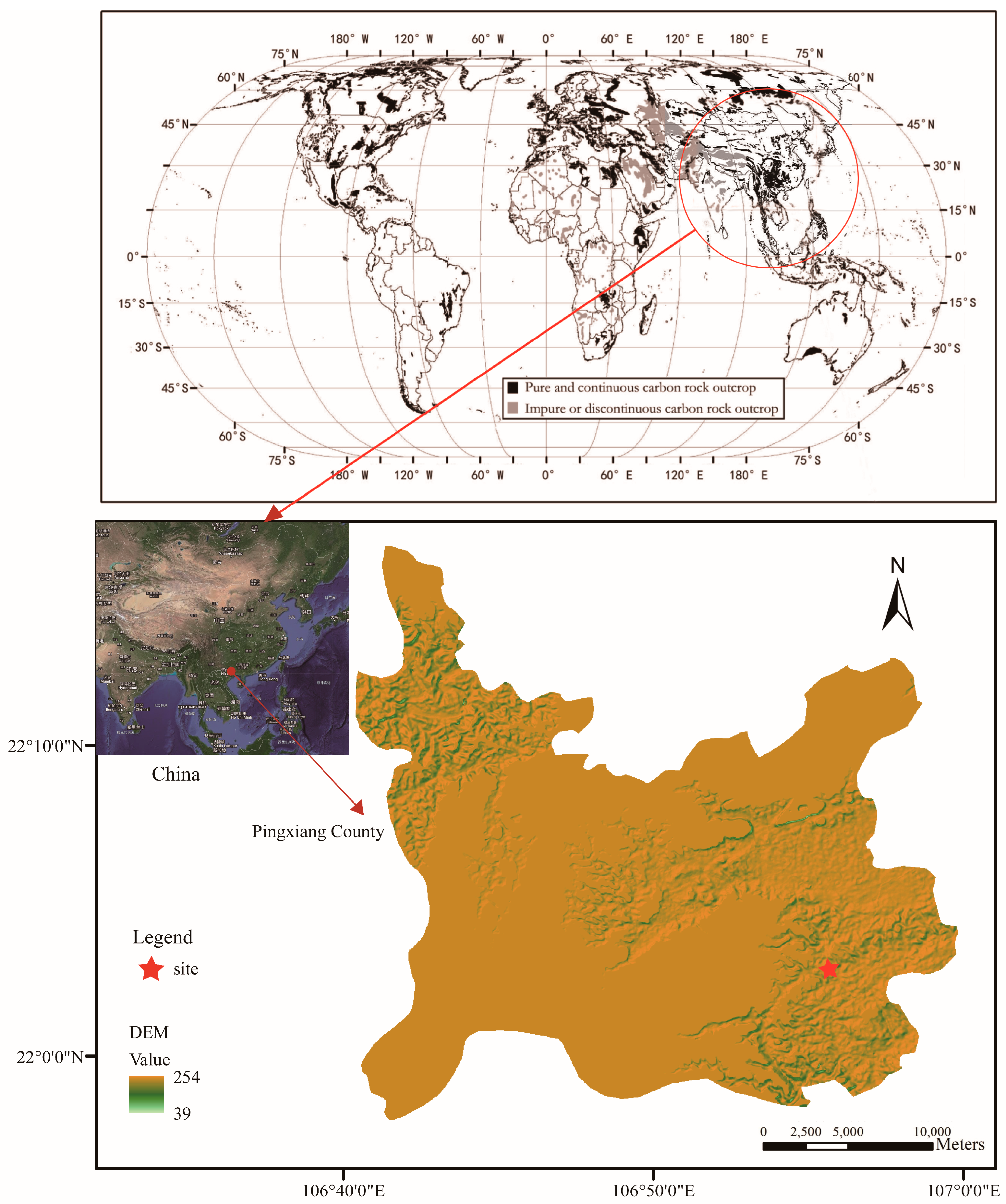
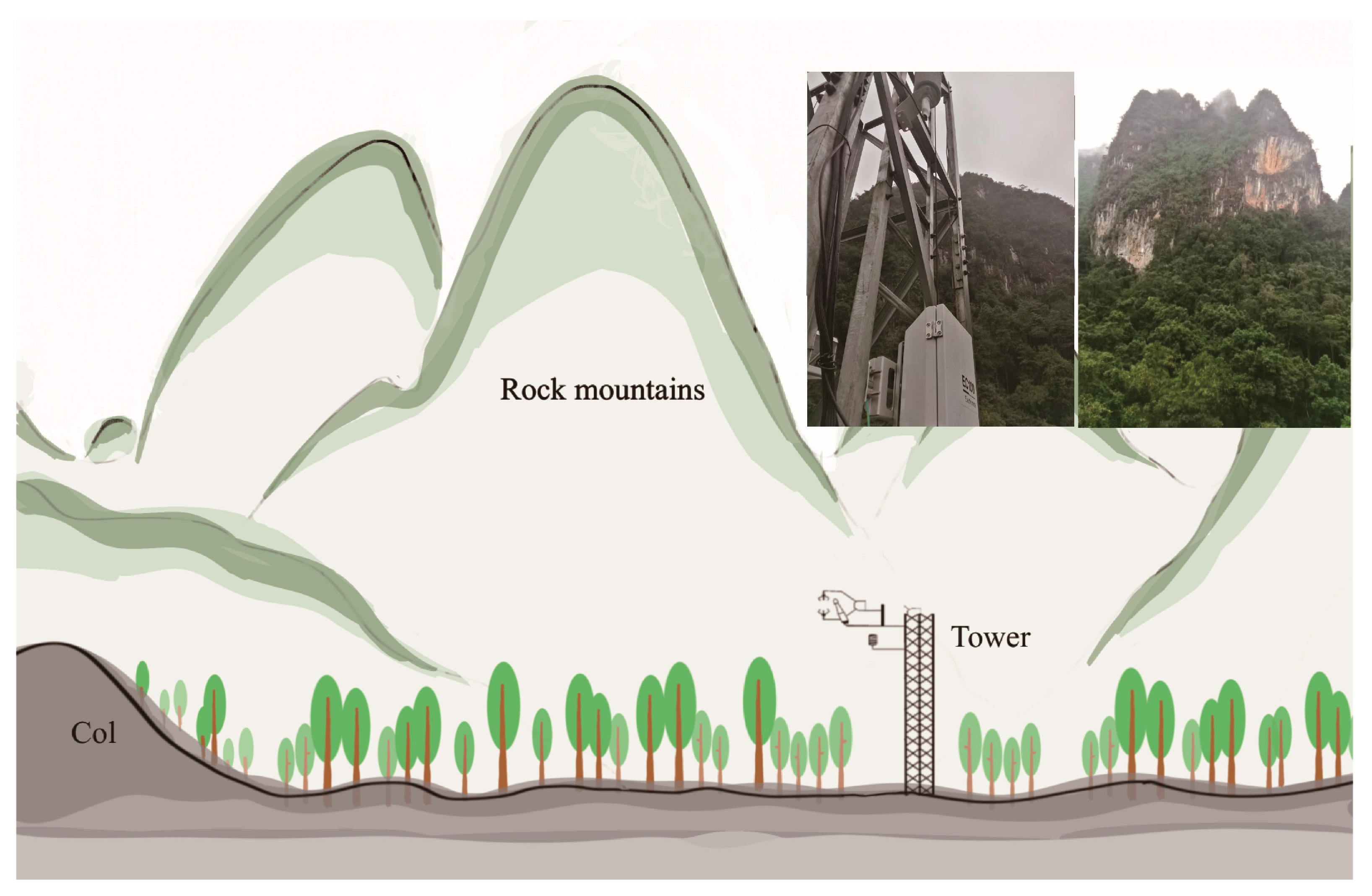
2.1. Site Description

The research was conducted in a seasonal tropical montane rainforest located in Nonggang, Guangxi, China. The flux tower was set up in a valley (106°55′58″ E, 22°2′49″ N), with a slope of 10–15% and an elevation of 190 m (Figure 1). The tower was surrounded by a typical seasonal rainforest of the North Tropical Karst Mountains (Figure 2), dominated by shade-tolerant and moisture-loving tree species, including Saraca dives, Horsfieldia kingii, Ficus hispida and some scattered deciduous tree species [32]. The studied forest is generally primary, and the mean canopy height is about 25 m, with a maximum leaf area index of 4.35 and a mean value of 3.3. The annual net primary productivity of the North Tropical Karst Mountains seasonal rainforest was approximately 11.76 ${\mathrm{t}\mathrm{ha}}^{-1}$. The average annual litterfall from 2013 to 2018 was 4099.44 ${\mathrm{kg}\mathrm{ha}}^{-1}$ [33].

The study area is characterized by a tropical monsoon climate. It is mainly influenced by the southwest monsoon from the northern Indian Ocean during spring and summer, with a prevailing southerly wind and high humidity and rainfall. During summer and autumn, it is mainly affected by the equatorial monsoon, with an easterly wind direction, hot weather and abundant rainfall. During winter and spring, it is mainly influenced by the northeast monsoon of the continental high-pressure system, with an easterly wind direction and relatively low temperatures. The average annual temperature is 22 °C, and the average temperature in the coldest month is above 13 °C. The average annual precipitation is between 1150 mm and 1550 mm, with a maximum of 2043 mm and a minimum of 890 mm. About 76% of the rainfall is concentrated from May to September, and the wet season is prone to waterlogging due to poor drainage. From November to February of the following year, the rainfall is relatively low, with a clear dry and wet season cycle [34].

The terrain is a valley of the karst peak-clustered landform, with high vegetation coverage, a short sunshine duration, an uneven distribution of rocks and a humid environment throughout the year. The soil is continuously distributed with hydromorphic brown lime soil, with a thickness of up to 60 cm. The surface water is scarce in the area, and rainwater is easily lost from underground pipes, leading to geological drought even during the rainy season. The area has abundant underground water channels, many sinkholes, caves and extensive underground streams, forming a complex underground river system. The lowest water level during the dry season (December to February of the following year) is buried 5–25 m deep, and the highest water level during the wet season (May to July) is 0–3 m above the ground.

2.2. Data Collection and Processing

The observation instruments used in this study include a turbulence-related system, a four-component net radiometer and a meteorological observation system. The turbulence-related system is an open-path infrared gas analyzer (IRgaSON, from Campbell Scientific, North Logan, UT, USA) that is integrated with a three-dimensional sonic anemometer to measure in the same space, avoiding high-frequency flux losses when two sensors are measuring in different spaces. Both sensors share an electronic signal processing system, which better coordinates measurement times and eliminates the need for time delay correction. The IRgaSON simultaneously measures CO₂/H₂O, air temperature, atmospheric pressure, three-dimensional wind speed and sonic air temperature at a sampling frequency of 10 Hz.

The radiative components (including downward shortwave radiation, upward shortwave radiation, downward longwave radiation and upward longwave radiation) are measured by a four-component net radiometer (CNR4, from Kipp & Zonen, Delft, Netherlands). The detection system is divided into two parts: the meteorological gradient observation system and the carbon flux and soil observation system. The meteorological gradient observation system includes a data acquisition system (CR1000), a storage system measurement system (CFM100 data storage module, 2 GB memory card), a measurement system (hmp155a temperature and humidity sensor, 52,203 rain gauge, cs106 atmospheric pressure sensor, 05,103 wind speed and direction sensor, csd3 sunshine duration sensor), a power supply system (40 W solar panel, solar charge controller, 24 AH gel battery), auxiliary systems (10 m stainless steel meteorological tower, louvered box), etc. The carbon flux and soil observation system include a data acquisition system (CR3000), a storage system measurement system (CFM100 data storage module, 16 GB memory card), a measurement system (aboveground part: Campbell’s IRgaSON integrated open-path infrared ${\mathrm{CO}}_2/{\mathrm{H}}_2\mathrm{O}$ analyzer, CNR4 radiometer, SI-111 infrared temperature, hmp155a temperature and humidity sensor; underground part: hfp01sc self-calibrating heat flux plate, cs655 soil detection sensor), a power supply system (four 80 W solar panels, two solar charge controllers, two 100 AH gel batteries), auxiliary systems (battery box, bracket), etc.

The steps of data preprocessing and flux calculation include: removing outliers from raw turbulence data [35]; rotating the coordinate axis twice [36]; correcting the time difference between the wind speed and density data using the maximum covariance method; calculating turbulence using the mean trend removal method; calculating half-hourly average flux using Equation (1) and Equation (2); correcting high-frequency and low-frequency flux attenuation [37]; correcting for the density effect of water and heat transfer [38]. The above calculation steps are completed via EddyPro software (version 6.2.0, from LI-COR Biosciences, Lincoln, NE, USA). A half-hourly flux that deviates from the average flux by more than three times the standard deviation is deleted, using a one-day time window. To estimate seasonal and annual cumulative flux, the missing half-hourly flux is interpolated using the monthly average diurnal variation method.

2.3. Methods

2.3.1. Eddy Covariance Method

Water vapor flux, heat flux and momentum flux were continuously measured by an open-path eddy covariance system from 1 January 2019 to 30 June 2020. Air temperature (T) and water vapor density (ρv) were derived from virtual temperature and water vapor measurements. The instrument signals were sampled at 10 Hz, and the average fluxes were calculated and stored at a half-hourly resolution using the covariance between the observed air temperature T, water vapor density ρv and vertical wind speed (U). The fluxes can be calculated as follows:

$$L{E}_{EC}=\lambda \overline{{\rho }_v^{\prime }{U}^{\prime }}$$

(1)

$$H=\rho C_{\mathrm{p}}\overline{T^{\prime }{U}^{\prime }}$$

(2)

where:

• $L{E}_{EC}$ the latent heat flux based on the EC method (W m⁻²);
• ${\rho }_v^{\prime }$ the fluctuation in the water vapor density (kg m⁻³);
• $\lambda$ latent heat of vaporization (J kg⁻¹);
• $U^{\prime }$ the fluctuation in the vertical wind speed (m s⁻¹);
• $H$ the sensible heat flux (W m⁻²);
• $\rho$ the density of dry air (kg m⁻³);
• $C_{\mathrm{p}}$ specific heat capacity of the dry air (1013 J kg⁻¹ K ⁻¹);
• $T^{\prime }$ the fluctuation in the air temperature (°C)

The superscript line indicates the half-time average. The instrument was set up at a height of approximately 33 m and pointed towards the west wind direction, which is the prevailing wind direction. The flux density effect correction was performed using the method described by Webb et al. (1980) [38]. According to Wilczak et al. (2001) [39], three-dimensional rotation and plane-fitting rotation were used to force the average vertical wind speed (U) to be zero and to align the horizontal wind with the mean wind direction.

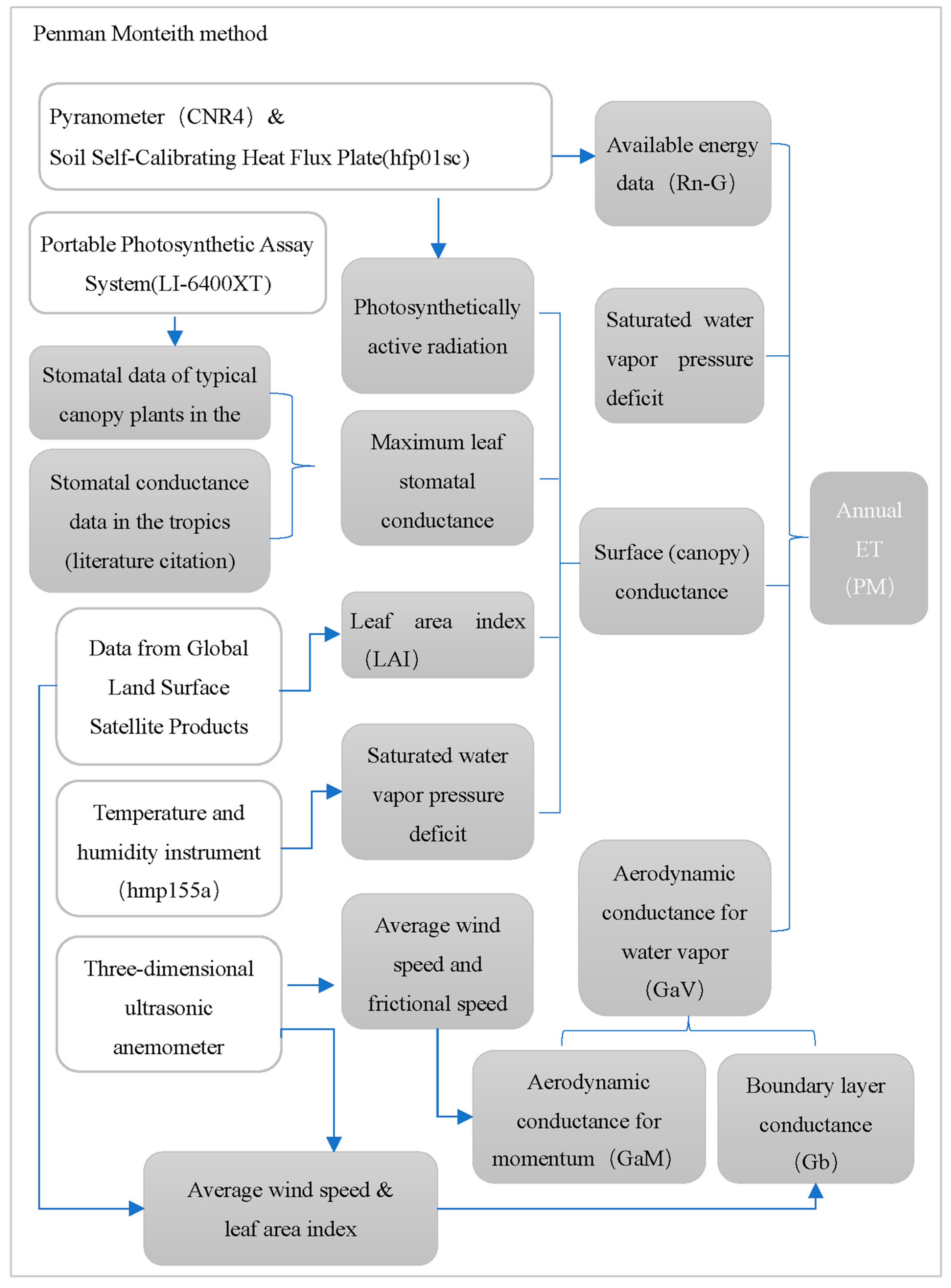
2.3.2. Penman–Monteith Combination Equation

• Calculation Of Evapotranspiration

According to Monteith (1965) [40], the latent heat flux of vegetation can be calculated as follows, and the specific data processing flow chart is shown in Figure 3.

$$L{E}_{PM}=\frac{\mathsf{\Delta }\cdot \left(R_n-G\right)+\rho \cdot C_p\cdot \left(e_s-e_a\right)\cdot G_{aV}}{\mathsf{\Delta }+\gamma \cdot \left(1+G_{aV}/G_s\right)}$$

(3)

$$E{T}_{PM}=\frac{L{E}_{PM}}{\lambda }$$

(4)

where:

• $L{E}_{PM}$ the latent heat flux based on the PM method (W m⁻²);
• $E{T}_{PM}$ evapotranspiration based on the PM method (mm time⁻¹);
• $R_n$ net radiation at the surface (W m⁻²);
• $G$ soil heat flux (W m⁻²);
• $\mathsf{\Delta }$ slope of the saturation vapor pressure–temperature curve (kPa °C⁻¹);
• $\lambda$ latent heat of the vaporization of water (MJ kg⁻¹);
• $\gamma$ psychrometer constant (kPa °C⁻¹);
• $e_s$ saturation vapor pressure (kPa);
• $e_a$ actual vapor pressure (kPa);
• $\left(e_s-e_a\right)$ saturation vapor pressure deficit (kPa);
• $G_{aV}$ aerodynamic conductance for water vapor (m s⁻¹);
• $G_s$ canopy conductance (m s⁻¹).

Please note that $G_s$ and $G_c$ are not equal in reality because $G_s$ depends on the radiation absorbed by the plant canopy, while $G_s$ is a function of the radiation absorbed by both the vegetation canopy and the soil. The measured soil heat flux ($G$) in this study was small, indicating that the radiation absorbed by the soil is small. Therefore, the radiation absorption can be approximated as depending only on the vegetation canopy, and in the subsequent research, $G_s$ and $G_c$ will be replaced by $G_s$.

Slope of saturation vapor pressure curve (Δ)

$$\mathsf{\Delta }=\frac{4098 \left[0.6108\exp \left(\frac{17.27T_a}{T_a+237.3}\right)\right]}{{(T_a+237.3)}^2}$$

(5)

where:

• $\mathsf{\Delta }$ slope of saturation vapor pressure curve at air temperature $T_a$ (kPa °C⁻¹);
• $T_a$ mean air temperature (°C).

$$\gamma =\frac{c_{p}P}{\epsilon \lambda }$$

(6)

where:

• $\gamma$ psychrometric constant (kPa °C⁻¹);
• $P$ atmospheric pressure (kPa);
• $\lambda$ latent heat of vaporization (MJ kg⁻¹);
• $c_p$ air specific heat at constant pressure, 1.013 × 10⁻³ (MJ kg⁻¹ °C⁻¹);
• $\epsilon$ ratio of molecular weight of water vapor/dry air ($\mathsf{\epsilon }=0.622$).

• Calculating the vapor dynamic conductivity

The magnitude of aerodynamic conductivity depends on the aerodynamic characteristics of the underlying surface and atmospheric turbulence intensity. According to Tan et al. (2019) [30], the formula for aerodynamic momentum conductivity is advantageous when the friction velocity u* is available [41], as it overcomes the uncertainties caused by calculating roughness length, displacement height, and non-adiabatic correction function, thus allowing for the calculation of aerodynamic momentum conductivity [42] as follows:

$$G_{\mathrm{aM}}=u_{*}^2/u$$

(7)

where:

• $G_{\mathrm{aM}}$ aerodynamic conductance for momentum (m s⁻¹);
• $u$ the mean wind speed at the reference height (m s⁻¹);
• $u_{*}$ friction velocity at the reference height (m s⁻¹).

According to Tan (2019) [30] and Verma (1989) [43], the boundary layer conductivity $G_b$ is comparable to the aerodynamic momentum conductivity ($G_{\mathrm{aM}}$), and therefore, $G_b$ should not be ignored. According to Wehr et al. (2017) [44], the boundary layer conductivity $G_b$ can be calculated as follows:

$$r_b=2{\left(\frac{Sc}{Pr}\right)}^{\frac{2}{3}}\frac{150}{\mathrm{LAI}}\sqrt{\frac{L}{u}}{\int }_0^1{e}^{0.5\alpha \left(1-\zeta \right)}\varphi \left(\zeta \right)\mathrm{d}\zeta$$

(8)

$$G_b=\frac{1}{r_b}$$

(9)

where $Sc$ is the Schmidt number of water vapor (0.67), $Pr$ is the Prandtl number of air (0.71), $\mathrm{LAI}$ is the leaf area index, $L$ is the characteristic leaf size (0.1 m), $u$ is the mean wind speed at the top of the canopy (m s⁻¹), $\zeta$ is the fraction of height as the height of the canopy top, $\varphi \left(\zeta \right)$ is the vertically normalized light absorption profile such that ${\int }_0^1\varphi \left(\zeta \right)\mathrm{d}\zeta =1$ and $\alpha =4.39-3.97{\mathrm{e}}^{-0.258\times \mathrm{LAI}}$ is the extinction coefficient for the assumed exponential wind profile.

• where:
• $r_{\mathrm{b}}$ boundary layer resistance to water vapor transport (m s⁻¹);
• $G_{\mathrm{b}}$ boundary layer conductance (m s⁻¹);
• $Sc$ Schmidt number for water vapor (0.67);
• $Pr$ Prandtl number for air (0.71);
• $\mathrm{LAI}$ leaf area index (m² m⁻²);
• $L$ characteristic leaf dimension (0.1 m);
• $u$ wind speed at the top of the canopy (m s⁻¹);
• $\zeta$ height as a fraction of canopy top height;
• $\varphi \left(\zeta \right)$ vertical profile of light absorption normalized such that ${\int }_0^1\varphi \left(\zeta \right)\mathrm{d}\zeta =1$;
• $\alpha$ extinction coefficient for the assumed exponential wind profile, $\alpha =4.39-3.97{\mathrm{e}}^{-0.258\times \mathrm{LAI}}$.

Aerodynamic conductance for water vapor ($G_{aV}$) describes the conductance upward from vegetation, which varies with roughness and wind speed and includes momentum aerodynamic conductance ($G_{aM}$) and boundary layer conductance ($G_b$). According to (Thom, 1972; Wesely and Hicks, 1977) [45,46], the aerodynamic conductance for water vapor can be calculated as follows:

$$\frac{1}{G_{\mathrm{aV}}}=\frac{1}{G_{\mathrm{aM}}}+\frac{1}{G_{\mathrm{b}}}$$

(10)

where:

• $G_{\mathrm{aV}}$ aerodynamic conductance for water vapor (m s⁻¹);
• $G_{\mathrm{aM}}$ aerodynamic conductance for momentum (m s⁻¹);
• $G_{\mathrm{b}}$ boundary layer conductance (m s⁻¹).

• Calculation of Canopy Conductance $G_{\mathrm{c}}$

Studies have shown that weather, surface humidity conditions [47] and different vegetation types [48] have an impact on stomatal conductance. In order to obtain more accurate estimates of transpiration simulation, Leuning’s (2008) [48] stomatal conductance model was used, which scales up the leaf-level stomatal conductance model to the canopy level and takes into account the leaf area index and visible radiation flux of the canopy. Meanwhile, water vapor pressure deficit (VPD) is introduced to correct for the influence of the water vapor pressure difference on stomatal conductance. The following equation can be used to calculate stomatal conductance:

$$G_{c\_L}=\frac{g_{smax}}{K_Q}\cdot \frac{1}{1+\left(e_s-e_a\right)/D_{50}}\cdot ln\left(\frac{PAR+Q_{50}}{PAR\cdot exp\left(-K_A\cdot LAI\right)+Q_{50}}\right)$$

(11)

where:

• $G_{c\_L}$ leaf stomatal conductance (m s⁻¹);
• $\left(e_s-e_a\right)$ saturation vapor pressure deficit (kPa);
• $g_{smax}$ the maximum stomatal conductance of leaves at the top of the canopy;
• $D_{50}$ the humidity deficit at which stomatal conductance is half its maximum value, $D_{50}$= 0.7 kpa;
• $Q_{50}$ the visible radiation flux when stomatal conductance is half its maximum value, $Q_{50 }$= 30 W m⁻²;
• $K_Q$ the extinction coefficient for shortwave radiation, $K_{Q }$= 0.6;
• $K_A$ the extinction coefficient for available energy, $K_A$= 0.6;
• PAR the flux density of visible radiation at the top of the canopy (approximately half of incoming solar radiation);

• LAI the leaf area index

Surface conductance ($G_s$, ${\mathrm{m}\mathrm{s}}^{-1}$) is the most commonly used parameter to describe the ability of water vapor to enter the atmosphere via the surface (including soil, canopy space and leaf stomata) [48]. It can be calculated by transforming the observed ${LE}_{EC}$ from the EC method and using the Penman–Monteith equation to obtain $G_{s\_EC}$, i.e.,

$$G_{s\_EC}=\frac{L{E}_{EC}\cdot \gamma \cdot G_{aV}}{\mathsf{\Delta }\cdot \left(R_n-G\right)+\rho \cdot c_p\cdot \left(e_s-e_a\right)\cdot G_{aV}-L{E}_{EC}\cdot \left(\mathsf{\Delta }+\gamma \right)}$$

(12)

where:

• $L{E}_{EC}$ the latent heat flux (W m⁻²);
• $R_n$ net radiation at the surface (W m⁻²);
• $G$ soil heat flux (W m⁻²);
• Δ slope of the saturation vapor pressure–temperature curve (kPa K⁻¹);
• $\gamma$ psychrometer constant (kPa K⁻¹);
• $e_s$ saturation vapor pressure (kPa);
• $e_a$ actual vapor pressure (kPa);
• $\left(e_s-e_a\right)$ saturation vapor pressure deficit (kPa);
• $G_{aV}$ aerodynamic conductance for water vapor (m s⁻¹);
• $G_{sEC}$ surface conductance (m s⁻¹).

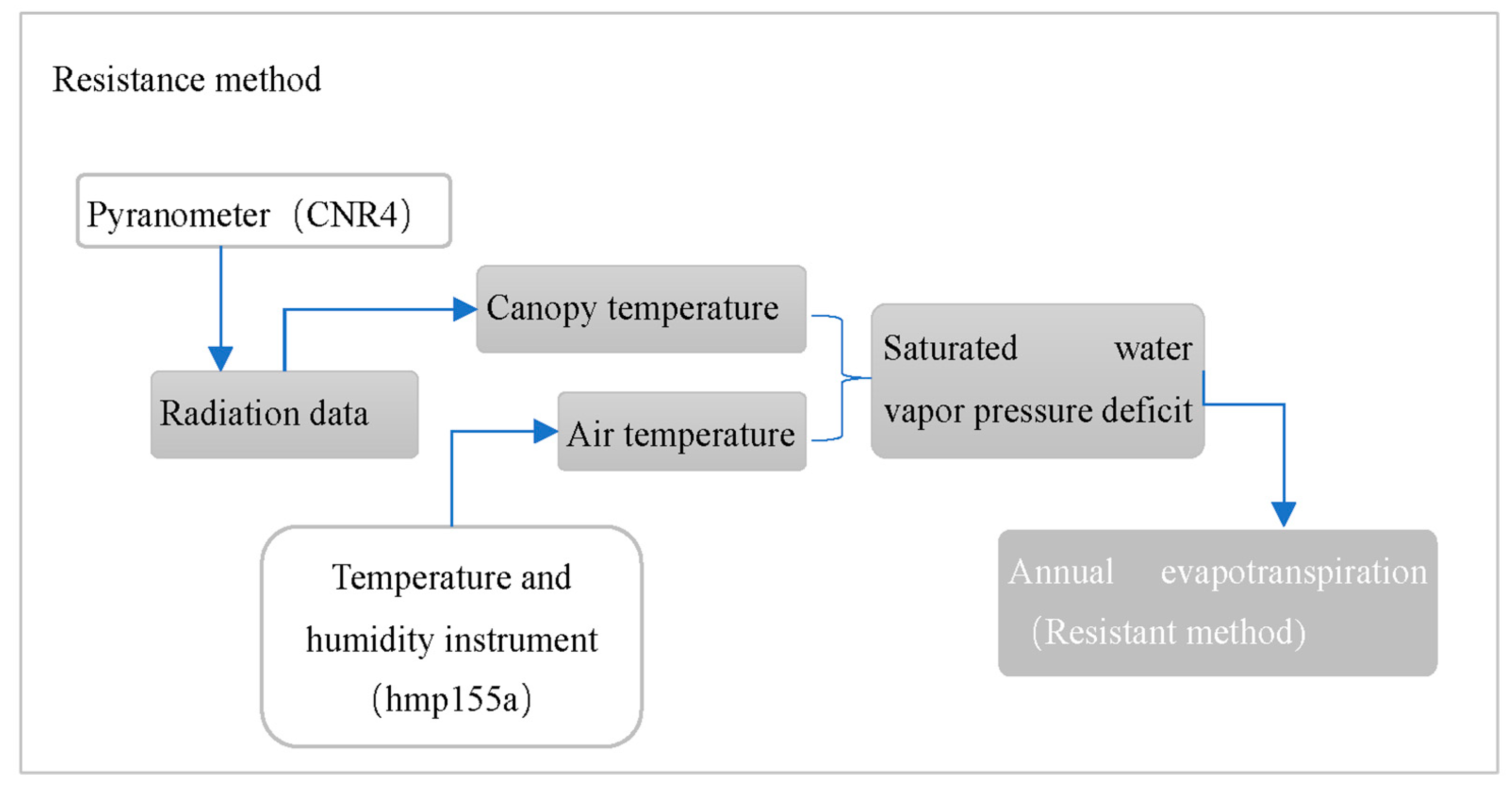
2.3.3. The Resistance Method

The sensible heat ($H_s$) energy on the surface of crops is transferred from the air to the crop surface or from the crop surface to the air, and this transfer can be described by a similar equation [49]:

$$H_{res}=\rho C_p\left(T_s-T_a\right)G_{aV}$$

(13)

where:

• $\rho$ mean air density at constant pressure (kg m⁻³);
• $C_p$ air-specific heat at constant pressure (MJ kg⁻¹ °C⁻¹);
• $e_s$ saturation vapor pressure (kPa);
• $e_a$ actual vapor pressure (kPa);
• ($e_s$ − $e_a$) saturation vapor pressure deficit (kPa);
• $G_{aV}$ aerodynamic resistance (m s⁻¹);
• $T_s$ the canopy temperature (K);
• $T_a$ the air temperature (°C).

In this study, the canopy temperature was not directly measured but was obtained through the inversion of radiative data. According to Stefan–Boltzmann’s law [50,51], the higher the temperature of an object, the more total energy it radiates outward, and the radiative energy E it radiates per unit area in unit time can be expressed as:

$$E=\epsilon \sigma T^4$$

(14)

where:

• E upward long-wave radiation (W ${\mathrm{m}}^{-2}$);
• ε the emissivity of the object, which is a value between 0 and 1 and is determined by the surface properties of the object;
• σ the Stefan–Boltzmann constant, σ = 5.67 × ${10}^{-8}$ W/(${\mathrm{m}}^2$·${\mathrm{K}}^4$);
• $T$ the canopy temperature (K).

The energy dissipated by the latent heat (LE) on the surface of crops is determined by four microclimate factors (the effective energy of net radiation minus soil heat flux (R_n-G), air temperature (T_a), air vapor pressure deficit (VPD) and wind speed or air diffusivity (G_a)) and a physiological factor (crop conductance (G_c)). According to Brown and Norman (1973) [49], the dependence of LE on these parameters can be expressed by the following equation, and the specific data processing flow chart is shown in Figure 4:

$$L{E}_{res}=\frac{\rho C_p}{\gamma }\frac{\left(e_s-e_a\right)}{\frac{1}{G_{aV}}+\frac{1}{G_c}}$$

(15)

where:

• $\rho$ mean air density at constant pressure (kg m⁻³);
• $C_p$ air-specific heat at constant pressure (MJ kg⁻¹ °C⁻¹);
• $e_s$ saturation vapor pressure (kPa);
• $e_a$ actual vapor pressure (kPa);
• $\left(e_s-e_a\right)$ saturation vapor pressure deficit (kPa);
• $\gamma$ psychrometric constant (kPa °C⁻¹);
• $G_c$ canopy resistance (m s⁻¹);
• $G_{aV}$ aerodynamic resistance (m s⁻¹).

2.3.4. Potential Evapotranspiration

The potential evapotranspiration calculated by the Penman equation can be described as follows, with the surface conductance (G_c) set to nearly infinity:

$$\lambda PE=\frac{\mathsf{\Delta }\left(R_n-G\right)+\rho c_p\left(e_s-e_a\right)G_{aV}}{\mathsf{\Delta }+\gamma \left(1+\frac{G_{aV}}{G_c}\right)}$$

(16)

where:

• $\lambda$ latent heat of vaporization of water (MJ kg⁻¹);
• $PE$ potential evapotranspiration (mm day⁻¹);
• $R_n$ net radiation at the crop surface (MJ m⁻² day⁻¹);
• $G$ soil heat flux (MJ m⁻² day⁻¹);
• $\rho$ mean air density at constant pressure (kg m⁻³);
• $c_p$ air-specific heat at constant pressure (MJ kg⁻¹ °C⁻¹);
• $e_s$ saturation vapor pressure (kPa);
• $e_a$ actual vapor pressure (kPa);
• $\left(e_s-e_a\right)$ saturation vapor pressure deficit (kPa);
• $\mathsf{\Delta }$ slope vapor pressure curve (kPa °C⁻¹);
• $\gamma$ psychrometric constant (kPa °C⁻¹);
• $G_c$ canopy resistance (m s⁻¹);
• $G_{aV}$ aerodynamic resistance (m s⁻¹).

2.3.5. Reference Evapotranspiration FAO56

The Penman–Monteith method of the Food and Agriculture Organization provides estimates of reference evapotranspiration (ET_o) for a reference surface. This method defines the reference surface based on the following assumptions: “a crop height of 0.12 m, a constant surface resistance of 70 s ${\mathrm{m}}^{-1}$ and an albedo of 0.23” [52].

$$E{T}_o=\frac{0.408\mathsf{\Delta }\left(R_n-G\right)+\gamma \frac{900}{T_a+273}{u}_2\left(e_s-e_a\right)}{\mathsf{\Delta }+\gamma \left(1+0.34u_2\right)}$$

(17)

where:

• $E{T}_o$ reference evapotranspiration (mm day⁻¹);
• $R_n$ net radiation at the crop surface (MJ m⁻² day⁻¹);
• $G$ soil heat flux density (MJ m⁻² day⁻¹);
• $T_a$ mean daily air temperature at 2 m height (m s⁻¹);
• $u_2$ wind speed at 2 m height (m s⁻¹);
• $e_s$ saturation vapor pressure (kPa);
• $e_a$ actual vapor pressure (kPa);
• $e_s-e_a$ saturation vapor pressure deficit (kPa);
• Δ slope vapor pressure curve (kPa °C⁻¹);
• γ psychrometric constant (kPa °C⁻¹).

2.4. Energy Balance Calculation

Energy balance closure is a formula of the first law of thermodynamics which requires the sum of latent heat flux (LE) and sensible heat flux (H) to be equal to all other energy sinks and sources. The energy balance equation [53] is generally expressed as:

$$LE+H=R_n-G-S-Q$$

(18)

where $R_n$ is the net radiation at the ecosystem canopy (W·m⁻²), which is the ultimate source of energy required for ecosystem physiological processes. When the ecosystem gains energy, $R_n$ is positive, and when the energy is released from the ecosystem, $R_n$ is negative; $G$ is the heat flux into the soil matrix, $S$ is the storage of heat between the sonic anemometer and the soil surface and $Q$ is the sum of all additional energy sources and sinks (mainly referring to the energy consumed by ecosystem vegetation photosynthesis). In general, $S$ and $Q$ are small terms that are ignored. Therefore, the flux balance can be simplified as:

$$LE+H=R_n-G$$

(19)

In the equation above, the right-hand side represents available energy and the left-hand side represents the standard turbulent flux. Imbalances between the two sides may indicate inaccurate estimates of scalar fluxes. However, in reality, surface energy fluxes ($R_n-G$) are often (but not always) underestimated by around 10–30% relative to available energy ($LE+H$) [54,55,56]. Even on flat, uniform surfaces with short vegetation, such imbalances often exist, although to a lesser extent [21,57,58].

The energy balance ratio (EBR) is calculated as follows:

$$EBR=\left(LE+H\right)/\left(R_n-G\right)$$

(20)

$$L{E}_{cor}=LE\left(R_n-G\right)/\left(LE+H\right)$$

(21)

where R_n is the net radiation of the ecosystem canopy, LE is the latent heat flux (W·m⁻²), H is the sensible heat flux (W·m⁻²), G is the soil heat flux (W·m⁻²) and $L{E}_{cor}$ is the corrected latent heat flux (W·m⁻²).

3. Results

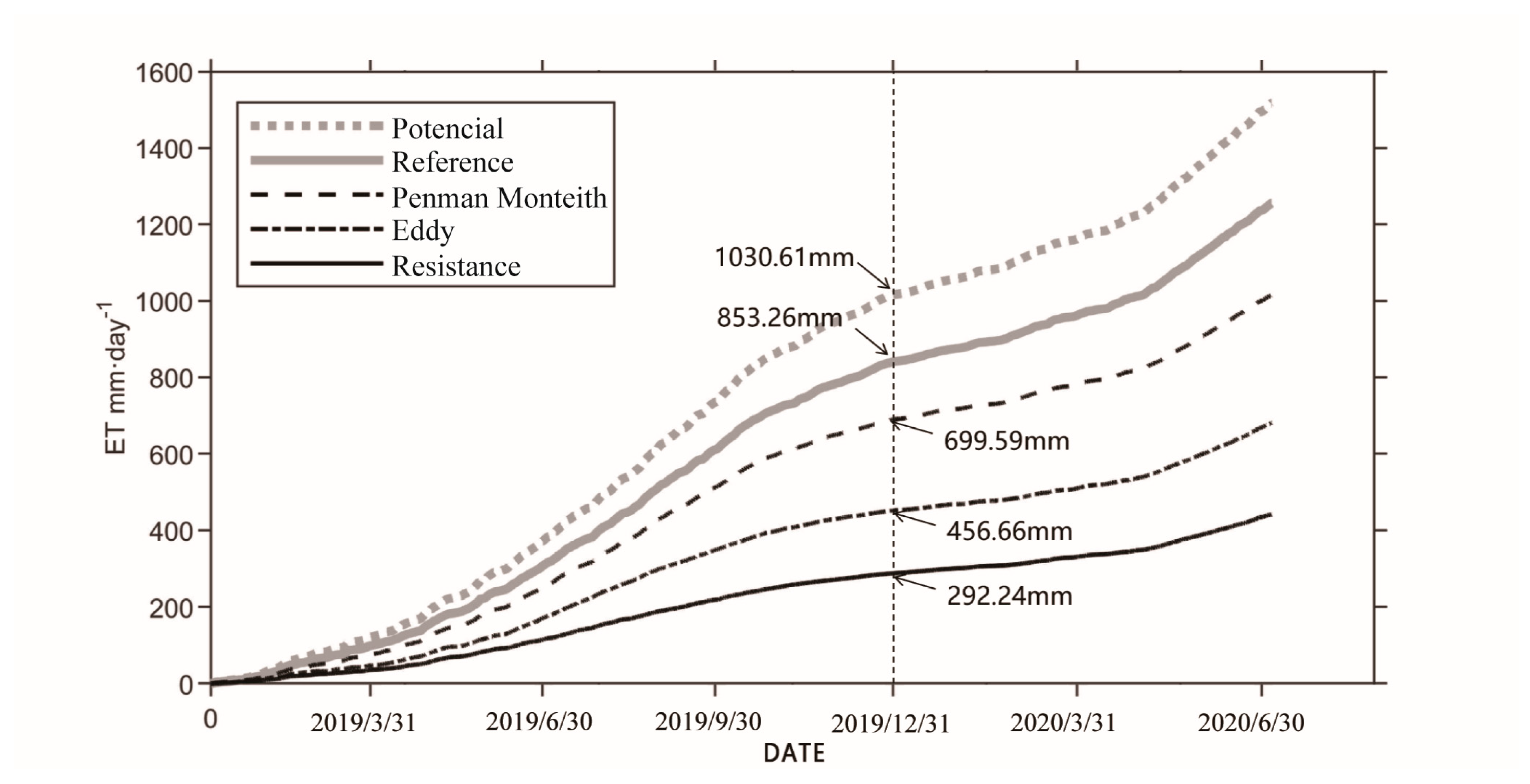
3.1. Comparison of Independent Methods for Estimating Evapotranspiration

The estimated annual evapotranspiration based on three different methods is shown in Figure 5. The annual evapotranspiration of the Nonggang karst forest was 456.66 mm (eddy covariance method), 292.24 mm (resistance method) and 699.59 mm (Penman–Monteith method). There were differences in the annual evapotranspiration values among the three methods, but all were lower than the reference evapotranspiration (853.26 mm year⁻¹) and potential evapotranspiration (1030.61 mm year⁻¹).

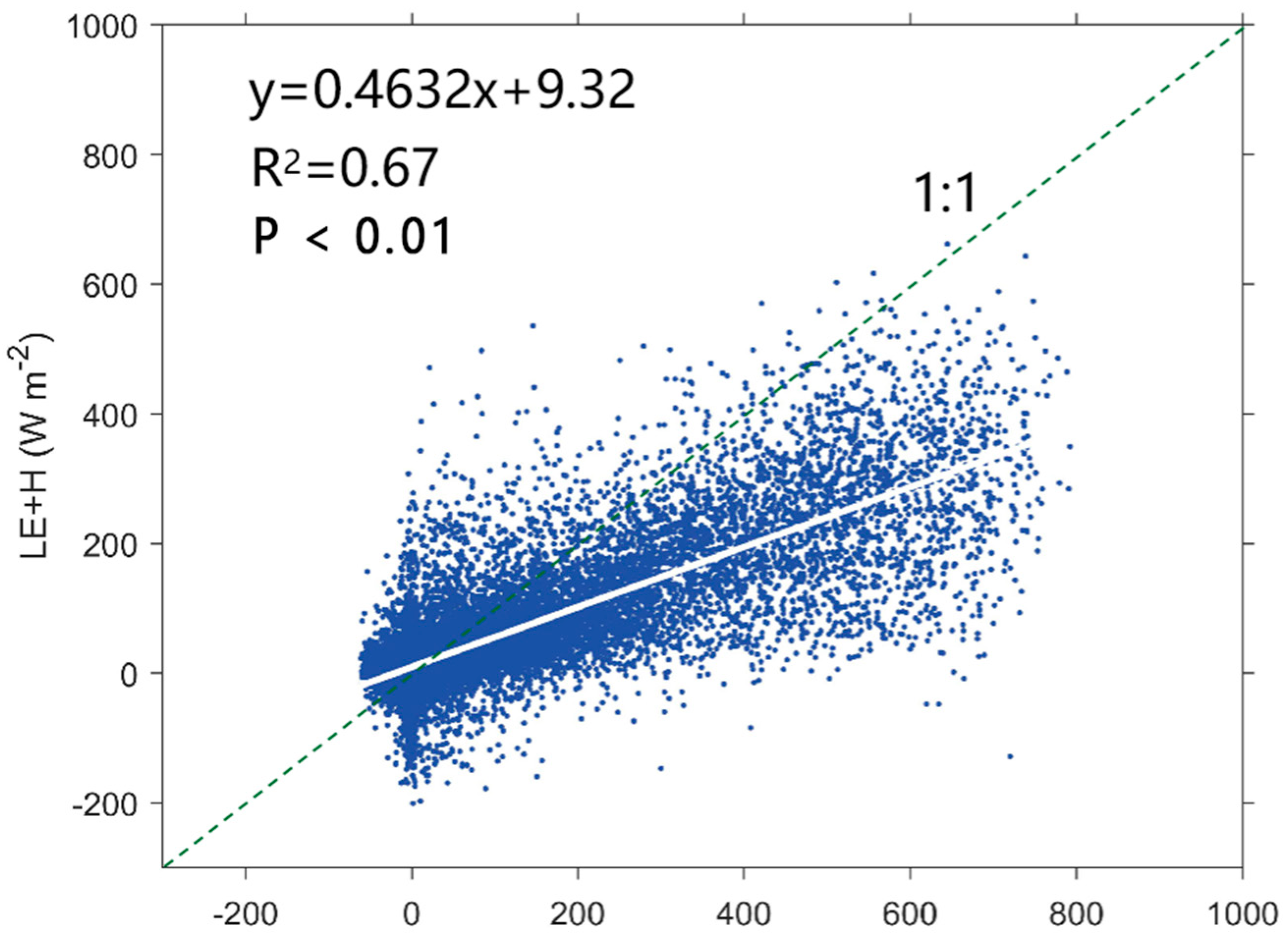
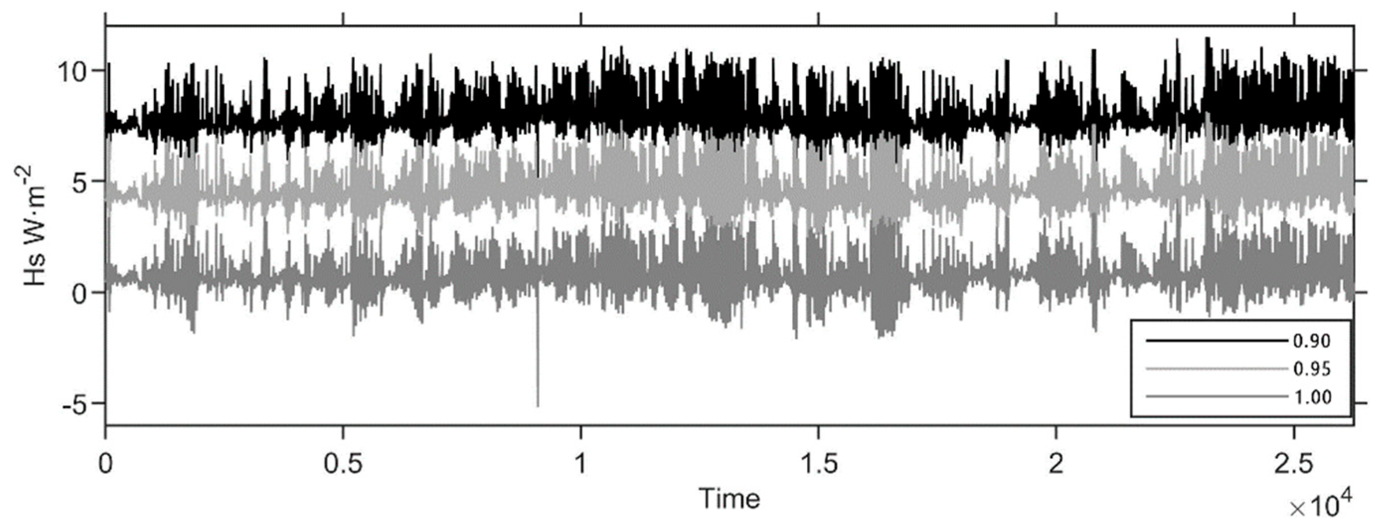
3.1.1. Energy Closure Analysis (EC Method)

To confirm the reliability of the observed data, we calculated the energy closure. The results showed that the energy closure in the study area was 46% (Figure 6). At the half-hourly time step, the regression slope between turbulent fluxes (LE + H) and available energy (R_n-G) was 0.46, the intercept was 9.32 and the correlation coefficient was 0.67. The calculation results in Section 2 showed that the turbulent flux-based energy closure at the site was low, which was below the reasonable range value previously reported (55~80%). To address this issue, we conducted an energy closure correction assuming that both latent and sensible heat fluxes were consistently underestimated (Twine et al., 2000) and adjusted the Bowen ratio to quantify the systematic underestimation of turbulent fluxes. This method has been supported by airborne measurements [59].

3.1.2. Eddy Covariance Method

The estimated annual evapotranspiration based on different energy closure is shown in Figure 7. The annual evapotranspiration in 2019 after correction based on 100% energy closure is 915.03 mm, which is higher than the reference evapotranspiration of 853.26 mm and lower than the latent heat evapotranspiration of 1030.61 mm. The estimated annual evapotranspiration after a 100% energy closure correction was found to be unreasonably high, even exceeding the reference evapotranspiration, indicating that the corrected estimate of annual evapotranspiration is not reasonable.

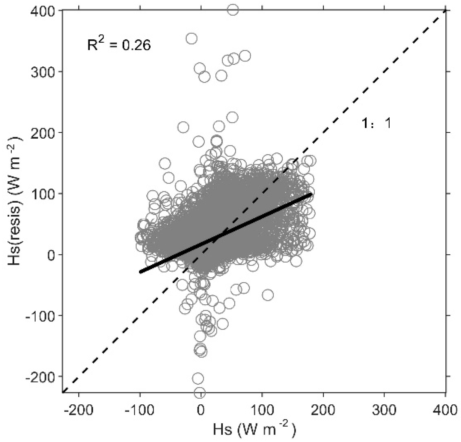
3.1.3. Comparison between Eddy Covariance and Resistance Methods

Due to the lack of canopy temperature data, the temperature data used in the resistance method of this study were calculated by a radiometer. To ensure the reliability of the resistance method data, we evaluated the effect of emissivity (a key parameter in the calculation process) on the sensible heat flux. The half-hourly mean sensible heat flux under different emissivity values (Figure 8) shows that the emissivity value has a significant impact on the sensible heat flux. Considering that most studies have set emissivity to a constant value of 0.9 based on experimental support, we believe that an emissivity value of 0.9 is relatively safe.

Figure 5 shows that the estimated annual evapotranspiration obtained by the resistance method is nearly 164.24 mm (36%), which is lower than that obtained by the eddy covariance method. As mentioned in Section 2.2, the resistance method calculates sensible heat flux and latent heat flux based on temperature data (canopy temperature and air temperature), while the eddy covariance method obtains sensible and latent heat data through high-frequency instruments such as sonic anemometers and gas analyzers. The temperature data for the resistance method are retrieved through radiometers, and this is relatively independent of the eddy covariance method. The calculated results have a significant difference compared to the values obtained by the eddy covariance method, with a correlation coefficient $R^2$ of only 0.26 (Figure 9). The sensible heat flux obtained by the resistance method is significantly lower than that obtained by the EC method, but the seasonal trend is consistent (Figure 10). Comparing the resistance method with the EC method, it was found that not only is the annual evapotranspiration (ET) lower in the EC method, but the sensible heat flux is also lower, indicating that the resistivity method has lower energy closure than the EC method, suggesting that this method is not suitable for use in karst forests.

3.1.4. Comparing the Eddy Covariance and PM Method

Based on Figure 11, the annual estimated transpiration rate simulated by the PM method is higher than the one measured by the eddy covariance method when the g_smax values are 0.004 m s⁻¹, 0.006 m s⁻¹ and 0.007 m s⁻¹. On the other hand, when g_smax is 0.001 m s⁻¹, the PM method produces a lower estimate than the one measured by the eddy covariance method. Among them, 0.001 m s⁻¹, 0.004 m s⁻¹ and 0.007 m s⁻¹ are the maximum stomatal conductance values of the key tree species in the forest canopy (namely, Prunus salicina, Osmunda japonica and Ficus altissima, respectively) determined by the LI-6400XT portable photosynthesis system in the field [60], and 0.006 m s⁻¹ is the average value of the maximum single-leaf stomatal conductance (g_smax) dataset in a tropical rainforest from Kelliher (1995) [61]. All the maximum leaf stomatal conductance values are within the range of 0.0029 m s⁻¹ to 0.0093 m s⁻¹, which is the maximum stomatal conductance range of tropical forest leaves mentioned in the study of Kelliher and Leuning et al. [61].

Surface conductance is the most difficult parameter to quantify in the Penman–Monteith equation, as it depends on plant physiological behavior rather than physical properties and is subject to greater variability than other model parameters. To make the model’s evapotranspiration predictions more accurate, this parameter must be accurately specified. In order to ensure the performance of the stomatal conductance model, we first conducted a sensitivity analysis of the two parameters of solar radiation when stomatal conductance is half its maximum value (${\mathrm{D}}_{50}$) and atmospheric humidity deficit (${\mathrm{Q}}_{50}$). As shown in Figure 12, the effect of parameter changes on model performance is very small when ${\mathrm{D}}_{50}$ is greater than 0.5 kPa and ${\mathrm{Q}}_{50}$ is greater than or equal to 30 μmol ${\mathrm{m}}^{-2}$${\mathrm{s}}^{-1}$. In addition, according to Leuning’s simple stomatal model [62], we found that surface conductance varies with biotic factors in the equation, except for the leaf area index, and the most difficult parameter to determine is the maximum single-leaf stomatal conductance. Therefore, it is necessary to accurately specify the selection of the maximum single-leaf stomatal conductance (g_smax) parameter. The surface conductance measured by the eddy covariance method does not have the same sampling problem, as the flux represents the evaporation of all vegetation in a large number of counter-flowing air currents.

As shown in Figure 13, annual evapotranspiration is relatively sensitive to the selection of the maximum leaf stomatal conductance parameter, especially when g_smax is less than 0.02 m s⁻¹, and evapotranspiration reaches a steady state of around 1000 mm. We also found that when g_smax is 0.0025 m s⁻¹, the annual evapotranspiration estimated by the two independent methods tends to converge (456 mm). When g_smax is less than 0.0025 m s⁻¹, the evapotranspiration estimated by the PM method is lower than that measured by the eddy covariance method, and vice versa. When the maximum leaf stomatal conductance (g_smax = 0.018 m s⁻¹) cited in the estimation of evapotranspiration in the Southwest Karst region is introduced, the annual evapotranspiration reaches 901.86 mm.

3.2. Surface Conductance Analysis

To verify the reliability of the canopy conductance parameter, we used eddy covariance to invert canopy conductance (as shown in Figure 14). The results were similar to those of most forests of the same type, and the canopy conductance parameter selected in the Penman–Monteith–Leuning method was between 0 and 0.01 ${\mathrm{m}\mathrm{s}}^{-1}$. The surface conductance exhibited a sudden increase in the morning, reached its maximum around 11 a.m. and then gradually decreased. Both methods obtained the maximum surface conductance in August in the morning. The range of canopy conductance values obtained by the two independent methods was consistent with the seasonal pattern, which to some extent indicated the reliability of the transpiration results. These findings contribute to a better understanding of forest water use and provide a reference for the estimation of water balance and forest management in similar ecosystems.

The value of $G_C$ in the Food and Agriculture Organization’s reference evapotranspiration model is an empirical value based on experiments, and this canopy conductance is an upper limit value for forest canopies determined by the characteristics of the reference crop. After comparing the numerical range and seasonal pattern of the canopy conductance, we compared the annual average values of the two methods of obtaining canopy conductance with the $G_C$ canopy conductance (fixed value of 1/70 ${\mathrm{m}\mathrm{s}}^{-1}$) of the reference crop in order to further confirm the reliability of the estimated annual transpiration. The comparison results showed that the mean canopy conductance obtained by the eddy covariance inversion method was 0.0022 ${\mathrm{m}\mathrm{s}}^{-1}$, and the mean canopy conductance obtained by the Penman–Monteith–Leuning method was 0.0025 ${\mathrm{m}\mathrm{s}}^{-1}$, both of which were less than 1/70 ${\mathrm{m}\mathrm{s}}^{-1}$. Based on the above analysis, we believe that the canopy conductance obtained by the two methods is reliable and can further judge the reliability of the annual transpiration estimation based on the canopy conductance.

4. Discussion

According to the analysis of the results above, the conclusions obtained from the three methods for estimating annual evapotranspiration are inconsistent, indicating uncertainties in the estimates from different independent methods. The EC method cannot ignore the problem of low energy closure. In areas with complex topography, low energy closure is common, and currently, the energy closure rate at many global sites is usually only around 80% [20,53,63]. Some estimates agree with actual evapotranspiration after energy closure correction, while others remain consistent with actual evapotranspiration even without energy closure correction. Currently, it is not clear to what extent the remaining differences between the EC method and the other two methods are due to insufficient energy balance correction or to different spatiotemporal scales of measurement concepts among the different methods. However, our results clearly indicate that if the lack of energy balance closure is adjusted according to the Bowen ratio energy balance correction method [21] using a 100% correction rate, it may lead to unreliable estimates of evapotranspiration. This also demonstrates that the scalar similarity between sensible heat flux and latent heat flux is not applicable at the scale of our study site. Therefore, we speculate that, in some cases, energy closure correction may not be necessary, or it may be possible to correct based on an 80% energy closure rate, but the specific correction rate for energy closure is currently unclear and requires further discussion in future studies.

Some studies have compared the estimation of evapotranspiration using the EC and PM methods. Siedlecki et al. (2022) compared the evapotranspiration of the FAO PM method and the EC method in farmland ecosystems, and the results showed that they were quite consistent, especially during periods of high precipitation and full development [64]. Pauwels et al. (2006) compared the results of evapotranspiration obtained by the EC and PM methods and found that the correlation between the two methods at a half-hour time scale was nearly 86%, indicating a high level of consistency [65]. Other studies have found that the evapotranspiration estimated by the PM method exceeded that estimated by the EC method by 131% [66]. This suggests that the PM method has a high level of credibility in evaluating actual evapotranspiration, but the choice of different maximum stomatal conductance is still a key factor affecting the accuracy of PM method results. Shi et al. overestimated the actual evapotranspiration by 131% by selecting the maximum stomatal conductance (0.0056 m s⁻¹) for a temperate mixed forest [66], while Pauwels et al. (2006) obtained consistent results for a wet grassland by using a fixed surface conductance of 1/70 m s⁻¹ for the PM method [65]. The careful selection of maximum stomatal conductance can greatly increase the credibility of PM method evapotranspiration estimates.

According to the sensitivity analysis of annual transpiration to maximum stomatal conductance, when g_smax is less than 0.018 m s⁻¹, the different values of maximum stomatal conductance have a significant impact on it, indicating that a more conservative selection of maximum stomatal conductance is required to obtain relatively accurate estimates of annual transpiration. First, we evaluated the canopy conductance obtained by the EC method and the PM method based on the fixed value of the surface conductance of reference evapotranspiration, and the results showed that both were lower than 1/70 m s⁻¹, indicating that the value of maximum stomatal conductance is credible. Therefore, we obtained the range of maximum stomatal conductance within the allowable limits. Studies have shown that there are significant differences in stomatal conductance among different vegetation types [2]. Jiang et al. used the Breathing Earth System Simulator (BESS) model to calculate ET, and the results showed that distinguishing between C3 and C4 plants in the model improved accuracy compared to not distinguishing between vegetation types [3]. To obtain relatively accurate parameters of canopy conductance, we believe that selecting the maximum leaf stomatal conductance of a key tree species in the forest where the eddy covariance station is located can provide a relatively accurate estimate of annual transpiration. Although the stomatal characteristic data are based on literature research, the actual sampling points of the data are located within the study site area, without temporal and spatial differences, which can provide relatively accurate results. Therefore, in this study, we tend to believe that 0.006 ${\mathrm{m}\mathrm{s}}^{-1}$ as the maximum single-leaf stomatal conductance (g_smax) for PML method applications is relatively reasonable. However, the following issue still exists: in complex vegetation canopies, some tree crowns may extend beyond the general horizontal of the canopy, and this variability may cause problems when sampling vegetation to obtain representative stomatal conductance. To use stomatal conductance measurements to estimate transpiration, representative samples are needed in both the horizontal and vertical directions [67]. The maximum leaf stomatal conductance of a single tree species used in this study cannot represent the comprehensive characteristics of all species. It is critical to find the maximum leaf stomatal conductance that can represent all species, and this issue may need to be further explored in future studies.

In principle, Gs can be calculated by the direct measurement of surface temperature using the flux gradient equation (resistance method). However, this method is rarely used to calculate Gs because the Gs value obtained is unreliable due to differences in the projection area of surface temperature and evaporation flux measurement, as well as uneven surface temperature [68].

Compared with the EC (eddy covariance) method, the annual evapotranspiration estimated by the resistance method is much lower (nearly 36% lower than that of EC method). In our study, we compared the effects of different emissivity on the sensible heat flux data and found that the sensible heat flux varied greatly with different emissivity. We used a relatively conservative emissivity parameter to ensure the reliability of the sensible heat flux data. Additionally, the study results showed that the sensible heat flux obtained from radiative data (resistance method) had poor correlation (26%) and large differences in quantity compared to the sensible heat flux directly measured by the EC method. The former was significantly smaller than the latter, but the seasonal trends were very consistent. The consistent seasonal trends indicated that the radiative data and temperature data obtained by micro-meteorological measurements had consistent seasonal trends, indicating the reliability of the radiative data. Furthermore, the sensible heat flux and latent heat flux obtained by the resistance method were both smaller than those obtained by the EC method, indicating that the effective energy (LE + Hs) obtained by the resistance method was lower than that obtained by the EC method, and the energy closure was lower, which greatly reduced its reliability. This is likely due to the fact that the resistance method may have caused larger errors as a result of differences in the projection area of surface temperature and evaporation flux measurements, as indicated by previous studies [49]. While the resistance method has its advantages in terms of simplicity and ease of use, caution must be exercised when interpreting its results and considering its applicability to different environments and conditions. Additional research is needed to further investigate the accuracy and limitations of the resistance method and to develop more robust and reliable methods for estimating evapotranspiration in various settings.

In summary, we believe that the annual evapotranspiration estimates obtained using the Penman–Monteith equation are relatively reliable among the three independent methods. Although there is uncertainty in the parameterization of canopy conductance, the annual evapotranspiration calculated by the PM method is between the EC method and reference evapotranspiration, with values of 596.42 mm (g_smax = 0.004 ${\mathrm{m}\mathrm{s}}^{-1}$), 699.59 mm (g_smax = 0.006 ${\mathrm{m}\mathrm{s}}^{-1}$) and 736.90 mm (g_smax = 0.0047 ${\mathrm{m}\mathrm{s}}^{-1}$), respectively, and is more reliable than the estimates obtained by the other independent methods.

5. Conclusions

(1) The annual estimates of evapotranspiration obtained by three independent methods (eddy covariance, resistance method and Penman–Monteith) were inconsistent, with values of 456.66 mm (eddy covariance), 292.24 mm (resistance method) and 699.59 mm (Penman–Monteith method, with g_smax = 0.006 ${\mathrm{m}\mathrm{s}}^{-1}$). All three methods underestimated annual evapotranspiration compared to reference evapotranspiration (853.26 mm year⁻¹) and potential evapotranspiration (1030.61 mm year⁻¹), which increased the credibility of the results.

(2) The energy balance closure problem exists in the eddy covariance method, with an annual closure of 46%. The annual estimate of evapotranspiration after energy correction was 915.03 mm, which was higher than the reference evapotranspiration (853.26 mm), so we considered the corrected annual estimates of evapotranspiration to be unreasonable. In the future, multiple flux towers will be used for monitoring and combined with high-spatial-resolution lidar and airborne measurements to achieve the intersection of the spatiotemporal scale and independent measurement methods, explore the potential reasons for the lack of energy closure using the eddy covariance method in typical karst geomorphological forests, accurately assess the actual evapotranspiration level in karst areas and promote the sustainable management of regional and global water resources.

(3) In this study, we consider that 0.006 ${\mathrm{m}\mathrm{s}}^{-1}$ as the maximum single-leaf stomatal conductance ($g_{smax}$) for applying the PM method is relatively reasonable. This value considers the field sampling data in the study area and is close to the average value of the maximum single-leaf stomatal conductance ($g_{smax}$) dataset for tropical rainforests mentioned by Kelliher (1995) [61]. The selection of different maximum stomatal conductance parameters has a significant impact on the annual estimate of evapotranspiration by using the PM method. In future studies, we recommend combining multiple measurement methods and scaling methods to obtain more accurate canopy conductance parameters.

(4) Considering the EC method as the lower limit (456.66 mm), the reference evapotranspiration as the upper limit (853.26 mm) and the specific vegetation in the study area, the estimated annual evapotranspiration of the primary forest in the Nonggang karst area of Guangxi (PM method) falls within the range of 596.42 mm to 736.90 mm, which is relatively reasonable.

References

1. Bonacci, O.; Pipan, T.; Culver, D.C. A framework for karst ecohydrology. Environ. Geol. 2009, 56, 891–900. [Google Scholar] [CrossRef]
2. Ford, D.; Williams, P.D. Karst Hydrogeology and Geomorphology; John Wiley & Sons: Hoboken, NJ, USA, 2007. [Google Scholar]
3. Wang, K.; Zhang, C.; Chen, H.; Yue, Y.; Zhang, W.; Zhang, M.; Qi, X.; Fu, Z. Karst landscapes of China: Patterns, ecosystem processes and services. Landsc. Ecol. 2019, 34, 2743–2763. [Google Scholar] [CrossRef]
4. Ma, N.; Szilagyi, J.; Zhang, Y. Calibration-free complementary relationship estimates terrestrial evapotranspiration globally. Water Resour. Res. 2021, 57, e2021WR029691. [Google Scholar] [CrossRef]
5. Zhao, M.; Liu, Y.; Konings, A.G. Evapotranspiration frequently increases during droughts. Nat. Clim. Chang. 2022, 12, 1024–1030. [Google Scholar] [CrossRef]
6. Aubinet, M.; Vesala, T.; Papale, D. Eddy Covariance: A practical Guide to Measurement and Data Analysis; Springer Science & Business Media: Berlin, Germany, 2012. [Google Scholar]
7. Jaeger, L.; Kessler, A. Twenty Years of Heat and Water Balance Climatology at the Hartheim Pine Forest, Germany. Agric. For. Meteorol. 1997, 84, 25–36. [Google Scholar] [CrossRef]
8. Cuenca, R.H.; Stangel, D.E.; Kelly, S.F. Soil Water Balance in a Boreal Forest. J. Geophys. Res. Atmos. 1997, 102, 29355–29365. [Google Scholar] [CrossRef]
9. Eastham, J.; Rose, C.W.; Cameron, D.M.; Rance, S.J.; Talsma, T. The Effect of Tree Spacing on Evaporation from an Agroforestry Experiment. Agric. For. Meteorol. 1988, 42, 355–368. [Google Scholar] [CrossRef]
10. Katerji, N.; Hallaire, M. Reference measures for use in studies of plant water needs. Agronomie 1984, 4, 999–1008. [Google Scholar] [CrossRef]
11. Wullschleger, S.D.; Meinzer, F.; Vertessy, R. A review of whole-plant water use studies in tree. Tree Physiol. 1998, 18, 499–512. [Google Scholar] [CrossRef]
12. Clearwater, M.J.; Meinzer, F.C.; Andrade, J.L.; Goldstein, G.; Holbrook, N.M. Potential errors in measurement of nonuniform sap flow using heat dissipation probes. Tree Physiol. 1999, 19, 681–687. [Google Scholar] [CrossRef]
13. Ford, C.R.; Goranson, C.E.; Mitchell, R.J.; Will, R.E.; Teskey, R.O. Diurnal and seasonal variability in the radial distribution of sap flow: Predicting total stem flow in Pinus taeda trees. Tree Physiol. 2004, 24, 951–960. [Google Scholar] [CrossRef]
14. Garratt, J. Transfer characteristics for a heterogeneous surface of large aerodynamic roughness. Q. J. R. Meteorol. Soc. 1978, 104, 491–502. [Google Scholar] [CrossRef]
15. Thom, A.; Stewart, J.; Oliver, H.; Gash, J. Comparison of aerodynamic and energy budget estimates of fluxes over a pine forest. Q. J. R. Meteorol. Soc. 1975, 101, 93–105. [Google Scholar] [CrossRef]
16. Rana, G.; Katerji, N. Evapotranspiration measurement for tall plant canopies: The sweet sorghum case. Theor. Appl. Climatol. 1996, 54, 187–200. [Google Scholar] [CrossRef]
17. Baldocchi, D.D. How eddy covariance flux measurements have contributed to our understanding of Global Change Biology. Glob. Chang. Biol. 2020, 26, 242–260. [Google Scholar] [CrossRef]
18. Mengelkamp, H.-T.; Beyrich, F.; Heinemann, G.; Ament, F.; Bange, J.; Berger, F.; Bösenberg, J.; Foken, T.; Hennemuth, B.; Heret, C. Evaporation over a heterogeneous land surface. Bull. Am. Meteorol. Soc. 2006, 87, 775–786. [Google Scholar] [CrossRef]
19. Sellers, P.; Hall, F.; Margolis, H.; Kelly, B.; Baldocchi, D.; den Hartog, G.; Cihlar, J.; Ryan, M.G.; Goodison, B.; Crill, P. The Boreal Ecosystem—Atmosphere Study (BOREAS): An Overview and Early Results from the 1994 Field Year. Bull. Am. Meteorol. Soc. 1995, 76, 1549–1577. [Google Scholar] [CrossRef]
20. Foken, T. The energy balance closure problem: An overview. Ecol. Appl. 2008, 18, 1351–1367. [Google Scholar] [CrossRef] [PubMed]
21. Twine, T.E.; Kustas, W.; Norman, J.; Cook, D.; Houser, P.; Meyers, T.; Prueger, J.; Starks, P.; Wesely, M. Correcting eddy-covariance flux underestimates over a grassland. Agric. For. Meteorol. 2000, 103, 279–300. [Google Scholar] [CrossRef]
22. Houborg, R.; Anderson, M.C.; Norman, J.M.; Wilson, T.; Meyers, T. Intercomparison of a ‘bottom-up’and ‘top-down’modeling paradigm for estimating carbon and energy fluxes over a variety of vegetative regimes across the US. Agric. For. Meteorol. 2009, 149, 2162–2182. [Google Scholar] [CrossRef]
23. Tanner, C. Energy relations in plant communities. In Environmental Control of Plant Growth; Academic Press: New York, NY, USA; London, UK, 1963; pp. 141–148. [Google Scholar]
24. Phillips, G.; Young, M. Energy transport in carbohydrates. Part III. Chemical effects of γ-radiation on the cycloamyloses. J. Chem. Soc. A Inorg. Phys. Theor. 1966, 383–387. [Google Scholar] [CrossRef]
25. Jin, M.; Dickinson, R.E. A generalized algorithm for retrieving cloudy sky skin temperature from satellite thermal infrared radiances. J. Geophys. Res. Atmos. 2000, 105, 27037–27047. [Google Scholar] [CrossRef]
26. Jarvis, P. The interpretation of the variations in leaf water potential and stomatal conductance found in canopies in the field. Philos. Trans. R. Soc. Lond. B Biol. Sci. 1976, 273, 593–610. [Google Scholar]
27. Stewart, J. Modelling surface conductance of pine forest. Agric. For. Meteorol. 1988, 43, 19–35. [Google Scholar] [CrossRef]
28. Magnani, F.; Leonardi, S.; Tognetti, R.; Grace, J.; Borghetti, M. Modelling the surface conductance of a broad-leaf canopy: Effects of partial decoupling from the atmosphere. Plant Cell Environ. 1998, 21, 867–879. [Google Scholar] [CrossRef]
29. Ogink-Hendriks, M. Modelling surface conductance and transpiration of an oak forest in The Netherlands. Agric. For. Meteorol. 1995, 74, 99–118. [Google Scholar] [CrossRef]
30. Tan, Z.-H.; Zhao, J.-F.; Wang, G.-Z.; Chen, M.-P.; Yang, L.-Y.; He, C.-S.; Restrepo-Coupe, N.; Peng, S.-S.; Liu, X.-Y.; da Rocha, H.R. Surface conductance for evapotranspiration of tropical forests: Calculations, variations, and controls. Agric. For. Meteorol. 2019, 275, 317–328. [Google Scholar] [CrossRef]
31. Shuttleworth, W.J. Evaporation models in hydrology. In Land Surface Evaporation: Measurement and Parameterization; Springer: New York, NY, USA, 1991; pp. 93–120. [Google Scholar]
32. Lanjun, H. Population Distribution Patterns and Interspecific Spatial Associations in Tropical Karst Seasonal Rainforests at Guangxi Nonggang Nature Reserve. Master’s Thesis, Guangxi Normal University, Guilin, China, 2012. [Google Scholar]
33. Yunlin, H. Study on Litterfall and Nutrient of Temporal-spatial Dynamics in Nonggang Karst Seasonal Rainforest. Master’s Thesis, Guangxi Normal University, Guilin, China, 2015. [Google Scholar]
34. Guo, Y.; Xiang, W.; Wang, B.; Li, D.; Mallik, A.U.; Chen, H.Y.H.; Huang, F.; Ding, T.; Wen, S.; Lu, S.; et al. Partitioning beta diversity in a tropical karst seasonal rainforest in Southern China. Sci. Rep. 2018, 8, 17408. [Google Scholar] [CrossRef]
35. Vickers, D.; Mahrt, L. Quality control and flux sampling problems for tower and aircraft data. J. Atmos. Ocean. Technol. 1997, 14, 512–526. [Google Scholar] [CrossRef]
36. Kaimal, J.C.; Finnigan, J.J. Atmospheric Boundary Layer Flows: Their Structure and Measurement; Oxford University Press: Oxford, UK, 1994. [Google Scholar]
37. Moncrieff, J.; Massheder, J.; De Bruin, H.; Elbers, J.; Friborg, T.; Heusinkveld, B.; Kabat, P.; Scott, S.; Soegaard, H.; Verhoef, A. A system to measure surface fluxes of momentum, sensible heat, water vapour and carbon dioxide. J. Hydrol. 1997, 188, 589–611. [Google Scholar] [CrossRef]
38. Webb, E.K.; Pearman, G.I.; Leuning, R. Correction of flux measurements for density effects due to heat and water vapour transfer. Q. J. R. Meteorol. Soc. 1980, 106, 85–100. [Google Scholar] [CrossRef]
39. Wilczak, J.M.; Oncley, S.P.; Stage, S.A. Sonic anemometer tilt correction algorithms. Bound.-Layer Meteorol. 2001, 99, 127–150. [Google Scholar] [CrossRef]
40. Monteith, J.L. Evaporation and environment. In Symposia of the Society for Experimental Biology; Cambridge University Press: Cambridge, UK, 1965; pp. 205–234. [Google Scholar]
41. Szeicz, G.; Endrödi, G.; Tajchman, S. Aerodynamic and surface factors in evaporation. Water Resour. Res. 1969, 5, 380–394. [Google Scholar] [CrossRef]
42. Monteith, J.; Unsworth, M. Principles of Environmental Physics: Plants, Animals, and the Atmosphere; Academic Press: Cambridge, MA, USA, 2013. [Google Scholar]
43. Verma, S. Aerodynamic resistances to transfers of heat, mass and momentum. Pap. Nat. Resour. 1989, 177, 1211. [Google Scholar]
44. Wehr, R.; Commane, R.; Munger, J.W.; McManus, J.B.; Nelson, D.D.; Zahniser, M.S.; Saleska, S.R.; Wofsy, S.C. Dynamics of canopy stomatal conductance, transpiration, and evaporation in a temperate deciduous forest, validated by carbonyl sulfide uptake. Biogeosciences 2017, 14, 389–401. [Google Scholar] [CrossRef]
45. Thom, A. Momentum, mass and heat exchange of vegetation. Q. J. R. Meteorol. Soc. 1972, 98, 124–134. [Google Scholar] [CrossRef]
46. Wesely, M.; Hicks, B.; Dannevik, W.; Frisella, S.; Husar, R. An eddy-correlation measurement of particulate deposition from the atmosphere. Atmos. Environ. 1977, 11, 561–563. [Google Scholar] [CrossRef]
47. Noilhan, J.; Planton, S. A simple parameterization of land surface processes for meteorological models. Mon. Weather Rev. 1989, 117, 536–549. [Google Scholar] [CrossRef]
48. Bai, Y.; Zhang, J.; Zhang, S.; Yao, F.; Magliulo, V. A remote sensing-based two-leaf canopy conductance model: Global optimization and applications in modeling gross primary productivity and evapotranspiration of crops. Remote Sens. Environ. 2018, 215, 411–437. [Google Scholar] [CrossRef]
49. Brown, K.; Rosenberg, N.J. A Resistance Model to Predict Evapotranspiration and Its Application to a Sugar Beet Field 1. Agron. J. 1973, 65, 341–347. [Google Scholar] [CrossRef]
50. Boltzmann, L. Derivation of Stefan’s law, concerning the dependence of thermal radiation on temperature from the electromagnetic theory of light= Ableitung des Stefan’schen Gesetzes, betreffend die Abhängigkeit der Wärmestrahlung von der Temperatur aus der electromagnetischen Lichttheorie. Ann. Phys. 1884, 258, 291–294. [Google Scholar]
51. Stefan, J. Uber die beziehung zwischen der warmestrahlung und der temperatur, sitzungsberichte der mathematisch-naturwissenschaftlichen classe der kaiserlichen. Akad. Wiss. 1879, 79, S391–S428. [Google Scholar]
52. Allen, R.G.; Pereira, L.S.; Raes, D.; Smith, M. Crop Evapotranspiration-Guidelines for Computing Crop Water Requirements; FAO Irrigation and Drainage Paper 56; FAO: Rome, Germany, 1998; Volume 300, p. D05109. [Google Scholar]
53. Wilson, K.; Goldstein, A.; Falge, E.; Aubinet, M.; Baldocchi, D.; Berbigier, P.; Bernhofer, C.; Ceulemans, R.; Dolman, H.; Field, C. Energy balance closure at FLUXNET sites. Agric. For. Meteorol. 2002, 113, 223–243. [Google Scholar] [CrossRef]
54. Hollinger, D.; Goltz, S.; Davidson, E.; Lee, J.; Tu, K.; Valentine, H. Seasonal patterns and environmental control of carbon dioxide and water vapour exchange in an ecotonal boreal forest. Glob. Chang. Biol. 1999, 5, 891–902. [Google Scholar] [CrossRef]
55. Anthoni, P.M.; Law, B.E.; Unsworth, M.H. Carbon and water vapor exchange of an open-canopied ponderosa pine ecosystem. Agric. For. Meteorol. 1999, 95, 151–168. [Google Scholar] [CrossRef]
56. Wilson, K.B.; Baldocchi, D.D. Seasonal and interannual variability of energy fluxes over a broadleaved temperate deciduous forest in North America. Agric. For. Meteorol. 2000, 100, 1–18. [Google Scholar] [CrossRef]
57. Stannard, D.; Blanford, J.; Kustas, W.P.; Nichols, W.; Amer, S.; Schmugge, T.; Weltz, M. Interpretation of surface flux measurements in heterogeneous terrain during the Monsoon’90 experiment. Water Resour. Res. 1994, 30, 1227–1239. [Google Scholar] [CrossRef]
58. Mahrt, L. Flux sampling errors for aircraft and towers. J. Atmos. Ocean. Technol. 1998, 15, 416–429. [Google Scholar] [CrossRef]
59. Mauder, M.; Oncley, S.P.; Vogt, R.; Weidinger, T.; Ribeiro, L.; Bernhofer, C.; Foken, T.; Kohsiek, W.; De Bruin, H.A.; Liu, H. The energy balance experiment EBEX-2000. Part II: Intercomparison of eddy-covariance sensors and post-field data processing methods. Bound.-Layer Meteorol. 2007, 123, 29–54. [Google Scholar] [CrossRef]
60. Dong, Y.; Wang, B.; Wei, Y.; He, F.; Lv, F.; Li, D.; Huang, F.; Guo, Y.; Xiang, W.; Li, X. Leaf micromorphological, photosynthetic characteristics and their ecological adaptability of dominant tree species in a karst seasonal rain forest in Guangxi, China. Guihaia 2023, 42, 415–428. [Google Scholar]
61. Kelliher, F.M.; Leuning, R.; Raupach, M.; Schulze, E.-D. Maximum conductances for evaporation from global vegetation types. Agric. For. Meteorol. 1995, 73, 1–16. [Google Scholar] [CrossRef]
62. Leuning, R. Modelling stomatal behaviour and and photosynthesis of Eucalyptus grandis. Funct. Plant Biol. 1990, 17, 159–175. [Google Scholar] [CrossRef]
63. Franssen, H.H.; Stöckli, R.; Lehner, I.; Rotenberg, E.; Seneviratne, S.I. Energy balance closure of eddy-covariance data: A multisite analysis for European FLUXNET stations. Agric. For. Meteorol. 2010, 150, 1553–1567. [Google Scholar] [CrossRef]
64. Siedlecki, M.; Pawlak, W.; Fortuniak, K. Eddy covariance observations and FAO Penman-Monteith modelling of evapotranspiration over a heterogeneous farmland area. Meteorol. Z. 2022, 31, 227–242. [Google Scholar] [CrossRef]
65. Pauwels, V.R.; Samson, R. Comparison of different methods to measure and model actual evapotranspiration rates for a wet sloping grassland. Agric. Water Manag. 2006, 82, 1–24. [Google Scholar] [CrossRef]
66. Shi, T.T.; Guan, D.X.; Wu, J.B.; Wang, A.Z.; Jin, C.J.; Han, S.J. Comparison of methods for estimating evapotranspiration rate of dry forest canopy: Eddy covariance, Bowen ratio energy balance, and Penman-Monteith equation. J. Geophys. Res. Atmos. 2008, 113, D19116. [Google Scholar] [CrossRef]
67. Dolman, A.J.; Gash, J.H.; Roberts, J.; Shuttleworth, W.J. Stomatal and surface conductance of tropical rainforest. Agric. For. Meteorol. 1991, 54, 303–318. [Google Scholar] [CrossRef]
68. Sugita, M.; Usui, J.; Tamagawa, I.; Kaihotsu, I. Complementary relationship with a convective boundary layer model to estimate regional evaporation. Water Resour. Res. 2001, 37, 353–365. [Google Scholar] [CrossRef]
Figure 1. Location of the study area. The image in the upper left corner was quoted from Google Maps Online (https://www.google.com). Carbonate rock outcrop data were accessed from https://www.fos.auckland.ac.nz/ourresearch/karst/index.html (accessed on 14 February 2023) (Ford and Williams 2007).
Water 15 01823 g001
Figure 2. The terrain environment and real scene map around the flux tower.
Water 15 01823 g002
Figure 3. Data flow of evapotranspiration estimation for the PM method. The white text box is the instrument and equipment, the light gray box is the process data and the dark gray box is the result.
Water 15 01823 g003
Figure 4. Data flow of evapotranspiration estimation for the resistant method. The white text box is the instrument and equipment, the light gray box is the process data and the dark gray box is the result.
Water 15 01823 g004
Figure 5. Comparison among evapotranspiration from different methods for the period 1 January 2019 to 30 June 2020, using cumulative daily average value. The vertical dashed line represents the cumulative evapotranspiration for 2019.
Water 15 01823 g005
Figure 6. Analysis of the energy balance closure using 30 min average fluxes measured by the eddy covariance system.
Water 15 01823 g006
Figure 7. Comparison among evapotranspiration based on different energy closure, for the period (1 January 2019 to 30 June 2020), using cumulative daily average value, The vertical dashed line represents the cumulative evapotranspiration for 2019.
Water 15 01823 g007
Figure 8. Half-hour average of sensible heat flux under different emissivity values; 0.9, 0.95 and 1.0 are the emissivity values, respectively.
Water 15 01823 g008
Figure 9. Comparison between the resistance model approximation and EC-based sensible heat flux (Hs) for the period 1 January 2019 to 30 June 2020, using the half-hourly average value.
Water 15 01823 g009
Figure 10. Variation in daily sensible heat flux (Hs) for resistance-based and EC-based methods (1 January 2019 to 30 June 2020).
Water 15 01823 g010
Figure 11. Comparison among evapotranspiration based on different gsmax values for the period January 9 to June 20, using the cumulative daily average value. The vertical dashed line represents the cumulative evapotranspiration for 2019.
Water 15 01823 g011
Figure 12. Model sensitivity analysis for D 50 (A) and Q 50 (B).
Water 15 01823 g012
Figure 13. Sensitivity analysis of annual evapotranspiration on maximum stomatal conductance (gsmax, for single leaves).
Water 15 01823 g013
Figure 14. Comparing monthly mean diurnal variation for surface conductance inverted from latent heat flux based on the EC method and modified by the PML model; gsmax = 0.0025 m s−1; the shaded area represents the rainy season.
Water 15 01823 g014
Disclaimer/Publisher’s Note: The statements, opinions and data contained in all publications are solely those of the individual author(s) and contributor(s) and not of MDPI and/or the editor(s). MDPI and/or the editor(s) disclaim responsibility for any injury to people or property resulting from any ideas, methods, instructions or products referred to in the content.