Comparison of the Efficiency of Single-Locus Species Delimitation Methods: A Case Study of a Single Lake Fish Population in Comparison against the Barcodes from International Databases

Abstract

To date, a rather large set of both mathematical theories for species delimitation, based on single-locus genetic data, and their implementations as software products, has been accumulated. Comparison of the efficiencies of different delineation methods in the task of accumulating and analyzing data with reference to different taxa in different regions, is vital. The aim of this study was to compare the efficiency of fifteen single-locus species delimitation methods using the example of a fish species found in a single lake in European Russia (Lake Plescheyevo) with reference to other sequences of revealed taxa deposited in international databases. We analyzed 186 original COI sequences belonging to 24 haplotypes, and 101 other sequences previously deposited in GenBank and BOLD. Comparison of all 15 alternative taxonomies demonstrated that all methods adequately separate only the genera, while the number of delimited mOTUs differed from 16 (locMin) to 43 (HwM/CoMa). We can assume that the effectiveness of each method is correlated with the number of matches based on Ctax and MatchRatio criteria. The most comparable results were provided by bGMYC, mPTP, STACEY, KoT and ASAP and the most synchronous results were obtained from bGMYC, mPTP, STACEY and ASAP. We believe that these results are maximally realistic in the number of revealed mOTUs. A high genetic diversity, resulting in the existence of several mOTUs and phylogenetic lineages within many species, demonstrates the usefulness of the “polymorphic species” concept, which does not underestimate species richness and does not prevent the rational use and protection of biodiversity.

  Epigraph:

“What’s the use of their having names,” the Gnat said, “if they won’t answer to them?”

“No use to them,’ said Alice; ‘but it’s useful to the people who name them, I suppose. If not, why do things have names at all?”

Lewis Carroll “Through the Looking-Glass and what Alice found there” (1871).

1. Introduction

The development of objective methods for assessing terrestrial and water biodiversity is an urgent recent task for biological sciences. The urgency of aquatic ecosystem studies is reflected in Agenda 21 of the Declaration on Environment and Development [1], with special attention to continental water bodies. It is specially noted that special attention, during the assessment of biological diversity of aquatic ecosystems, should be paid to issues of inventory and preservation of local and relict forms.

A general trend in modern studies of biodiversity assessment is the wide use of molecular genetic approaches. Moreover, phylogenetic trees have become key to understanding the biodiversity and speciation processes in different organisms [2]. An important circumstance for the success of biodiversity assessment is the development, and widespread implementation, of mathematical models for processing obtained genetic data and further progress in computational methods for phylogenetic reconstructions.

In general, methods of species differentiation and delimitation can be divided into single-locus and multi-locus methods [3]. The most renowned and important single-locus method for assessing local and global biodiversity of animals is the so-called “DNA barcoding”, based on analysis of the nucleotide sequences encoding a 5′ segment of the first subunit of mitochondrial cytochrome oxidase-c mtDNA gene (COI, COX1). “Barcodes” are recognized as universal markers for species-specific identification [4], although some shortcomings of this approach are reasonably criticized by many taxonomists [5,6,7,8,9]. It is known that the introduction of genetic methods in some cases makes animal identification even more difficult and complex as compared to morphological identification [10], and gene trees do not always accurately reflect patterns of biological evolution [11]. However, in many cases, a COI gene sequence allows reliable identification of animal species [12]. In contrast, progress in this area is much more modest for algae, fungi and higher plants [13,14,15,16]. Although work on species identification increasingly requires analysis of a large set of genes, and movement toward genomic technologies [7,17,18], DNA barcoding of animals from different systematic groups is one of the most popular methods for genetic identification of animal species [19]. In general, publications on single-locus delimitation predominate in current scientific literature [20].

However, taxonomy is currently passing through a “splitting” phase, resulting in “taxonomic inflation”, in that individual subspecies, population groups, or even individual populations are ranked as independent species [21]. This inflation directly impacts not only taxonomy, but also conservation and environmental management. On the one hand, assigning species status to local populations permits more optimal conservation actions towards them [22], and a greater number of species identified in a region directly confirms its greater biodiversity value [23]. On the other hand, “splitting” of taxa can also be detrimental to bio-resource management. For example, when a species is unreasonably split into several units, loss of genetic variability, and even extinction, can occur during its captive breeding or metapopulation management [24]. Accurate species identification is very important in revealing recent cases of anthropogenic biological invasions, including cryptic invasions with potentially unknown effects on ecosystems [25], and reduction of the number of false negative and false positive cases of invasion detections among different animal groups [26]. Therefore, it is crucial to identify true species not only on the basis of their general biological significance, but also from the perspective of environmental management and conservation of rare and endangered forms.

A current trend of genetic-based taxon identification is increased automation of species delimitation [20,27,28]. The following different approaches are applied: direct comparison with reference sequences in international databases, such as NCBI GenBank and BOLD [29,30]; distance-based methods and a determination of genetic divergence thresholds [31,32,33]; Generalized Mixed Yule Coalescent models [34,35]; Poisson Tree Processes [36,37]; the multispecies coalescent process [38,39]; analysis of haplotype networks [40], etc.

To date, a rather large set of both mathematical theories for species delimitation and their implementation as software products has been accumulated. Several different methods are used in current studies, but the choice is rarely justified by an applicability analysis with reference to a certain studied material [41]. The “machinist” approach for species delimitation is subject to justified criticism [42,43]. A serious reason for criticism of the “cybertaxonomic” approach is related to the fact that different methods and different delimitation scenarios often produce significantly different results based on the same dataset [44,45]. Some interesting examples of combining different methods in a single system are proposed, such as the single Python iTaxoTools [46] or a large R-script pipeline [47]. However, usually each researcher in his/her study chooses a set of approaches and their particular implementation is mainly based on personal preferences rather than on accurate justification of the approach(es) used. It remains an important task to compare the efficiencies of different delineation methods in accumulating and analyzing data with reference to different taxa in different regions.

The model group for studying biodiversity in continental water bodies is fish, a most important biological water resource for humanity. Barcoding of fish populations has been conducted in many regions of the planet [48,49,50,51,52]. Using the example of fish, a well-studied animal group, it is interesting to compare the efficiencies of different delimitation methods in specific river basins, or even single water bodies, with adequate knowledge of the species composition developed in the course of intensive previous morphological and genetic work.

Lake Plescheyevo, located in the Yaroslavskaya Oblast’ (Yaroslavl Area) of Russia, well meets the requirements as a suitable water body. “Lake Plescheyevo” National Park was originally created to protect the relict population of the Pereslavl vendace Coregonus albula pereslavicus Borisov, 1924 (Actinoptery: Salmonidae), listed in the Red Book of the Russian Federation [53]. In addition, a unique “molluscivorous” form of the roach Rutilus rutilus (Actinoptery: Leuciscidae) is found in the same water body [54]. The fish species composition in Plescheyevo Lake is relatively well studied [55], but total barcoding was never conducted for its fish population.

The aim of this study was to compare the efficiencies of different single-locus species delimitation methods on examples of the fish species found in this single lake in European Russia with reference to other sequences of revealed taxa deposited in international databases.

2. Materials and Methods

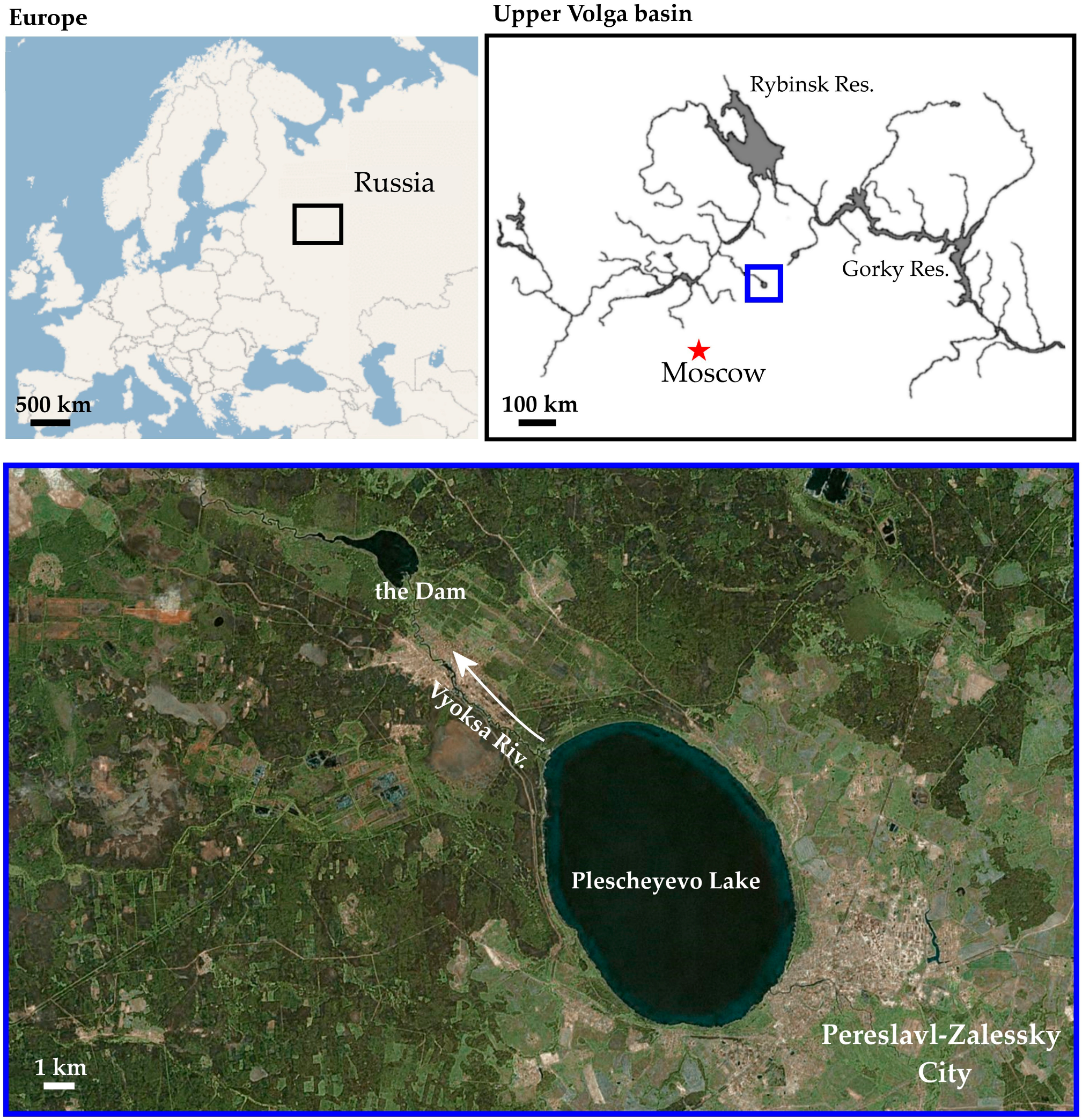
2.1. Sampling

Lake Plescheyevo (56.76° N; 38.78° E) is a water body in Central Russia (Figure 1) with a shoreline of ca. 27 km and area of 51.5 km². The lake has an oval shape, its littoral zone has a depth of up to 3 m and it occupies ca. 20% of the total area of the lake. The town of Pereslavl-Zalessky, with a population of about 40,000, is situated on the south shore of the lake [56]. The lake is connected with the Upper Volga by the relatively small Vyoksa River. However, the latter is impeded by a dam 5 km away from its source for regulation of the flood level; this dam causes considerable isolation of the lake and its fish population from the Volga basin. Lake Plescheyevo has extremely poor ichthyofauna—only 12 species of fish have been identified here by morphological methods [55].

Fish were sampled during the field seasons of 2014–2016 from May to October, by means of gill nets in the littoral zone, in the following three biotopes: in the area of Solomidino village (56.75535° N, 38.74237° E), near the Urev site (56.79983° N, 38.75352° E) and in the area of the Kukhmarka river mouth (56.79542° N, 38.78621° E). A total of 117 gill net catches were processed. Overall net exposure was 760 h. In addition, fish fry in the littoral zone were caught using the minnow seine. All catches were analyzed according to standard methods [57,58]. For molecular genetic analysis, a portion of the caudal fin blade or a piece of skin and muscle behind the dorsal fin was taken from each specimen and fixed in 95% ethanol cooled to −20 °C, while the voucher specimen was fixed in 4% formalin for subsequent morphological analysis. All vouchers are kept in the collection of the Ecology of Fishes of the Papanin Institute for Biology of Inland Waters of the Russian Academy of Sciences, Borok, Russia (see Supplementary Table S1).

2.2. From DNA Extraction to Phylogenetic Analysis

Sample preparation, total DNA isolation, PCR reactions and Sanger sequencing were performed according to a previously published protocol [52]. Primary analysis of the chromatograms, contig assemblage and sequence editing was made in the Sanger Reads Editor block of the uGENE ver. 46 package (Unipro, Novosibirsk, Russia) [59]. The original sequences were deposited with GenBank (National Center for Biotechnology Information, Bethesda MD, USA) under numbers KT989758-73 and KY228990. Previously obtained COI sequences for fish from this lake were included in the analysis, namely KT254047-49, KT254051, KT254053, KT254055. A sequence GQ328816 [60] of the Siberian sturgeon (Acipenser baerii) was used as an a-priori outgroup. For comparative purposes, for each taxon we took from the NCBI GenBank, by the ‘megablast’ query [61], several closest and several maximally distant (by criterion E-value with 100% Query Cover) sequences of the same taxon with a maximally wide geographic coverage. The sequences unambiguously belonging to the congener taxa were included in the analysis. As a result, we formed a set of 125 sequences for precise taxon identification and delimitation (see Supplementary Table S1). Ambiguous taxonomic marks (sp., cf., complex, clade) were removed from our analysis, because they are useless for accurate species delimitation. As a result, we had sequences from seven families of Actinopterygii. The taxonomy is represented according to the last edition of FishBase, ver. 02/2023 [62].

If not specially described below, all the calculations were made in “Microsoft R-Open and MKL” 64-bit ver. 3.5 (Microsoft Corp., Redmond, WA, USA; http://mran.microsoft.com/, accessed on 15 January 2023), Python 64-bit ver. 3.11 (Python Software Foundation, Dover, DE, USA; http://www.python.org/, accessed on 15 January 2023), or Java Development Kit 64-bit ver. 19 (Oracle Corp., Redwood Shores, CA, USA; http://jdk.java.net, accessed on 15 January 2023) with necessary packages installed. For this work, we principally used only public and non-commercial open-source software. Simple scripts in “R” for the delimitation is represented in Appendix A.

Sequence alignment was performed using the MAFFT ver. 7.5 [63], with “Translation Align” options, and the FFT-NS-I strategy. Phylogeny was reconstructed based on a whole set of “unlinked” data using [64] maximum likelihood (ML), Bayesian inference (BI) and maximum parsimony (MP).

ModelFinder ver. 1.6 [65] was used to search for the best model of nucleotide substitutions on the web portal of the Center for Integrative Bioinformatics (CIBIV, Vienna, Austria; http://www.iqtree.org, accessed on 17 January 2023) [66]. The substitution pattern was identified for each nucleotide position in the codon (1st—TIM3e + G4; 2nd—F81 + F + I; 3th—TN + F + G4), based on the minimum values of the Bayesian information criterion, BIC [67]. It should be noted that the parameters of the BIC model were almost identical to those determined on the basis of the corrected Akaike’s information criterion, AICc, which may indicate high agreement of the calculated models with the real best model [68].

For maximum likelihood (ML) analysis, we used the IQ-TREE ver. 2.2 algorithm [69]. As a branch support test, we used 10 k replicas of the UFboot2 bootstrap test [70]. Topology estimation for ML trees was based on 1 k replicates of SH-aLRT test [71], realized in the Building Phylogenetic Tree block of the uGENE. The ML tree constructed from the initial data was a realized (and not true) phylogenetic tree, and for such a case there is no unambiguous opinion about the correctness of using topological tests to check the monophyly of certain branches. However, in combination with a standard bootstrap, this procedure can be useful for assessing the group monophyly [72].

Maximum parsimony (MP) tree was achieved using a high-speed “New Technology” algorithm TNT ver. 1.5 [73]. As a branch support test, we used a standard bootstrap with 1 k replicas [74].

Reconstruction of the phylogeny using Bayesian inference (BI) was carried out using the BEAST2 ver. 2.7 software package [75] and the recommendations of [76]. Each analysis included six independent runs of MCMC, 50 M generations each, and selection of each 10 k tree. The effectiveness of MCMC on the convergence of the results of all independent runs with the estimated effective sample size (ESS) for all parameters above 200 was carried out with the Tracer ver. 1.7 program [77]. After combining the results of all MCMC runs through LogCombiner ver. 2.7 [78], a consensus tree was computed, based on the maximum confidence clade (MCC) using TreeAnnotator ver. 2.7 [78] with 25% burn-in.

2.3. Different Methods of mOTUs Delimitation

We performed a comparative analysis of almost all available and widely used methods of molecular operational taxonomic units, mOTUs [79] realized in different software packages.

Traditional identification of vouchers. Primary identification of our vouchers was based on morphological characters, and, then, sequences were compared to the reference sequences in two international databases: NCBI GenBank [30] and The Barcode of Life Data System [29]. A search of GenBank was conducted through the high speed HS-BLASTN [80] query. The exact identification was represented according to the NCBI Taxonomy Database [81]. Species identification in BOLD was performed through the ‘bold_identification’ script [82] with the demonstration of 10 best fits in automatic mode. Note that just the initial author’s identifications were used for the GenBank and BOLD sequences, without the possibility to check accurateness and correspondence to recent fish taxonomy.

Approach based on the population genetic theory. Our analysis included calculations of the K (the average pair distance between putative species-level clades) over Theta (estimation of the genetic diversity) rate, performed with the “KoT—K over Theta” ver. 1 package [31]. To prevent excessive splitting, we set up a stricter (>6) K/Theta threshold value, used for species delimitation with p < 0.01. It is known that the population genetic method, and, in particular “K over Theta”, depends excessively on nucleotide diversity, volume of studied material, population structure and even peculiarities in the migrations within the taxon [72]. Use of the standard value of K/Theta < 4 leads to identification as species of some clades which are apparently not species. We increased the threshold value to K/Theta < 6 as a way to resolve the problem of excessive “splitting” in the method [83].

The threshold-based delimitation methods. Analysis based on a direct calculation of the genetic divergence [4], keeping in mind the threshold value of 2.1%, was performed with the TaxonDNA/SpeciesIdentifier ver. 1.8 program [33]. The second approach [84], based on the “barcode gap” concept and formalized in the “Local Minima” function (locMin), was realized with the ‘spider’ package [85]. A simple script in “R” for the locMin calculation and the delimitation using this approach is represented in Appendix A. Our calculated threshold of 3.2% agreed well with the literature data [32] and was used for the “species gaps” findings in further automatic methods of the delimitation, as follow: ABGD, Automatic Barcode Gap Discovery [86] and ASAP, Assemble Species by Automatic Partitioning [87] through the ‘asapy’ and ‘abgdpy’ scripts of the iTaxoTools ver. 0.1 package [46], based on “simple” p-distances as the most preferable for barcoding purposes [88].

It is known that among the “barcoding gap” methods, a key moment is genetic threshold determination, which is based on some empirical observations. The level of 2.1–2.5% is most frequently used for fishes [89], but we need to note that this method is relatively effective for the COI locus only, with a great number of sequences deposited in GenBank. Using the SpeciesIdentifier, we needed to take into consideration that the threshold could be different in different genera, and even in families [90]. An automatic search for the “gaps” has some limitations, both in ABGD and ASAP, which could be partly resolved if the threshold is calculated separately using the locMin algorithm [91], although the latter tends to give thresholds that are too conservative for the discrimination of slightly different species.

Method of the Generalized Mixed Yule Coalescent (GMYC). If different variants of the GMYC realization led to similar delimitation results [35], we selected a “classical” scheme in the ‘splits’ package [92]. Bayesian implementation was performed with the ‘bgmyc’ package [93]. Our analysis followed an algorithm successively applied by us for invertebrates [94]. The cladogenesis threshold was determined to be p < 0.01 to prevent the possibility of redundant “splitting”. The scripts for “R” for the calculation of GMYC and bGMYC are represented in Appendix A. Note that a correct realization of ‘bgmyc’ is better performed in “R” ver. 3.x (The R Foundation for Statistical Computing, Vienna, Austria) while some bugs are possible in more recent versions.

GMYC has recently become one of the most frequently used delimitation methods, and just ‘splits’ realization is widely used in frames of the “traditional model” [34,92], because of its “just add water” approach. However, it is known that such delimitation results in excessive “splitting” [95]. Moreover, GMYC has a limitations in its objective representation of data and biological uncertainty of models [96]. Bayes realization in the ‘bgmyc’ package has a large set of adjusted parameters and works better with incomplete and strongly diverse datasets [93]. A strict criterion of p < 0.01 must be used to prevent false positive results [97].

Tree analysis based on the Poisson tree processes (PTP). Initial Python codes for realization of PTP and Bayesian implementation of PTP are published at their GitHub repositories: (b) PTP at https://github.com/zhangjiajie/PTP (accessed on 20 January 2023) and mPTP at https://github.com/Pas-Kapli/mptp (accessed on 20 January 2023). In all cases, we used the ML and kept the outgroup [27] as the input tree, and all other values were set up according to general recommendations for trees with a smaller (<50) number of taxa [36,37].

PTP is a powerful delimitation method, which has traditional (PTP) and Bayesian (bPTP) realizations [36], and also has the most powerful multi-rate version (mPTP) [37]. Note that mPTP works well just with mitochondrial genes demonstrating no incomplete lineage sorting and hybridization consequences.

Delimitation using the multispecies coalescent model. Our analysis was performed with the additional packages of BEAST2: “Species Tree And Classification Estimation, Yarely”— STACEY ver. 1.3 [38] and “SPEciEs DEliMitatiON”—SPEEDEMON ver. 1.1 [39]. All calculations were made in BEAST2 with the parameters were as in the phylogenetic analysis (see Section 2.2). Formation of the input XML files and their analysis and post-processing were performed according to the manufacturer recommendations.

The main advantage of delimitation using GMYC is that we did not need an a-priori species identification and an input tree. In SPEEDEMON (in contrast to STACEY), the Yule–skyline collapse model is used, with the speciation rate changing in time [39]. Two models are made for a multi-locus analysis, and they are also applicable to the single-locus delimitation [98]. However, we needed to take into consideration the point of view [99] that multi-species coalescences in reality delimit the population structure instead of real biological species, and we needed to be very critical in our interpretation of such delimitations.

Haplotype network analysis. Our analysis was performed with the HaplowebMaker/CoMa ver. 1 [40], and the initial code. Java-realization, available at https://github.com/eeg-ebe/HaplowebMaker (accessed on 20 January 2023), operated as a pipeline, allowing construction of the haplotype network so as to obtain the partition matrix summarizing the partitions inferred from each marker, transforming them to a conspecificity matrix and, finally, visualizing the results. The Median Joining algorithm [100] was used for the network construction, with the default values of all parameters.

The haplotype network analysis has an advantage over the tree analysis due to its taking into consideration, and visualizing, many alternative relationships between haplotypes and their groupings into larger structures. Such an analysis is very important for revealing the centers and means of organism dispersion, population and demographic models and the geographic limits of species distribution [101,102]. Selection of mOTUs based on networks in HaplowebMaker/CoMa, as with any other methods of phylogeographic analysis, is more acceptable for the determination of monophyletic clades and lineages than species identification and delimitation. The results of any phylogeographic reconstruction depend on the volume of studied material and adequate representation of the distribution range by samples. Moreover, cases of recent biological invasions make such an analysis more complicated [103]. Therefore, it is necessary to be very critical in using haplotype networks for species delimitation.

Approach to compare different delimitation methods. A qualitative comparison of alternative partitions was performed in the LIMES ver. 1.3 [104] and CoMa ver. 1 [40] programs. The algorithms of LIMES are analogous to those of CoMa, but the former provides the possibility to calculate several indices and to conduct a comparative analysis of different delimitation methods i.e., Ctax [105] and MatchRatio [106]. The conspecificity matrices integrating the results from 15 different methods of species delimitation was visualized in “R” package ‘heatmap3’ [107].

As in Box’s aphorism “all models wrong” [108], here, we followed a “caution” taxonomic strategy in the interpretation of genetic data [41], whereby “in most contexts it is better to fail to delimit species than it is to falsely delimit entities that do not represent actual evolutionary lineages”. The delimitations with a minimal number of taxa were preferable to us, while a higher number of mOTUS was interpreted as excessive splitting.

All original materials, namely DNA sequences, alignments, phylogenetic trees and images, used in this study are publicly available in the Supplementary Material and the Open Science Framework repository (https://osf.io/uyk5j/, accessed on 9 May 2023).

3. Results

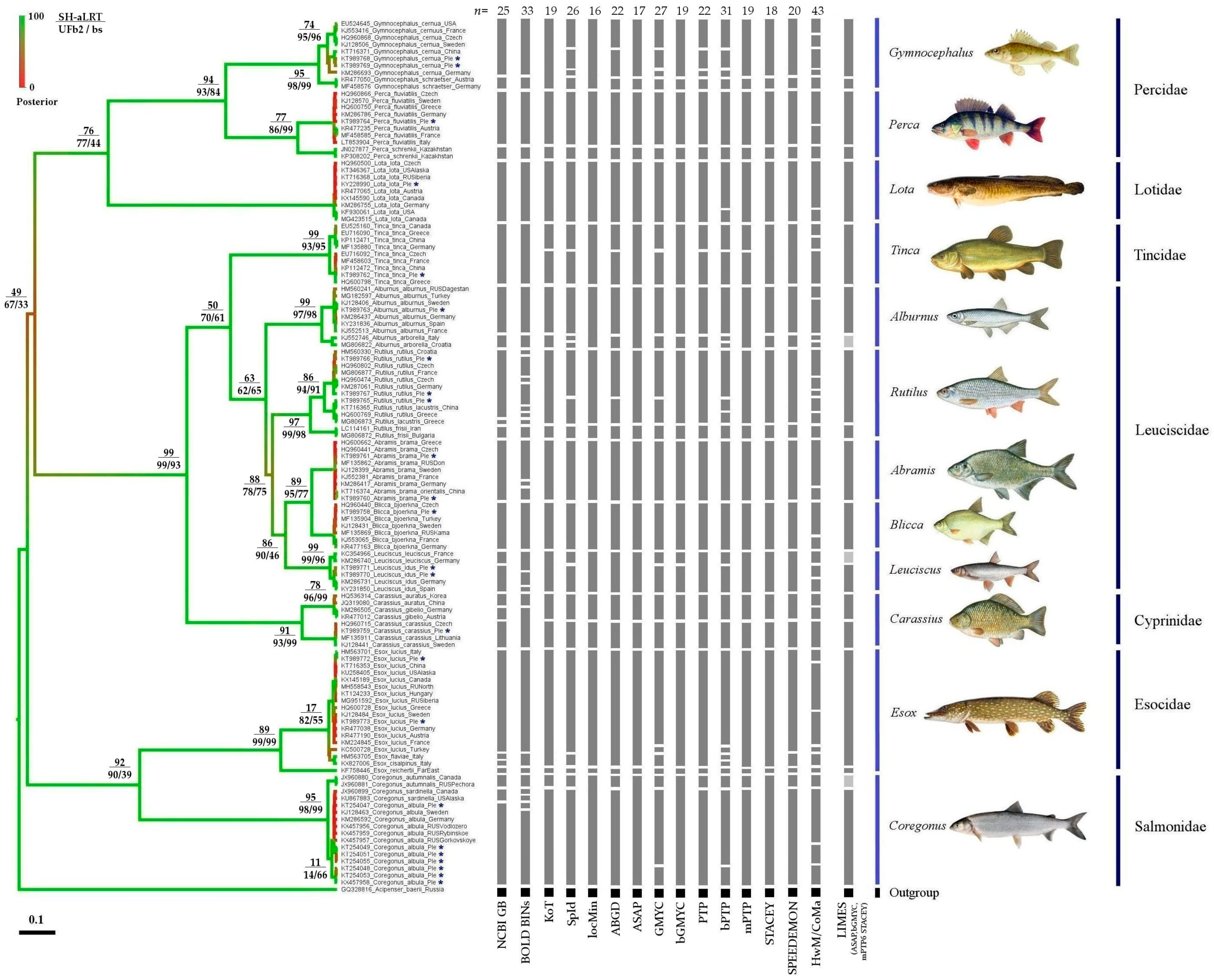
3.1. Phylogenetic Analysis

We performed genotyping of 186 fish specimens, 24 haplotypes (21 unique) having been deposited in GenBank. In total, 24 original sequences and 101 other sequences from the GenBank and BOLD were included in the analysis. A preliminary identification of each specimen, based on morphological characters, is represented in Supplementary Table S1.

Due to the full topological consistencies of the ML, BI and MP trees, we represented only the BI tree (Figure 2), with main branch support calculated by means of different methods.

Different approaches gave somewhat different support of deeper branches, although families and genera were, in general, well-supported by all methods. Lower values of the bootstrap could be explained by a low number of parsimony-informative sites in our dataset. A relatively high support was characteristic for the genera with the exclusion of all genera of Leuciscidae, but different species had different supports. Genetic clusters were fully consistent with the traditional morphospecies in Gymnocephalus, Perca, Lota, Abramis, Blicca. The Coregonus and Esox demonstrated some internal clusters, although their supports were low. It was possible to define supported intraspecies phylogenetic lineages within the species from the genera Carassius, Leusiscus, Tinca, Rutilus (Figure 2).

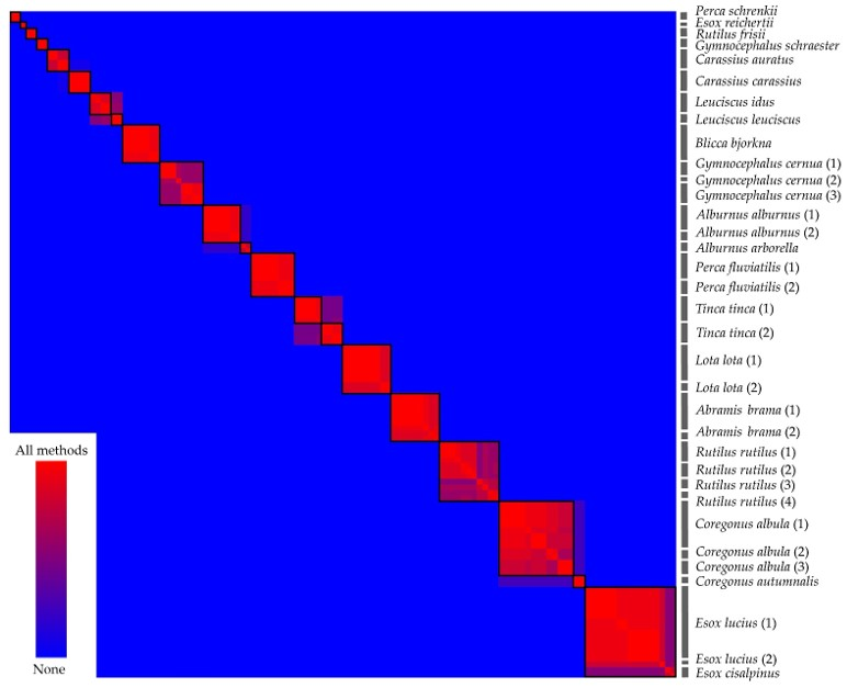
3.2. Comparison of Different Approaches to mOTU Delimitation

The results of 15 different methods of delimitation, based on the same genetic dataset, are represented in Figure 2 and Figure 3 and Supplementary Figures S1 and S2. Please take into consideration that the CoMa heatmap, represented in Figure 3, visualizes the conspecificity of delimitation methods rather than relationships between the taxa. All methods allowed unambiguous identification of all morphospecies inhabiting the lake, although some were represented by several OTUs. Different methods of the delimitation suggested different numbers of mOTUs (presumable biological species): from 16 (locMin) to 43 (HwM/CoMa) (Figure 2).

After comparison with our original sequences, we concluded that most sequences in Genbank and BOLD were correctly identified by their depositors, with the exception of three species of the genus Coregonus—C. albula, C. sardinella and C. autumnalis. Note that BOLD referred to one-third more taxa relative to the more conservative GenBank (33 vs. 25). KoT delimitation suggested a lower taxonomic diversity (only 19 mOTUs). In fact, these mOTUS were consistent with traditional morphospecies with the exception of the genera Leuciscus, where L. idus and L. leuciscus were not differentiated, and Tinca with T. tinca were represented by two phylogenetic lineages. The methods based on the “barcoding gap” gave differing results in that SpId and ABGD suggested many more mOTUs (26 and 22, respectively) than locMin and ASAP (17 mOTUs). In the last case, the mOTUs were consistent with traditional morphospecies, with the exception of the genus Coregonus (as above Figure 2). “Classical” GMYC excessively split the clades (27 mOTUs), while Bayes realization provided only 19 mOTUs. The same differences were observed for the Poisson tree processes, whereby the mPTP approach provided 19 and the bPTP approach provided 31. The former supported mainly the “traditional” morphospecies while the latter also supported a separation of some recently described taxa and some other independent phylogenetic lineages (see Section 4). Both variants on the coalescent-based analysis separated a similar number of mOTUs (18 and 20), the differences between them concerned the genera Esox and Coregonus (as above Figure 2). Finally, HaplowebMaker provided the maximum number of mOTUs — 43, which was an unacceptable splitting. Comparison of all 15 alternative taxonomies, based on the Ctax and MatchRatio criteria (

Table 1. Results of the comparison of 15 alternative delimitations. Values of Ctax are represented above the diagonal; MatchRatio (%) are below the diagonal. Bold type marks the values above 75%. Methods of species delimitation: GB—NCBI GenBank database; BN—“BINs”, Barcode Index Numbers, Barcode of Life Data Systems; KoT—“K over Theta” population genetics; SI—“TaxonDNA/SpeciesIdentifier” distance; LM—“local Minima” by ‘spider’; AB—“ABGD”, Automatic Barcode Gap Discovery; AS—“ASAP”, Assemble Species by Automatic Partitioning; YC—“GMYC”, mixed Yule-coalescent by ‘splits’; bYC—“bGMYC”, Bayesian Yule-coalescent by ‘bgmyc’; PT—“PTP”, Poisson Tree Processes model; bPT—“bPTP”, Bayesian Poisson Tree Processes; mPT—“mPTP”, multi-rate Poisson Tree Processes; STC—coalescence “STACEY”, Species Tree And Classification Estimation, Yarely; SPD—coalescence “SPEEDEMON”, SPEciEs DEliMitatiON; HwM—“Haploweb Maker”, haplotype webs and nets analysis.

	GB	BN	KoT	SI	LM	AB	AS	YC	bYC	PT	bPT	mPT	STC	SPD	HwM
GB		60	68	69	62	67	67	67	75	67	64	68	71	79	47
BN	52		47	46	42	47	45	41	47	47	44	47	48	55	42
KoT	50	35		72	83	86	79	69	80	86	60	89	84	85	40
SI	55	37	62		60	77	4	76	72	84	77	72	68	76	52
LM	44	29	74	43		71	94	58	83	71	50	83	88	79	36
AB	51	36	83	67	58		76	81	77	91	70	86	81	82	47
AS	52	36	67	47	91	62		62	89	76	53	89	94	84	38
YC	58	33	61	72	42	73	45		69	81	87	69	65	67	55
bYC	68	42	68	58	74	63	83	61		77	60	80	94	85	43
PT	51	36	88	75	63	86	67	73	68		70	86	81	82	47
bPT	50	25	48	70	34	57	38	79	48	60		60	57	63	64
mPT	50	35	84	62	74	78	83	57	68	83	48		84	85	40
STC	60	43	76	50	82	70	91	53	92	75	41	76		89	40
SPD	67	53	77	65	67	71	76	55	77	76	43	77	84		45
HwM	26	18	16	35	14	18	17	29	19	25	46	19	16	22

), allowed us to conclude that they adequately separated only the genera and most differentiated species.

We concluded that using a full set of these methods in a single study is redundant. We assumed that the effectiveness of each method correlated with the number of matches in each analysis, so bGMYC, mPTP, STACEY, KoT and ASAP provided the most comparable results (Figure 3), and the most synchronous results were obtained from bGMYC, STACEY, ASAP and mPTP (Table 1). We believe that these results are maximally realistic in the number of revealed mOTUs.

4. Discussion

In many cases, routine genetic species identification includes only a comparison of original sequences with some reference sequences in the international databases. It is necessary to take into consideration that the latter could be contaminated by DNA of other organisms [109] or represent initially incorrectly identified taxa [110]. Sometimes the barcoding results need to be specially “de-coded” [8]. The situation is also made more complicated by hybridization, whereby a specimen belongs to a certain morphospecies taxon, while sequences of its mitochondrial genes belong to a second species [111,112]. Finally, difficulties in using a “simple” comparison with references for species identification could be related to an unstable group taxonomy, personal preferences of previous authors and the aforementioned “taxonomic inflation” [24]. We recommend a comparison with the NCBI GenBank and BOLD reference barcodes as the first step in sequence identification only, instead of being a good method for species delimitation. For the latter, a combination of several advanced methods based on different approaches is necessary.

Above, we describe a particular situation when the results of different delimitation methods contradicted each other. Such differences could be partly explained by the known shortcomings of each method (see Section 2.3 above) but the rate of such differences probably varies between different taxa due to differences in their genetic patterns.

Different methods could suggest a very different number of mOTUs in a genetic dataset. In our case, as usual, a better correspondence of delimitation by different algorithms was observed in well-studied groups with a relatively simple taxonomic structure. A mismatch of one or more methods in a particular group is a signal for taxonomists to pay closer attention to it [20]. In our dataset, the mOTUs in the genera Gymnocephalus, Perca, Lota, Alburnus, Abramis, Blicca almost each time corresponded well to the traditional morphospecies (Supplementary Table S1). Separation of several mOTUs within some other taxa could be explained by their disjunctive distribution ranges resulting from dispersion from isolated glacial refugia during the Pleistocene age, as in the case of Tinca tinca [113]. The genetic pattern of the Carassius auratus complex is probably related to a distribution range disjunction and a subsequent anthropogenic introduction of the Far Eastern lineage to Europe [114].

At the same time, some conclusions on the species delimitation do not depend on the approach. Remarkably, most methods did not support separation of such traditional fish morphospecies as Leuciscus leuciscus and L. idus (see initial identifications of the sequences from GenBank and BOLD in our tree, Figure 2). Most methods did not support a separation of several taxa within Esox lucius and Rutilus rutilus, in contrast to the opinions of some recent investigators [115,116]. Finally, within the genus Coregonus we observed low genetic differentiation [117] between traditionally separated [118] species, such as European (C. albula) and Siberian (C. sardinella) vendace. Only the Arctic cisco (C. autumnalis) represented a separate mOTU (Figure 2). Most delimitations supported the opinion [119] on the inexpediency of accepting C. albula and C. sardinella as separate species.

We demonstrated again that different mathematical methods suggest separation of different mOTU numbers. It should be noted that results of any phylogeographic reconstructions depend on the volume of studied material and adequate representation of all the distribution range by samples, moreover, cases of recent biological invasions make such analysis more complicated [120].

To date, about 30 different species concepts have been proposed, based on different criteria, and some of them apparently contradict each other [121]. In general, species and mOTUs are different matters [122], although in many publications (especially in cases of cryptic species) they are accepted as identical [123], and such identity at least requires a special study [124]. According to the “phylogenetic species” concept, any population of a non-hybrid origin could be regarded as a species [125]. We think that a more adequate solution for species delimitation is to return to the “polymorphic” or “polytypic” species [126,127,128]. These two concepts are similar in species interpretation. The polymorphic species [127] unites several allopatric and sympatric population groups, while the polytypic species is a complex unit subdivided into subspecies and geographic races [128]. In any case, the animal groups are regarded as morphs or subspecies in cases of the absence of reproductive isolation, and as independent species in cases of its presence. Species polymorphism is not doubted by any investigators [129], and phylogenetic lineages, morphs and races are well known in different animals [94,130,131,132]. There are no problems in using such concepts for interpretation of genetic data, with phylogenetic lineages providing the species polymorphism instead of being separate taxa in the understanding of the International Code of Zoological Nomenclature [133].

Acceptance of the local populations as separate species is a way to simplify legislative implementation (including any red lists) and fundraising for their protection [22]. Based on such approach, we can regard some phylogenetic lines of vendace from Plescheyevo Lake as a separate species (it does not contradict the genetic data [134]) and based on some delimitation methods giving a larger number of mOUTs but we believe that this is not a scientific approach [135]. In our case, just the vendace population from Plescheyevo Lake is included in the Red Book of Russian Federation [53], while this species is not protected in all other territories of the country.

We need to remember that DNA barcoding is not a fully universal method, and, in some cases, it is not able to differentiate “good” species well supported by nuclear phylogenies, due to complex reasons not discussed in our paper, see [136]. Only a combination of different methods (study of mitochondrial, nuclear genes and morphology) could lead to adequate understanding of the biodiversity in different water bodies.

5. Conclusions

In this study we report on the DNA barcoding of all mass fish species in Plescheyevo Lake and we used these barcodes, plus those from international databases, to compare 15 different methods of species delimitation. Based on the fits between different methods, we conclude that the effectiveness of different methods strongly differ, but bGMYC, STACEY, ASAP with locMin and mPTP provided the most synchronous results. Moreover, it is necessary to take into consideration the opportunities and limitations of each method in each particular case. A-priori reasons to use a particular method are not well-formulated to date, and for an accurate and comprehensive estimation of biodiversity, we need to use a combination of several methods based on different approaches. High genetic diversity results in the existence of several mOTUs and phylogenetic lineages within many species and demonstrates the usefulness of the “polymorphic species” concept, which does not underestimate species richness and does not prevent the rational use and protection of biodiversity.

References

1. UNCED. AGENDA 21: The Earth Summit Strategy to Save Our Planet. Available online: https://sustainabledevelopment.un.org/outcomedocuments/agenda21 (accessed on 7 July 2022).
2. Templeton, A.R. Using phylogeographic analyses of gene trees to test species status and processes. Mol. Ecol. 2001, 10, 779–791. [Google Scholar] [CrossRef] [PubMed]
3. van Klink, R.; Bowler, D.E.; Gongalsky, K.B.; Swengel, A.B.; Gentile, A.; Chase, J.M. Meta-analysis reveals declines in terrestrial but increases in freshwater insect abundances. Science 2020, 368, 417–420. [Google Scholar] [CrossRef] [PubMed]
4. Hebert, P.D.N.; Cywinska, A.; Ball, S.L.; de Waard, J.R. Biological identifications through DNA barcodes. Proc. R. Soc. Lond. B Biol. Sci. 2003, 270, 313–321. [Google Scholar] [CrossRef] [PubMed]
5. Trewick, S.A. DNA Barcoding is not enough: Mismatch of taxonomy and genealogy in New Zealand grasshoppers (Orthoptera: Acrididae). Cladistics 2008, 24, 240–254. [Google Scholar] [CrossRef]
6. Ebach, M.C.; de Carvalho, M.R. Anti-intellectualism in the DNA barcoding enterprise. Zoologia 2010, 27, 165–178. [Google Scholar] [CrossRef]
7. Taylor, H.R.; Harris, W.E. An emergent science on the brink of irrelevance: A review of the past 8 years of DNA barcoding. Mol. Ecol. Resour. 2012, 12, 377–388. [Google Scholar] [CrossRef]
8. Garibian, P.G.; Neretina, A.N.; Taylor, D.J.; Kotov, A.A. Partial revision of the neustonic genus Scapholeberis Schoedler, 1858 (Crustacea: Cladocera): Decoding of the barcoding results. PeerJ 2020, 8, e10410. [Google Scholar] [CrossRef]
9. Zamani, A.; Fric, Z.F.; Gante, H.F.; Hopkins, T.; Orfinger, A.B.; Scherz, M.D.; Bartonova, A.S.; Pos, D.D. DNA barcodes on their own are not enough to describe a species. Syst. Entomol. 2022, 47, 385–389. [Google Scholar] [CrossRef]
10. Will, K.W.; Rubinoff, D. Myth of the molecule: DNA barcodes for species cannot replace morphology for identification and classification. Cladistics 2004, 20, 47–55. [Google Scholar] [CrossRef]
11. Hellmuth, M. Biologically feasible gene trees, reconciliation maps and informative triples. Algorithms Mol. Biol. 2017, 12, 23. [Google Scholar] [CrossRef]
12. Andujar, C.; Arribas, P.; Yu, D.W.; Vogler, A.P.; Emerson, B.C. Why the COI barcode should be the community DNA metabarcode for the metazoa. Mol. Ecol. 2018, 27, 3968–3975. [Google Scholar] [CrossRef]
13. Rubinoff, D.; Cameron, S.; Will, K. Are plant DNA barcodes a search for the Holy Grail? Trends Ecol. Evol. 2006, 21, 1–2. [Google Scholar] [CrossRef]
14. Vijayan, K.; Tsou, C.-H. DNA barcoding in plants: Taxonomy in a new perspective. Curr. Sci. 2010, 99, 1530–1541. [Google Scholar]
15. Lebonah, D.E.; Dileep, A.; Chandrasekhar, K.; Sreevani, S.; Sreedevi, B.; Pramoda Kumari, J. DNA barcoding on Bacteria: A review. Adv. Biol. 2014, 2014, 541787. [Google Scholar] [CrossRef]
16. Xu, J. Fungal DNA barcoding. Genome 2016, 59, 913–932. [Google Scholar] [CrossRef]
17. Rubinoff, D.; Cameron, S.; Will, K. A genomic perspective on the shortcomings of mitochondrial DNA for “barcoding” identification. J. Hered. 2006, 97, 581–594. [Google Scholar] [CrossRef]
18. Raupach, M.J.; Amann, R.; Wheeler, Q.D.; Roos, C. The application of “-omics” technologies for the classification and identification of animals. Org. Divers. Evol. 2016, 16, 1–12. [Google Scholar] [CrossRef]
19. Coissac, E.; Hollingsworth, P.M.; Lavergne, S.; Taberlet, P. From barcodes to genomes: Extending the concept of DNA barcoding. Mol. Ecol. 2016, 25, 1423–1428. [Google Scholar] [CrossRef]
20. Guo, B.; Kong, L. Comparing the efficiency of single-locus species delimitation methods within Trochoidea (Gastropoda: Vetigastropoda). Genes 2022, 13, 2273. [Google Scholar] [CrossRef]
21. Isaac, N.J.B.; Mallet, J.; Mace, G.M. Taxonomic inflation: Its influence on macroecology and conservation. Trends Ecol. Evol. 2004, 19, 464–469. [Google Scholar] [CrossRef]
22. Cotterill, F.P.D.; Taylor, P.J.; Gippoliti, S.; Bishop, J.M.; Groves, C.P. Why one century of phenetics is enough: Response to “Are there really twice as many bovid species as we thought?”. Syst. Biol. 2014, 63, 819–832. [Google Scholar] [CrossRef] [PubMed]
23. Primack, R.B. Essentials of Conservation Biology, 6th ed.; Sinauer Associates: Sunderland, MA, USA, 2014; ISBN 978-1605352893. [Google Scholar]
24. Zachos, F.E. Taxonomic inflation, the Phylogenetic Species Concept and lineages in the Tree of Life—A cautionary comment on species splitting. J. Zool. Syst. Evol. Res. 2015, 53, 180–184. [Google Scholar] [CrossRef]
25. Jaric, I.; Heger, T.; Castro Monzon, F.; Jeschke, J.M.; Kowarik, I.; McConkey, K.R.; Pysek, P.; Sagouis, A.; Essl, F. Crypticity in biological invasions. Trends Ecol. Evol. 2019, 34, 291–302. [Google Scholar] [CrossRef] [PubMed]
26. Kotov, A.A.; Karabanov, D.P.; Van Damme, K. Non-indigenous cladocera (Crustacea: Branchiopoda): From a few notorious cases to a potential global faunal mixing in aquatic ecosystems. Water 2022, 14, 2806. [Google Scholar] [CrossRef]
27. Vitecek, S.; Kucinic, M.; Previsic, A.; Zivic, I.; Stojanovic, K.; Keresztes, L.; Balint, M.; Hoppeler, F.; Waringer, J.; Graf, W.; et al. Integrative taxonomy by molecular species delimitation: Multi-locus data corroborate a new species of Balkan Drusinae micro-endemics. BMC Evol. Biol. 2017, 17, 129. [Google Scholar] [CrossRef]
28. Solovyeva, E.N.; Dunayev, E.A.; Nazarov, R.A.; Bondarenko, D.A.; Poyarkov, N.A. COI-barcoding and species delimitation assessment of toad-headed Agamas of the genus Phrynocephalus (Agamidae, Squamata) reveal unrecognized diversity in Central Eurasia. Diversity 2023, 15, 149. [Google Scholar] [CrossRef]
29. Ratnasingham, S.; Hebert, P.D.N. BOLD: The Barcode of Life Data System (http://www.barcodinglife.org). Mol. Ecol. Notes 2007, 7, 355–364. [Google Scholar] [CrossRef]
30. Sayers, E.W.; Cavanaugh, M.; Clark, K.; Ostell, J.; Pruitt, K.D.; Karsch-Mizrachi, I. GenBank. Nucleic Acids Res. 2019, 47, D94–D99. [Google Scholar] [CrossRef]
31. Spori, Y.; Stoch, F.; Dellicour, S.; Birky, C.W.; Flot, J.-F. KoT: An automatic implementation of the K/θ method for species delimitation. bioRxiv 2021. [Google Scholar] [CrossRef]
32. Hebert, P.D.N.; Stoeckle, M.Y.; Zemlak, T.S.; Francis, C.M. Identification of Birds through DNA Barcodes. PLoS Biol. 2004, 2, e312. [Google Scholar] [CrossRef]
33. Meier, R.; Shiyang, K.; Vaidya, G.; Ng, P.K.L. DNA barcoding and taxonomy in Diptera: A tale of high intraspecific variability and low identification success. Syst. Biol. 2006, 55, 715–728. [Google Scholar] [CrossRef]
34. Pons, J.; Barraclough, T.G.; Gomez-Zurita, J.; Cardoso, A.; Duran, D.P.; Hazell, S.; Kamoun, S.; Sumlin, W.D.; Vogler, A.P. Sequence-based species delimitation for the DNA taxonomy of undescribed insects. Syst. Biol. 2006, 55, 595–609. [Google Scholar] [CrossRef]
35. Da Silva, R.; Peloso, P.L.V.; Sturaro, M.J.; Veneza, I.; Sampaio, I.; Schneider, H.; Gomes, G. Comparative analyses of species delimitation methods with molecular data in Snappers (Perciformes: Lutjaninae). Mitochondrial DNA Part A 2018, 29, 1108–1114. [Google Scholar] [CrossRef]
36. Zhang, J.; Kapli, P.; Pavlidis, P.; Stamatakis, A. A general species delimitation method with applications to phylogenetic placements. Bioinformatics 2013, 29, 2869–2876. [Google Scholar] [CrossRef]
37. Kapli, P.; Lutteropp, S.; Zhang, J.; Kobert, K.; Pavlidis, P.; Stamatakis, A.; Flouri, T. Multi-rate Poisson tree processes for single-locus species delimitation under maximum likelihood and Markov chain Monte Carlo. Bioinformatics 2017, 33, 1630–1638. [Google Scholar] [CrossRef]
38. Jones, G. Algorithmic improvements to species delimitation and phylogeny estimation under the multispecies coalescent. J. Math. Biol. 2017, 74, 447–467. [Google Scholar] [CrossRef]
39. Douglas, J.; Bouckaert, R. Quantitatively defining species boundaries with more efficiency and more biological realism. Commun. Biol. 2022, 5, 755. [Google Scholar] [CrossRef]
40. Spori, Y.; Flot, J.-F. HaplowebMaker and CoMa: Two web tools to delimit species using haplowebs and conspecificity matrices. Methods Ecol. Evol. 2020, 11, 1434–1438. [Google Scholar] [CrossRef]
41. Carstens, B.C.; Pelletier, T.A.; Reid, N.M.; Satler, J.D. How to fail at species delimitation. Mol. Ecol. 2013, 22, 4369–4383. [Google Scholar] [CrossRef]
42. de Carvalho, M.R.; Bockmann, F.A.; Amorim, D.S.; Brandão, C.R.F.; de Vivo, M.; de Figueiredo, J.L.; Britski, H.A.; de Pinna, M.C.C.; Menezes, N.A.; Marques, F.P.L.; et al. Taxonomic impediment or impediment to taxonomy? A commentary on systematics and the cybertaxonomic-automation paradigm. Evol. Biol. 2007, 34, 140–143. [Google Scholar] [CrossRef]
43. Kotov, A.A.; Gololobova, M.A. Traditional taxonomy: Quo vadis? Integr. Zool. 2016, 11, 500–505. [Google Scholar] [CrossRef] [PubMed]
44. Dellicour, S.; Flot, J.-F. The hitchhiker’s guide to single-locus species delimitation. Mol. Ecol. Resour. 2018, 18, 1234–1246. [Google Scholar] [CrossRef] [PubMed]
45. Luo, A.; Ho, S.Y.W. The molecular clock and evolutionary timescales. Biochem. Soc. Trans. 2018, 46, 1183–1190. [Google Scholar] [CrossRef] [PubMed]
46. Vences, M.; Miralles, A.; Brouillet, S.; Ducasse, J.; Fedosov, A.; Kharchev, V.; Kostdinov, I.; Kumari, S.; Patmanidis, S.; Scherz, M.D.; et al. iTaxoTools 0.1: Kickstarting a specimen-based software toolkit for taxonomists. Megataxa 2021, 6, 77–92. [Google Scholar] [CrossRef]
47. Machado, V.N.; Collins, R.A.; Ota, R.P.; Andrade, M.C.; Farias, I.P.; Hrbek, T. One thousand DNA barcodes of piranhas and pacus reveal geographic structure and unrecognised diversity in the Amazon. Sci. Rep. 2018, 8, 8387. [Google Scholar] [CrossRef]
48. Hebert, P.D.N.; deWaard, J.R.; Landry, J.-F. DNA barcodes for 1/1000 of the animal kingdom. Biol. Lett. 2010, 6, 359–362. [Google Scholar] [CrossRef]
49. Valdez-Moreno, M.; Ivanova, N.V.; Elias-Gutierrez, M.; Contreras-Balderas, S.; Hebert, P.D.N. Probing diversity in freshwater fishes from Mexico and Guatemala with DNA barcodes. J. Fish Biol. 2009, 74, 377–402. [Google Scholar] [CrossRef]
50. Pereira, L.H.G.; Hanner, R.; Foresti, F.; Oliveira, C. Can DNA barcoding accurately discriminate megadiverse Neotropical freshwater fish fauna? BMC Genet. 2013, 14, 20. [Google Scholar] [CrossRef]
51. Turanov, S.V.; Kartavtsev, Y.P. A complement to DNA barcoding reference library for identification of fish from the Northeast Pacific. Genome 2021, 64, 927–936. [Google Scholar] [CrossRef]
52. Karabanov, D.P.; Bekker, E.I.; Pavlov, D.D.; Borovikova, E.A.; Kodukhova, Y.V.; Kotov, A.A. New sets of primers for DNA identification of non-indigenous fish species in the Volga-Kama basin (European Russia). Water 2022, 14, e437. [Google Scholar] [CrossRef]
53. Pavlov, D.S. (Ed.) Red Book of the Russian Federation, 2nd ed.; Volume “Animals”; FGBU “VNII Ecologiya”: Moscow, Russia, 2021; ISBN 978-5-6047425-0-1. [Google Scholar]
54. Kodukhova, Y.V.; Karabanov, D.P. Morphological changes in the population of roach (Rutilus rutilus, Cyprinidae) in lake Pleshcheevo as a result of the introduction of the mollusk, Dreissena polymorpha (Bivalvia). Zool. Zhurnal 2017, 96, 1069–1077. [Google Scholar] [CrossRef]
55. Smirnov, A.K.; Pavlov, D.D.; Kodukhova, Y.V.; Karabanov, D.P. Impact of Zebra mussel Dreissena polymorpha pallas 1771 (Bivalvia) appearance on fish populations in Lake Pleshcheevo, European Russia. Zool. Zhurnal 2020, 99, 1363–1374. [Google Scholar] [CrossRef]
56. Rosstat. Population Census: Official statistics. Available online: https://eng.rosstat.gov.ru/folder/76215 (accessed on 24 February 2023).
57. Pravdin, I.F. Guide for the Study of Fish; Pishchevaya Promyshlennost: Moscow, Russia, 1966. [Google Scholar]
58. Kottelat, M.; Freyhof, J. Handbook of European Freshwater Fishes; Publications Kottelat: Cornol, Switzerland, 2007; ISBN 2839902982. [Google Scholar]
59. Okonechnikov, K.; Golosova, O.; Fursov, M. Unipro UGENE: A unified bioinformatics toolkit. Bioinformatics 2012, 28, 1166–1167. [Google Scholar] [CrossRef]
60. Birstein, V.J.; DeSalle, R.; Doukakis, P.; Hanner, R.; Ruban, G.I.; Wong, E. Testing taxonomic boundaries and the limit of DNA barcoding in the Siberian sturgeon, Acipenser baerii. Mitochondrial DNA 2009, 20, 110–118. [Google Scholar] [CrossRef]
61. Morgulis, A.; Coulouris, G.; Raytselis, Y.; Madden, T.L.; Agarwala, R.; Schaffer, A.A. Database indexing for production MegaBLAST searches. Bioinformatics 2008, 24, 1757–1764. [Google Scholar] [CrossRef]
62. Froese, R.; Pauly, D. (Eds.) FishBase. World Wide Web Electronic Publication, Version 02/2023. Available online: www.fishbase.org (accessed on 23 February 2023).
63. Katoh, K.; Standley, D.M. MAFFT multiple sequence alignment software version 7: Improvements in performance and usability. Mol. Biol. Evol. 2013, 30, 772–780. [Google Scholar] [CrossRef]
64. Yang, Z.; Rannala, B. Molecular phylogenetics: Principles and practice. Nat. Rev. Genet. 2012, 13, 303–314. [Google Scholar] [CrossRef]
65. Kalyaanamoorthy, S.; Minh, B.Q.; Wong, T.K.F.; von Haeseler, A.; Jermiin, L.S. ModelFinder: Fast model selection for accurate phylogenetic estimates. Nat. Methods 2017, 14, 587–589. [Google Scholar] [CrossRef]
66. Trifinopoulos, J.; Nguyen, L.-T.; von Haeseler, A.; Minh, B.Q. W-IQ-TREE: A fast online phylogenetic tool for maximum likelihood analysis. Nucleic Acids Res. 2016, 44, W232–W235. [Google Scholar] [CrossRef]
67. Schwarz, G. Estimating the dimension of a model. Ann. Stat. 1978, 6, 461–464. [Google Scholar] [CrossRef]
68. Posada, D.; Buckley, T.R. Model selection and model averaging in phylogenetics: Advantages of Akaike information criterion and Bayesian approaches over likelihood ratio tests. Syst. Biol. 2004, 53, 793–808. [Google Scholar] [CrossRef] [PubMed]
69. Minh, B.Q.; Schmidt, H.A.; Chernomor, O.; Schrempf, D.; Woodhams, M.D.; von Haeseler, A.; Lanfear, R. IQ-TREE 2: New models and efficient methods for phylogenetic inference in the genomic era. Mol. Biol. Evol. 2020, 37, 1530–1534. [Google Scholar] [CrossRef] [PubMed]
70. Hoang, D.T.; Chernomor, O.; von Haeseler, A.; Minh, B.Q.; Le Vinh, S. UFBoot2: Improving the ultrafast bootstrap approximation. Mol. Biol. Evol. 2018, 35, 518–522. [Google Scholar] [CrossRef] [PubMed]
71. Shimodaira, H. An approximately unbiased test of phylogenetic tree selection. Syst. Biol. 2002, 51, 492–508. [Google Scholar] [CrossRef] [PubMed]
72. Nei, M.; Kumar, S. Molecular Evolution and Phylogenetics; Oxford University Press: New York, NY, USA, 2000; ISBN 0195135857. [Google Scholar]
73. Goloboff, P.A.; Catalano, S.A. TNT version 1.5, including a full implementation of phylogenetic morphometrics. Cladistics 2016, 32, 221–238. [Google Scholar] [CrossRef]
74. Felsenstein, J. Confidence limits on phylogenies: An approach using the bootstrap. Evolution 1985, 39, 783–791. [Google Scholar] [CrossRef]
75. Bouckaert, R.; Vaughan, T.G.; Barido-Sottani, J.; Duchene, S.; Fourment, M.; Gavryushkina, A.; Heled, J.; Jones, G.; Kuhnert, D.; de Maio, N.; et al. BEAST 2.5: An advanced software platform for Bayesian evolutionary analysis. PLoS Comput. Biol. 2019, 15, e1006650. [Google Scholar] [CrossRef]
76. Barido-Sottani, J.; Boskova, V.; Du Plessis, L.; Kuhnert, D.; Magnus, C.; Mitov, V.; Muller, N.F.; PecErska, J.; Rasmussen, D.A.; Zhang, C.; et al. Taming the BEAST—A community teaching material resource for BEAST2. Syst. Biol. 2018, 67, 170–174. [Google Scholar] [CrossRef]
77. Rambaut, A.; Drummond, A.J.; Xie, D.; Baele, G.; Suchard, M.A. Posterior summarization in Bayesian phylogenetics using Tracer 1.7. Syst. Biol. 2018, 67, 901–904. [Google Scholar] [CrossRef]
78. Drummond, A.J.; Bouckaert, R.R. Bayesian Evolutionary Analysis with BEAST2; Cambridge University Press: Cambridge, UK, 2015; ISBN 978-1-107-01965-2. [Google Scholar]
79. Floyd, R.; Abebe, E.; Papert, A.; Blaxter, M. Molecular barcodes for soil nematode identification. Mol. Ecol. 2002, 11, 839–850. [Google Scholar] [CrossRef]
80. Chen, Y.; Ye, W.; Zhang, Y.; Xu, Y. High speed BLASTN: An accelerated MegaBLAST search tool. Nucleic Acids Res. 2015, 43, 7762–7768. [Google Scholar] [CrossRef]
81. Schoch, C.L.; Ciufo, S.; Domrachev, M.; Hotton, C.L.; Kannan, S.; Khovanskaya, R.; Leipe, D.; Mcveigh, R.; O’Neill, K.; Robbertse, B.; et al. NCBI Taxonomy: A comprehensive update on curation, resources and tools. Database 2020, 2020, baaa062. [Google Scholar] [CrossRef]
82. Yang, C.; Zheng, Y.; Tan, S.; Meng, G.; Rao, W.; Yang, C.; Bourne, D.G.; O’Brien, P.A.; Xu, J.; Liao, S.; et al. Efficient COI barcoding using high throughput single-end 400 bp sequencing. BMC Genom. 2020, 21, 862. [Google Scholar] [CrossRef]
83. Birky, C.W. Species detection and identification in sexual organisms using population genetic theory and DNA sequences. PLoS ONE 2013, 8, e52544. [Google Scholar] [CrossRef]
84. Rangel-Medrano, J.D.; Ortega-Lara, A.; Marquez, E.J. Ancient genetic divergence in bumblebee catfish of the genus Pseudopimelodus (Pseudopimelodidae: Siluriformes) from northwestern South America. PeerJ 2020, 8, e9028. [Google Scholar] [CrossRef]
85. Brown, S.D.J.; Collins, R.A.; Boyer, S.; Lefort, M.-C.; Malumbres-Olarte, J.; Vink, C.J.; Cruickshank, R.H. Spider: An R package for the analysis of species identity and evolution, with particular reference to DNA barcoding. Mol. Ecol. Resour. 2012, 12, 562–565. [Google Scholar] [CrossRef]
86. Puillandre, N.; Lambert, A.; Brouillet, S.; Achaz, G. ABGD, Automatic Barcode Gap Discovery for primary species delimitation. Mol. Ecol. 2012, 21, 1864–1877. [Google Scholar] [CrossRef]
87. Puillandre, N.; Brouillet, S.; Achaz, G. ASAP: Assemble species by automatic partitioning. Mol. Ecol. Resour. 2021, 21, 609–620. [Google Scholar] [CrossRef]
88. Collins, R.A.; Boykin, L.M.; Cruickshank, R.H.; Armstrong, K.F. Barcoding’s next top model: An evaluation of nucleotide substitution models for specimen identification. Methods Ecol. Evol. 2012, 3, 457–465. [Google Scholar] [CrossRef]
89. Ward, R.D. DNA barcode divergence among species and genera of birds and fishes. Mol. Ecol. Resour. 2009, 9, 1077–1085. [Google Scholar] [CrossRef]
90. Kartavtsev, Y.P. Sequence divergence at mitochondrial genes in animals: Applicability of DNA data in genetics of speciation and molecular phylogenetics. Mar. Genom. 2011, 4, 71–81. [Google Scholar] [CrossRef] [PubMed]
91. Ota, R.P.; Machado, V.N.; Andrade, M.C.; Collins, R.A.; Farias, I.P.; Hrbek, T. Integrative taxonomy reveals a new species of pacu (Characiformes: Serrasalmidae: Myloplus) from the Brazilian Amazon. Neotrop. Ichthyol. 2020, 18, e190112. [Google Scholar] [CrossRef]
92. Fujisawa, T.; Barraclough, T.G. Delimiting species using single-locus data and the Generalized Mixed Yule Coalescent approach: A revised method and evaluation on simulated data sets. Syst. Biol. 2013, 62, 707–724. [Google Scholar] [CrossRef] [PubMed]
93. Reid, N.M.; Carstens, B.C. Phylogenetic estimation error can decrease the accuracy of species delimitation: A Bayesian implementation of the general mixed Yule-coalescent model. BMC Evol. Biol. 2012, 12, 196. [Google Scholar] [CrossRef]
94. Kotov, A.A.; Garibian, P.G.; Bekker, E.I.; Taylor, D.J.; Karabanov, D.P. A new species group from the Daphnia curvirostris species complex (Cladocera: Anomopoda) from the eastern Palaearctic: Taxonomy, phylogeny and phylogeography. Zool. J. Linn. Soc. 2021, 191, 772–822. [Google Scholar] [CrossRef]
95. Talavera, G.; Dinca, V.; Vila, R. Factors affecting species delimitations with the GMYC model: Insights from a butterfly survey. Methods Ecol. Evol. 2013, 4, 1101–1110. [Google Scholar] [CrossRef]
96. Lohse, K. Can mtDNA barcodes be used to delimit species? A response to Pons et al. (2006). Syst. Biol. 2009, 58, 439–442; Discussion 442–444. [Google Scholar] [CrossRef]
97. Neretina, A.N.; Karabanov, D.P.; Sacherova, V.; Kotov, A.A. Unexpected mitochondrial lineage diversity within the genus Alonella Sars, 1862 (Crustacea: Cladocera) across the Northern Hemisphere. PeerJ 2021, 9, e10804. [Google Scholar] [CrossRef]
98. Xu, R.; Lu, Y.; Tang, Y.; Chen, Z.; Xu, C.; Zhang, X.; Zheng, X. DNA barcoding reveals high hidden species diversity of Chinese waters in the Cephalopoda. Front. Mar. Sci. 2022, 9, 830381. [Google Scholar] [CrossRef]
99. Sukumaran, J.; Knowles, L.L. Multispecies coalescent delimits structure, not species. Proc. Natl. Acad. Sci. USA 2017, 114, 1607–1612. [Google Scholar] [CrossRef]
100. Bandelt, H.J.; Forster, P.; Rohl, A. Median-joining networks for inferring intraspecific phylogenies. Mol. Biol. Evol. 1999, 16, 37–48. [Google Scholar] [CrossRef]
101. Karabanov, D.P.; Kodukhova, Y.V.; Pashkov, A.N.; Reshetnikov, A.N.; Makhrov, A.A. “Journey to the West”: Three phylogenetic lineages contributed to the invasion of Stone Moroko, Pseudorasbora parva (Actinopterygii: Cyprinidae). Russ. J. Biol. Invasions 2021, 12, 67–78. [Google Scholar] [CrossRef]
102. Gu, Q.; Wang, S.; Zhong, H.; Yuan, H.; Yang, J.; Yang, C.; Huang, X.; Xu, X.; Wang, Y.; Wei, Z.; et al. Phylogeographic relationships and the evolutionary history of the Carassius auratus complex with a newly born homodiploid raw fish (2nNCRC). BMC Genom. 2022, 23, 242. [Google Scholar] [CrossRef]
103. Karabanov, D.P.; Bekker, E.I.; Kotov, A.A. Underestimated consequences of biological invasions in phylogeographic reconstructions as seen in Daphnia magna (Crustacea, Cladocera). Zool. Zhurnal 2020, 99, 1232–1241. [Google Scholar] [CrossRef]
104. Ducasse, J.; Ung, V.; Lecointre, G.; Miralles, A. LIMES: A tool for comparing species partition. Bioinformatics 2020, 36, 2282–2283. [Google Scholar] [CrossRef]
105. Miralles, A.; Vences, M. New metrics for comparison of taxonomies reveal striking discrepancies among species delimitation methods in Madascincus lizards. PLoS ONE 2013, 8, e68242. [Google Scholar] [CrossRef]
106. Ahrens, D.; Fujisawa, T.; Krammer, H.-J.; Eberle, J.; Fabrizi, S.; Vogler, A.P. Rarity and incomplete sampling in DNA-based species delimitation. Syst. Biol. 2016, 65, 478–494. [Google Scholar] [CrossRef]
107. Zhao, S.; Guo, Y.; Sheng, Q.; Shyr, Y. Heatmap3: An improved heatmap package with more powerful and convenient features. BMC Bioinform. 2014, 15, P16. [Google Scholar] [CrossRef]
108. Box, G.E.P. Science and Statistics. J. Am. Stat. Assoc. 1976, 71, 791–799. [Google Scholar] [CrossRef]
109. Steinegger, M.; Salzberg, S.L. Terminating contamination: Large-scale search identifies more than 2,000,000 contaminated entries in GenBank. Genome Biol. 2020, 21, 115. [Google Scholar] [CrossRef]
110. Pentinsaari, M.; Ratnasingham, S.; Miller, S.E.; Hebert, P.D.N. BOLD and GenBank revisited—Do identification errors arise in the lab or in the sequence libraries? PLoS ONE 2020, 15, e0231814. [Google Scholar] [CrossRef] [PubMed]
111. Stolbunov, I.A.; Dien, T.D.; Karabanov, D.P. Taxonomic composition and distribution of alien suckermouth armored Catfish (Siluriformes: Loricariidae) in Southern Vietnam. Inland Water Biol. 2021, 14, 263–273. [Google Scholar] [CrossRef]
112. Ward, R.D.; Hanner, R.; Hebert, P.D.N. The campaign to DNA barcode all fishes, FISH-BOL. J. Fish Biol. 2009, 74, 329–356. [Google Scholar] [CrossRef] [PubMed]
113. Lajbner, Z.; Linhart, O.; Kotlik, P. Human-aided dispersal has altered but not erased the phylogeography of the tench. Evol. Appl. 2011, 4, 545–561. [Google Scholar] [CrossRef] [PubMed]
114. Gerasimov, Y.V.; Smirnov, A.K.; Kodukhova, Y.V. Assessment of possible causes of changes in abundance and sexual structure in populations of Prussian Carp (Carassius auratus gibelio Bloch, 1783). Inland Water Biol. 2018, 11, 72–80. [Google Scholar] [CrossRef]
115. Denys, G.P.J.; Dettai, A.; Persat, H.; Hautecœur, M.; Keith, P. Morphological and molecular evidence of three species of pikes Esox spp. (Actinopterygii, Esocidae) in France, including the description of a new species. C. R. Biol. 2014, 337, 521–534. [Google Scholar] [CrossRef]
116. Dyldin, Y.V.; Hanel, L.; Fricke, R.; Orlov, A.M.; Romanov, V.I.; Plesnik, J.; Interesova, E.A.; Vorobiev, D.S.; Kochetkova, M.O. Fish diversity in freshwater and brackish water ecosystems of Russia and adjacent waters. Publ. Seto Mar. Biol. Lab. 2020, 45, 47–116. [Google Scholar] [CrossRef]
117. Borovikova, E.; Nikulina, Y. The contact zone of phylogenetic lineages of freshwater fish in Arctic Eurasia: Genetic polymorphism of Coregonid populations. Diversity 2023, 15, 163. [Google Scholar] [CrossRef]
118. Svetovidov, A.N. Salmonidae. In Fishes of the North-Eastern Atlantic and the Mediterranean; Whitehead, P.J., Bauchot, M.L., Hureau, J.C., Nielsen, J., Tortonese, E., Eds.; UNESCO: Paris, France, 1984; Volume 1, pp. 373–385. ISBN 9230022152. [Google Scholar]
119. Borovikova, E.A.; Artamonova, V.S. Vendace (Coregonus albula) and least cisco (Coregonus sardinella) are a single species: Evidence from revised data on mitochondrial and nuclear DNA polymorphism. Hydrobiologia 2021, 848, 4241–4262. [Google Scholar] [CrossRef]
120. Kodukhova, Y.V.; Karabanov, D.P. Finding of Longtail Dwarf Goby Knipowitschia longecaudata (Actinopterygii: Gobiidae) in the upper part of unregulated section of the Volga River. Inland Water Biol. 2021, 14, 620–625. [Google Scholar] [CrossRef]
121. Zachos, F.E. Species Concepts in Biology. Historical Development, Theoretical Foundations and Practical Relevance; Springer International Publishing: Cham, Switzerland, 2016; ISBN 978-3-319-44964-7. [Google Scholar]
122. Blaxter, M.; Mann, J.; Chapman, T.; Thomas, F.; Whitton, C.; Floyd, R.; Abebe, E. Defining operational taxonomic units using DNA barcode data. Philos. Trans. R. Soc. B 2005, 360, 1935–1943. [Google Scholar] [CrossRef]
123. Avise, J.C.; Walker, D. Species realities and numbers in sexual vertebrates: Perspectives from an asexually transmitted genome. Proc. Natl. Acad. Sci. USA 1999, 96, 992–995. [Google Scholar] [CrossRef]
124. Minelli, A. Taxonomy needs pluralism, but a controlled and manageable one. Megataxa 2020, 1, 9–18. [Google Scholar] [CrossRef]
125. Mina, M.V.; Reshetnikov, Y.S.; Dgebuadze, Y.Y. Taxonomic novelties and problems for users. J. Ichthyol. 2006, 46, 476–480. [Google Scholar] [CrossRef]
126. Mina, M.V. Should ichthyologists abandon the concept of “polymorphic species”? In Actual Problems of Modern Ichthyology (to the 100th Anniversary of G.V. Nikolsky); Pavlov, D.S., Dgebuadze, Y.Y., Shatunovskii, M.I., Eds.; KMK Scientific Press Ltd.: Moscow, Russia, 2010; pp. 88–95. ISBN 978-5-87317-643-4. (In Russian) [Google Scholar]
127. Nikolsky, G.V. Structure of the Species and Patterns of Fish Variability; Food Industry: Moscow, Russia, 1980. [Google Scholar]
128. Mayr, E.; Ashlock, P.D. Principles of Systematic Zoology, 2nd ed.; McGraw-Hill: New York, NY, USA, 1991; ISBN 0070411441. [Google Scholar]
129. Kunz, W. Diversity within the species: Polymorphisms and the polytypic species. In Do Species Exist? Principles of Taxonomic Classification; Kunz, W., Ed.; Wiley-Blackwell: Weinheim, Germany, 2012; pp. 93–126. ISBN 9783527332076. [Google Scholar]
130. Ross, H.H.; Decker, G.C.; Cunningham, H.B. Adaptation and differentiation of temperate phylogenetic lines from tropical ancestors in Empoasca. Evolution 1964, 18, 639–651. [Google Scholar] [CrossRef]
131. Karabanov, D.P.; Kodukhova, Y.V. Biochemical polymorphism and intraspecific structure in populations of Kilka Clupeonella cultriventris (Nordmann, 1840) from natural and invasive parts of its range. Inland Water Biol. 2018, 11, 496–500. [Google Scholar] [CrossRef]
132. Jaenike, J. Criteria for ascertaining the existence of host races. Am. Nat. 1981, 117, 830–834. [Google Scholar] [CrossRef]
133. ICZN. International Code of Zoological Nomenclature, 4th ed.; International Trust for Zoological Nomenclature: London, UK, 1999; ISBN 0853010064. [Google Scholar]
134. Borovikova, E.A. Special traits of the genetic structure and origin of the population of vendace Coregonus albula of Pleshcheyevo Lake. Biol. Bull. 2017, 44, 245–250. [Google Scholar] [CrossRef]
135. Mina, M.V. Problems of protection of fish faunas in the USSR. Neth. J. Zool. 1991, 42, 200–213. [Google Scholar] [CrossRef]
136. Funk, D.J.; Omland, K.E. Species-level paraphyly and polyphyly: Frequency, causes, and consequences, with Insights from animal mitochondrial DNA. Annu. Rev. Ecol. Evol. Syst. 2003, 34, 397–423. [Google Scholar] [CrossRef]
Figure 1. Geographic position of Lake Plescheyevo in relation to European Russia and hydrographic network of the Upper Volga basin.
Water 15 01851 g001
Figure 2. BI tree for mitochondrial COI locus. Node supports are posterior probabilities indicated as coloration; branch supports are shown by numbers (SH-aLRT, ML Ufboot2 and MP bootstrap). Grey columns on the right side indicate the results of delimitation by 15 different methods (the number of operational taxonomic units is shown on the line “n”) plus a consensus LIMES taxonomy supported at least three among four methods. Original sequences are marked by «*».
Water 15 01851 g002
Figure 3. Conspecificity matrices obtained using CoMa, integrating the results from 15 different methods of species delimitation (bars on the right side). It was obtained after clustering the raw output using ‘heatmap3’. High conspecificity scores are shown in red and low conspecificity scores are shown in blue. The results from four methods (ASAP, bGMYC, mPTP. STACEY) are shown in black squares.
Water 15 01851 g003