

Evaluation of a Tilt-Based Monitoring System for Rainfall-Induced Landslides: Development and Physical Modelling

Department of Civil Engineering, Delhi Technological University, Delhi 110042, India
*
Author to whom correspondence should be addressed.
Water 2023, 15(10), 1862; https://doi.org/10.3390/w15101862
Submission received: 8 March 2023
/
Revised: 28 March 2023
/
Accepted: 3 April 2023
/
Published: 14 May 2023
(This article belongs to the Special Issue Rainfall-Induced Landslides: Influencing, Modelling and Hazard Assessment)
Abstract
:Landslides in northern India are a frequently occurring risk during the rainy season resulting in human, animal, and property losses as well as obstructing transportation facilities. Usually, numerical and analytical approaches are applied to predicting and monitoring landslides, but the unpredictable nature of rainfall-induced landslides limits these methods. Sensor-based monitoring is an accurate and reliable method, and it also collects accurate and site-specific required data for further investigation with a numerical and analytical approach. This study developed a low-cost tilt-based rainfall-induced landslide monitoring system using the economical and precise MEMS sensor to record displacement and volumetric water content. A self-developed direct shear-based testing setup was used to check the system’s operational performance. A physical slope model was also prepared to test the monitoring system in real scenarios. A debris failure occurred at Kotrupi village in the Mandi district of Himachal Pradesh, India, which was chosen for the modelling to investigate the failure mechanism. A rainfall generator was developed to simulate the rainfall, equipped with a flow sensor for better simulation and data recording. The tilt angle records the deviation in terms of angle with a least count of 0.01 degrees, and the moisture content was recorded in terms of percentage with a least count of 1. The results show that the developed system is working properly and is very effective in monitoring the rainfall-induced landslide as it monitors the gradual and sudden movement effectively. This study explains the mechanism behind the landslide, and it can be helpful in monitoring the slope to enable the implementation of preventative actions that will mitigate its impact.
1. Introduction
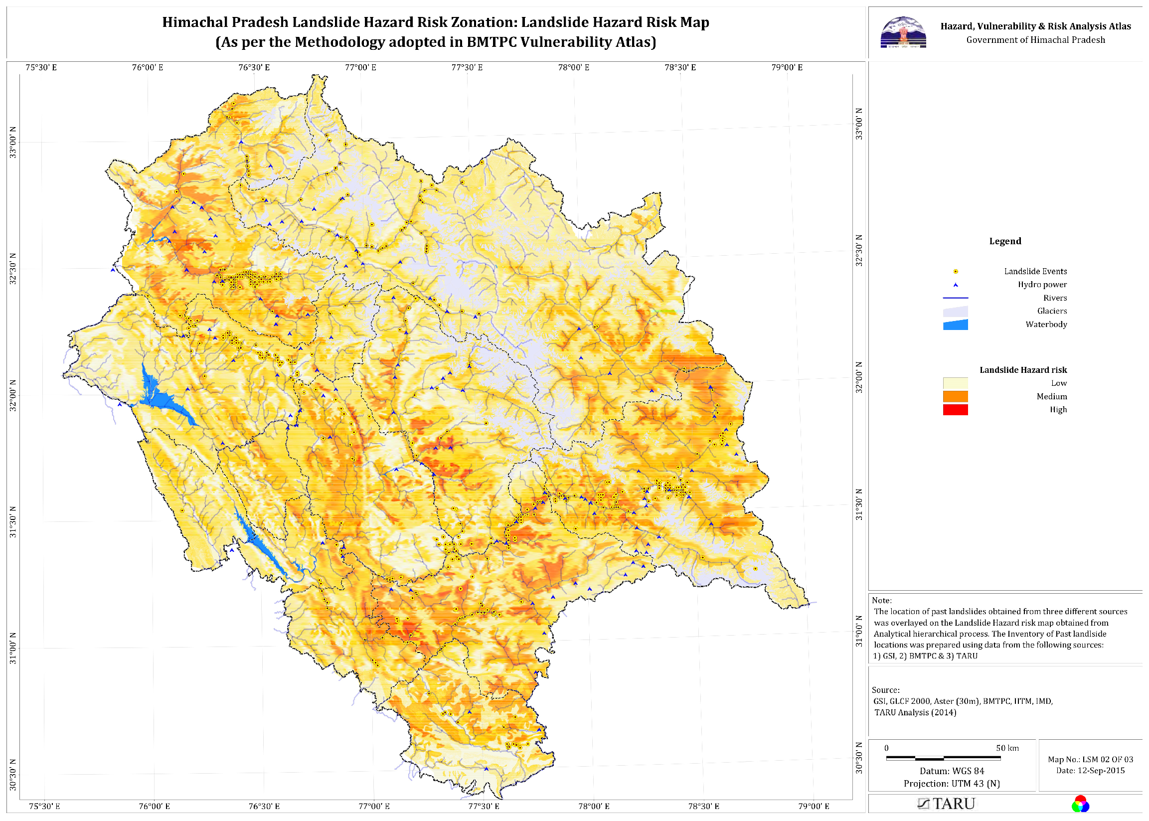
Landslides are a common occurrence during the rainy season, resulting in human, animal, and property losses and obstructing the area’s transportation facilities. Himachal Pradesh, a hilly state in north India, is plagued by landslides that frequently recur, making this study essential [1]. Several instances of landslides caused by rain that damaged infrastructure in various nations, including Italy and Central America [2,3]. A global database of landslides inferred that approximately 75% of the non-seismic landslide occurred in Asian regions when analyzing the data between 2004 to 2016. Most landslides occur in the Himalayan region [4,5]. The need and significance of this study are graphically depicted by the landslide hazard and risk zonation map of Himachal Pradesh (Figure 1).
Rainfall acts as the main triggering factor for landslide; the Himalayan region’s new folded mountains and seepage adversely affects slope stability, causing an increased number of slope failure during the monsoonal season [5,6,7]. The relationship between rainfall and landslide has been widely discussed [8,9,10]. Researchers have developed a threshold-based approach to assess the occurrence of landslides. Various methods can assess these thresholds: empirical methods [11,12], probabilistic methods [13,14,15,16], and mathematical methods [17,18]. With the advancement in technology, there are other tools, such as geological information systems (GISs) and Global Positioning Systems (GPSs) based on remote sensing and satellite data that can be used to develop a hazard zonation map [19,20,21,22] and to identify landslides through automatic process and calculation [23,24]. These methods require a skilled team for deployment, which increases the cost. They are suitable for a regional or larger area for early warning, which requires a large amount of data, without which could result in a false alarm. Physical model methods are best suited to analyse the mechanism of rainfall-induced landslides for individual slopes due to their unpredicted nature and various triggering factors [25,26,27,28]. Numerical modelling methods are widely known to analyse the stability and seepage parameters for individual slopes, as it is not feasible to perform a physical model test for every individual slope due to its complex setup and procedure [29,30,31,32,33,34,35]. In [36], the study used physical and numerical modelling to analyse the rainfall-induced landslide and validated the numerical modelling results with physical modelling. However, the above methods can be combined for hazard risk zonation and to identify the critical slope. It can be seen that sometimes a steeper slope remains stable, whereas a gentle slope may fail under critical conditions. Keeping this in mind, it is important to consider individual slope monitoring for early prediction. As rainfall-induced landslides show the unpredictable nature of failure than the landslide initiated by the effect of gravity, scheduled field inspection at regular intervals may not be an effective method [37]. With the advancement in electronic components and wireless networks, in situ ground-based monitoring of slopes is another emerging method for real-time monitoring of slopes. These methods are also suitable for places not suitable for frequent visits. Different equipment and sensors are used for monitoring and predicting for ages. Extensometers are used to find the displacement of the moving slope with respect to a stable portion [38]. However, this method needs extreme precision in selecting the critical slip surfaces to be installed. Inclinometers are also used to monitor deep-seated landslide [39,40] as well as slow-moving earth flow [41] but the installation and maintenance costs are much higher, and thus cannot be suitable for low-cost purposes. The use of tilt sensors for the detection and monitoring of critical slopes is widely known due to its cheaper development and installation costs, and are found to be effective in monitoring shallow slope failures [42,43,44]. This technique was developed and successfully tested in Japan [43,45] and is now widely accepted by various countries for its low cost and efficient performance alternative to the traditional extensometers and inclinometers. The geology and hydrological pattern of the Indian Himalayan region are very different from the location where these sensors have already been used, thus requiring performance evaluation before installation.
Himachal Pradesh in the Indian Himalayan region is one of the states in Indian territory that is vigorously affected by landslide events yearly, and the number increases every monsoonal season. These events severely affect the life and property in nearby communities [6] as these regions come under the newly folded mountains, which are eventually affected by various landslides due to the infiltration and pore pressure that develop between the soil pores. Only a few researchers have used tilt sensor-based techniques to monitor the critical slopes in the Indian Himalayan region. Some studies [42,46] used tilt sensors in Darjeeling Himalayas for monitoring slopes, but very few can be found in the Himachal Himalayas region, proving this area is open for further research. In this study, a cost-effective monitoring system has been developed using Micro Electro-Mechanical System (MEMS) sensors. A volumetric water content sensor has also been used in order to study the role of the rainwater effect. The laboratory physical modelling method has been used to evaluate the performance and working efficiency. By integrating multiple sensor technologies and using advanced data analysis techniques, it is hypothesised that a landslide monitoring system can be developed that will provide accurate and timely information about landslide activity, thereby reducing the risk of property damage and loss of life caused by landslides. This study can provide cost-effective monitoring of slopes and the development of early warning systems for rainfall-induced landslides so precautions can be taken to lessen their impact.
2. System Design and Implementation
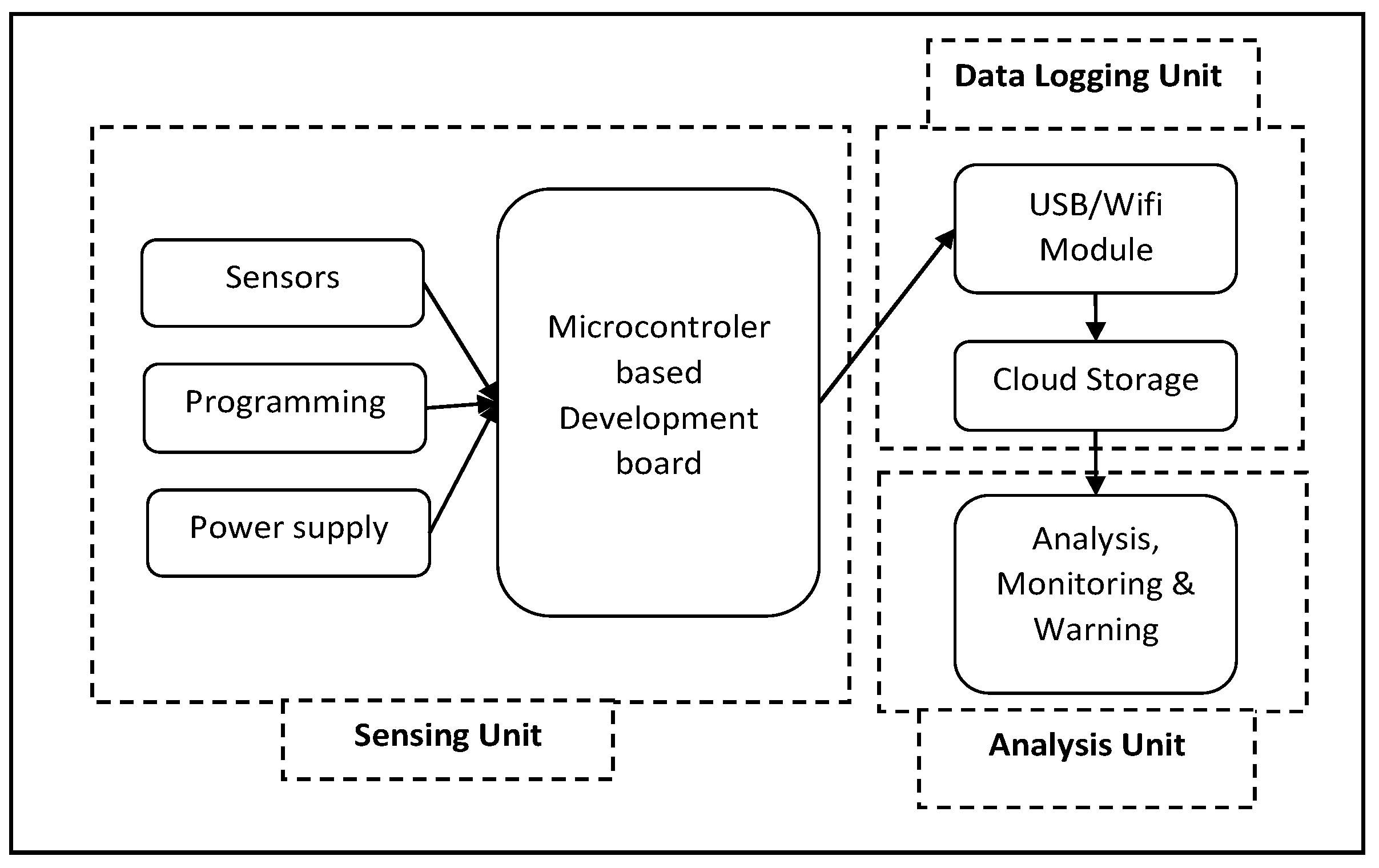
The design of the proposed landslide monitoring system consists of three major components: a sensing unit which includes the sensors and microcontroller, a data logging unit, including a connection and networking module for the collection and storage of data, and a threshold analysis unit, which can be helpful in generating the warning. Figure 2 shows the schematics of the proposed system.
2.1. Sensing Unit
The sensing unit is the first and foremost part of the proposed system for monitoring landslide initiation. It includes the sensors used to sense the required data for the analysis. This system uses Micro Electro-Mechanical System (MEMS)-based sensors for their efficient working, durability, and cost-effective availability. This system will be deployed in the field and cannot be reused if a landslide takes place, making MEMS-based sensors suitable for this purpose. In this study, the components that were used are discussed below.
2.1.1. Tilt Sensor
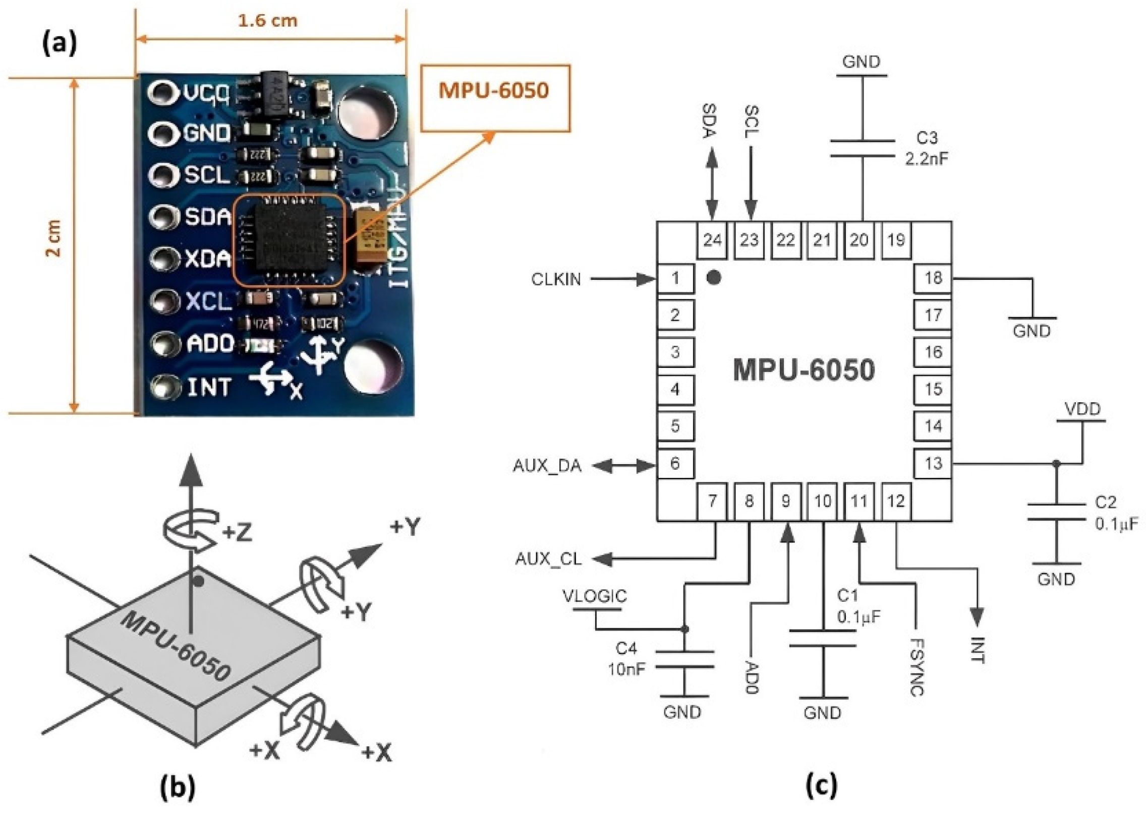
It is necessary to choose a module (MPU6050), which consists of an accelerometer, gyroscope, and temperature sensor, to record the tilt variation in the x, y, and z directions. The 16-bit triaxial gyroscope and accelerometer are combined into the six-axis sensor.
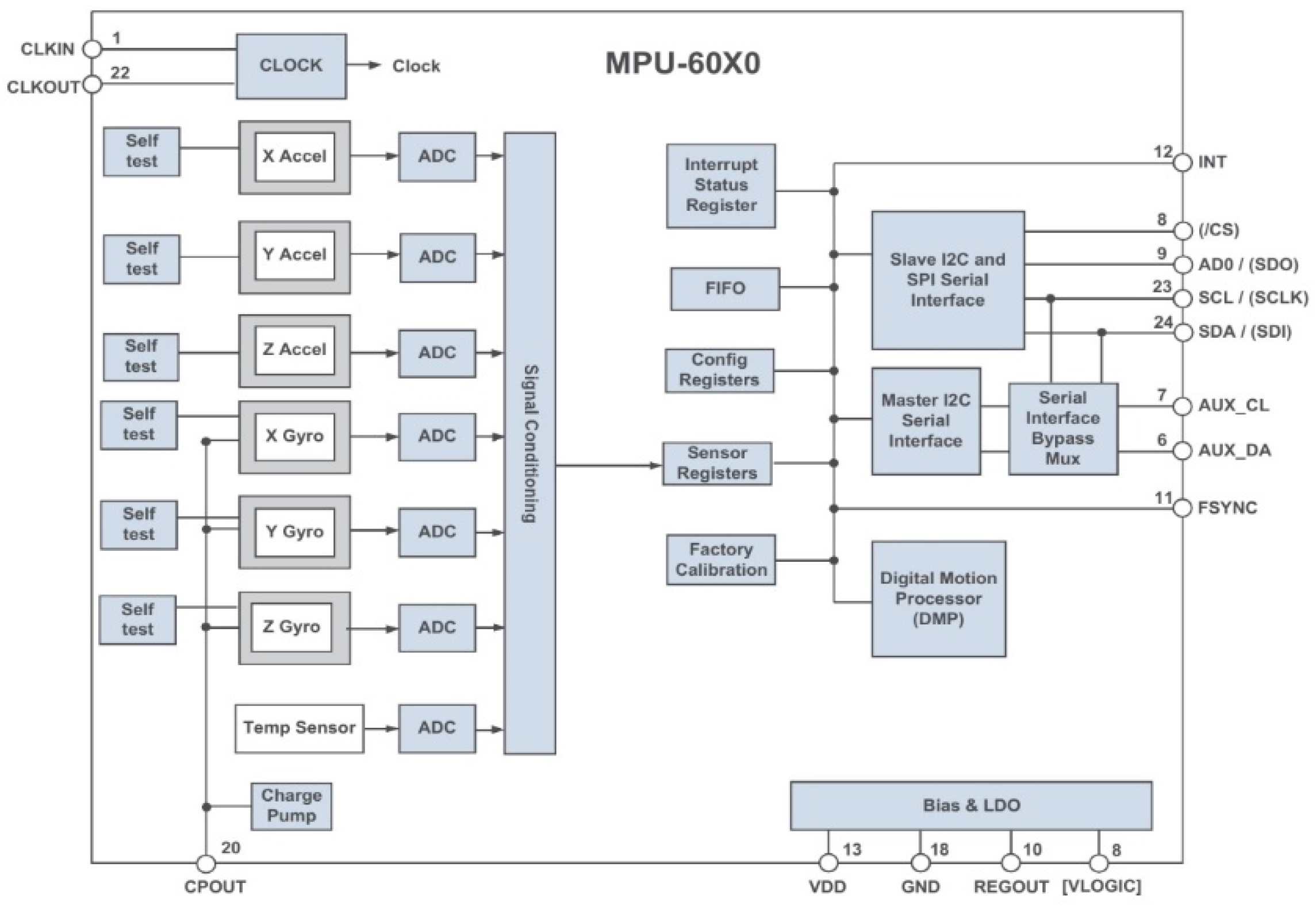
The module is built around an MPU6050 InvenSense IMU (Inertial Measurement Unit) chip. It comes in a PCB board with a 2 cm × 1.6 cm dimension and 24 pins. An AP2112 K 3.3 V regulator, I2C pull-up resistors, and bypass capacitors are some of the few components that make up the module, which has a meager component count overall. In addition to this, there is a power led that displays the current power status of the module (Figure 3a). The MPU6050 is a Micro-Electro-Mechanical System (MEMS) that contains within it a three-axis accelerometer as well as a three-axis gyroscope (Figure 3b). This allows us to measure the acceleration, velocity, orientation, and displacement of a system or object, in addition to a wide variety of other motion-related parameters. This module also contains a Digital Motion Processor, abbreviated as DMP, capable of carrying out intricate calculations and relieving the Microcontroller of some of its responsibilities. Figure 3c explains the circuit diagram, and Figure 4 shows the block diagram of the MPU6050 module for a better understanding of the working of the sensor.
MEMS accelerometers are used in situations where there is a requirement to measure linear motion, such as movement, shock, or vibration, but there is no fixed reference point. They track the object’s linear acceleration while being tethered to it. The mass on a spring principle is the premise on which all accelerometers operate. Due to inertia, the mass seeks to remain immobile as the item to which they are attached accelerates. As a consequence, the spring undergoes stretching or compression, resulting in the production of a force that can be measured and is related to the acceleration that was applied. In a MEMS accelerometer, a pair of silicon MEMS detectors made of spring-“proof” masses are used to precisely detect linear acceleration in two orthogonal axes. Every mass supplies a moving plate with a variable capacitance made up of a variety of interlaced finger-like structures. Due to the proof mass’s tendency to resist motion when the sensor’s sensitive axis is linearly accelerated, the mass and its fingers are forced away from the fixed electrode fingers. An effect of dampening is produced by the gas between the moving and fixed silicon fingers. This displacement causes a differential capacitance inversely proportional to the applied acceleration. A high-resolution analog-to-digital converter (ADC) is used to measure the change in capacitance, and the acceleration is then calculated using the rate of change in capacitance. This is then transformed into a readable value in the MPU6050 before being sent to the Inter-Integrated Circuit (I2C) master device.
The MEMS gyroscope’s function is based on the Coriolis Effect. According to the Coriolis Effect, when a mass moves with velocity in one direction and is subjected to an external angular motion, a force is created that pushes the mass in a perpendicular direction. The amount of angular motion used has a direct impact on the rate of displacement. Four proof masses are included in the MEMS Gyroscope, which is kept oscillating continuously. The Coriolis Effect alters the capacitance between the masses when an angular motion is applied, depending on the direction of the angular motion. A reading is created after this change in capacitance has been detected.
2.1.2. Soil Moisture Sensor
Unquestionably, water is crucial to the chemical, physical, and mechanical characteristics of the soil. Understanding and analyzing various processes involving soil, vegetation, and atmospheres, such as soil erosion, runoff, and soil water infiltration, depend on quantifying soil water content from the surface to greater depths. Due to the ability of aerial plant life to capture some of the water that falls as rain and the ability of plants to absorb moisture from the soil around them and release it to the atmosphere through evapotranspiration, soil vegetation alters the hydrological balance of the affected area. The latter mechanism could result in a decrease in the saturation level of the soil (an increase in suction), which would increase the soil’s shear strength. In other cases, water accumulation between the soil layer can cause the formation of the fluid zone, which may lead to a loss in shear strength which may lead to slope failure [47]. Thus, soil vegetation plays a vital role in stabilizing the slope to protect the environment.
With the help of this sensor, it is possible to track changes in soil moisture continuously. The soil moisture sensor consists of two probes to measure the volumetric water content by measuring the resistance or capacitance value through the soil material. The change in current or voltage is then calibrated to measure the water content. When the soil pores have more water, the resistance to current flow will be less as water provides better conductivity. Similarly, when less water is present in the pores, the resistance offered by the medium will be very high, reducing the current flow due to the poor conductivity offered between pores.
Compared to other sensors on the market which measure resistance, in this study, a capacitive soil moisture sensor version 2.0 is used to measure soil moisture levels through capacitive sensing. Version 2.0 has a better upgrade and offers a better service life than previously available versions, as it is corrosion-proof. The output of the capacitive moisture sensor is known to be influenced by the complicated relative permittivity () of the soil, i.e., dielectric medium [48,49].
where, and are, respectively, the real and imaginary components of permittivity, referred to the electrical conductivity, is the contribution of molecular relaxation (dipolar rotation, atomic vibration, and electronic energy states), indicates the imaginary number √ (−1), and is the frequency. The amount of energy from an external electric field that is stored in a material is measured by the real part of permittivity (). The “loss factor”, also known as the imaginary part of permittivity (), predicts a material’s susceptibility to dissipation or loss in the presence of an external electric field: > 0. Losses are linked to two main processes: electrical conductivity and molecular relaxation. The soil’s salinity, ionic composition, frequency, and moisture affect permittivity.
The permittivity of a material is often represented by a complex number with a real part and an imaginary part. The real part of the permittivity represents the material’s ability to store electric charge, while the imaginary part represents the material’s ability to dissipate electric energy.
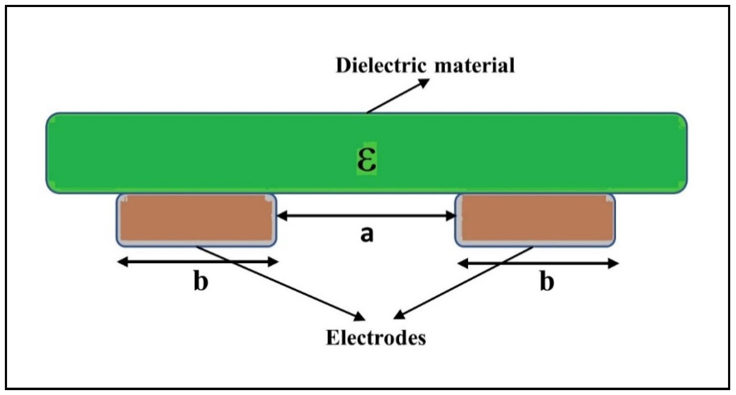
Capacitive soil moisture sensors utilise the operation of a capacitor to provide an approximation of the amount of moisture present in the soil. The amount of charge a material can hold when subjected to a specific external electrical potential is referred to as its capacitance [50,51]. The most common way to conceptualise capacitors is as parallel-plate setups, as shown in Figure 5 below.
The capacitance of an object can be expressed as a ratio of its charge to its electrical potential:
The charge Q defined by the integrating relationship between the generated electric field (E) and the relative permittivity of the surrounding dielectric material (ε) throughout the gross surface area of the probes. The line integral of the electric field is used in the definition of electric potential, abbreviated as V. is the distance between plates. For the capacitor with parallel plates, an assumption can be made that the electric field is uniform throughout the whole surface of the dielectric. This leads to the resulting simplification:
This is usually believed to represent the relationship between the geometric parameters of a capacitor with parallel plates and the soil material having dielectric properties around the capacitor. The capacitance measured by a soil moisture sensor is distinct from that recorded by a capacitor with parallel plates, as the capacitor plates are coplanar rather than parallel. This indicates that the plates are not stacked on top, but are placed adjacent to one another and that the dielectric substance is the ground itself instead of a thin layer trapped between the plates. The following illustration demonstrates this point.
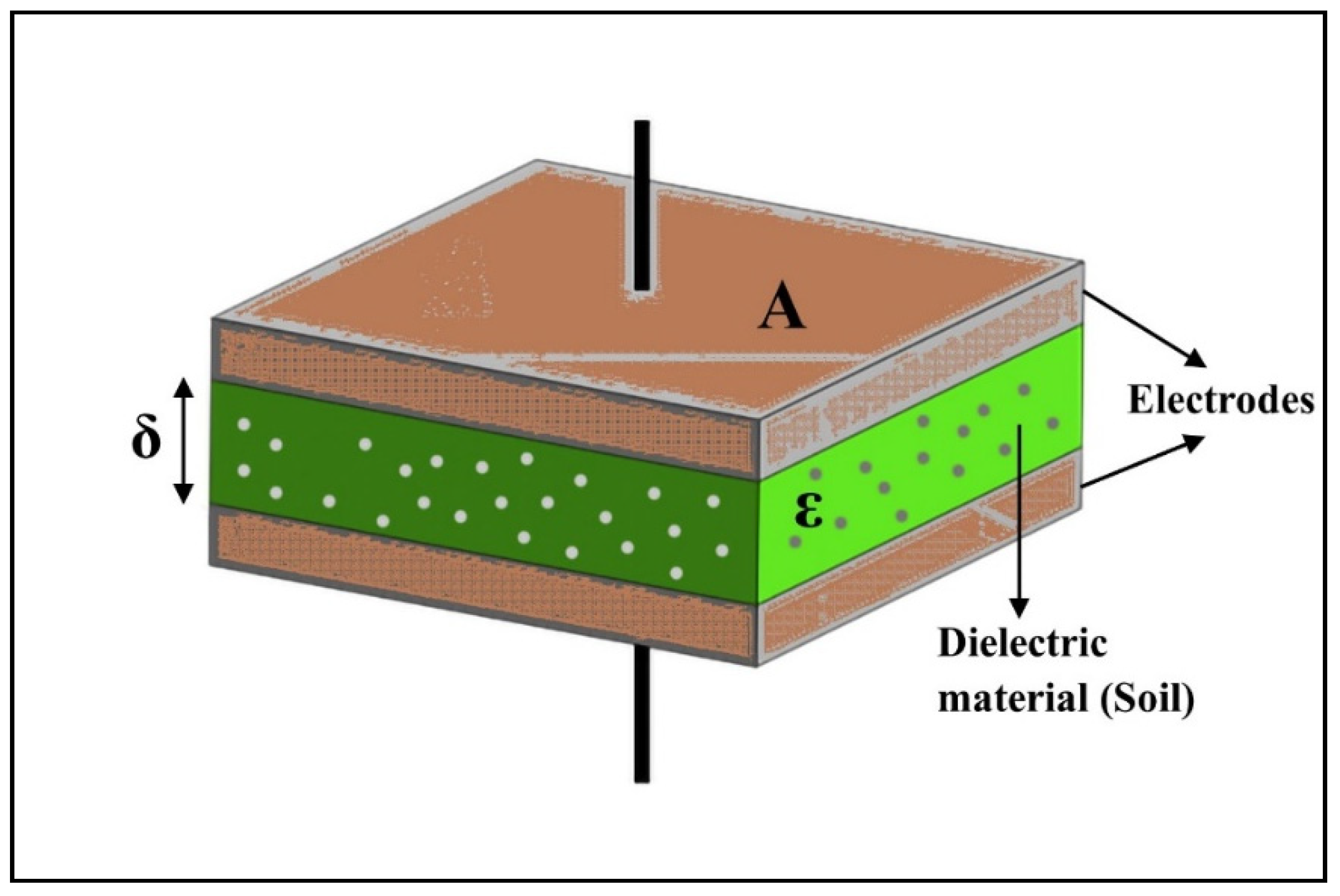
Figure 6 clearly shows the arrangement of electrodes with the dielectric medium, which can be dry or wet soil and serves the same function similar to the plates of any capacitor. The capacitive soil moisture sensor works in conjunction with a timer circuit (TLC555, in the case of the selected sensor). The combination produces a duty cycle proportional to an analog voltage. This voltage can be read off using a built-in microcontroller board. Capacitance for a flat capacitor is a complex function of dielectric constant and sensor shape that will not be investigated here. The only new component that has been added is G, a function that summarises the geometric qualities of the sensor. The relationship is shown in Equation (4).
The geometrical and dielectric medium, along with surface line integration in planer configuration, makes the complex function, which can be simplified for better understanding by assuming a constant (A) as shown in Equation (5), and the solution to finding the dielectric constant is mentioned in Equation (6).
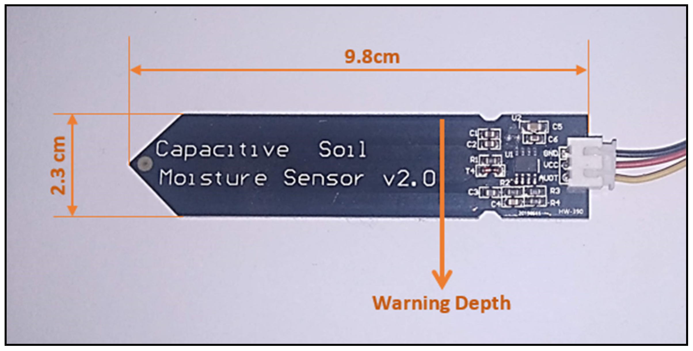
In essence, this indicates that a correlation between the dielectric constant and the inverse of the voltage received by the sensor can be anticipated. Using the above relationship, the soil moisture sensor is calibrated to sense the moisture in soil pores in percentage or as the volumetric water content. Figure 7 shows the chosen, commercially available blade-shaped Capacitive Soil Moisture Sensor v2.0.
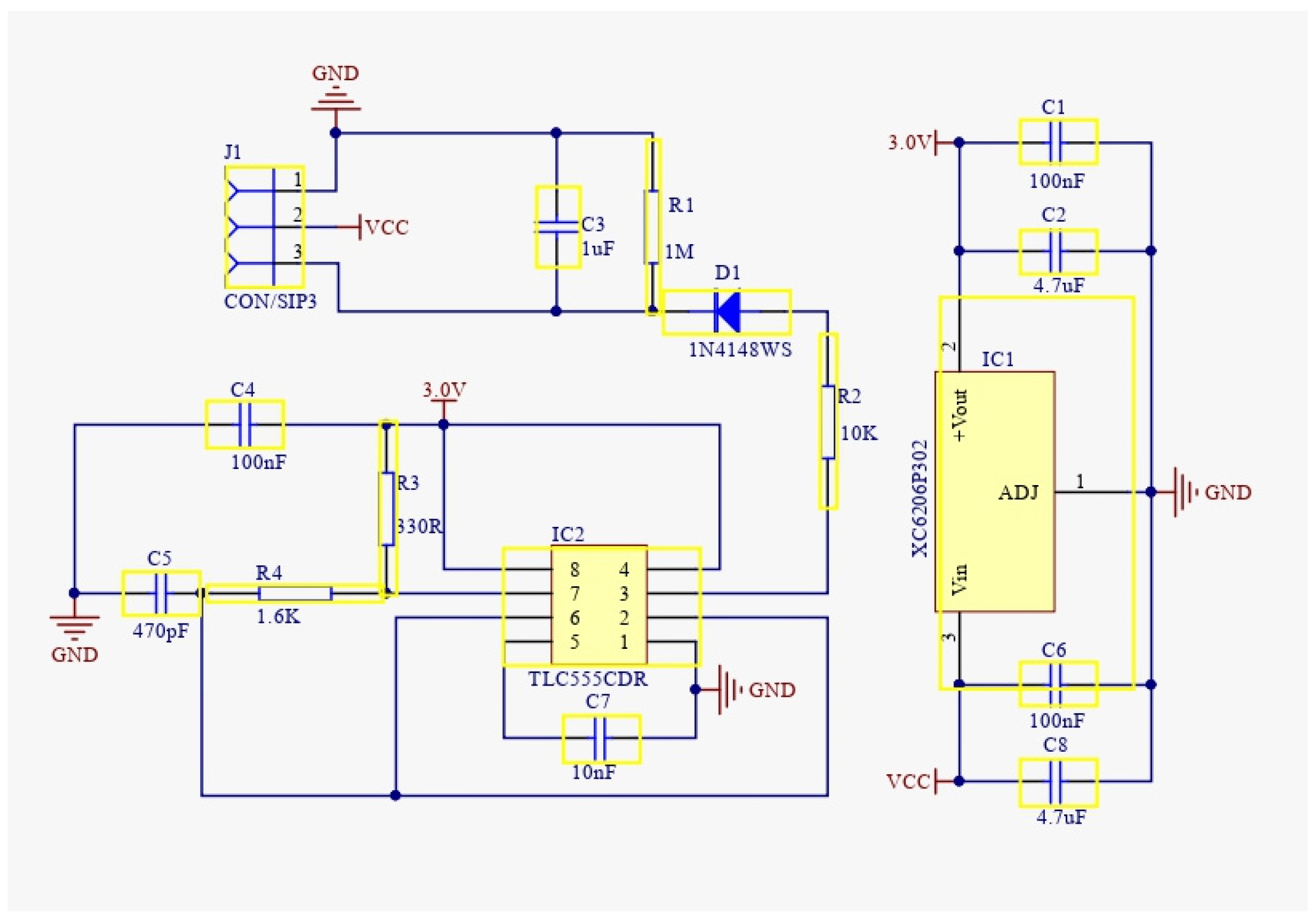
The most recent and reliable information for the version 2.0 soil moisture sensor developed by DFROBOT and sold under the SKU (stock keeping unit) designation of SEN0193 in various advertisements [52]. The datasheet suggests a suitable depth of penetration in soil, a working power supply between 3.3 and 5.5 volts, and an output voltage between 0 and 3.3 volts. Initially, a comprehensive investigation into the sensor’s electrical circuits was carried out to become familiar with the functioning mechanism. The circuit diagram of the soil moisture sensor from the datasheet is shown in Figure 8.
2.1.3. Development Board
The development board is like the heart of the monitoring system, as all the necessary parts are connected. The panel includes a microcontroller for reading and processing sensor values. The board consists of an input pin for analog and digital sensors, a power supply connecting headers, and a USB port to transfer the data. It can also be combined with various modules, like the Wi-Fi module, to transmit the data to the cloud or the memory card module to store it for further analysis.
2.1.4. Power Supply Unit
The power supply unit includes the power supply for all modules in the monitoring system. It consists of a battery with enough capacity of 10 k mAh for the uninterrupted working of the system and a solar panel charging system for continuously charging the battery. The solar charging system was equipped with the overcharging protection of the battery to ensure the longest battery life.
2.1.5. Programming
Programming is the soul of any monitoring system. It communicates a program’s intended functionality to a computer through a sequence of instructions. In this system, two types of sensors were used to monitor the landslide mechanism. Programming for the MPU6050 sensor was done to compute the tilt angle, and any deviation induced by tilting can be recorded with time. The system has the capability to adjust itself by restarting to allow for better visualization. The second sensor was installed to monitor the volumetric water content of the soil, and programming was done to measure the moisture content in terms of percentage with time.
2.2. Data Logging Unit
This unit ensures the data collection acquired by the sensor. The data logging module can be attached to the development board using the USB hub or the memory card module to save the data. A Wi-Fi or GSM module can also be connected wirelessly to collect the sensor value on the internet cloud for further analysis. The development board is equipped with a Wi-Fi module to provide internet connectivity in the developed monitoring system. A GSM-based Wi-Fi modem was installed so that several monitoring sensors could be connected using the single modem according to the slope area and location, reducing the cost of individual GSM modules and the connectivity charge. The data collected from the sensors were stored using the Arduino cloud for further analysis.
2.3. Analysis Unit
In this section, the data collected from the sensors are analysed for better monitoring of slope movement. As the critical threshold value depends upon the geometry and material of the slope, it varies for individual slope. After sufficient analysis and monitoring, a warning can be generated for each slope to reduce the catastrophic effects of slope failure by evacuating or strengthening stability.
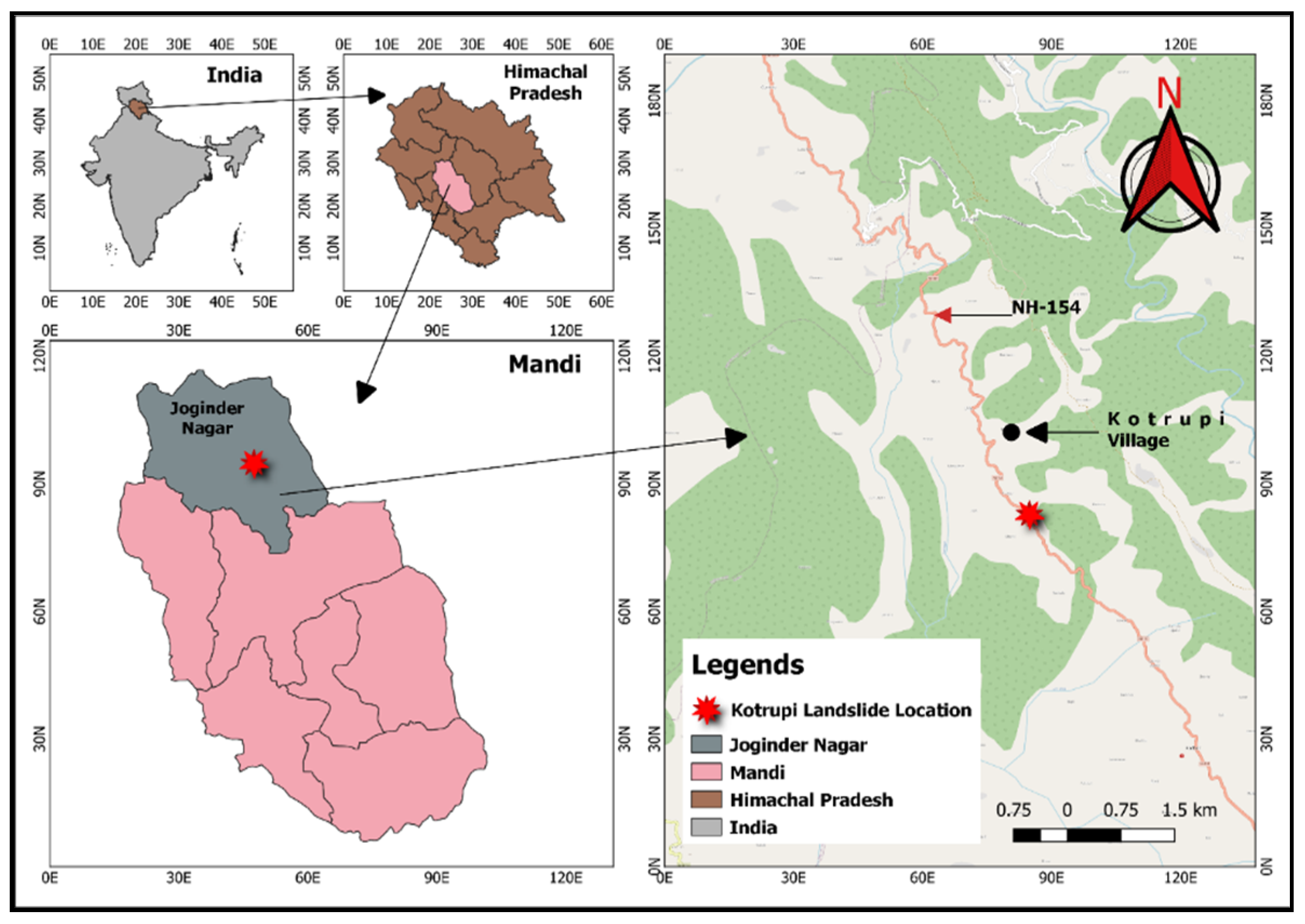
3. Study Area
The study location (Figure 9) is in the vicinity of Kotrupi village on the Mandi—Joginder Nagar—Pathankot National Highway (NH-154), where the Kotrupi landslide has caused extensive damage [53]. On either side of the slide, the Padhar and Joginder Nagar tehsils of the Mandi district (Himachal Pradesh) are approximately 4 and 21 km away, respectively. The study area is covered by the Survey of India Toposheet No. 53 A/13. Geographical coordinates with latitude N31°54′37.60″ and longitude E76°53′26.30″ indicate the location of the landslide [53].
3.1. Landslide Event and Mechanism
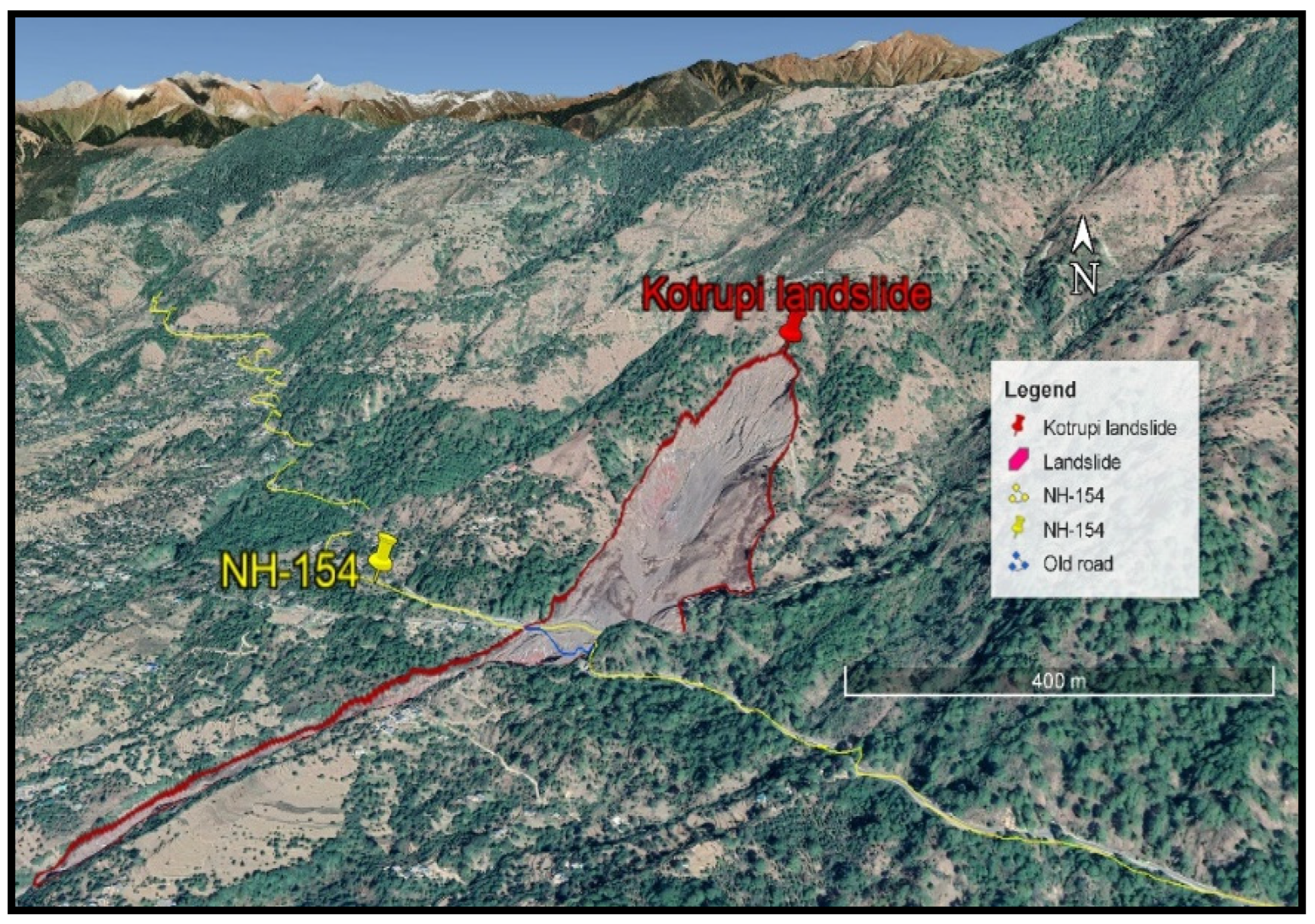
On Sunday, 13 August 2017, a major landslide happened in the Mandi District of Himachal Pradesh in the village of Kotrupi (near the Kotrupi Bus Stop). The road connecting Mandi and Pathankot was affected by the landslide. According to reports, a section of the slope completely collapsed, burying two Himachal State Transport buses and a few other cars, and at least 47 people were killed in the tragedy [54]. Nearly three hundred meters of the highway were entirely buried by debris, shutting off contact on a vital corridor. There have been scars from small landslides in the Kotrupi region prior to the actual landslide. Debris flow slides occur when significant soil mass has flowed down a steep channel with debris. The Kotrupi landslide was one of the types of debris failure [54].
3.2. Description of Study Slope
The area includes part of the catchment basin of the Beas river, and several tributaries join it. The Uhl river, Rana Khad, Arnodi Khad, and Luni Khad are minor tributaries of the Beas River. Physiographically, the area falls in the Lesser Himalayan Zone occupied by the Dhauladhar range in the northeastern part. The topography is rugged, displaying high ridges and deep valleys. Figure 10 shows the satellite view of the study area, indicating landslide crown and runout. The slope is moderate to steeply inclined with occasional breaks in the slope. The slope is moderately to highly dissected, as evidenced by minor streamlets on either side of the slope. The slope affected by the failure has a 45°–50° inclination. The landslide’s crown is located at an elevation of 1620 m. The main landslide is approximately 230 m tall, with a 210 m width. The slide is 300 m long from top to bottom. The landslide’s runout distance was 1155 m [54,55].
3.3. Geotechnical Characteristics of the Slope Material
Slope-forming material was collected during the field survey to find the hydromechanical and geotechnical parameters. In order to minimise the differentiability of location in the simulation of the material properties and to better understand the Kotrupi landslide’s behaviour, materials were collected at various locations throughout the landslide area. Grain size analysis, Atterberg limits, natural water content, specific gravity, a compaction test, and a triaxial test were carried out using the disturbed samples taken from the site per the IS code. The material can be simulated in numerical modelling using the outcomes from experimental investigations. After performing grain size analysis, the material was categorised by three fractions, i.e., sand, silt, and clay. The material collected from the site was classified as a non-uniform gradation because it contained a wide variety of possible particle sizes, including plants, big stones, and boulders. Indian standard code IS: 2720 was followed to perform sieve and hydrometer analyses to determine grain size [57], and the results showed the values of coefficient of uniformity Cu is 6.2 and coefficient of curvature Cc as 0.67. The fineness modulus of the material was found to be between 5 to 12 percent, and the soil was classified as poorly graded sand containing less amount of silt (SP-SM). To perform seepage analysis to investigate the pore pressure parameters, the determination of Atterberg’s limit is an essential parameter in material simulation [58]. Indian standard code IS:2720 (part 5) was used as a reference to perform Atterberg’s limit tests [59]. Atterberg’s limit results are summarised in the Results section of the paper. IS code: 2720 (Part-7) was referred to perform light compaction tests to determine the dry density of the soil [60]. According to the geotechnical investigation performed during the laboratory investigation, the material obtained from Kotrupi landslide location mostly contain poorly graded sand (SP). The landslide’s shear strength parameters can be calculated using either the drained or the undrained stresses, the total or the effective stresses [61]. In the case of a debris-type landslide, the unconsolidated-undrained test has been recommended for soil characterization [62]. Following IS: 2720, part 11, the tests were conducted at normal stress of 50 kPa, 100 kPa, and 200 kPa to determine the shear strength parameters (cu and ϕu) because the soil sample contains some silt [63].
4. Methodology
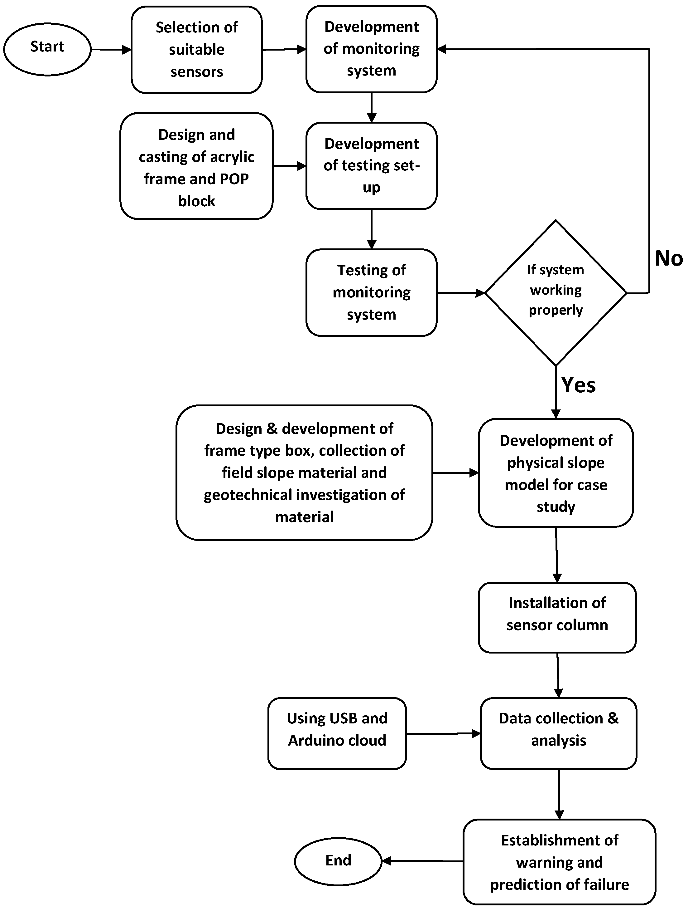
In this study, a low-cost monitoring system that comprises a MEMS-based tilt sensor and soil moisture sensor is developed to investigate the slope movements monitoring the tilting behaviour. A self-made testing platform was designed to test the working of the monitoring system. A soil slope model was prepared in the laboratory to assess how well the sensor works under real-world conditions, including a self-developed rainfall generator to simulate the rainfall. The physical model test is also helpful in investigating the cause and the failure pattern, which helps establish the critical rainfall threshold. A series of physical model tests were conducted to assess the effectiveness of the sensor column monitoring process by evaluating the applied sensor column deformation behaviour with the observed tilt response. Landslide events have been modeled in two different ways: (i) a direct shear setup simulated first-time landslide failure experiment using a sensor column to analyse the performance of developed system directly with relative deviation in angle; and (ii) by creating a soil slope model to test and monitor the functioning of the monitoring system by simulating real conditions and also to investigate the failure mechanism behind the rainfall-induced landslide by simulating a case study. The study’s methodology flow chart is shown in Figure 12.
4.1. Testing Setup
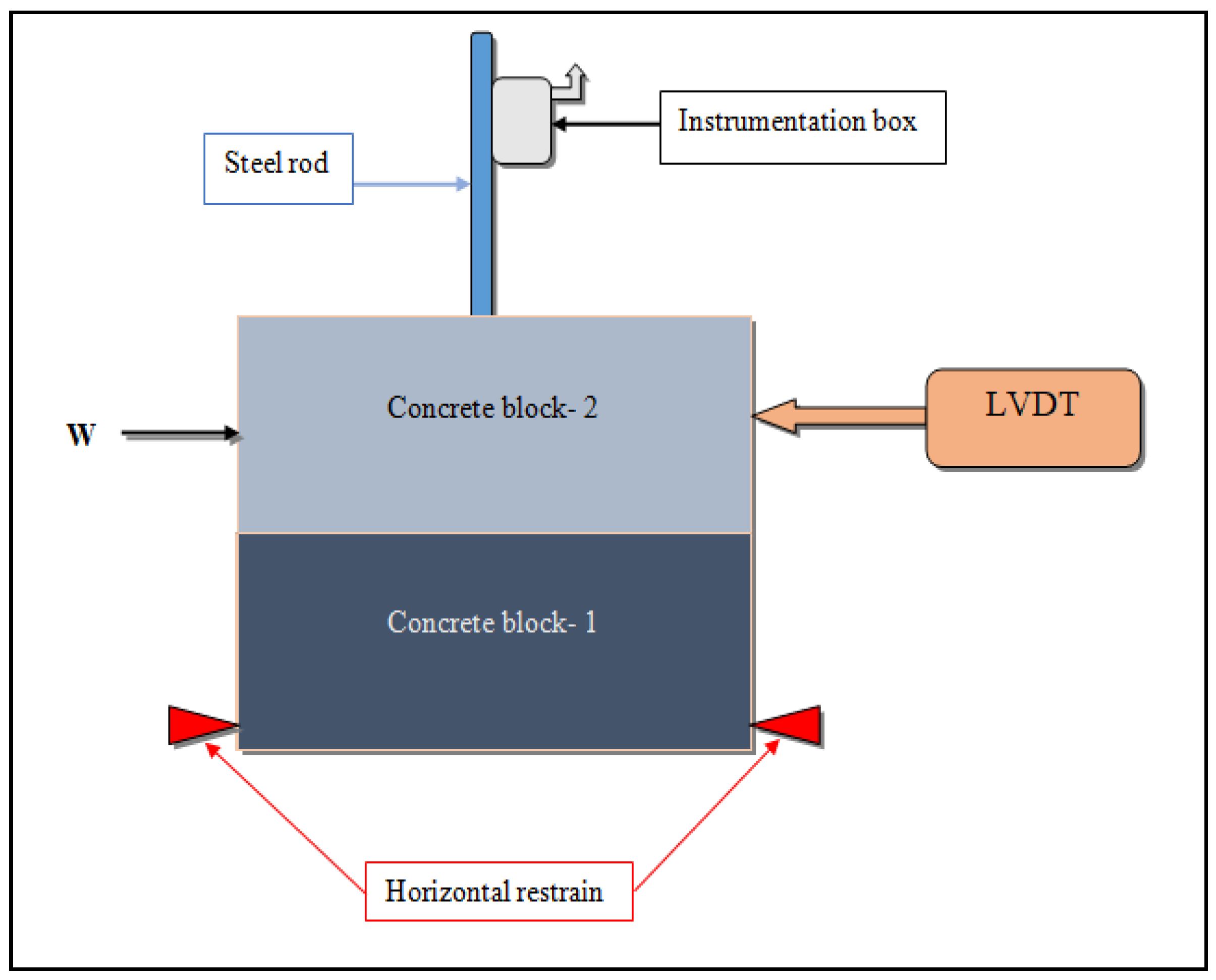
The testing method includes a predefined failure plane to simulate the slope failure plane in order to check the working and performance of the developed system. Figure 13 is a schematic representation of the physical model of a slope failure that was used to analyse the displacement behaviour using a tilt measurement and to accelerate the top box relative to the bottom box. The setup includes a hydraulic jack to create a horizontal movement to the upper block against the fixed wall support. The lower block is fixed to any movement. Both blocks have holes throughout the depth where the sensor column was installed. An LVDT (Linear Variable Differential Transformer) sensor was also installed to measure the horizontal deformation induced by the external force applied by the hydraulic jack.
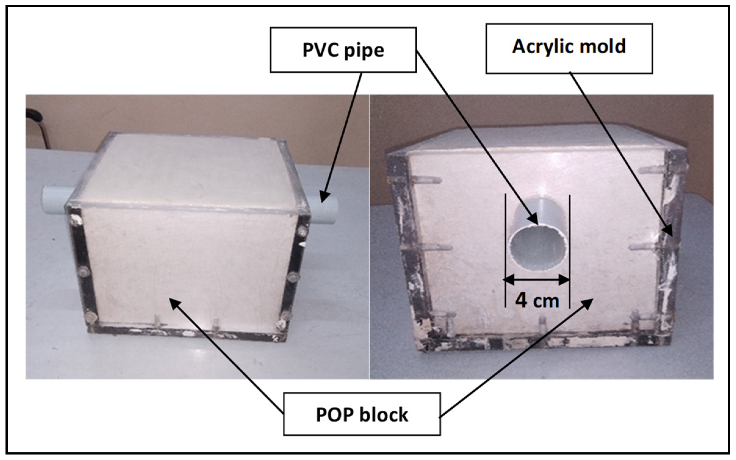
The concrete blocks were made using the Plaster of Paris (POP) material, as it is easy to cast and move around in the lab. The casting was done using a mould of 20 mm × 20 mm × 30 mm made of acrylic sheet, and a hole of 4 cm diameter was made to place a PVC pipe longitudinally to create the borehole in the block for the placement of the sensor column. Figure 14 shows the casted POP block in a casing made of an acrylic sheet of a thickness of 18 mm, and a borehole was created using a plastic pipe of a 4 cm diameter.
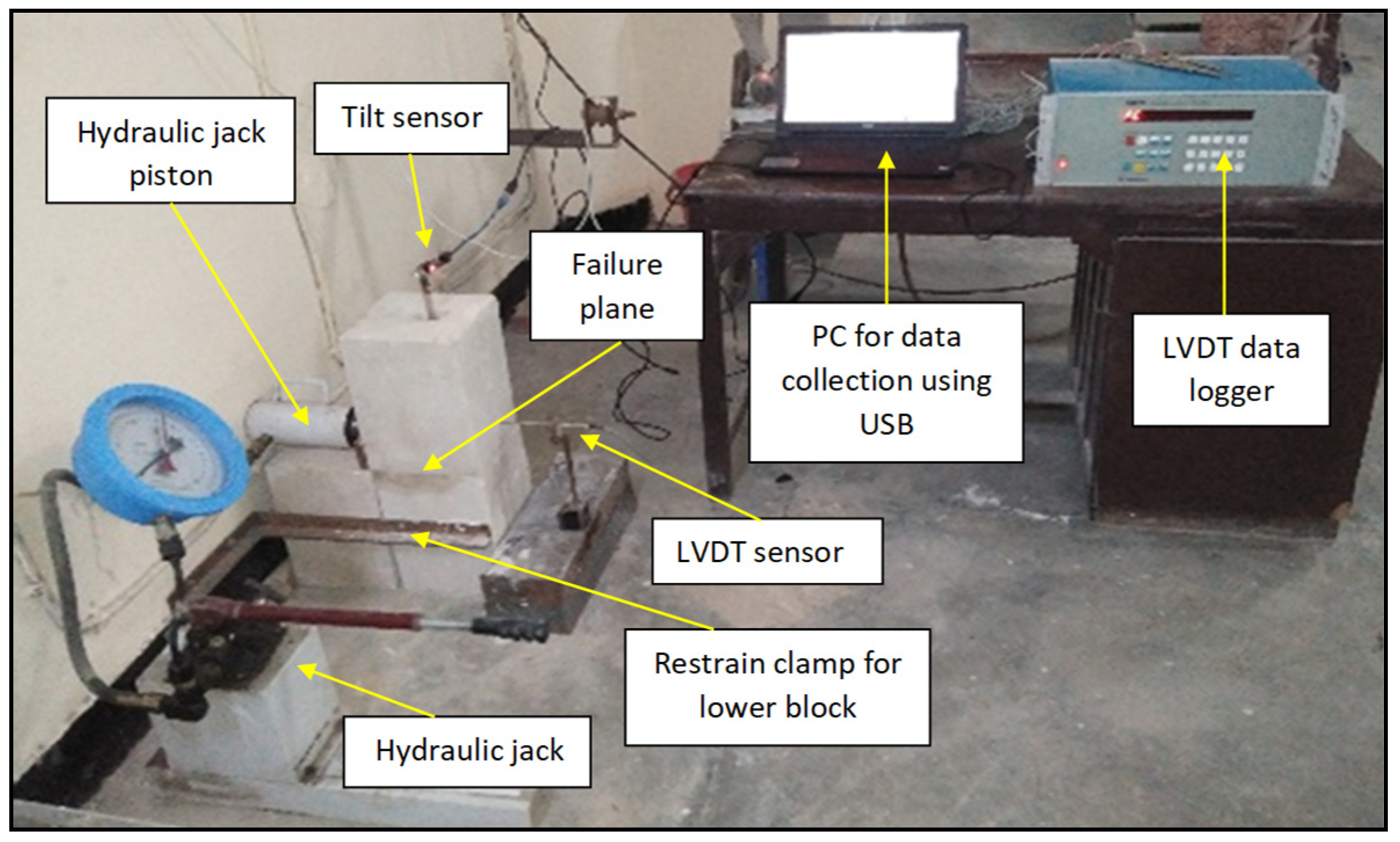
Figure 15 shows the self-made large-scale direct shear model developed using two concrete blocks placed over one another with a bore hole of 4 cm in diameter. The sensor was installed using the steel rod through the column of soil representing the in-situ soil of a slope. The joint made with concrete blocks will act as a predefined failure plane. The lower blocks have been restricted to any movements, while the upper block is free to move when any external force has been applied. The upper block can be considered the failed soil mass, while the lower block is the base of the slab. This sensor was tested by applying an external force with a hydraulic jack to cause a horizontal relative displacement of the top concrete block with respect to the bottom block. The movement change in angle in the x and y directions can be noted for further analysis. The experiment setup was designed so that various tests could be performed to evaluate how well the sensor functions under rapidly changing conditions.
4.2. Physical Modelling of Slope
Debris flows are rapid landslides that pose a threat to human life and property because of their speed and the destruction of infrastructure along their path. Debris flows usually start on hillsides or mountains, most likely when recent rainfall occurs. The rapid collapse, complexity, and random behaviour of debris flow make it difficult to explain the mechanism using a numerical or mathematical model [27]. Therefore, the most common and efficient technique for investigating the slipping mechanism of soil slices utilised in studies of slope collapse is a physical model test, to study the rainfall-induced slope instability, to monitor for potential landslide danger, and to take preventative measures before they occur [27,64,65].
The physical modelling was carried out based on the following presumption. The engineering qualities of the parent soil and experimental soil are the same. There is nowhere for the water to leak except the toe drain because all the sides are impermeable. The sprinkler utilised is not a jet type, so direct rain impact has negligible weathering effect on the slope. For the chosen intensity, rainfall is distributed similarly across the entire slope. The effect of plants, roots, and vegetation on slope stability has not been considered.
In the study, identical engineering qualities were used to enforce a physical modelling test [27,36]. Soil’s basic engineering qualities are determined through dimensional testing of analogous materials in a controlled environment. The identical experimental settings of the physical model were adapted to fit similar theories. This research uses an experimental physical model to examine the conditions of landslide initiation and the mechanism of failure caused by precipitation. The experimental setup is depicted in Figure 16.
4.2.1. Frame Type Box
To facilitate experimentation, a steel framework supports a transparent acrylic sheet 15 mm thick that serves as the frame type model. The tank used in the experiments is a cube, measuring 97 × 57 × 49 cm in dimensions. The toe area also features drainage holes for easy removal of any excess water. The frame type of box was placed over a concrete block in order to place a hydraulic jack on the hillside of the slope to provide a tilting mechanism.
4.2.2. Rainfall Simulator
Two primary measurement-based empirical approaches are used to establish its threshold values: (1) Measurements of rainfall for a given occurrence in terms of both intensity and duration (ID), the sum total of rain that fell during the event (E), duration of a rainfall event (ED), and intensity of a rainfall (EI) thresholds (Guzzetti et al. 2008) and (2) antecedent rainfall event [11] that is, the specified amount of precipitation above which a slope would collapse [66,67]. Three factors have been taken into account in this analysis: (a) precipitation intensity “q”, (b) time duration of rainfall event “t” and (c) the time interval between the consecutive rainfalls. Both the duration and frequency of rainfalls change with the passage of time. Total rainfall “Q” is proportional to the product of time duration and the intensity of rainfall “q” as shown in Equation (7).
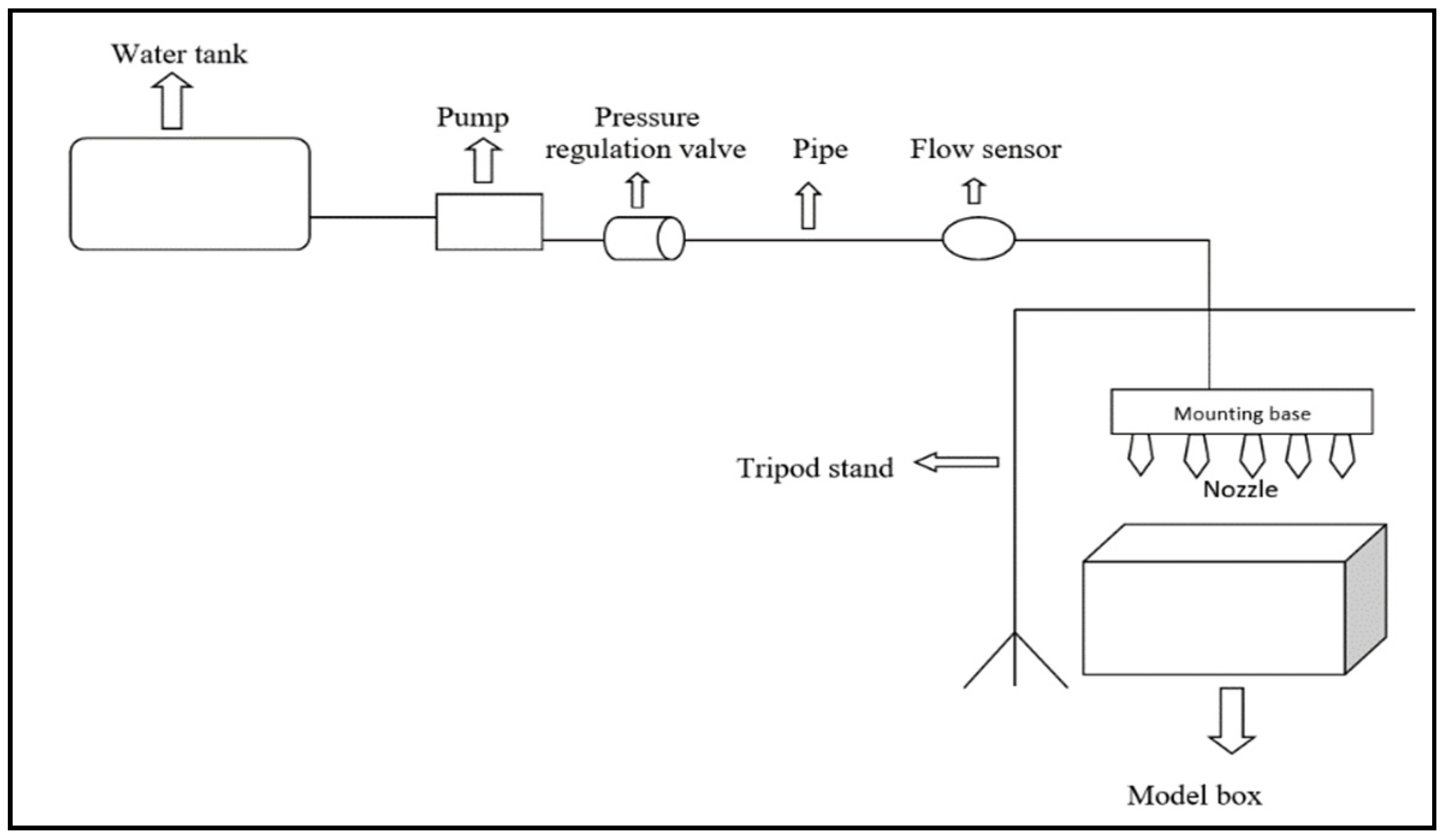
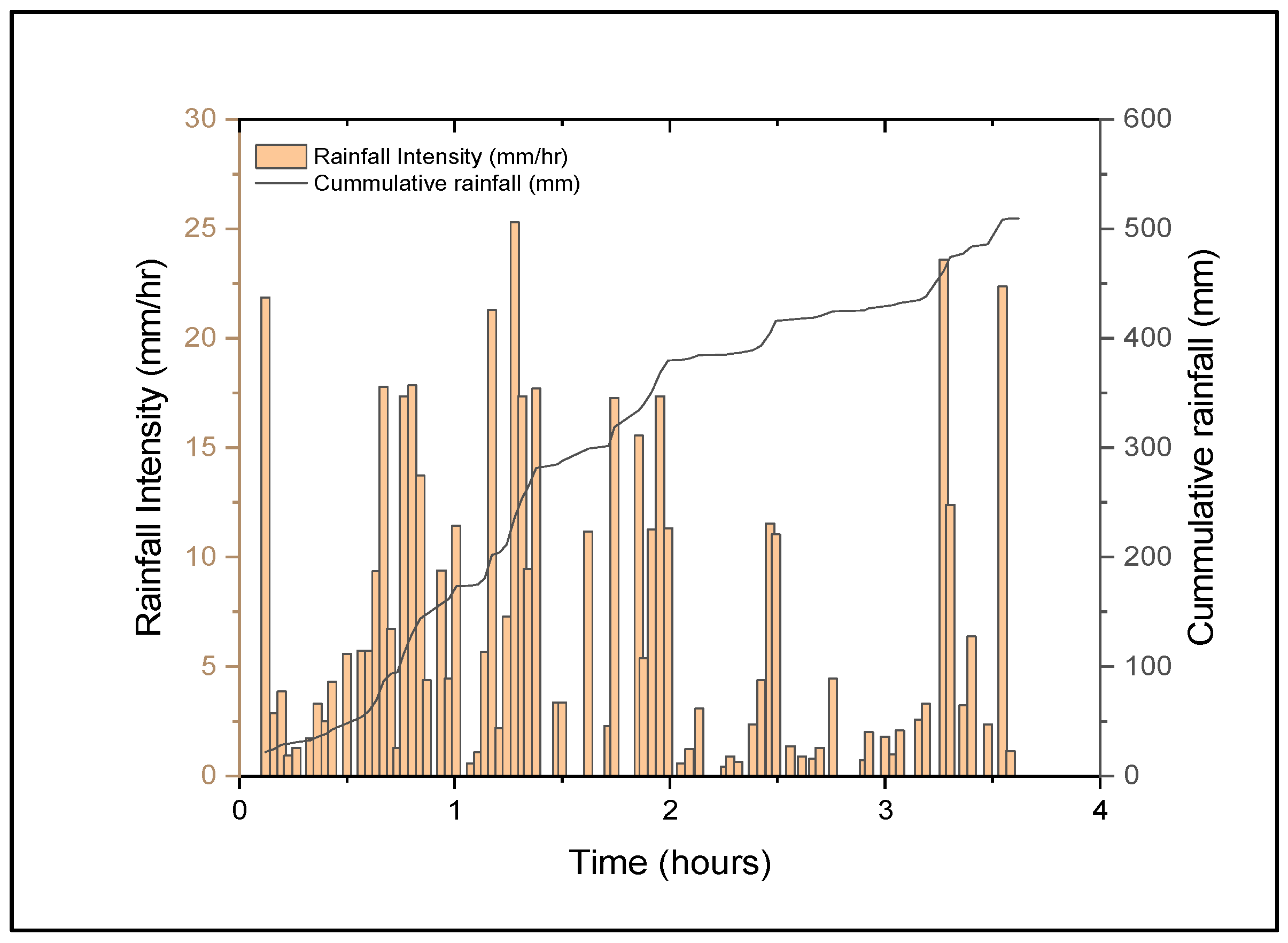
In this study, a self-developed rainfall generator was used to simulate the variable rainfall to simulate a natural environment. An artificial rain generator consisting of a water storage tank, submersible pump, control valve, flow sensor, and raindrop nozzle is constructed to produce the required amount of rain. For the generation of rainfall, several sprinkler nozzles are installed in a rainfall simulator to simulate the rainfall. The nozzle used is a spray type but does have a fixed opening, and the droplet size may vary according to the input flow pressure. The rainfall generator was equipped with a flow sensor that collects the data with a microcontroller. The variable rainfall intensity is attained by controlling the valve attached to the inlet of the rainfall generator. Figure 17 shows the input variation of rainfall intensity and accumulated rainfall depth over time. Variable interval is also introduced after an hour for the next successive rainfalls to make moisture infiltrate properly.
5. Results and Discussion
The findings of this investigation are summarised in this section. The results of the laboratory tests are discussed in greater detail in this article. To better understand the failure mechanism under rainfall, physical slope modelling was used to simulate and investigate the start-up mechanism of the slide. Testing and monitoring results are explained in this section.
5.1. Results of the Self-Developed Test Setup
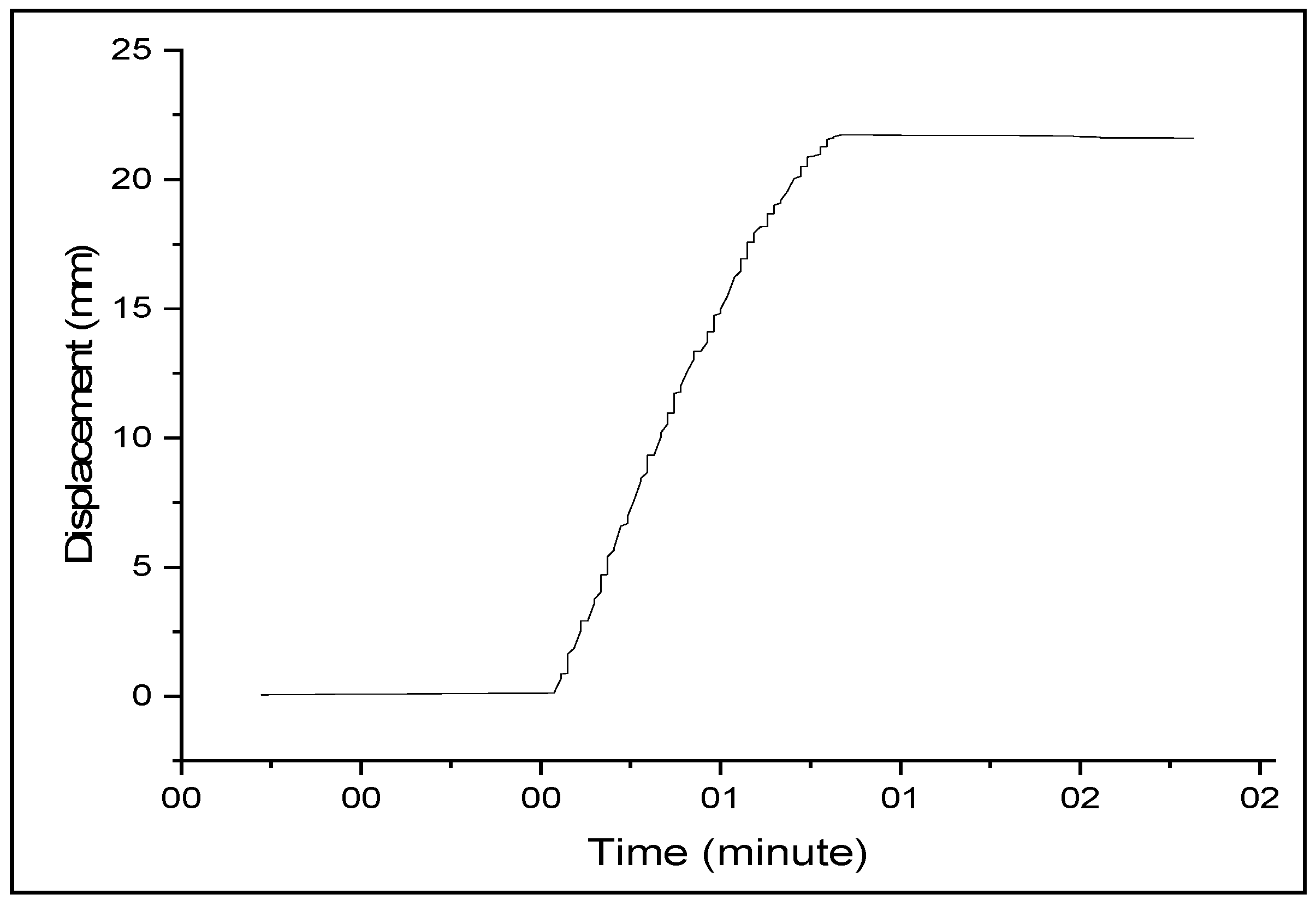
The self-developed large-scale direct shear setup was used to test the working behaviour of the developed sensor column for slope monitoring and failure prediction. Figure 18 shows the variation detected by the displacement induced using the hydraulic jack. A very small displacement was induced to check if the system could detect a small deviation in angle, and the displacement recorded through LVDT can be seen in Figure 19. In Figure 18, the maximum angle detected is only 0.5 degrees on the y-axis and 0.1 to 0.2 degrees on the x-axis. The system has some noise and variation in readings, but as it is very low limited to 0.01 to 0.05 degrees only thus can be ignored in further investigations or monitoring for better understanding.
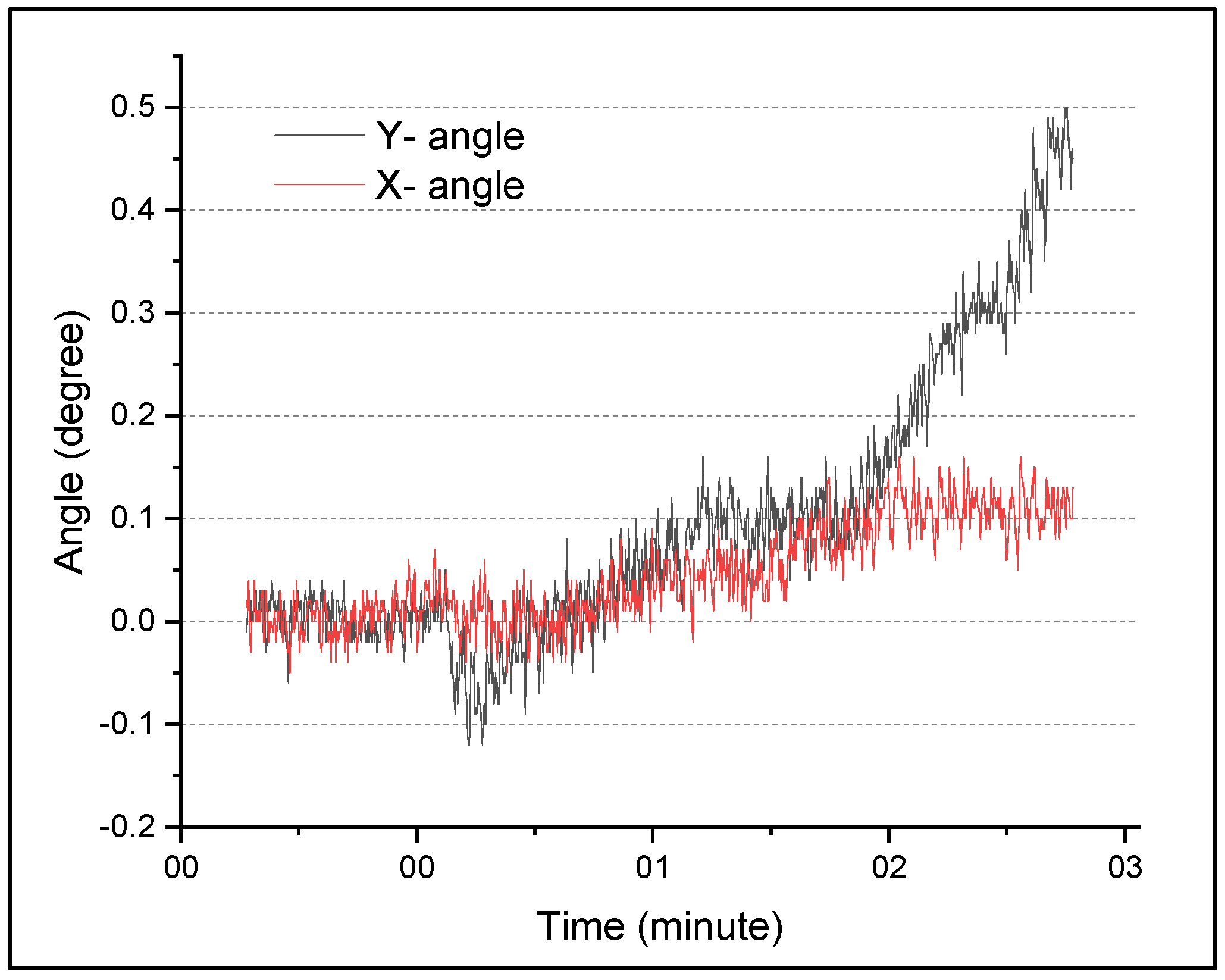
In further testing, the displacement was increased to a large extent to check the working of the sensor. There was a limitation to the LVDT sensor in that it could not measure such large deformation in this phase. Figure 20 shows the variation of angle when further displacement is introduced to the upper block. It shows that there is a large deviation detected in the y-axis as the slope usually moves downward against the y-axis. However, there is also some movement in the x-direction which can help in better monitoring of the slope.
5.2. Results of the Physical Model
A landslide that occurred in Kotrupi village was simulated in this study using the physical modelling method to study the failure mechanism under variable rainfall conditions. To monitor the movement of the slope, the self-developed tilt-based monitoring system was installed at the top section of the slope. The results generated from the tilt and soil moisture sensor were described in this section. A self-developed rainfall generator was used for the rainfall generation, and the input rainfall with respect to the cumulative rainfall depth is shown in this section which can be helpful in deciding the threshold rainfall for the particular slide or can be used to predict the threshold for the nearby areas.
5.2.1. Soil Properties
Dry and saturated unit weights were 16.7 kN/m3, and 20.3 kN/m3, respectively. The saturated permeability coefficient was 0.00023 m/sec, cohesion 21 kPa, and friction angle was 31°. This is because the soil in Kotrupi was mainly made up of very coarse sand as poorly graded sand (SP) in the USCS classification. The presence of moisture from the infiltration that the slope has experienced has resulted in the development of apparent cohesion. As a result, the apparent cohesiveness between different soil particles is revealed by the cohesion value that is achieved through triaxial testing. Additionally, the existence of fine soil, as measured by silt content (SM), has been of assistance in the development of the cohesion value. The liquid limit of slope material was found to be 32%. Extensive research has been done to investigate the geotechnical characterization of the Kotrupi landslide as it has been shown to vary in a wide range, although the results from this study fall in the region, which justifies the laboratory results [53,61,68,69].
5.2.2. Monitoring Results of Soil Slope
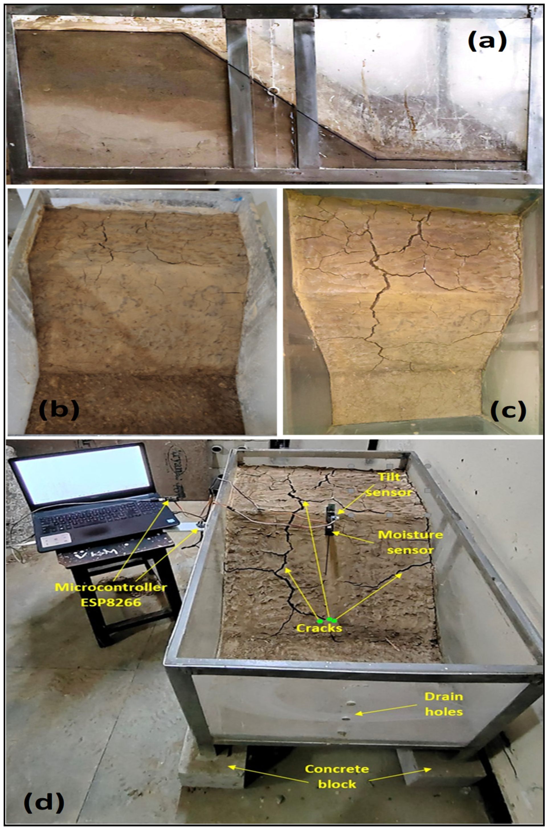
The physical slope model is prepared to study the effect of rainfall on the slope. To study the effect of pre-monsoonal rainfall, an antecedent rainfall of 10 mm was simulated at 1 mm/h intensity. Figure 21a shows that deep percolation takes place, which justifies that the low intensity and long duration rainfall causes deep saturation and may result in a deep-seated landslide. In Figure 21a, it can be seen that the slope is dry at the end, and the saturation level keeps increasing to the top. This may result in compaction and consolidation of soil near the junction point of wet and dry soil, which in turn decreases the permeability. Figure 21b shows the generation of small cracks on top of the slope takes place after one week. Figure 21c shows the effect after four weeks, and the wide cracks can be seen on top as well as the slope section that may be generated by soil shrinkage after wetting and drying. The duration of generated cracks may differ according to the temperature and humidity of the surrounding environment. Further rainfall on the slope results in faster and deeper percolation of water through the cracks, which helps in creating the fluidization zone between the dense and loose soil layer during the monsoonal season. The tilt sensors were mounted on top of a steel scale. At the bottom, a soil moisture sensor was attached and placed into the soil after creating a borehole using a drill machine (Figure 21d). Further, the sensors were installed on the upper section of the slope to monitor the slope movement and the water content.
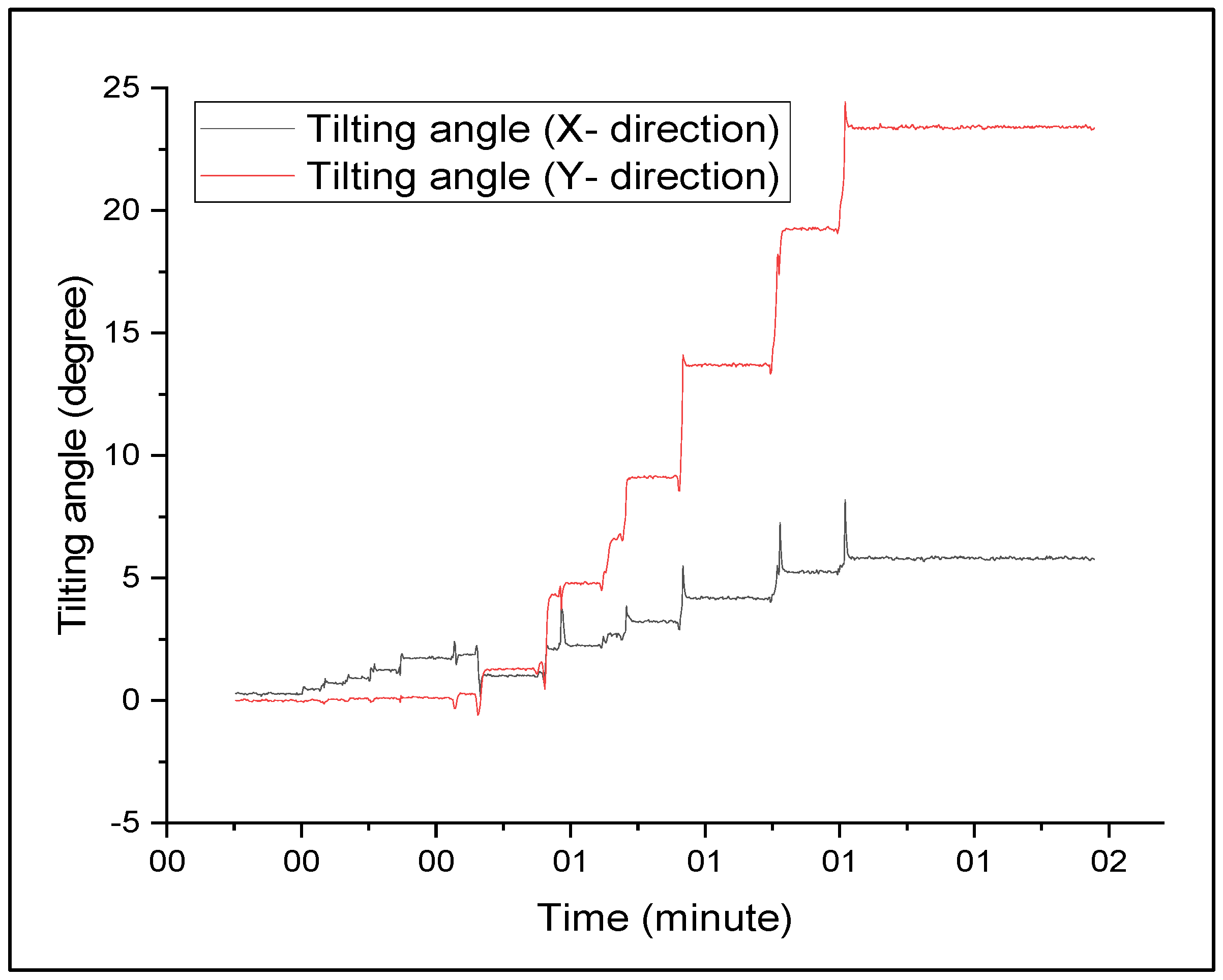
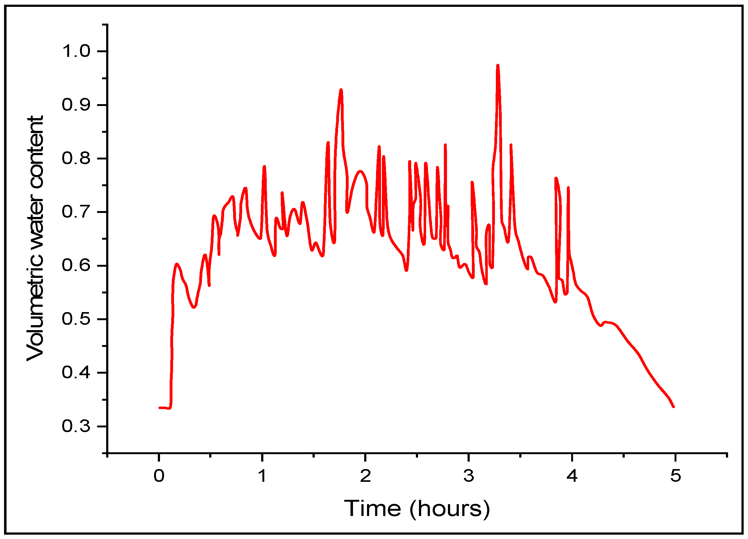
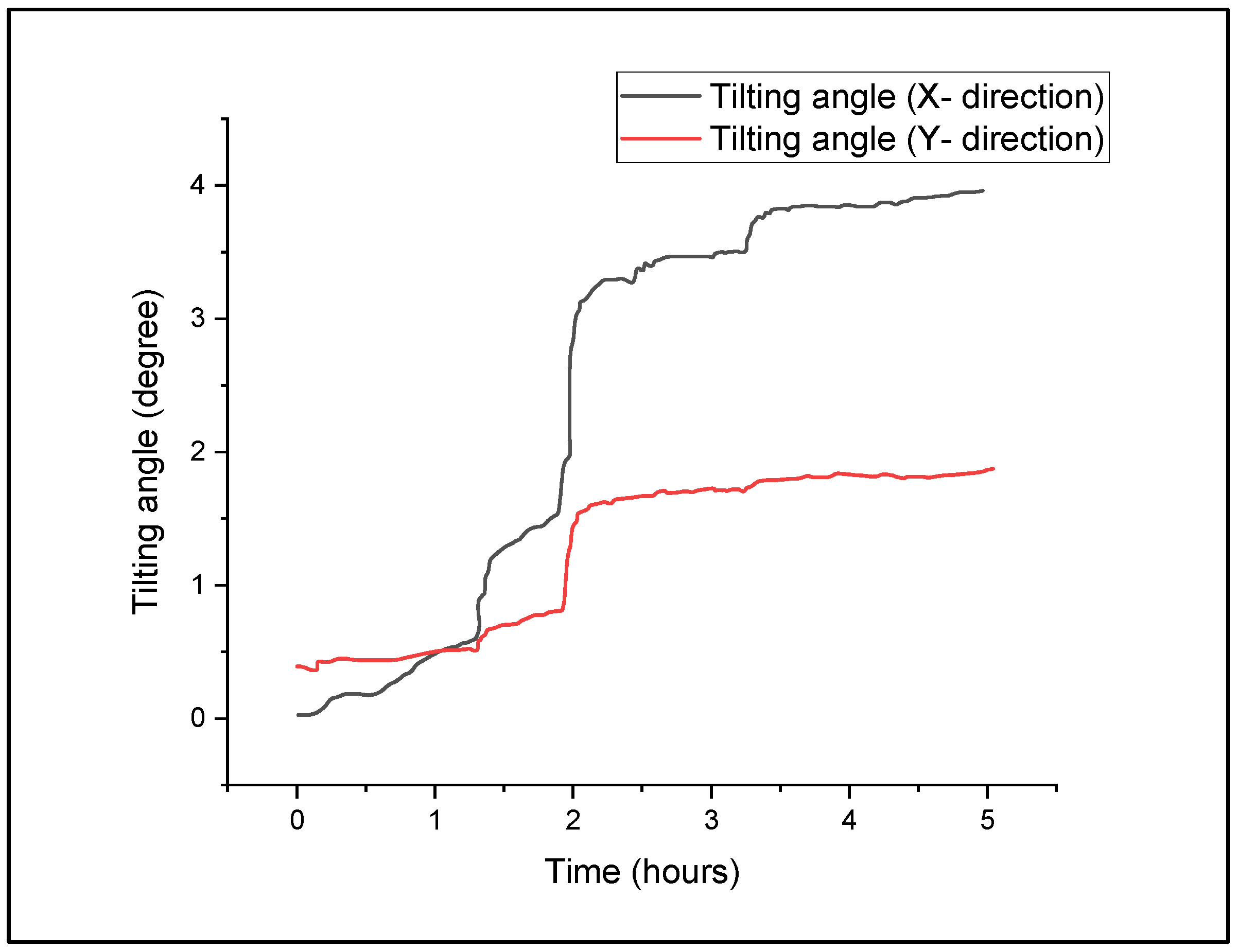
The rainfall was simulated by a self-developed rainfall generator equipped with a flow sensor and a microcontroller to record the flow. Figure 22 shows the variation of water content against the input rainfall. As the water content increases or varies according to the input rainfall, the water content change affects the slope stability; thus, the variation in the tilting angle can be seen in Figure 23. As the slope is much more likely to fail in the y-direction due to gravity action, the angle deviation is much more significant in the x-direction. There is also some deviation detected in the x-direction due to some rotation and settlement.
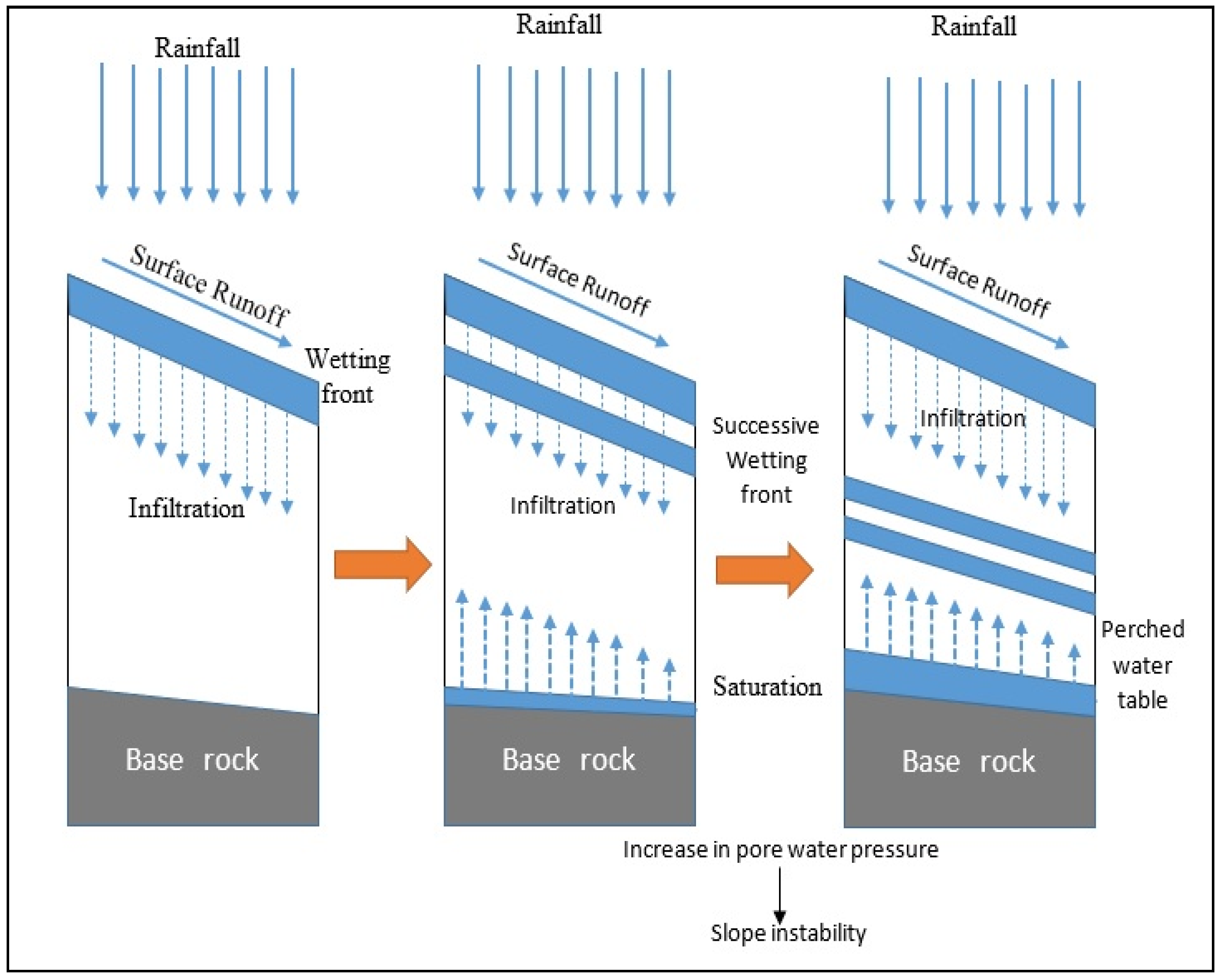
Many researchers worked around the globe in order to test the feasibility of tilt-based monitoring systems [42,44,70]. This study validates the effective monitoring of rainfall-induced landslides using a tilt sensor. A direct shear model setup was developed to verify the sensor’s working and prove its reliability [71]. The physical modelling method is used to simulate the soil slope to study the effect of pre and post-monsoonal rainfall on the slope and to test the monitoring sensor in a realistic environment [27,36]. Figure 21 also shows that wetting and drying can lead to the formation of cracks during pre-monsoonal rainfall, which can cause the water to infiltrate deep and may cause failure [30]. One study [43] stated that the change in water content is a better representation than just the water content and, as Figure 22 depicts, the variation in the volumetric water content is very vigorous, which may cause the slope to be unstable. Figure 23 also depicts the sudden variation in tilt angle during heavy rainfall, which validates the result. This study also proved the possible failure mechanism occurring in rainfall-induced landslides (Figure 24) [36,37].
6. Conclusions
The number of landslide incidents in the north Indian Himalayan region has increased dramatically in every monsoonal season. Mandi, a district in Himachal Pradesh, is among the widely affected areas. This research led to the following findings:
- A self-developed direct shear model was used to examine the effectiveness of a rudimentary monitoring system designed to prevent landslides caused by rainfall. Tilt sensors were placed on the slope’s surface in a physical slope model to detect any abnormal variation in the angle at which the sensors are tilted.
- The tilt and volumetric water content sensors were installed on the upper section of the slope and were confirmed with the displacement (Figure 20, Figure 21, Figure 22 and Figure 23). There was a sudden movement in slope recorded under the influence of applied rainfall in the course of the research. The precise amount of rain or rate of tilting required for landslides is hard to express.
- The findings show that prior rainfall causes slope displacement, supporting earlier research in this area. By adopting such a system, it may also be possible to validate existing rainfall threshold models produced, and the site-specific empirical equation can be created based on circumstances.
- The study proved that the cracks developed to cause deeper percolation, which leads to slope failure by generating the fluidization zone between the soil layer. Figure 24 explains the mechanism of landslide failure triggered by rainfall.
With timely data availability, this kind of attempt to put up an early warning system and validate the well-known empirical models would be enhanced, potentially saving lives by issuing an alarm for evacuation. This study can be further investigated with a numerical modelling method to analyse the rainfall-induced landslide and its validation so that numerical modelling can be used to analyse different slopes for prediction, as it is not possible to perform the physical model test for all slopes. Furthermore, automated warning systems can be added to the developed system to generate warnings in real-time. Although the developed system has only been evaluated for debris failure in this study, it could be evaluated in the future under varying geological conditions to assess its efficacy and feasibility in dealing with various types of landslides.
Author Contributions
A.P.P. has written the original draft, experiment, fabrication, analysis, validation, and figure preparation. A.K.S. has supervised the submitted work and provided the required resources. All authors have read and agreed to the published version of the manuscript.
Funding
This research received no external funding.
Institutional Review Board Statement
All authors have read, understood, and have complied as applicable with the statement on “Ethical responsibilities of Authors” as found in the Instructions for Authors.
Data Availability Statement
All data, models, or codes that support the findings of this study are available from the corresponding author upon reasonable request.
Acknowledgments
The authors are thankful to Delhi Technological University for providing the research facilities and funding to support this study.
Conflicts of Interest
The authors declare no conflict of interest.
References
- Parkash, S. Historical Records of Socio-Economically Significant Landslides in India. J. South Asia Disaster Stud. 2011, 4, 177–204. [Google Scholar]
- Guerriero, L.; Prinzi, E.P.; Calcaterra, D.; Ciarcia, S.; Di Martire, D.; Guadagno, F.M.; Ruzza, G.; Revellino, P. Kinematics and Geologic Control of the Deep-Seated Landslide Affecting the Historic Center of Buonalbergo, Southern Italy. Geomorphology 2021, 394, 107961. [Google Scholar] [CrossRef]
- Smith, D.M.; Oommen, T.; Bowman, L.J.; Gierke, J.S.; Vitton, S.J. Hazard Assessment of Rainfall-Induced Landslides: A Case Study of San Vicente Volcano in Central El Salvador. Nat. Hazards 2015, 75, 2291–2310. [Google Scholar] [CrossRef]
- Froude, M.J.; Petley, D.N. Global Fatal Landslide Occurrence from 2004 to 2016. Nat. Hazards Earth Syst. Sci. 2018, 18, 2161–2181. [Google Scholar] [CrossRef]
- Dikshit, A.; Sarkar, R.; Pradhan, B.; Segoni, S.; Alamri, A.M. Rainfall Induced Landslide Studies in Indian Himalayan Region: A Critical Review. Appl. Sci. 2020, 10, 2466. [Google Scholar] [CrossRef]
- Kanungo, D.P.; Sharma, S. Rainfall Thresholds for Prediction of Shallow Landslides around Chamoli-Joshimath Region, Garhwal Himalayas, India. Landslides 2014, 11, 629–638. [Google Scholar] [CrossRef]
- Can, E. Investigation of Landslide Potential Parameters on Zonguldak-Ereǧli Highway and Adverse Effects of Landslides in the Region. Environ. Monit. Assess. 2014, 186, 2435–2447. [Google Scholar] [CrossRef]
- Teja, T.S.; Dikshit, A.; Satyam, N. Determination of Rainfall Thresholds for Landslide Prediction Using an Algorithm-Based Approach: Case Study in the Darjeeling Himalayas, India. Geosciences 2019, 9, 302. [Google Scholar] [CrossRef]
- Dikshit, A.; Sarkar, R.; Satyam, N. Probabilistic Approach toward Darjeeling Himalayas Landslides-A Case Study. Cogent Eng. 2018, 5, 1537539. [Google Scholar] [CrossRef]
- Chen, Y.; Li, B.; Xu, Y.; Zhao, Y.; Xu, J. Field Study on the Soil Water Characteristics of Shallow Layers on Red Clay Slopes and Its Application in Stability Analysis. Arab. J. Sci. Eng. 2019, 44, 5107–5116. [Google Scholar] [CrossRef]
- Guzzetti, F.; Peruccacci, S.; Rossi, M.; Stark, C.P. The Rainfall Intensity-Duration Control of Shallow Landslides and Debris Flows: An Update. Landslides 2008, 5, 3–17. [Google Scholar] [CrossRef]
- Abraham, M.T.; Satyam, N.; Rosi, A.; Pradhan, B.; Segoni, S. The Selection of Rain Gauges and Rainfall Parameters in Estimating Intensity-Duration Thresholds for Landslide Occurrence: Case Study from Wayanad (India). Water 2020, 12, 1000. [Google Scholar] [CrossRef]
- Lari, S.; Frattini, P.; Crosta, G.B. A Probabilistic Approach for Landslide Hazard Analysis. Eng. Geol. 2014, 182, 3–14. [Google Scholar] [CrossRef]
- Glade, T.; Crozier, M.; Smith, P. Applying Probability Determination to Refine Landslide-Triggering Rainfall Thresholds Using an Empirical “Antecedent Daily Rainfall Model”. Pure Appl. Geophys. 2000, 157, 1059–1079. [Google Scholar] [CrossRef]
- Abraham, M.T.; Satyam, N.; Pradhan, B.; Alamri, A.M. Forecasting of Landslides Using Rainfall Severity and Soil Wetness: A Probabilistic Approach for Darjeeling Himalayas. Water 2020, 12, 804. [Google Scholar] [CrossRef]
- Tufano, R.; Cesarano, M.; Fusco, F.; Vita, P. De Probabilistic Approaches for Assessing Rainfall Thresholds Triggering Shallow Landslides. The Study Case of the Peri-Vesuvian Area (Southern Italy). Ital. J. Eng. Geol. Environ. 2019, 2019, 105–110. [Google Scholar] [CrossRef]
- Capparelli, G.; Tiranti, D. Application of the MoniFLaIR Early Warning System for Rainfall-Induced Landslides in Piedmont Region (Italy). Landslides 2010, 7, 401–410. [Google Scholar] [CrossRef]
- Dikshit, A.; Satyam, N. Application of FLaIR Model for Early Warning System in Chibo Pashyor, Kalimpong, India for Rainfall-Induced Landslides. Nat. Hazards Earth Syst. Sci. Discuss. 2017, 295. [Google Scholar] [CrossRef]
- Panchal, S.; Shrivastava, A.K. A Comparative Study of Frequency Ratio, Shannon’s Entropy and Analytic Hierarchy Process (Ahp) Models for Landslide Susceptibility Assessment. ISPRS Int. J. Geo-Inf. 2021, 10, 603. [Google Scholar] [CrossRef]
- Das, S.; Sarkar, S.; Kanungo, D.P. GIS-Based Landslide Susceptibility Zonation Mapping Using the Analytic Hierarchy Process (AHP) Method in Parts of Kalimpong Region of Darjeeling Himalaya. Environ. Monit. Assess. 2022, 194, 234. [Google Scholar] [CrossRef]
- Ibrahim, M.B.; Mustaffa, Z.; Balogun, A.B.; Indra, S.H.H.; Nur Ain, A. Landslide’s Analysis and Hazard Mapping Based on ANALYTIC HIERARCHY PROCESS (AHP) Using GIS, in Lawas, Sabah-Sarawak. IOP Conf. Ser. Earth Environ. Sci. 2022, 1064, 012031. [Google Scholar] [CrossRef]
- Selamat, S.N.; Majid, N.A.; Taha, M.R.; Osman, A. Application of Geographical Information System (GIS) Using Artificial Neural Networks (ANN) for Landslide Study in Langat Basin, Selangor. IOP Conf. Ser. Earth Environ. Sci. 2022, 1064, 012052. [Google Scholar] [CrossRef]
- Pradhan, B.; Al-Najjar, H.A.H.; Sameen, M.I.; Mezaal, M.R.; Alamri, A.M. Landslide Detection Using a Saliency Feature Enhancement Technique from LiDAR-Derived DEM and Orthophotos. IEEE Access 2020, 8, 121942–121954. [Google Scholar] [CrossRef]
- Singh, N.; Gupta, S.K.; Shukla, D.P. Analysis of Landslide Reactivation Using Satellite Data: A Case Study of Kotrupi Landslide, Mandi, Himachal Pradesh, India. Int. Arch. Photogramm. Remote Sens. Spat. Inf. Sci. 2020, 42, 137–142. [Google Scholar] [CrossRef]
- Tiwari, B.; Ajmera, B. Physical Modelling of Rain-Induced Landslides. In Landslide Dynamics: ISDR-ICL Landslide Interactive Teaching Tools; Springer: Cham, Switzerland, 2018; pp. 277–285. [Google Scholar]
- Matziaris, V.; Marshall, A.M.; Heron, C.M.; Yu, H.S. Centrifuge Model Study of Thresholds for Rainfall-Induced Landslides in Sandy Slopes. IOP Conf. Ser. Earth Environ. Sci. 2015, 26, 012032. [Google Scholar] [CrossRef]
- Li, C.; Yao, D.; Wang, Z.; Liu, C.; Wuliji, N.; Yang, L.; Li, L.; Amini, F. Model Test on Rainfall-Induced Loess–Mudstone Interfacial Landslides in Qingshuihe, China. Environ. Earth Sci. 2016, 75, 835. [Google Scholar] [CrossRef]
- Huang, X.; Dong, Y. Study on Physical and Mechanical Properties of Soil in a Loess Landslide. J. Phys. Conf. Ser. 2023, 2424, 012010. [Google Scholar] [CrossRef]
- Rahardjo, H.; Ong, T.H.; Rezaur, R.B.; Leong, E.C. Factors Controlling Instability of Homogeneous Soil Slopes under Rainfall. J. Geotech. Geoenviron. Eng. 2007, 133, 1532–1543. [Google Scholar] [CrossRef]
- Acharya, K.P.; Bhandary, N.P.; Dahal, R.K.; Yatabe, R. Seepage and Slope Stability Modelling of Rainfall-Induced Slope Failures in Topographic Hollows. Geomat. Nat. Hazards Risk 2016, 7, 721–746. [Google Scholar] [CrossRef]
- Singh, A.K.; Kundu, J.; Sarkar, K. Stability Analysis of a Recurring Soil Slope Failure along NH-5, Himachal Himalaya, India. Nat. Hazards 2018, 90, 863–885. [Google Scholar] [CrossRef]
- Paswan, A.P.; Shrivastava, A.K. Stability Analysis of Rainfall-Induced Landslide. In Proceedings of the 3rd International Online Conference on Emerging Trends in Multi-Disciplinary Research “ETMDR-2022”, Jaipur, Rajasthan, India, 20–22 January 2022; pp. 505–509. [Google Scholar]
- Paswan, A.P.; Shrivastava, A.K. Numerical Modelling of Rainfall-Induced Landslide. In Proceedings of the International e-Conference on Sustainable Development & Recent Trends in Civil Engineering, New Delhi, India, 4–5 January 2022; pp. 8–13. [Google Scholar]
- Jing, F.; Ling, H.S.; Xiuli, D.; Jinlong, W. Influence of Rainfall on Transient Seepage Field of Deep Landslides: A Case Study of Area II of Jinpingzi Landslide. IOP Conf. Ser. Earth Environ. Sci. 2020, 570, 022056. [Google Scholar] [CrossRef]
- Tufano, R.; Formetta, G.; Calcaterra, D.; De Vita, P. Hydrological Control of Soil Thickness Spatial Variability on the Initiation of Rainfall-Induced Shallow Landslides Using a Three-Dimensional Model. Landslides 2021, 18, 3367–3380. [Google Scholar] [CrossRef]
- Paswan, A.P.; Shrivastava, A.K. Modelling of Rainfall - Induced Landslide: A Threshold-Based Approach. Arab. J. Geosci. 2022, 15, 795. [Google Scholar] [CrossRef]
- Dahal, R.K.; Hasegawa, S.; Nonomura, A.; Yamanaka, M.; Masuda, T.; Nishino, K. Failure Characteristics of Rainfall-Induced Shallow Landslides in Granitic Terrains of Shikoku Island of Japan. Environ. Geol. 2009, 56, 1295–1310. [Google Scholar] [CrossRef]
- Intrieri, E.; Gigli, G.; Mugnai, F.; Fanti, R.; Casagli, N. Design and Implementation of a Landslide Early Warning System. Eng. Geol. 2012, 147–148, 124–136. [Google Scholar] [CrossRef]
- Zhi, M.; Shang, Y.; Zhao, Y.; Lü, Q.; Sun, H. Investigation and Monitoring on a Rainfall-Induced Deep-Seated Landslide. Arab. J. Geosci. 2016, 9, 182. [Google Scholar] [CrossRef]
- Kanungo, D.P.; Maletha, A.K.; Singh, M. Ground Based Wireless Instrumentation and Real Time Monitoring of Pakhi Landslide, Garhwal Himalayas, Uttarakhand (India). In Advancing Culture of Living with Landslides; Springer: Cham, Switzerland, 2017. [Google Scholar] [CrossRef]
- Guerriero, L.; Guerriero, G.; Grelle, G.; Guadagno, F.M.; Revellino, P. Brief Communication: A Low-Cost Arduino®-Based Wire Extensometer for Earth Flow Monitoring. Nat. Hazards Earth Syst. Sci. 2017, 17, 881–885. [Google Scholar] [CrossRef]
- Abraham, M.T.; Satyam, N.; Pradhan, B.; Alamri, A.M. Iot-Based Geotechnical Monitoring of Unstable Slopes for Landslide Early Warning in the Darjeeling Himalayas. Sensors 2020, 20, 2611. [Google Scholar] [CrossRef] [PubMed]
- Uchimura, T.; Towhata, I.; Anh, T.T.L.; Fukuda, J.; Bautista, C.J.B.; Wang, L.; Seko, I.; Uchida, T.; Matsuoka, A.; Ito, Y.; et al. Simple Monitoring Method for Precaution of Landslides Watching Tilting and Water Contents on Slopes Surface. Landslides 2010, 7, 351–357. [Google Scholar] [CrossRef]
- Qiao, S.; Feng, C.; Yu, P.; Tan, J.; Uchimura, T.; Wang, L.; Tang, J.; Shen, Q.; Xie, J. Investigation on Surface Tilting in the Failure Process of Shallow Landslides. Sensors 2020, 20, 2662. [Google Scholar] [CrossRef]
- Artese, G.; Perrelli, M.; Artese, S.; Meduri, S.; Brogno, N. POIS, a Low Cost Tilt and Position Sensor: Design and First Tests. Sensors 2015, 15, 10806–10824. [Google Scholar] [CrossRef]
- Dikshit, A.; Satyam, D.N.; Towhata, I. Early Warning System Using Tilt Sensors in Chibo, Kalimpong, Darjeeling Himalayas, India. Nat. Hazards 2018, 94, 727–741. [Google Scholar] [CrossRef]
- Dahal, R.K. Rainfall-Induced Landslides in Nepal. Int. J. Eros. Control Eng. 2012, 5, 1–8. [Google Scholar] [CrossRef]
- Kelleners, T.J.; Soppe, R.W.O.; Robinson, D.A.; Schaap, M.G.; Ayars, J.E.; Skaggs, T.H. Calibration of Capacitance Probe Sensors Using Electric Circuit Theory. Soil Sci. Soc. Am. J. 2004, 68, 430–439. [Google Scholar] [CrossRef]
- Placidi, P.; Gasperini, L.; Grassi, A.; Cecconi, M.; Scorzoni, A. Characterization of Low-Cost Capacitive Soil Moisture Sensors for IoT Networks. Sensors 2020, 20, 3585. [Google Scholar] [CrossRef]
- Hrisko, J. Capacitive Soil Moisture Sensor Calibration with Arduino; Maker Portal LLC: New York, NY, USA, 2020; pp. 1–24. [Google Scholar]
- Ida, N. Engineering Electromagnetics; Springer: Cham, Switzerland, 2015; ISBN 9783319078052. [Google Scholar]
- DFROBOT Capacitive Soil Moisture Sensor SKU:SEN0193 v.2.0. Available online: https://wiki.dfrobot.com/Capacitive_Soil_Moisture_Sensor_SKU_SEN0193 (accessed on 21 November 2022).
- Ilamkar, P.T.; Kohli, A. Report on Geological Assessment of Kotrupi Landslide, Mandi—Jogindernagar—Pathankot National Highway (N.H.-154), Tehsil Padhar, District Mandi, Himachal Pradesh. Geol. Surv. India 2017, 6, 5–9. [Google Scholar]
- ISRO Kotrupi Landslide, Mandi District, Himachal Pradesh, A Preliminary Report; National Remote Sensing Centre/ISRO: Hyderabad, India, 2017; Volume 2, pp. 4–6.
- Prakash, S.; Kathait, A. A Case Study on Kotrupi Landslide 2017, Mandi District, Himachal Pradesh National; National Institute of Disaster Management (NIDM), Ministry of Home Affairs, Government of India: New Delhi, India, 2021; ISBN 9789382571612. [Google Scholar]
- QGIS Development Team. QGIS Desktop 3.16 User Guide; Free Software Foundation: Boston, MA, USA, 2021; p. 1335. Available online: https://docs.qgis.org/3.16/pdf/en/QGIS-3.16-DesktopUserGuide-en.pdf (accessed on 21 November 2022).
- IS:2720 (Part 4); Methods of Test for Soils, Part 4: Grain Size Analysis. Bureau of Indian Standard: New Delhi, India, 1985; pp. 1–38.
- GEO-SLOPE International Ltd. Seepage Modeling with SEEP/W 2015; Geostudio Help—GEO-SLOPE International Ltd.: Calgary, AB, Canada, 2012; p. 199. [Google Scholar]
- IS: 2720 (Part 5); Determination of Liquid and Plastic Limit. Bureau of Indian Standard: New Delhi, India, 1985; pp. 1–16.
- IS: 2720 (Part 7-1980); Determination of Water Content-Dry Density Relation Using Light Compaction. Bureau of Indian Standard: New Delhi, India, 2011; pp. 1–16.
- Sharma, P.; Rawat, S.; Gupta, A.K. Study and Remedy of Kotropi Landslide in Himachal Pradesh, India. Indian Geotech. J. 2019, 49, 603–619. [Google Scholar] [CrossRef]
- Anderson, S.A.; Sitar, N. Analysis of Rainfall-Induced Debris Flows. J. Geotech. Eng. 1995, 121, 544–552. [Google Scholar] [CrossRef]
- IS: 2720 (Part 11); Determination of the Shear Strength Parameters of a Specimen Tested in Unconsolidated Undrained Triaxial Compression without the Measurement of Pore Water Pressure. Bureau of Indian Standard: New Delhi, India, 1993.
- Askarinejad, A.; Laue, J.; Zweidler, A.; Iten, M.; Bleiker, E.; Buschor, H.; Springman, S.M. Physical Modelling of Rainfall Induced Landslides under Controlled Climatic Conditions. In Proceedings of the Eurofuge 2012, 2nd Eurofuge Conference on Physical Modelling in Geotechnics, Deltares, Delft, The Netherlands, 23–24 April 2012. [Google Scholar]
- Luo, Y.; He, S.M.; Chen, F.Z.; Li, X.P.; He, J.C. A Physical Model Considered the Effect of Overland Water Flow on Rainfall-Induced Shallow Landslides. Geoenviron. Disasters 2015, 2, 8. [Google Scholar] [CrossRef]
- Iverson, R.M. Landslide Triggering by Rain Infiltration. Water Resour. Res. 2000, 36, 1897–1910. [Google Scholar] [CrossRef]
- Godt, J.W.; Baum, R.L.; Lu, N. Landsliding in Partially Saturated Materials. Geophys. Res. Lett. 2009, 36, L02403. [Google Scholar] [CrossRef]
- Pradhan, S.P.; Panda, S.D.; Roul, A.R.; Thakur, M. Insights into the Recent Kotropi Landslide of August 2017, India: A Geological Investigation and Slope Stability Analysis. Landslides 2019, 16, 1529–1537. [Google Scholar] [CrossRef]
- Mali, N.; Shukla, D.P.; Kala, V.U. Identifying Geotechnical Characteristics for Landslide Hazard Indication: A Case Study in Mandi, Himachal Pradesh, India. Arab. J. Geosci. 2022, 15, 144. [Google Scholar] [CrossRef]
- Uchimura, T.; Towhata, I.; Wang, L.; Nishie, S.; Yamaguchi, H.; Seko, I.; Qiao, J. Precaution and Early Warning of Surface Failure of Slopes Using Tilt Sensors. Soils Found. 2015, 55, 1086–1099. [Google Scholar] [CrossRef]
- Dixon, N.; Smith, A.; Flint, J.A.; Khanna, R.; Clark, B.; Andjelkovic, M. An Acoustic Emission Landslide Early Warning System for Communities in Low-Income and Middle-Income Countries. Landslides 2018, 15, 1631–1644. [Google Scholar] [CrossRef]
Figure 1.
Landslide hazard in Himachal Pradesh (Source: HPSDMA).

Figure 2.
Design of the low-cost framework for monitoring landslides.

Figure 3.
MPU6050 module (a) sensor module, (b) working axis details, and (c) circuit diagram.

Figure 4.
Block diagram of MPU6050 Module.

Figure 5.
Parallel plate capacitor setup.

Figure 6.
Illustration concept behind working of soil moisture sensor.

Figure 7.
A capacitive soil moisture sensor v2.0.

Figure 8.
Circuit diagram of the capacitive sensors (source: Sensor DFROBOT data sheet).

Figure 9.
A map showing the location of the research area.

Figure 10.
Satellite view of the study area.

Figure 11.
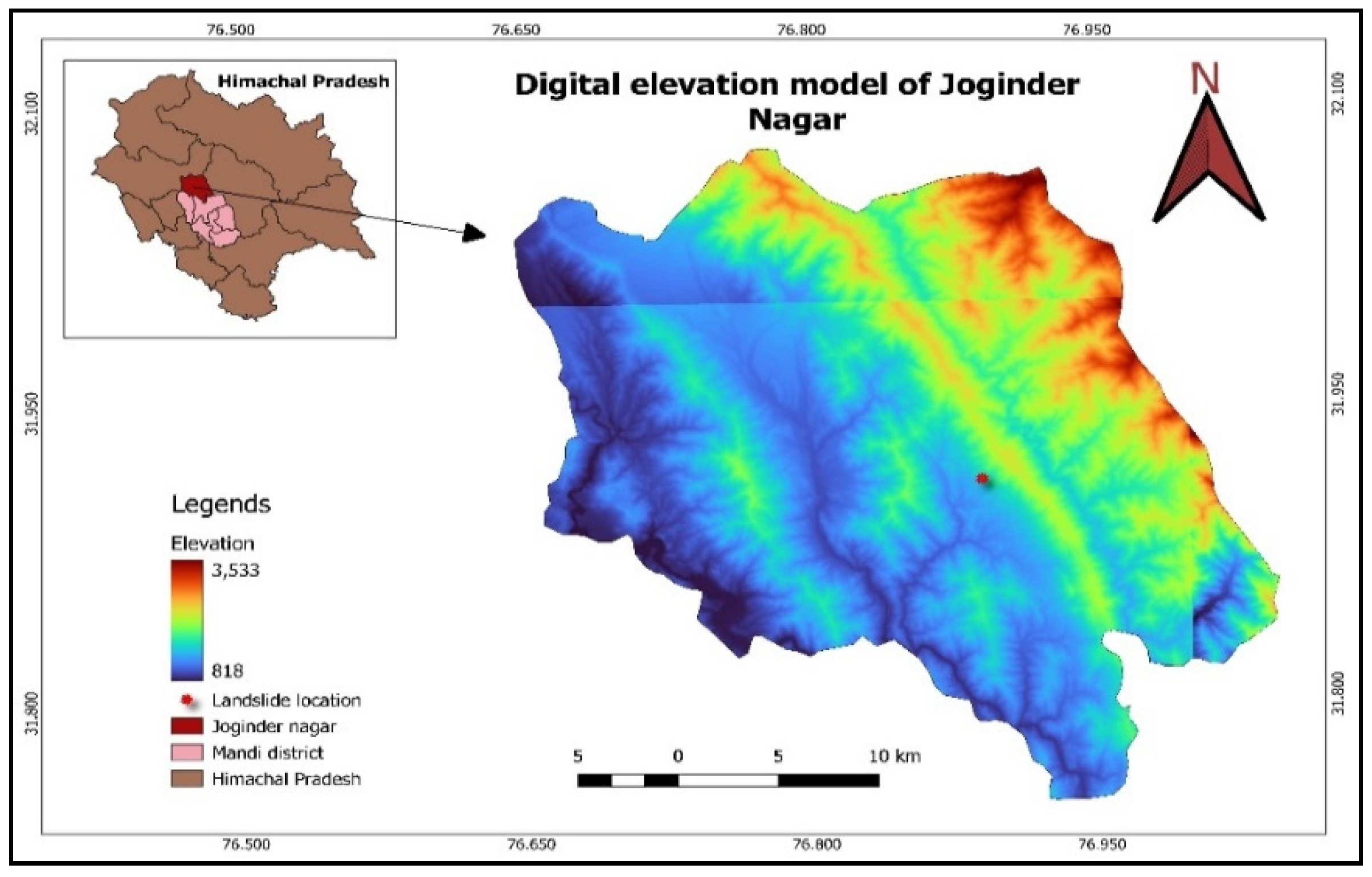
SRTM-DEM of Joginder Nagar, Mandi, Himachal Pradesh.

Figure 12.
Flow chart of the methodology adopted in the study.

Figure 13.
The schematic diagram depicts a large-scale physical model of a slope failure used to accelerate the top box relative to the bottom to analyse the displacement behaviour with tilt measurements.
Figure 13.
The schematic diagram depicts a large-scale physical model of a slope failure used to accelerate the top box relative to the bottom to analyse the displacement behaviour with tilt measurements.

Figure 14.
Modelling and casting of blocks with boreholes of 4 cm.

Figure 15.
Self-developed large-scale direct shear setup.

Figure 16.
Schematic diagram of experimental setup.

Figure 17.
Input Rainfall parameter.

Figure 18.
Variation of angle in X and Y direction.

Figure 19.
Linear displacement in X direction using LVDT.

Figure 20.
Variation of angle in X and Y direction.

Figure 21.
Physical model setup (a) percolation of water, (b) visible small cracks, (c) formation of larger cracks, and (d) placement of sensors.
Figure 21.
Physical model setup (a) percolation of water, (b) visible small cracks, (c) formation of larger cracks, and (d) placement of sensors.

Figure 22.
Output volumetric water content.

Figure 23.
Variation of angle in X and Y direction.

Figure 24.
Sequential schematic of landslide initiation.

Disclaimer/Publisher’s Note: The statements, opinions and data contained in all publications are solely those of the individual author(s) and contributor(s) and not of MDPI and/or the editor(s). MDPI and/or the editor(s) disclaim responsibility for any injury to people or property resulting from any ideas, methods, instructions or products referred to in the content. |
© 2023 by the authors. Licensee MDPI, Basel, Switzerland. This article is an open access article distributed under the terms and conditions of the Creative Commons Attribution (CC BY) license (https://creativecommons.org/licenses/by/4.0/).
Share and Cite
MDPI and ACS Style
Paswan, A.P.; Shrivastava, A.K. Evaluation of a Tilt-Based Monitoring System for Rainfall-Induced Landslides: Development and Physical Modelling. Water 2023, 15, 1862. https://doi.org/10.3390/w15101862
AMA Style
Paswan AP, Shrivastava AK. Evaluation of a Tilt-Based Monitoring System for Rainfall-Induced Landslides: Development and Physical Modelling. Water. 2023; 15(10):1862. https://doi.org/10.3390/w15101862
Chicago/Turabian StylePaswan, Abhishek Prakash, and Amit Kumar Shrivastava. 2023. "Evaluation of a Tilt-Based Monitoring System for Rainfall-Induced Landslides: Development and Physical Modelling" Water 15, no. 10: 1862. https://doi.org/10.3390/w15101862
Note that from the first issue of 2016, this journal uses article numbers instead of page numbers. See further details here.