Water Quality Index Estimations Using Machine Learning Algorithms: A Case Study of Yazd-Ardakan Plain, Iran

Abstract

Excessive population growth and high water demands have significantly increased water extractions from deep and semi-deep wells in the arid regions of Iran. This has negatively affected water quality in different areas. The Water Quality Index (WQI) is a suitable tool to assess such impacts. This study used WQI and the fuzzy hierarchical analysis process of the water quality index (FAHP-WQI) to investigate the water quality status of 96 deep agricultural wells in the Yazd-Ardakan Plain, Iran. Calculating the WQI is time-consuming, but estimating WQI is inevitable for water resources management. For this purpose, three Machine Learning (ML) algorithms, namely, Gene Expression Programming (GEP), M5P Model tree, and Multivariate Adaptive Regression Splines (MARS), were employed to predict WQI. Using Wilcox and Schoeller charts, water quality was also investigated for agricultural and drinking purposes. The results demonstrated that 75% and 33% of the study area have good quality, based on the WQI and FAHP-WQI methods, respectively. According to the results of the Wilcox chart, around 37.25% of the wells are in the C3S2 and C3S1 classes, which indicate poor water quality. Schoeller’s diagram placed the drinking water quality of the Yazd-Ardakan plain in acceptable, inadequate, and inappropriate categories. Afterwards, WQI, predicted by means of ML models, were compared on several statistical criteria. Finally, the comparative analysis revealed that MARS is slightly more accurate than the M5P model for estimating WQI.

1. Introduction

Water plays a vital role in agriculture and food production in many arid and semi-arid regions of Iran. A large number of studies in the field of water resources have been devoted to addressing the issues related to limited water resources, climate change, drought, groundwater discharge, and declining quality of surface water and groundwater in Iran [1,2,3]. Water supply issues in developing countries is not merely due to the scarcity of water resources, but also because of the lack of appropriate technologies for water supply, improper treatment and distribution network, insufficient use of national or international financial resources, and lack of implementation of necessary strategies in accordance with national, regional, and local conditions. Considering groundwater pollution in Iran, which has become a challenge in the past years, it is necessary to adopt a practical and adequate drinking water quality assessment framework for decision making. The water quality index (WQI), first proposed by Horton [4], is widely used to classify quality of surface water and groundwater. In this method, the most important parameters are first selected by professional experts, and then, the indices with the highest quality are calculated, based on the standard value or the expected limit for each parameter. A proper weight is then assigned to each parameter, relative to its impact on health or other aspects of concern. Finally, water quality is interpreted as values in the range of good to bad [5]. The lower the WQI values, the better the water quality conditions.

The Wilcox method is used in agriculture to classify water quality [6]. In this classification method, two parameters of EC and SAR are used. The value of EC correlates with salinity and determines the risk of sodium in terms of SAR [6]. Studies have also been conducted on the quality of drinking water. Healthy drinking water must have good quality indicators (including physical and chemical characteristics). The World Health Organization (WHO), the Ministry of Energy, and the Iranian Institute of Standards and Industrial Research, have provided standards for soluble salts and different pollutants in drinking water [7,8]. One of the methods to evaluate water quality in terms of drinkability is to use the Schoeller diagram. This diagram shows the relevant concentration of different parameters and enables a comparison [9,10,11]. Over the past two decades, fuzzy logic has been commonly used in most research fields and readily accepted by researchers and decision makers. The idea of fuzzy logic was propounded in Ref. [12]. It is especially popular in earth sciences, water resources and water quality management due to its capability in controlling uncertainties Thus, much attention has been granted to the development of environmental indicators using fuzzy logic [13].

Water quality assessment includes collecting samples, testing in the laboratory, and applying data, which are mainly long, time-consuming and expensive processes. In some countries, there is no opportunity to take samples and conduct tests due to poor economic conditions. Therefore, using a cost-effective tool to evaluate water quality faster and more accurately would be very useful. In this regard, artificial intelligence (AI) models are a suitable alternative to reduce costs and save time and can significantly help. Artificial intelligence technology is a powerful and potentially multifunctional tool in water science-related fields [14].

The concept of the water quality index is relatively new, and, in the last few decades, many researchers have utilized the WQI method worldwide. Furthermore, many studies have been conducted to predict WQI by evaluating the performance of different artificial intelligence models. Palani, et al. [15] used an artificial neural network model to predict and evaluate temperature, salinity, DO, and Chl-a in the Johor River on the coast of Singapore. In this research, artificial neural network models were used to predict the quantitative properties of water. The simulation accuracy measured in Nash—Sutcliffe ranged from 0.8 to 0.9 for training and testing data. Bashi-Azghadi, et al. [16] identified a source of contamination in a groundwater resource system using PSVM and PNN. The amount of leakage was estimated through the observed concentration of the quality index. It was concluded that the proposed methods were very effective in determining the source of pollution. Lumb, et al. [17], conducted a comprehensive review study on the emergence and evolution of the water quality index over the years, and proposed directions for future studies. They also outlined the major limitations of the index development process and made recommendations to overcome the problems. Gazzaz, et al. [18], in a study on the Kinta River in Malaysia, showed that ANN has an excellent ability to predict the WQI value, and the accuracy value of the model in this study was 0.97, which indicated high accuracy of the model. Boateng, et al. [19] collected and analyzed a total of 19 groundwater samples. In this study, the groundwater quality index showed that most of the samples were in the category of good to excellent, which indicated the suitability of groundwater for drinking and other household use. Adimalla and Qian [20] conducted a study in South India and investigated the water quality index for drinking purposes. Residents of this area use underground water to supply their water needs, so the importance of this source is very high. The results found that the nitrate concentration in more than 61% of the prepared samples was higher than the permissible limits. WQI values showed that 86% of the studied area had low water quality for drinking purposes. The health risk was also investigated, and it was found that excessive consumption of nitrate-contaminated groundwater has a higher health risk for infants than children and adults in this area. Brahim, et al. [21], in a study in the Kebilli region, investigated groundwater quality using the water quality index and fuzzy logic. The values of the WQI index for drinking and irrigation water were between 421.83 to 436.858 and 50 to 77, respectively. The correlation of fuzzy membership levels showed high values, between 0.88 and 0.79, for drinking and irrigation purposes, respectively. Kouadri et al. [14] used eight artificial intelligence algorithms to generate WQI forecasts in the Illizi region, southeastern Algeria. Two different scenarios were used to check the accuracy of the models when compared to one another. The results showed that the MLR and RF models were more accurate in the first and second scenarios, respectively, than other models. In another study, Khoi et al. [22] evaluated the performance of twelve machine learning (ML) models in surface water quality estimation in the Labung River in Vietnam. Water quality data from 2010 to 2017 were used to calculate the water quality index (WQI). The performance of each machine learning model was evaluated using R2 and RMSE. The results showed that all the models performed well, but the extreme gradient boosting (XGBoost) performed best, with the highest accuracy.

After a complete review of the previous literature, as far as the author knows, no research has been conducted (especially in the Yazd-Ardakan plain, Iran) that, in addition to investigating the water quality index, and predicting it with three artificial intelligence models, namely, Gene Expression Programming, M5P Model tree, and Multivariate Adaptive Regression Splines, compares performance in groundwater prediction. Such a study is important to the analysis of water quality. However, taking water quality samples is challenging, due to the costly and time-consuming techniques required to check the quality of water.

The current research aimed to determine groundwater quality in the Yazd-Ardakan region in the Yazd province to gain a proper perspective, and understanding, of the water quality resources. Due to the time-consuming calculation of the water quality index, machine learning algorithms were used to estimate WQI. Finally, the results of each of the algorithms were compared with one another so that the best one was selected to estimate the value of the water quality index. In the meantime, Wilcox and Schoeller’s charts were used to examine water quality for agricultural and drinking purposes.

2. Materials and Methods

2.1. Study Area

The Yazd-Ardakan Plain was selected as the study area. The plain, which covers an area of 8050 square kilometers, is part of the Siah Kooh basin and is approximately located in the center of Yazd province, Iran. (Longitude from 53°46′ to 55° and latitude from 31°49′ to 32°55′). The plain is bounded by the Siah Kooh desert in the north, and the Shir Kooh heights ridge in the south. Shirkooh is the highest point of the basin, with an elevation of 4037 m above the mean sea level, and the lowest point, which lies at the edge of the Siah Kooh desert, has an elevation of 970. The average height of the basin is 1565 m. Figure 1 shows the study area with sampling points.

The study area is in the sedimentary structural unit, and inherits some tectonic, stratigraphic, magmatic and metamorphic features of central Iran. The geology of the region mostly dates to the Quaternary era [23]. The evaporation rate in the city of Yazd is above 3000 mm per year, and the average temperature in the city is 18.9 degrees Celsius, while the average relative humidity is equal to 35.3%. Groundwater resources are depleted due to extraction from wells, aqueducts, and springs. The total annual depletion of ground water resources is about 617 million cubic meters, 92% of which is used in agriculture, 5% for drinking and health, and the remaining portion for use in industry and for livestock [23]. The groundwater generally flows from southwest to northeast.

2.2. Water Quality Index

The WQI is used to assess groundwater quality and for various purposes, such as drinking and irrigation. WQI has been used by various researchers in different parts of the world [24,25,26]. Water quality index, as per the World Health Organization (WHO) requirements, was calculated using the permissible limits for the parameters listed in

Table 1. Permissible limit for each parameter [23].

Chemical Parameters	K+	Na+	pH	Ca2+	${\mathrm{SO}}_4^{2-}$	Cl−	${\mathrm{HCO}}_3^{-}$	EC	TH	TDS	Mg2+
Sn	12	200	8.5	200	250	600	120	1500	500	1500	150

.

Water quality grades are calculated using the Equation (1) [23]:

$$q_n=100\left(\frac{V_n-V_i}{S_n-V_i}\right)$$

(1)

where, $q_n$ is water quality grading for parameter n, $V_i$ represents the ideal value for the parameter n, $V_n$ is the Observed value of the parameter n and $S_n$ is the standard permissible value for the parameter n.

The unit weight of the corresponding parameter n ($W_n)$, is defined as the inverse of the recommended standard value, $S_n$:

$$W_n=K/S_n$$

(2)

where $W_n$ is the weight unit of the parameter n, K denotes the standard value of the parameter n, while $S_n$ represents a proportionality constant.

The proportionality constant is also calculated using Equation (3):

$$k=1/\sum (1/S_n)$$

(3)

The total water quality index is then calculated linearly by adding the quality grade to the unit weight.

$$\mathrm{WQI}=\sum q_n{W}_n /\sum W_n$$

(4)

As shown in

Table 2. Water quality classification based on WQI definition [25].

Class	WQI Value	Water Quality Status
A	<50	Excellent
B	51–100	Good
C	101–200	Poor Water
D	201–300	Very Poor Water
E	>300	Water Unsuitable for Drinking

, the calculated values of the water quality index are usually classified into 5 classes: excellent, good, poor, very poor and unsuitable.

In addition to evaluation of measured chemical parameters, the parameters and indicators of salinity and alkalinity risks were also utilized to assess the quality of water used for agricultural purposes. These parameters and indicators include SAR, permeability index, Magnesium Absorption Ratio (MAR), Kelley’s ratio (KR) for ground waters, and the index of water’s potential salinity (PS). Table 3 defines these indicators and provides their standard values.

The WQI method is a simple approach to delineate water quality in different places and at any time. It can be easily interpreted and analyzed. To assess water quality using the WQI method, detailed data on water parameters are required, which can be counted as a limitation. Therefore, it cannot be used to assess water quality in areas where the access to accurate data on water quality parameters is limited. Additionally, it is exclusively based on physical, chemical, and biological parameters to determine water quality, whereas environmental factors, such as seasonal changes, the impact of technology and human activities, and pollution sources are not considered in this approach.

2.3. Wilcox and Schoeller Diagrams

The most important qualitative criteria for water classification for agricultural applications, using the Wilcox diagram, are EC and SAR. EC is an effective parameter in determining agricultural water quality. Water with lower EC values (less than 200 μmho/cm) is considered “very good” for agricultural applications, while water with EC values between 200 to 900 μmho/cm are classified as “good” and values between 900 to 2200 μmho/cm are “moderate”. Water with EC values higher than 2200 μmho/cm is considered unsuitable for use. The Wilcox diagram contains EC values on its horizontal axis and SAR values on the vertical axis. According to this diagram, perfect waters, with EC values less than 250 μmho/cm, are classified in C1S1 class. Moderate waters belong to one of the C1S2, C2S1, or C2S2 classes. Waters with poor quality belong to one of the C3S1, C3S2, C2S3, C3S2, or C1S3 classes, which are only useable for irrigation of certain crops in coarse-grained lands with proper drainage. Water classified in C4S4, C1S4, C4S1, C4S2, C2S4, C3S4, and C4S3 classes is considered to have very bad quality and only used for watering crops that are very resistant to salinity in coarse-textured soils with high drainage capacity [6].

The Schoeller diagram is commonly used for water evaluation in terms of drinkability. It is a semi-logarithmic diagram that presents the concentration of major ions in mg/L. In this diagram, five chemical properties, namely, sodium, chlorine, sulfate, total dissolved solids (TDS), and hardness, are used to classify water in terms of drinkability. This classification defines the following six groups to classify water quality: good, acceptable, average, unsuitable, completely undesirable, and non-drinkable [27,28].

Table 3. Comparison of the maximum allowable concentrations of elements in agricultural water.

Index	Standard Range in Water	Equation	Reference
Ec	0–3000 (µmohs cm−1)	-	[29]
Ps	(mmol L−1)	$\mathrm{PS}={\mathrm{Cl}}^{-}+\frac{1}{2}{\mathrm{SO}}_4^{2-}$	[30]
SAR	0–15 (meq L−1) 0.5	$\mathrm{SAR}=\frac{{\mathrm{Na}}^{+}}{\sqrt{\frac{\mathrm{Ca}\hspace{0.17em}+\hspace{0.17em}\mathrm{Mg}}{2}}}$	[31]
MAR	<50	$\mathrm{MAR}=\frac{\mathrm{Mg}}{\mathrm{Ca}\hspace{0.17em}+\hspace{0.17em}\mathrm{Mg}}\times 100$	[32]
SSP	<40 (meq L−1)	$\mathrm{SSP}=\frac{\mathrm{Na}+\mathrm{K}}{\mathrm{Ca}\hspace{0.17em}+\hspace{0.17em}\mathrm{Mg}\hspace{0.17em}+\hspace{0.17em}\mathrm{Na}}\times 100$	[29]
PI	0.19–7.15	$\mathrm{PI}=\frac{\left(\left(\mathrm{Na}+\mathrm{K}\right)+\sqrt{{\mathrm{Hco}}_3}\right)\times 100}{\mathrm{Ca}\hspace{0.17em}+\hspace{0.17em}\mathrm{Mg}\hspace{0.17em}+\hspace{0.17em}\mathrm{Na}\hspace{0.17em}+\hspace{0.17em}\mathrm{K}}$	[33]
KR	0–1	$\mathrm{KR}=\frac{{\mathrm{Na}}^{+}}{\mathrm{Ca}\hspace{0.17em}+\hspace{0.17em}\mathrm{Mg}}$	[34]

Table 3. Comparison of the maximum allowable concentrations of elements in agricultural water.

Index	Standard Range in Water	Equation	Reference
Ec	0–3000 (µmohs cm−1)	-	[29]
Ps	(mmol L−1)	$\mathrm{PS}={\mathrm{Cl}}^{-}+\frac{1}{2}{\mathrm{SO}}_4^{2-}$	[30]
SAR	0–15 (meq L−1) 0.5	$\mathrm{SAR}=\frac{{\mathrm{Na}}^{+}}{\sqrt{\frac{\mathrm{Ca}\hspace{0.17em}+\hspace{0.17em}\mathrm{Mg}}{2}}}$	[31]
MAR	<50	$\mathrm{MAR}=\frac{\mathrm{Mg}}{\mathrm{Ca}\hspace{0.17em}+\hspace{0.17em}\mathrm{Mg}}\times 100$	[32]
SSP	<40 (meq L−1)	$\mathrm{SSP}=\frac{\mathrm{Na}+\mathrm{K}}{\mathrm{Ca}\hspace{0.17em}+\hspace{0.17em}\mathrm{Mg}\hspace{0.17em}+\hspace{0.17em}\mathrm{Na}}\times 100$	[29]
PI	0.19–7.15	$\mathrm{PI}=\frac{\left(\left(\mathrm{Na}+\mathrm{K}\right)+\sqrt{{\mathrm{Hco}}_3}\right)\times 100}{\mathrm{Ca}\hspace{0.17em}+\hspace{0.17em}\mathrm{Mg}\hspace{0.17em}+\hspace{0.17em}\mathrm{Na}\hspace{0.17em}+\hspace{0.17em}\mathrm{K}}$	[33]
KR	0–1	$\mathrm{KR}=\frac{{\mathrm{Na}}^{+}}{\mathrm{Ca}\hspace{0.17em}+\hspace{0.17em}\mathrm{Mg}}$	[34]

The EC of each sample measures its ability to transmit electrical current. This depends on the concentration, mobility, and electrical capacity of the ions available in the sample and its temperature. Solutions containing mineral compounds have higher conductivity, while those with organic compounds suffer poor conductivity. SAR is calculated from the ratio of sodium to calcium and magnesium. The latter is important for ions since they tend to counteract the effects of sodium. Continuous use of water with high SAR values results in the decomposition of the soil’s physical structure, leading to more compact and impenetrable soil [32]. Soil permeability is affected by the long-term usage of irrigation water, the sodium, calcium, and bicarbonate contents of which affect the soil. Doneen [33] developed the permeability index criterion to assess the suitability of water for irrigation [34]. Kelly’s ratio (KR) determines the suitability of ground waters for irrigation.

2.4. Modified Water Quality Index

The Fuzzy Analysis Hierarchy Process (FAHP) method was proposed to facilitate more confident decision-making by addressing uncertainty [35]. The FAHP technique is an advanced analytical method developed from conventional AHP. In FAHP, fuzzy AHP primarily sets the weights for the criteria through pairwise comparisons performed by experts in the field. The experts use their subjective judgments in determining the weight ratio. Chang [36] developed a fuzzy hierarchical analysis method based on fuzzy triangular numbers and pairwise comparisons. In this method, decision hierarchy is formed based on the importance of each parameter, and a triangular fuzzy number is assigned to each parameter (

Table 4. Fuzzy scale [37,38,39].

Linguistic Scale for Importance	Triangular	Triangular Fuzzy Reciprocal Scale
Just equal	(1, 1, 1)	(1, 1, 1)
Equally important	(1/2, 1, 3/2)	(2/3, 1, 2)
Weakly more important	(1, 3/2, 2)	(1/2, 2/3, 1)
More important	(3/2,2,5/2)	(2/5, 1/2, 2/3)
Strongly more important	(2, 5/2, 3)	(1/3, 2/5, 1/2)
Absolutely more important	(5/2, 3, 7/2)	(2/7, 1/3, 2/5)

) [37,38]. In the next step, pairwise comparison matrices were formed for each level of the hierarchical tree [37,38]. In this method, the numbers 2/3, 1, 3/2, 2, 5/2, 3, 7/2, 4, and 9/2 are used as fuzzy scaling ratios, corresponding to the preference power of one element over another with distance values. The steps of fuzzy hierarchical analysis use the Chang [36] development and analysis method.

2.5. Artificial Intelligence Models

In this study, MARS, GEP, and M5P models are proposed to estimate the WQI of Yazd-Ardakan plain groundwater. Of the data, 70% was used for the calibration stage, and 30% was used for verification. Choosing the primary factors and parameters of artificial intelligence modeling is one of the most critical stages. MATLAB R2013a was used for MARS analysis, GeneXproTools 5.0 was used for GEP, and the M5P model was developed in WEKA-version 3.9.3.

2.5.1. Gene Expression Programming (GEP)

GEP is one of the circular algorithm methods, which are based on Darwin’s complementation theory. These algorithms define an objective function in the form of qualitative criteria and then, using the said function, compare different solutions to the problem in a step-by-step process of modifying the data structure, finally providing a suitable solution. The primary difference between GEP and the Genetic Algorithm (GA) is related to the nature of each individual, so that individuals are linear rows of fixed length (chromosomes) in GA. Still, in gene expression programming, they are the same separate branches [40]. In GEP, the tree structure of the collections is emphasized, but the work of the genetic algorithm is based on a system of binary digits [41]. GEP has the advantage that a simple mathematical expression can produce a suitable result for practical use and provision of better prediction accuracy [42]. GEP exploits a relatively simple mathematical expression to estimate a suitable result with a higher prediction accuracy for practical applications [42]. Furthermore, a GEP-based model can be trained and updated as new data becomes available. Estimation models developed by GEP have high interpretability, which facilitates better understanding of the model’s behavior.

The step-by-step process of solving a problem using GEP consists of the following 5 steps: (i) selection of independent variables of the problem and system state variables; (ii) selection of a set of functions, which includes arithmetic operators, test functions and Boolean functions; (iii) utilization of an index measuring the accuracy of the model, based on which a determination can be made of the model’s ability to solve a specific problem, (iv) utilization of the values of numerical components and qualitative variables as control components, to control the execution of programs; (v) employment of conditions for stopping the execution of the program, as a measure to achieve the results and stop the program. The Tools 5.0 Gene Xpro software was used in this research to estimate the WQI index using the GEP model. The settings used in GEP modeling to estimate WQI are given in

Table 5. Parameters of the GEP model in the WQI Index.

Description of Parameters	Setting of Parameters
Function set	$+.-.\times .÷$
Linking function	Addition
Mutation rate	0.00138
Inversion rate	0.00546
One-point and two-point recombination rates	0.00277
Fitness function	RMSE
Permutation	0.00546
Head size	7
Number of Genes	3
Number of chromosomes	30

.

2.5.2. Model Tree

The growth of information technology and methods of data production and collection facilitate access to a large quantity of data, and, as a result, data mining and extracting knowledge from data has attracted much attention. One of the methods and algorithms for applying data mining on a set of data is the decision tree, which has various algorithms and subsets, depending on the conditions of the problem and the characteristics of the data. When the decision tree is used to predict numerical (continuous) variables, the constructed tree is called a regression tree. One of the most common tree model algorithms is the M5 algorithm. Quinlan [43] first proposed this algorithm. Then, the M5P algorithm, as a logical and extended reconstruction of M5, was introduced by Wang and Witten, in 1997 [44]. One of the main advantages of the M5P model is that it can handle datasets with different characteristics and dimensions [45]. It can efficiently work with complex data and many variables and avoids the algorithm complexity for decision-making.

To build a tree model, the first stage requires a tree-building algorithm to create a tree. Then, in the second stage, the constructed tree is pruned, according to the leaves’ error values and the subtrees’ error values. The separation criteria for determining the best variable for separating part of the batch values that reach a specific node is based on the standard deviation of the batch values, and calculation of the expected reduction in this error, as the result of testing each attribute in that node. The reduction of the standard deviation is calculated from Equation (5):

$$SDR=sd\left(K\right)-\sum \frac{\left|Ki\right|}{\left|K\right|}sd\left(Ki\right)$$

(5)

where K: a group of samples that reach the node, Ki: the subset of illustrations that have the ith product of the possible set, and sd: the standard deviation.

2.5.3. Multivariate Adaptive Regression Splines (MARS)

The MARS method was developed in 1991 by Friedman [46]. This method is used for non-parametric modeling of data and can discover hidden relationships between predictive and predicted variables. The method does not require any specific assumptions to determine the relationships between inputs and outputs [46]. The MARS method has high potential for predicting environmental parameters, solving nonlinear problems, and data mining. It has a significant advantage in that it does not require any pre-existing assumptions about the functional relationship between dependent and independent variables. Instead, the relationship is represented through a selection of coefficients and basic functions, which comprise piecewise linear lines [47].

In the first stage, the MARS model needs data to train the model. The data is divided into different splines, and several nodes are created. Based on the generated nodes, data representative functions in these splines, known as basic functions, model the data series. The strip function of the MARS model is defined by Equations (6) and (7):

$$-{\left(x-k\right)}_{+}^q=\left\{\begin{array}{c}{\left(k-x\right)}^q if x<k\hfill \\ 0 otherwise \end{array}\right.$$

(6)

$$+{\left(x-k\right)}_{+}^q=\left\{\begin{array}{c}{\left(k-x\right)}^q if x>k\hfill \\ 0 otherwise \end{array}\right.$$

(7)

where q > 0 specifies the power of the polynomial function of the fragment. If q = 1, the splines are linear. The MARS model is calculated from the Equation (8):

$$f\left(x\right)={\beta }_0+{{\displaystyle \sum }}_{m=1}^M{\beta }_m{B}_m\left(x\right)$$

(8)

$$B_m\left(x\right)=\max \left(0.x-c\right)$$

(9)

$$B_m\left(x\right)=\max \left(0.c-x\right)$$

(10)

The parameters ${\beta }_0$, ${\beta }_m$, and $B_m\left(x\right)$ are, respectively, the following: the constant coefficient of the function, the constant coefficient of the base function m, and the base function m or the bias function, and m is the number of sentences in the final model, which is a step process, found in step and forward–backward. The function $f\left(x\right)$ represents a regression function, and x and c are the independent variables and the threshold value of the independent variable x, respectively. The MARS model is produced in two phases, forward and backward. Any bias function may be used in the forward phase to develop the MARS equations. This step usually results in an overfitting model. The regression phase removes the ineffective functions with the bias function in MARS.

The optimal MARS model was selected, based on the lowest value of the generalized validation criterion, or GCV, which is calculated using Equation (11):

$$\mathrm{GCV}\left(m\right)=\frac{1}{n}{\frac{{{\displaystyle \sum }}_{i=1}^n{\left[y_i-f\left(x_i\right)\right]}^2}{{\left(1-\frac{C\left(M\right)}{n}\right)}^2}}_{ }$$

(11)

$$C\left(M\right)=\left(M+1\right)+d\times m$$

(12)

2.6. Statistical Metrics

Various statistical indices have been used to evaluate models, and each has a different relationship to express the error of the observed and predicted values [48]. Error evaluation measures are calculated for the training and test data. The five error evaluation indices considered are the correlation coefficient (R), the least square mean error (RMSE), the mean absolute value of the error (MAE), the Nash–Sutcliffe coefficient (NSE), and the agreement index (Ia). The relationships of each of these are given below [49].

$$\mathrm{R}=\frac{{{\displaystyle \sum }}_1^n\left(WQ{I}_O-{\overline{WQI}}_O\right)\left(WQ{I}_F-{\overline{WQI}}_F\right)}{\sqrt{{{\displaystyle \sum }}_1^n{\left(WQ{I}_O-{\overline{WQI}}_O \right)}^2\cdot {{\displaystyle \sum }}_1^n{\left(WQ{I}_F-{\overline{WQI}}_F\right)}^2}}$$

(13)

$$\mathrm{RMSE}=\sqrt{\frac{{{\displaystyle \sum }}_1^n{\left(WQ{I}_F-WQ{I}_O\right)}^2}{N}}$$

(14)

$$\mathrm{NSE}=1-\frac{{{\displaystyle \sum }}_1^n{\left(WQ{I}_F-WQ{I}_O\right)}^2}{{{\displaystyle \sum }}_1^n{\left(WQ{I}_O-{\overline{WQI}}_O\right)}^2}$$

(15)

$$\mathrm{Ia}=1-\frac{{{\displaystyle \sum }}_1^n{\left(WQ{I}_F-WQ{I}_O\right)}^2}{{{\displaystyle \sum }}_1^n{\left(\left|WQ{I}_F-{\overline{WQI}}_O\right|+\left|WQ{I}_O-{\overline{WQI}}_O\right|\right)}^2}$$

(16)

$$\mathrm{MAE}=\frac{{{\displaystyle \sum }}_1^n\left|WQ{I}_F-WQ{I}_O\right|}{N}$$

(17)

where N is the number of samples, $WQ{I}_O$ is the observed value, $WQ{I}_F$ is the simulated value, ${\overline{WQI}}_O$ is the average of the observed values, and ${\overline{WQI}}_F$ is the average of the simulated values.

3. Results and Discussion

3.1. WQI and FAHP-WQI

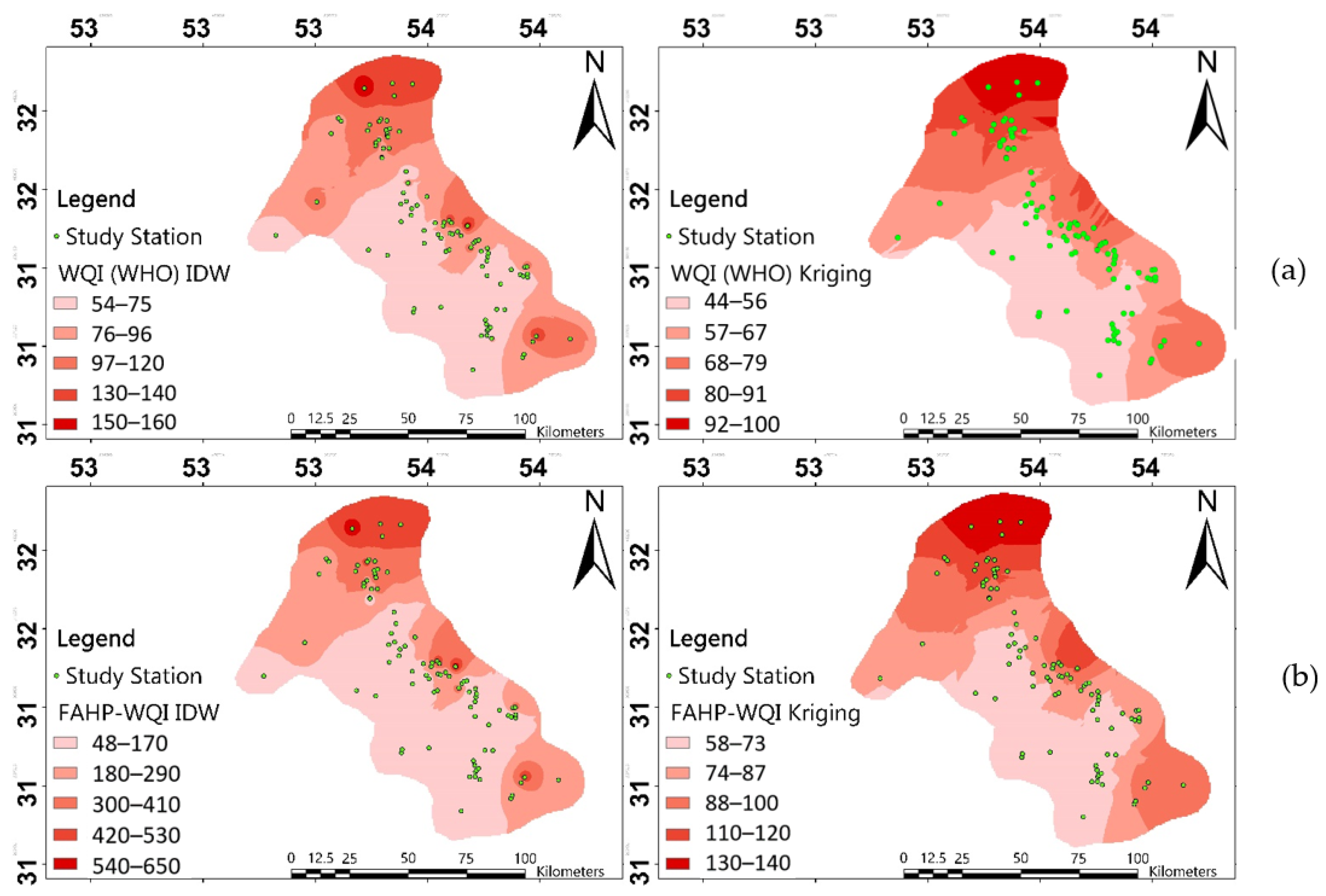
The drinking water quality in the study area was evaluated using the WQI index. Moreover, the FAHP-WQI method was used to resolve the inconsistencies in the WQI method. Figure 2 shows the water quality index within the study area, calculated by means of the Kriging and IDW interpolation methods. As seen in Figure 2, based on the WQI(WHO) analysis more than 78% of the surface of the Ardakan-Yazd case study area was classified in the excellent or good classes.

As can be observed in Figure 2, according to the WQI(WHO) analysis 72 wells out of 96 were in a good class regarding water quality, while 23 wells were in a poor class. Furthermore, the southwestern and central regions of the study area had higher-quality drinking water resources compared to the northern and southeastern regions. According to the FAHP-WQI results, 31 water wells out of 96 water wells were in a good class regarding water quality, 23 wells were in the poor class, 22 wells were in the unusable class, and four wells were in the excellent class.

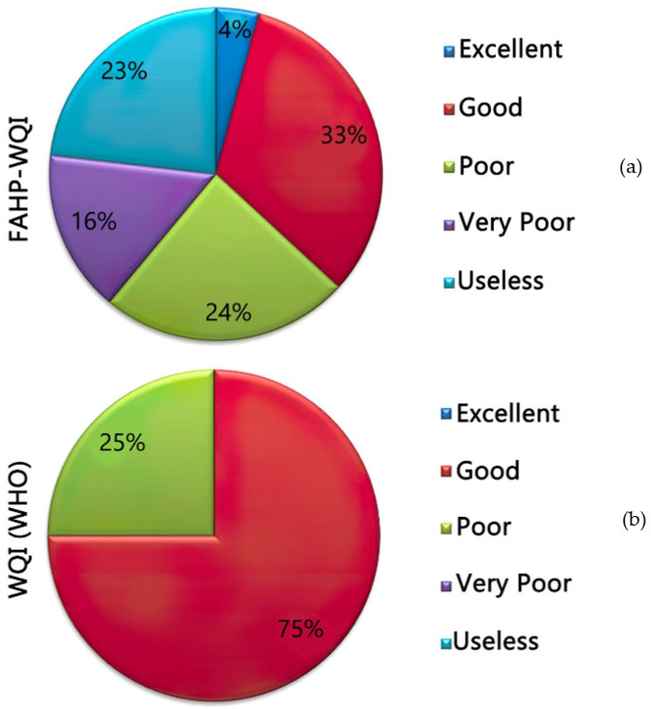
This could be due to the existence of urban areas and the existence of absorptive wells in these parts of the study area. The location of the main wells used for quality assessment in the study area are highlighted in green color. As discussed earlier, the use of the WQI(WHO) method has inconsistencies, but, compared to the FAHP-, more than 60% of the case study areas of Ardakan-Yazd were classified within excellent or good classes. Different interpolation methods used in this study included IDW and ordinary Kriging. The results of classification of the wells under study into five categories of excellent, good, poor, very poor, and unusable, using the WQI(WHO), and FAHP-WQI methods, are presented in Figure 3. According to the WQI-based rankings, after using the FAHP-WQI model, the results were subject to a lot of changes. Such changes could typically be seen in the vicinity of wells with approximately equal WQI values. When a sample with a lower WQI value had a chemical parameter with a much higher value than other samples with lower WQI degrees, effects, such as those mentioned, became more apparent. Using the Fuzzy Analytic Hierarchy Process method (FAHP), along with WQI, increased the accuracy in weighting parameters and reduced the amount of uncertainty in the water quality calculations.

3.2. Chemical Indicators

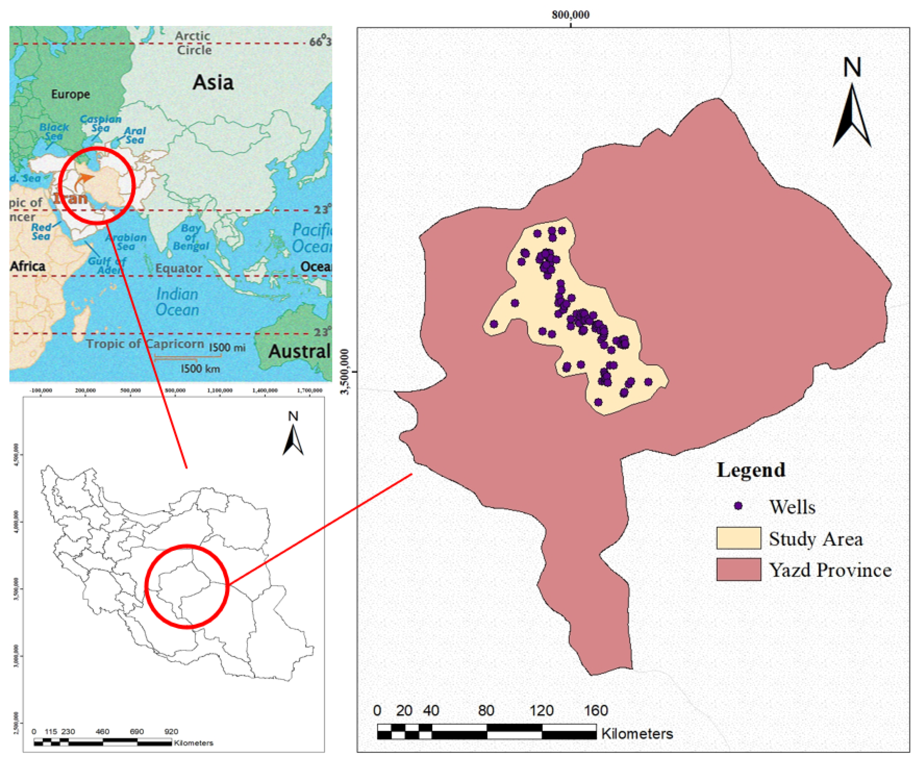
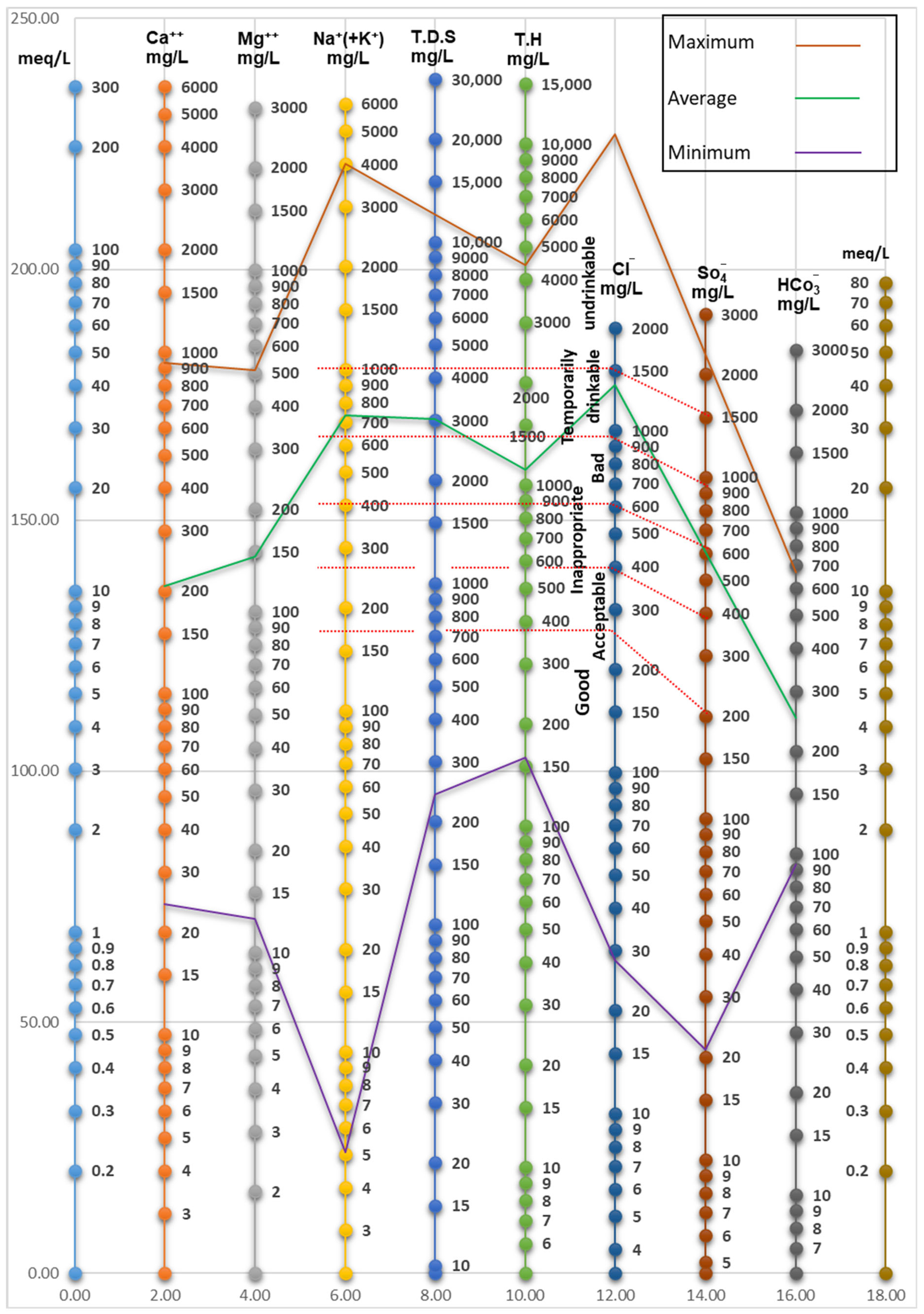
To investigate the hydro-geochemistry of groundwaters in the Yazd-Ardakan plain, water samples were collected from 96 agricultural and drinking wells. The samples were collected with the aid of Yazd Agricultural Jihad Management Organization and transferred to the Soil and Water Laboratory of Yazd province for further chemical analysis. the parameters measured in this study included the amounts of calcium (${\mathrm{ca}}^{2+}$), magnesium (${\mathrm{mg}}^{2+}$), sodium (${\mathrm{Na}}^{+}$), bicarbonate (${\mathrm{Hco}}_3^{-}$), sulfate (${\mathrm{SO}}_4$), chloride (${\mathrm{Cl}}^{-}$), ec, potassium (${\mathrm{K}}^{+}$), total dissolved solids (tds), total hardness (th), and acidity. Data Quality Assurance and Quality Control (QA/QC) processes were considered throughout the study. Approximately half of the prepared sample volume was specifically and individually checked in the laboratory to ensure QA/QC mechanisms. The accuracy of chemical analysis was confirmed by charge balance errors, and samples were <5% error.

The statistical characteristics of the water of the wells used, along with their standard ranges for the water, are presented in Table 6. This Table shows that the average of the parameters, pH, HCO₃, Ca, Na, and SO₄, were all located within the normal and standard ranges, but the parameters, EC, TDS, mg, and Ca, were above the allowable standard upper bounds. Despite the average of some samples being in the standard range, the maximum values of all parameters showed that there were areas in the study area that are not suitable for irrigation purposes. The high values of EC and TDS in this plain are due to the existence of salt formations, the amount of water input to the aquifer and the amount of water harvested from it. The electrical conductivity of irrigation water or soil saturation extractives are indicators of the amount of minerals dissolved in the soil environment, and, as such, determine the quality and classification of water and soil in terms of salinity. Therefore, EC must be measured in all studies and research regarding the salinity of water and soil [50]. The electrical conductivity of groundwater in the region under study was in the range of 375–19,960 μmho/cm, and the average EC value was equal to 4878.21. The total dissolved solid in the study area was also in the range of 240–12,000 mg/L, and the average TDS was equal to 3017.78. As shown in Figure 4a, the results of constructing a zoning map of the parameters under investigation indicated that, for parameters EC and TDS, the quality of water was not suitable for agriculture in most areas of Yazd-Ardakan plain. In fact, 47.36% of the wells in this plain were in poor condition, according to the EC indicator. Moreover, regarding the parameter TDS, 45.26% of the wells were in poor conditions The salinity in Yazd-Ardakan plain followed a decreasing trend from east to west. There was also a decreasing trend from north to south. The satisfactory water quality in the central and western regions is mainly due to the existence of rocks formed in these regions, because these parts have Eocene-aged rocks of andesite, latite, ignimbrite, and basalt, for which the existing waters are mainly fresh water.

Classification of irrigation water in terms of chloride concentration is necessary due to the special sensitivity of some plants to chloride. Some results showed that a large part (about 38%) of the plain had a concentration higher than the allowable limits. Chloride concentration varies in the range of 0.79 to 208.68 mEq/L and its average for the Yazd-Ardakan plain was equal to 38.39. Chloride had a decreasing trend from east to west and from north to south, Figure 4b. The probable reasons for rising groundwater Cl concentrations include mixing new waters with higher Cl concentrations, which are mainly of four types: deep liquids, hydrothermal waters, porous water in sea clays, and contaminated surface waters [51,52].

The PS indicator reflects the impact of high salt concentrations with respect to chloride and sulfate and increases with the reduction of soil moisture. The water is classified into three classes: good PS (less than 3 mmol/L), average PS (3 to 15 mmol/L) and unusable PS (higher than 15 mmol/L). Using this index, the majority of wells were in the poor range and 41% had no problems in irrigation systems. The decrease in water quality of northern and southern areas with respect to salinity was obvious. Examining the qualitative data from the wells showed that the minimum, maximum and average values were 0.22, 173.99, and 31.81, for sodium, 1.03, 41.82, and 11.88, for magnesium, and 1.2, 46.31, and 10.27 mEq/L for calcium, respectively. This means that 23.15%, 61.05%, and 14.73% of the wells were in poor condition according to these parameters, respectively. The reason for high amounts of magnesium ions and a high percentage of magnesium ions in the water of the wells under investigation is due to reactions to the rocks and geological formations.

Table 6. Statistical characteristics of well water used, along with their standards [53].

SO4	Cl−	Na+	Mg2+	Ca2+	HCO3	TDS	pH	Ec	Parameter
meq∙L−1						mg∙L−1	-	mmoh cm−1
45.8	208.68	173.99	41.82	46.31	10.96	12,000	8.75	19,960	Maximum
0.42	0.79	0.22	1.03	1.2	1.52	240	7	375	Minimum
12.08	38.39	31.81	11.88	10.27	4.09	3017.78	7.82	4878.21	Average
10.91	45.37	37.52	10.74	9.33	1.77	2918.01	0.31	4740.49	Standard deviation
0–20	0–30	0–40	0–5	0–20	0–10	0–2000	6.5–8	0–3000	Standard domain

Table 6. Statistical characteristics of well water used, along with their standards [53].

SO4	Cl−	Na+	Mg2+	Ca2+	HCO3	TDS	pH	Ec	Parameter
meq∙L−1						mg∙L−1	-	mmoh cm−1
45.8	208.68	173.99	41.82	46.31	10.96	12,000	8.75	19,960	Maximum
0.42	0.79	0.22	1.03	1.2	1.52	240	7	375	Minimum
12.08	38.39	31.81	11.88	10.27	4.09	3017.78	7.82	4878.21	Average
10.91	45.37	37.52	10.74	9.33	1.77	2918.01	0.31	4740.49	Standard deviation
0–20	0–30	0–40	0–5	0–20	0–10	0–2000	6.5–8	0–3000	Standard domain

Bicarbonate is an important parameter due to the deposition of calcium and magnesium in soil and water, as their deposition increases SAR and intensifies the sodium problem. The amounts of carbonate (CO₃) and bicarbonate (HCO₃) are in equilibrium within ground waters. However, carbonate is released from under the ground immediately after water outflow. Examinations of the data obtained from the wells under study showed that the minimum, maximum and average values were equal to 1.52, 10.96, and 4.09 for bicarbonate, 0.42, 45.8, and 12.08 mEq/L for sulfate, respectively. Equivalence maps of bicarbonate and sulfate values for the Yazd-Ardakan plain were plotted using the ordinary Kriging method and are presented in Figure 4c.

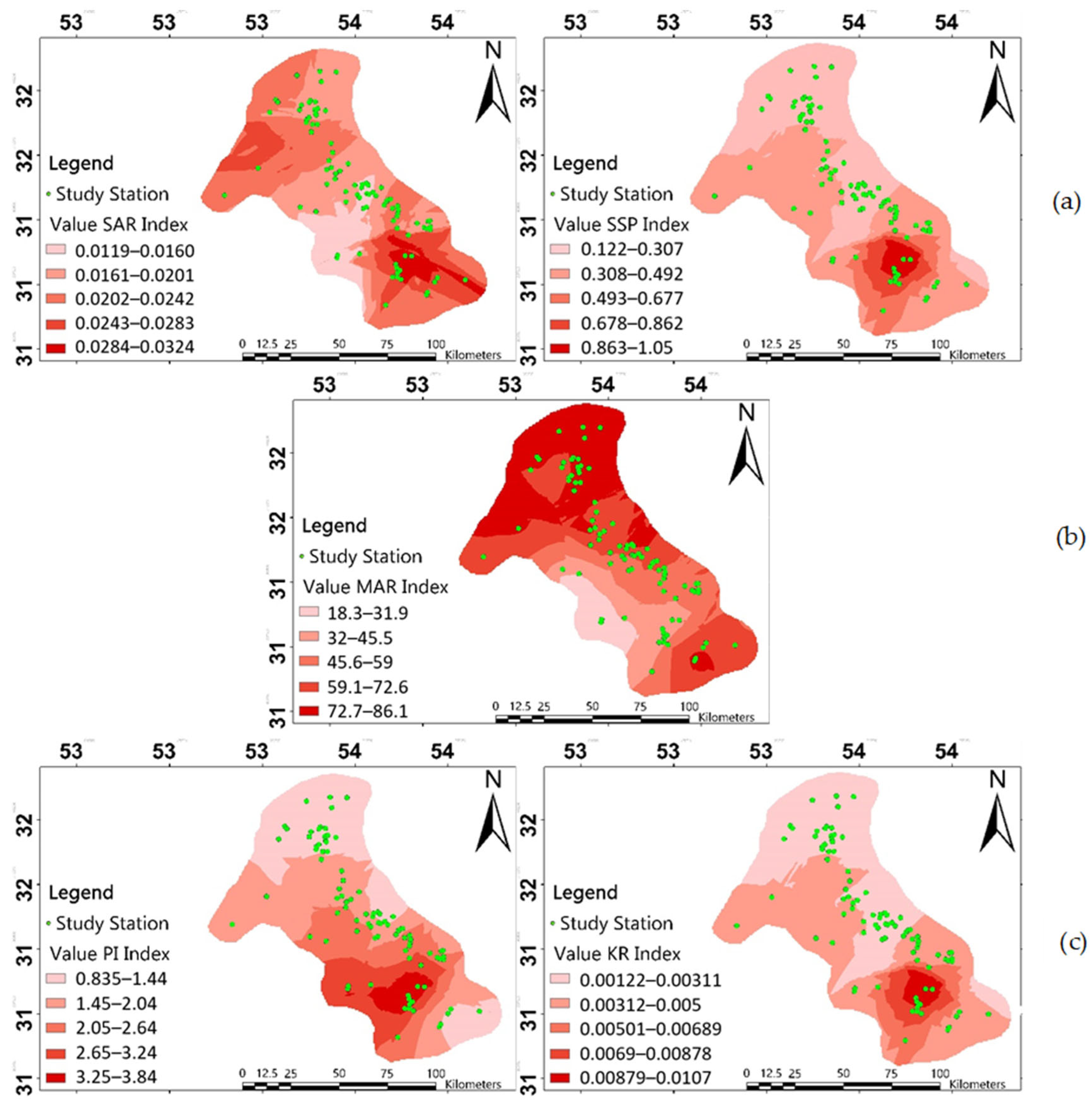
In the past, water quality was only assessed based on sodium. The truth is that sodium has highly negative effects on soil and plant growth. One way to determine the risk of sodium is to use the sodium absorption ratio. This method was proposed by the American Salinity Laboratory. The minimum, maximum, and average sodium absorption ratios in the Yazd-Ardakan plain were equal to 0.15, 30.9, and 8.37, respectively. Studies suggest that, except for a few cases, waters from other wells had SAR values less than 15, which are within the appropriate range in this regard. This means that 16.9% of the wells were in dire condition in this regard. The values of this index are presented in Figure 4b, along with the PS index. The calculated total quality index showed that 18.53% of the regions in the Yazd-Ardakan plain had appropriate water quality for irrigation, 65.28% had average water quality, while 18.17% had poor water quality. The SSP ratio, or the percentage of sodium dissolved in water, was calculated using the concentrations of calcium, sodium, and magnesium elements. SSP is an important parameter for investigating salinity risk. High percentages of soluble sodium may prevent plant growth and reduce soil permeability. The maximum, minimum, and average values of the soluble sodium percentage in the Yazd-Ardakan plain were equal to 86.05, 5.05, and 49.08, respectively. The SAR and SSP index zoning map using Kriging interpolation is presented in Figure 5a. The results showed that 66.31% of the well water had SSP values higher than 40%. The study of spatial changes of this index also showed that its value increased from east to west and from north to south of the plain. The bar diagram of the SSP index and the MAR index of water from wells in the region are presented in Figure 5. The permissible limit of the MAR parameter for irrigation water is 50% [54]. Most of the samples under study were above the standard allowable limit of 50% with respect to magnesium absorption ratio. This value reached 60% in some wells, and instances of 80% were also observed in a few wells. The study of zoning of this index, depicted in Figure 5, showed that the groundwater from the northern areas of the zone had the worst conditions in this regard. Higher magnesium amounts in water not only result in water salinity, but also reduce product yields [32].

The average Kelley’s ratio for the water of the wells under study was determined to be equal to 1.03. In general, the situation was relatively favorable with respect to this indicator, since Chidambaram et al. [55] reported that the maximum allowable limit for this component in water is equal to 1. If this ratio became greater than one, it would indicate that the amount of sodium was higher than the two divalent elements of calcium and magnesium, and it would damage soil permeability in the long term. Examining the spatial changes of Kelley’s index in Figure 5c, the southern areas of the plain were not satisfactory, and the soil permeability had been damaged. The bar diagram of the Kr index, as well as the EC index, along with their allowable limits, are illustrated in Figure 5.

To investigate the permeability of another index that covers more factors compared to Kelley’s ratio, the permeability index was used. Of course, this index is affected by the long-term use of irrigation water. According to a report by Chidambaram et al. [55], the appropriate range for the permeability index is from 0.19 to 7.15. Figure 5c presents the equivalence map of the PI and KR indices throughout the Yazd-Ardakan plain. Examining the spatial variations of PI, the ground waters of this plain had no issues in this regard, but, unlike previous indices, the values for this index were at their highest in the southern and southwestern regions.

Improving groundwater quality, or mitigating the effects of poor water quality, can be complex. In the following, a few suggestions are presented for improving groundwater quality in the study area: (i) implementing Best Management Practices (BMPs). These practices can include reducing the use of fertilizers and pesticides in the agricultural sector and proper waste management; (ii) management of human activities, such as mining, overexploitation of groundwater, and landfilling, which can significantly influence groundwater quality. Proper management and regulation of these activities can help prevent groundwater pollution.

3.3. Wilcox and Schoeller Diagrams

As stated earlier, the Wilcox diagram presents the classification of water quality in terms of agriculture. According to Figure 6, about 37.25% of the wells were in classes C3S2, and C3S1, which was, in fact, the highest accumulation in this area and indicated waters with poor quality that were only effective for irrigating certain crops in large textured lands with proper drainage. Moreover, about 16.25% of the wells were classified in the C4S4 class, which indicated very poor water quality for irrigation purposes. Only about 13.75% of the wells were determined to have average water quality. The Schoeller diagram is presented in Figure 7. The minimum, maximum and average amounts of ions deliver a classification of drinking water quality. According to the diagram, the drinking water quality in the Yazd- Ardakan plain was classified as acceptable, bad, and unsuitable.

3.4. Assessment of AL Models in WQI Prediction

From 96 data sets, 70% (66 data sets) were randomly selected for training and 30% (30 data sets) for testing. Eleven main variables, SO₄, Cl, HCO₃, pH, TDS, TH, EC, K, Na, Mg and Ca, were used to develop GEP, M5P and MARS.

3.4.1. GEP Model

In the GEP algorithm, empirical relationships are generated to predict continuous values using a combination of mathematical functions and mathematical operators [56].

Since GEP uses mathematical functions and operators, the empirical relations of this algorithm also include linear and non-linear combinations of mathematical functions and operators. For example, empirical GEP relationships may involve linear combinations of mathematical functions such as addition, multiplication, and subtraction. These relations may also include non-linear combinations of mathematical functions, such as logarithmic and power functions [57]. To evaluate WQI using the GEP model, the first step in implementing the model is to find the best input model to the model, based on which the best output is obtained. The pattern that causes the least error is considered the most appropriate input pattern among the different input patterns. Of the data, 70% was used to train the model using the random selection method, and the remaining 30% was used to validate the model. All the data were introduced as input to the software to find the best structure as input for WQI estimation. The software introduced the best input combination by running the model with different input combinations. The GEP model expression trees are shown in Figure 8. One of the important capabilities of GEP is to present mathematical relationships explicitly and simply. The simplified analytical form of the GEP model can be expressed as in Equation (18).

$$\begin{array}{cc}\hfill \mathrm{WQI}=\left(\right((-7.41& +\hspace{0.17em}pH)\times (HCO3+HCO3\left)\right)-(\left(-0.832-pH\right)-(-9.796\hfill \\ & +\left(-9.796\right)\left)\right))+(\left(\right(\left(9.18\times pH\right)+(Na\hfill \\ & -\left(-5.537\right)\left)\right)\times \left(pH\times K\right))\times 0.185)+\left(\right(HCO3\hfill \\ & -\left(8.303\times 2.324\right))+\left(\left(K+Mg\right)+\left(pH\times pH\right)\right))\hfill \end{array}$$

(18)

3.4.2. M5P Tree Model

The M5P algorithm, like MARS, is a non-parametric regression algorithm used to predict continuous values. This algorithm also estimates the relationship between dependent and independent variables using linear and non-linear basis functions. Unlike MARS, which uses a polynomial and interactive basis function in its primary function, the M5P algorithm uses a decision tree in its primary function [43,58,59].

The evaluation results of the M5P tree model show the high accuracy of this model. One of the advantages of the M5P tree model is to provide a simple linear relationship combination in the form of a tree model that can be used to estimate the water quality index. Generating a tree model in the first step includes determining the most appropriate input parameter for branching and the division rule to produce a decision tree. Therefore, after entering all the inputs in the Weka software (version 3.9.3), SO₄, Cl, HCO₃, pH, K, and Na parameters were selected as the best input combination. Since the results of this model are in the form of regression relationships, the regression model is presented according to Equation (19).

$$\begin{array}{cc}\hfill \mathrm{WQI}=0.6654& \times SO4+0.3761\times Cl+2.1054\times HCO3\hfill \\ & +33.2017\times PH+117.0444\times K-0.0736\times Na\hfill \\ & -232.1628\hfill \end{array}$$

(19)

3.4.3. MARS Model

The MARS model is implemented in Matlab R2013a software. This model can provide the best combination of model inputs for WQI estimation. Hence, the best proposed input combination included Ec, pH, K, HCO₃, SO₄, Cl, and TH parameters. Leading and trailing phases were used for prediction. In this research, the number of basic functions (NBF) equaled 14 functions, introduced with the symbol λ. In the implementation of this model, GCV equal to 0.1375 was obtained. The basic functions of this model are calculated in

Table 7. Fixed coefficients and basic functions obtained from the MARS model.

Fixed Coefficients		Basis Functions
C1	0.00065043	${\lambda }_1$	max (0, Ec—2950)
C2	−0.00068293	${\lambda }_2$	max (0, 2950—Ec)
C3	33.358	${\lambda }_3$	max (0, pH—7.8)
C4	−33.391	${\lambda }_4$	max (0, 7.8—pH)
C5	116.88	${\lambda }_5$	max (0, K—0.05)
C6	−113.52	${\lambda }_6$	max (0, 0.05—K)
C7	1.9707	${\lambda }_7$	max (0, HCO3—2.96)
C8	−1.8072	${\lambda }_8$	max (0, 2.96—HCO3)
C9	0.54801	${\lambda }_9$	max (0, SO4—20.82)
C10	−0.52785	${\lambda }_{10}$	max (0, 20.82—SO4)
C11	0.24887	${\lambda }_{11}$	max (0, Cl—65.99)
C12	−0.24965	${\lambda }_{12}$	max (0, 65.99—Cl)
C13	0.0011579	${\lambda }_{13}$	max (0, TH—2659)
C14	−0.0014433	${\lambda }_{14}$	max (0, 2659—TH)

, and the general relation extracted from the mentioned model for estimation is also obtained according to Equation (20):

$$\Gamma \left(t\right)=71.663+{\displaystyle \sum }_{i=1}^{14}{C}_i\cdot {\lambda }_i\left(t\right)$$

(20)

Table 8. Performance of ML models.

		R	RMSE	MAE	NSE	Ia
GEP	Training	0.986	4.366	2.884	0.971	0.993
	Testing	0.980	5.557	3.973	0.920	0.975
M5p	Training	0.999	0.286	0.196	0.999	1.000
	Testing	1.000	0.225	0.175	0.999	1.000
MARS	Training	1.000	0.172	0.127	1.000	1.000
	Testing	0.999	0.212	0.167	0.999	1.000

shows the values of error evaluation criteria for machine learning models in two parts, training and testing. According to the error evaluation criteria in the mentioned table among machine learning models, the performance of the MARS model was better than that of the other models. In the M5P model, the values of RMSE, MAE, and Ia for the test data were obtained as 0.225, 0.175, and 1, respectively. The training data of this model had acceptable accuracy and was close to the test results. These results showed that the mentioned model could estimate the training and testing data well. Among the models, the performance of GEP had the lowest prediction accuracy compared to other models. Of course, according to the evaluation criteria, it could be said that the results of GEP were weaker than other models, but it had high accuracy in predicting the water quality index. The MARS model also had good estimation accuracy, and the error evaluation indices showed better values, with a slight difference compared to the M5P model (Table 8). In the examination of statistical error values in the two categories of training and testing data in the models, it was observed that there was a slight difference between the error of training and testing data in MARS and M5P models compared to GEP. Figure 9 shows the observed values against the predicted values of the models in the training and test section. The observed and predicted values by MARS and M5p models were closest to the bisector line, showing good convergence. Among the models, GEP had relatively scattered data, which caused a lower correlation coefficient. The MARS model had decreased accuracy in the testing phase compared to the training phase, but it still had the best values among the statistical indicators, compared to the other two models.

The results of this research were compared with the studies of other researchers. In a study conducted by Amiri-Ardakani and Najafzadeh [60], the records of broken pipes and related causes in the water distribution networks of Yazd City were investigated. In this study, three models, GEP, MARS, and M5, were used to derive the exact formula for estimating the failure rate of pipes. The results also showed that the MARS model performed more satisfactorily than other models. In another study, Mehdizadeh, et al. [61] estimated Iran’s monthly mean evaporation and transpiration. They used GEP, MARS, and two Support Vector Machine (SVM) models. The results showed that MARS and SVM-RBF methods performed better than GEP and SVM-Poly. In other research, Qasem, et al. [62] investigated the ability of three data-driven methods, (GEP), M5 model tree, and support vector regression (SVR), to model and estimate dew point temperature (DPT) in Tabriz station, Iran. In the end, the M5 model was recommended as the most accurate model in DPT estimation compared to other models considered.

For future studies, it is suggested to investigate the sources of uncertainty, both metric critical value uncertainties and weight uncertainties in WQI and control them as much as possible. Both producers and consumers of water bear the costs of a lack of water supply, or the supply of low-quality water, so, investigating the sources of future uncertainties, along with water quality checks to investigate different water supply systems, should be a basis for analyzing the costs and effects of risk control [63].

4. Conclusions

In this study, WQI(WHO) and Fuzzy AHP-WQI were used to check the quality of 96 wells in the Yazd-Ardakan Plain and then the results of these two methods were compared. According to the results of the WQI(WHO) method, it was found that 72 wells out of 96 wells were in the good class, in terms of water quality, and 23 wells were classified as poor in the WQI analysis. Meanwhile, according to the FAHP-WQI method, 31 wells were in the good class, 23 wells were in the poor classification, 22 wells were in the unusable category, and 4 wells were in the excellent category of the WQI analysis. Wilcox and Schoeller’s diagrams were also used to classify water quality from the point of view of agriculture and to evaluate the water from the point of view of drinkability, respectively. According to the results of the Wilcox diagram, it was found that about 37.25% of the wells were in the C3S2 and C3S1 classes, indicating low-quality water that is only effective for irrigating some crops in large-textured fields with proper drainage. According to Schoeller’s diagram, the drinking water quality of the Yazd-Ardakan Plain was classified into three categories: acceptable, bad, and inappropriate. Since calculating the water quality index takes time, artificial intelligence algorithms were used in this research to estimate WQI. Three models, GEP, M5P, and MARS, were selected, and a WQI calculation was performed according to the processes of each algorithm. The results from the three models were evaluated using Nash–Sutcliffe (NSE), root mean square error (RMSE), agreement index (Ia), correlation coefficient (R), and mean absolute error (MAE) statistical indices. Finally, the models were compared to determine the best model for estimating the water quality index. GEP had relatively scattered data, which caused a lower correlation coefficient than the other two models. The results of the statistical indicators for the M5P and MARS models were close. The results of the MARS model for the RMSE, MAE, Ia, NSE, and R indicators in the training phase were equal to 0.172, 0.127, 1, 1 and 1, respectively, and for the test phase, they were equal to 0.212, 0.167, 1, 0.999 and 0.999. The accuracy of the MARS model decreased in the testing phase compared to the training phase, but it still had the best values among the statistical indicators, compared to the other two models.

References

1. Aghazadeh, N.; Asghari Moghaddam, A. Assessment of Groundwater Quality and its Suitability for Drinking and Agricultural Uses in the Oshnavieh Area, Northwest of Iran. J. Environ. Prot. 2010, 1, 30–40. [Google Scholar] [CrossRef]
2. Moridi, A. State of Water Resources in Iran. Int. J. Hydrol. 2017, 1, 111–114. [Google Scholar] [CrossRef]
3. Moshir Panahi, D.; Kalantari, Z.; Ghajarnia, N.; Seifollahi-Aghmiuni, S.; Destouni, G. Variability and change in the hydro-climate and water resources of Iran over a recent 30-year period. Sci. Rep. 2020, 10, 7450. [Google Scholar] [CrossRef]
4. Horton, R.K. An index number system for rating water quality. J. Water Pollut. Control Fed. 1965, 37, 300–306. [Google Scholar]
5. Rickwood, C.J.; Carr, G.M. Development and sensitivity analysis of a global drinking water quality index. Environ. Monit. Assess. 2009, 156, 73–90. [Google Scholar] [CrossRef]
6. Wilcox, L.V. The Quality of Water for Irrigation Use; Technical Bulletin; US Department of Agriculture: Washington, DC, USA, 1948; 19p.
7. ISIRI. Drinking Water: Physical and Chemical Specifications; ISIRI No. 1053; ISIRI: Tehran, Iran, 2010; p. 26. Available online: https://scholar.google.com/scholar_lookup?title=Drinking+Water:+Physical+and+Chemical+Specifications+(ISIRI+No.+1053)&publication_year=2010& (accessed on 1 January 2023).
8. WHO. Guidelines for Drinking-Water Quality; World Health Organization: Geneva, Switzerland, 2011; Volume 216, pp. 303–304. [Google Scholar]
9. Baghvand, A.; Nasrabadi, T.; Bidhendi, G.N.; Vosoogh, A.; Karbassi, A.; Mehrdadi, N. Groundwater quality degradation of an aquifer in Iran central desert. Desalination 2010, 260, 264–275. [Google Scholar] [CrossRef]
10. Kura, N.U.; Ramli, M.F.; Sulaiman, W.N.A.; Ibrahim, S.; Aris, A.Z.; Narany, T.S. Spatiotemporal Variations in Groundwater Chemistry of a Small Tropical Island Using Graphical and Geochemical Models. Procedia Environ. Sci. 2015, 30, 358–363. [Google Scholar] [CrossRef]
11. Saka, D.; Akiti, T.T.; Osae, S.; Appenteng, M.K.; Gibrilla, A. Hydrogeochemistry and isotope studies of groundwater in the Ga West Municipal Area, Ghana. Appl. Water Sci. 2013, 3, 577–588. [Google Scholar] [CrossRef]
12. Zadeh, L.A.; Klir, G.J.; Yuan, B. Fuzzy Sets, Fuzzy Logic, and Fuzzy Systems; World Scientific: Singapore, 1996; Volume 6, p. 840. [Google Scholar]
13. Gharibi, H.; Mahvi, A.H.; Nabizadeh, R.; Arabalibeik, H.; Yunesian, M.; Sowlat, M.H. A novel approach in water quality assessment based on fuzzy logic. J. Environ. Manag. 2012, 112, 87–95. [Google Scholar] [CrossRef] [PubMed]
14. Kouadri, S.; Elbeltagi, A.; Islam, A.R.M.T.; Kateb, S. Performance of machine learning methods in predicting water quality index based on irregular data set: Application on Illizi region (Algerian southeast). Appl. Water Sci. 2021, 11, 190. [Google Scholar] [CrossRef]
15. Palani, S.; Liong, S.-Y.; Tkalich, P. An ANN application for water quality forecasting. Mar. Pollut. Bull. 2008, 56, 1586–1597. [Google Scholar] [CrossRef]
16. Bashi-Azghadi, S.; Kerachian, R.; Bazargan-Lari, M.R.; Solouki, K. Characterizing an unknown pollution source in groundwater resources systems using PSVM and PNN. Expert Syst. Appl. 2010, 37, 7154–7161. [Google Scholar] [CrossRef]
17. Lumb, A.; Sharma, T.C.; Bibeault, J.-F. A Review of Genesis and Evolution of Water Quality Index (WQI) and Some Future Directions. Water Qual. Expo. Health 2011, 3, 11–24. [Google Scholar] [CrossRef]
18. Gazzaz, N.M.; Yusoff, M.K.; Aris, A.Z.; Juahir, H.; Ramli, M.F. Artificial neural network modeling of the water quality index for Kinta River (Malaysia) using water quality variables as predictors. Mar. Pollut. Bull. 2012, 64, 2409–2420. [Google Scholar] [CrossRef]
19. Boateng, T.K.; Opoku, F.; Acquaah, S.O.; Akoto, O. Groundwater quality assessment using statistical approach and water quality index in Ejisu-Juaben Municipality, Ghana. Environ. Earth Sci. 2016, 75, 489. [Google Scholar] [CrossRef]
20. Adimalla, N.; Qian, H. Spatial distribution and health risk assessment of fluoride contamination in groundwater of Telangana: A state-of-the-art. Geochemistry 2020, 80, 125548. [Google Scholar] [CrossRef]
21. Ben Brahim, F.; Boughariou, E.; Bouri, S. Multicriteria-analysis of deep groundwater quality using WQI and fuzzy logic tool in GIS: A case study of Kebilli region, SW Tunisia. J. Afr. Earth Sci. 2021, 180, 104224. [Google Scholar] [CrossRef]
22. Khoi, D.N.; Quan, N.T.; Linh, D.Q.; Nhi, P.T.T.; Thuy, N.T.D. Using Machine Learning Models for Predicting the Water Quality Index in the La Buong River, Vietnam. Water 2022, 14, 1552. [Google Scholar] [CrossRef]
23. YRW Organization. Report on the Continuation of Groundwater Studies; Ardakan: Yazd, Iran, 1992. [Google Scholar]
24. Goodarzi, M.R.; Abedi, M.J.; Niknam, A.R.R.; Heydaripour, M. Groundwater quality status based on a modification of water quality index in an arid area, Iran. Water Supply 2022, 22, 6245–6261. [Google Scholar] [CrossRef]
25. Prasad, M.; Sunitha, V.; Reddy, Y.S.; Suvarna, B.; Reddy, B.M.; Reddy, M.R. Data on water quality index development for groundwater quality assessment from Obulavaripalli Mandal, YSR district, A.P India. Data Brief 2019, 24, 103846. [Google Scholar] [CrossRef] [PubMed]
26. Wu, J.; Xue, C.; Tian, R.; Wang, S. Lake water quality assessment: A case study of Shahu Lake in the semiarid loess area of northwest China. Environ. Earth Sci. 2017, 76, 232. [Google Scholar] [CrossRef]
27. Babanezhad, E.; Qaderi, F.; Salehi Ziri, M. Spatial modeling of groundwater quality based on using Schoeller diagram in GIS base: A case study of Khorramabad, Iran. Environ. Earth Sci. 2018, 77, 339. [Google Scholar] [CrossRef]
28. Vadiati, M.; Asghari-Moghaddam, A.; Nakhaei, M.; Adamowski, J.; Akbarzadeh, A.H. A fuzzy-logic based decision-making approach for identification of groundwater quality based on groundwater quality indices. J. Environ. Manag. 2016, 184, 255–270. [Google Scholar] [CrossRef] [PubMed]
29. Soleimani, H.; Abbasnia, A.; Yousefi, M.; Mohammadi, A.A.; Khorasgani, F.C. Data on assessment of groundwater quality for drinking and irrigation in rural area Sarpol-e Zahab city, Kermanshah province, Iran. Data Brief 2018, 17, 148–156. [Google Scholar] [CrossRef]
30. Delgado, C.; Pacheco, J.; Cabrera, A.; Batllori, E.; Orellana, R.; Bautista, F. Quality of groundwater for irrigation in tropical karst environment: The case of Yucatán, Mexico. Agric. Water Manag. 2010, 97, 1423–1433. [Google Scholar] [CrossRef]
31. Richards, L.A. Diagnosis and Improvement of Saline and Alkali Soils; LWW: Philadelphia, PA, USA, 1954. [Google Scholar]
32. Joshi, D.M.; Kumar, A.; Agrawal, N. Assessment of the irrigation water quality of river Ganga in Haridwar district. Rasayan J. Chem. 2009, 2, 285–292. [Google Scholar]
33. Doneen, L. Water Quality for Agriculture, Department of Irrigation; University of California: Davis, CA, USA, 1964; Volume 48. [Google Scholar]
34. Kelley, W. Use of saline irrigation water. Soil Sci. 1963, 95, 385–391. [Google Scholar] [CrossRef]
35. van Laarhoven, P.J.M.; Pedrycz, W. A fuzzy extension of Saaty’s priority theory. Fuzzy Sets Syst. 1983, 11, 229–241. [Google Scholar] [CrossRef]
36. Chang, D.-Y. Applications of the extent analysis method on fuzzy AHP. Eur. J. Oper. Res. 1996, 95, 649–655. [Google Scholar] [CrossRef]
37. Şener, E.; Şener, Ş. Evaluation of groundwater vulnerability to pollution using fuzzy analytic hierarchy process method. Environ. Earth Sci. 2015, 73, 8405–8424. [Google Scholar] [CrossRef]
38. Tseng, M.-L.; Lin, Y.-H.; Chiu, A.; Chen, C.Y. Fuzzy AHP-approach to TQM strategy evaluation. IEMS 2008, 7, 34–43. [Google Scholar]
39. Goodarzi, M.R.; Niknam, A.R.R.; Jamali, V.; Pourghasemi, H.R. Aquifer vulnerability identification using DRASTIC-LU model modification by fuzzy analytic hierarchy process. Model. Earth Syst. Environ. 2022, 8, 5365–5380. [Google Scholar] [CrossRef]
40. Niazkar, M. Chapter 19—Multigene genetic programming and its various applications. In Handbook of Hydroinformatics; Eslamian, S., Eslamian, F., Eds.; Elsevier: Amsterdam, The Netherlands, 2023; pp. 321–332. [Google Scholar]
41. Bateni, S.; Jeng, D.-S. Estimation of pile group scour using adaptive neuro-fuzzy approach. Ocean Eng. 2007, 34, 1344–1354. [Google Scholar] [CrossRef]
42. Ali Khan, M.; Zafar, A.; Akbar, A.; Javed, M.F.; Mosavi, A. Application of Gene Expression Programming (GEP) for the Prediction of Compressive Strength of Geopolymer Concrete. Materials 2021, 14, 1106. [Google Scholar] [CrossRef]
43. Quinlan, J.R. Learning with Continuous Classes. In Proceedings of the Australian Joint Conference on Artificial Intelligence, Hobart, Australia, 16–18 November 1992; pp. 343–348. [Google Scholar]
44. Wang, Y.; Witten, I.H. Inducing model trees for continuous classes. In Proceedings of the Ninth European Conference on Machine Learning, Prague, Czech Republic, 23–25 April 1997; pp. 128–137. [Google Scholar]
45. Khosravi, K.; Golkarian, A.; Booij, M.J.; Barzegar, R.; Sun, W.; Yaseen, Z.M.; Mosavi, A. Improving daily stochastic streamflow prediction: Comparison of novel hybrid data-mining algorithms. Hydrol. Sci. J. 2021, 66, 1457–1474. [Google Scholar] [CrossRef]
46. Friedman, J.H. Multivariate adaptive regression splines. Ann. Stat. 1991, 19, 1–67. [Google Scholar] [CrossRef]
47. Lasheras, F.S.; Nieto, P.J.G.; De Cos Juez, F.J.; Bayón, R.M.; Suárez, V.M.G. A Hybrid PCA-CART-MARS-Based Prognostic Approach of the Remaining Useful Life for Aircraft Engines. Sensors 2015, 15, 7062–7083. [Google Scholar] [CrossRef]
48. Niazkar, M. Assessment of artificial intelligence models for calculating optimum properties of lined channels. J. Hydroinformatics 2020, 22, 1410–1423. [Google Scholar] [CrossRef]
49. Niazkar, M.; Goodarzi, M.R.; Fatehifar, A.; Abedi, M.J. Machine learning-based downscaling: Application of multi-gene genetic programming for downscaling daily temperature at Dogonbadan, Iran, under CMIP6 scenarios. Theor. Appl. Climatol. 2023, 151, 153–168. [Google Scholar] [CrossRef]
50. Hardie, M.; Doyle, R. Measuring Soil Salinity. In Plant Salt Tolerance: Methods and Protocols; Shabala, S., Cuin, T.A., Eds.; Humana Press: Totowa, NJ, USA, 2012; pp. 415–425. [Google Scholar]
51. Skelton, A.; Andrén, M.; Kristmannsdóttir, H.; Stockmann, G.; Mörth, C.-M.; Sveinbjörnsdóttir, Á.; Jónsson, S.; Sturkell, E.; Guðrúnardóttir, H.R.; Hjartarson, H.; et al. Changes in groundwater chemistry before two consecutive earthquakes in Iceland. Nat. Geosci. 2014, 7, 752–756. [Google Scholar] [CrossRef]
52. Wang, J.; Xiao, W.; Wang, H.; Chai, Z.; Niu, C.; Li, W. Integrated simulation and assessment of water quantity and quality for a river under changing environmental conditions. Chin. Sci. Bull. 2013, 58, 3340–3347. [Google Scholar] [CrossRef]
53. Karlen, D.L.; Stott, D.E. A Framework for Evaluating Physical and Chemical Indicators of Soil Quality. In Defining Soil Quality for a Sustainable Environment; John and Wiley Sons: Hoboken, NJ, USA, 1994; pp. 53–72. [Google Scholar]
54. Ayers, R.S.; Westcot, D.W. Water Quality for Agriculture; FAO Irrigation and Drainage, Paper 29; Food and Agriculture Organization: Rome, Italy, 1985. [Google Scholar]
55. Chidambaram, S.; Prasanna, M.V.; Venkatramanan, S.; Nepolian, M.; Pradeep, K.; Banajarani, P.; Thivya, C.; Thilagavathi, R. Groundwater quality assessment for irrigation by adopting new suitability plot and spatial analysis based on fuzzy logic technique. Environ. Res. 2022, 204, 111729. [Google Scholar] [CrossRef]
56. Ferreira, C. Gene Expression Programming: A New Adaptive Algorithm for Solving Problems. arXiv 2001, arXiv:arXiv:cs/0102027. [Google Scholar]
57. Ferreira, C. Gene Expression Programming: Mathematical Modeling by an Artificial Intelligence; Springer: Berlin/Heidelberg, Germany, 2006. [Google Scholar]
58. Quinlan, J.R. C4.5: Programs for Machine Learning; Morgan Kaufmann Publishers Inc.: Cambridge, MA, USA, 1993. [Google Scholar]
59. Quinlan, J.R. Improved use of continuous attributes in C4.5. J. Artif. Int. Res. 1996, 4, 77–90. [Google Scholar] [CrossRef]
60. Amiri-Ardakani, Y.; Najafzadeh, M. Pipe Break Rate Assessment While Considering Physical and Operational Factors: A Methodology based on Global Positioning System and Data-Driven Techniques. Water Resour. Manag. 2021, 35, 3703–3720. [Google Scholar] [CrossRef]
61. Mehdizadeh, S.; Behmanesh, J.; Khalili, K. Using MARS, SVM, GEP and empirical equations for estimation of monthly mean reference evapotranspiration. Comput. Electron. Agric. 2017, 139, 103–114. [Google Scholar] [CrossRef]
62. Qasem, S.N.; Samadianfard, S.; Sadri Nahand, H.; Mosavi, A.; Shamshirband, S.; Chau, K.-W. Estimating Daily Dew Point Temperature Using Machine Learning Algorithms. Water 2019, 11, 582. [Google Scholar] [CrossRef]
63. Rak, J.R.; Pietrucha-Urbanik, K. An Approach to Determine Risk Indices for Drinking Water–Study Investigation. Sustainability 2019, 11, 3189. [Google Scholar] [CrossRef]
Figure 1. Study area.
Water 15 01876 g001
Figure 2. Zoning maps of (a) WQI(WHO) and (b) FAHP-WQI.
Water 15 01876 g002
Figure 3. Water quality classification: (a) FAHP-WQI and (b) WQI.
Water 15 01876 g003
Figure 4. Zoning maps of (a) EC and TDS, (b) Cl and PS, (c) HCO3 and SO4.
Water 15 01876 g004
Figure 5. Zoning maps of (a) SAR and SSP, (b) MAR, (c) KR and PI.
Water 15 01876 g005
Figure 6. Wilcox diagram.
Water 15 01876 g006
Figure 7. Schoeller diagram for water quality classification.
Water 15 01876 g007
Figure 8. Expression trees for the GEP equation.
Water 15 01876 g008
Figure 9. Model predicted vs. observed WQI: (a) GEP, (b) M5P, (c) MARS.
Water 15 01876 g009aWater 15 01876 g009b