
Evaluation of Temperature-Index and Energy-Balance Snow Models for Hydrological Applications in Operational Water Supply Forecasts


1
Department of Civil and Environmental Engineering, Utah State University, 8200 Old Main Hill, Logan, UT 84322-8200, USA
2
Institute of Arctic and Alpine Research, University of Colorado, Campus Box 450, Boulder, CO 80309-0450, USA
*
Author to whom correspondence should be addressed.
Water 2023, 15(10), 1886; https://doi.org/10.3390/w15101886
Submission received: 21 March 2023
/
Revised: 12 May 2023
/
Accepted: 14 May 2023
/
Published: 16 May 2023
(This article belongs to the Section Hydrology)
Abstract
:In the western United States, snow accumulation, storage, and ablation affect seasonal runoff. Thus, the prediction of snowmelt is essential to improve the reliability of water supply forecasts to guide water allocation and operational decisions. The current method used at the Colorado Basin River Forecast Center (CBRFC) couples the SNOW-17 temperature-index snow model and the Sacramento Soil Moisture Accounting (SAC-SMA) runoff model in a lumped approach. Limitations in parameter transferability and calibration requirements for changing conditions with the temperature-index model motivated this research, in which new avenues were investigated to assess and prototype the application of an energy-balance snow model in a distributed modeling approach. The Utah Energy Balance (UEB) model was chosen to compare with the SNOW-17 model because it is simple and parsimonious, making it suitable for distributed application with the potential to improve water supply forecasts. Each model was coupled with the SAC-SMA model and the Rutpix7 routing model to simulate basin snowmelt and discharge. All the models were applied on grids over watersheds using the Research Distributed Hydrologic Model (RDHM) framework. Case studies were implemented for two study sites in the Colorado River basin over a period of two decades. The model performance was evaluated by comparing the model output with observed daily discharge and snow-covered area data obtained from remote sensing sources. Simulated evaporative components of sublimation and evapotranspiration were also evaluated. The results showed that the UEB model, requiring calibration of only a snow drift factor, achieves a comparable performance to the calibrated SNOW-17 model, and both provided reasonable basin snow and discharge simulations in the two study sites. The UEB model had the additional advantage of being able to explicitly simulate sublimation for different land types and thus better quantify evaporative water balance components and their sensitivity to land cover change. UEB also has a better transferability potential because it requires calibration of fewer parameters than SNOW-17. The majority of the parameters for UEB are physically based and regarded as constants characterizing spatially invariant properties of snow processes. Thus, the model remains valid for different climate and terrain conditions for multiple watersheds.
1. Introduction
Snowmelt from mountainous areas is an important water source for regional streamflow in the western United States, and snow models play an important role in predicting monthly to seasonal water supply for water-resources management [1]. The National Weather Service (NWS) Colorado Basin River Forecast Center (CBRFC) is responsible for basin-wide seasonal water supply forecasts for watersheds in the Colorado River and the Great Salt Lake basins in the western United States. Currently, the CBRFC produces water supply forecasts using the SNOW-17 snow model [2] to generate inputs to the Sacramento Soil Moisture Accounting (SAC-SMA) runoff model [3]. This forecasting method uses a lumped approach where the two models (SNOW-17+SAC-SMA) are applied over the basins, with the variability within basins represented through elevation zones.
SNOW-17 is a temperature-index model that uses air temperature and precipitation as the model inputs to simulate snow accumulation and ablation. Using a temperature-index model for operational water supply forecasts has the following advantages: (i) the climate forcing inputs are easy to obtain and process in real time for most places [4], and (ii) it has good model performance (e.g., good fit between observed and simulated discharge) despite its simplicity [5]. However, the model parameters are often not transferable between watersheds, and calibration for each watershed may require significant effort [4]. It is also questionable to use a temperature-index model under the impact of climate change because of the high sensitivity of the model to temperature and the reduced validity of calibrated parameters as the system changes from the conditions used for calibration.
Changes in seasonal water resources due to climate change have broad economic and ecologic impacts [6,7,8], thus highlighting the importance of advancing the current method for forecasting water supply to address the challenges of future changing conditions and to guide water resources management decision making. The increased availability of meteorological data such as wind speed, vapor pressure, and solar radiation makes using an energy-balance model a promising option for operational water supply forecasts. The advantages of an energy-balance model are that it, in theory, requires less model calibration and has the potential to provide forecasts that account for climate or land cover change [9]. However, using an energy-balance model may require more data and involve advanced computation that places a high demand on computing resources, and model performance relies on the availability and quality of the additional required climate input data.
Prior studies comparing temperature-index and energy-balance models have not been conclusive as to whether one approach is better than the other [10,11,12]. Franz et al. [13] compared the Snow-Atmosphere-Soil Transfer (SAST) energy-balance model with the SNOW-17 model to simulate basin streamflow by coupling them with the SAC-SMA model. They found that, although the simulations of snowpack and streamflow from the two models were similar, the SNOW-17 model performed consistently well in general and in some years better than the SAST model. Debele et al. [14] compared energy-balance and temperature-index models within the Soil and Water Assessment Tool (SWAT) model. They compared the runoff simulation results and found only insignificant differences between the two approaches, noting that, for practical application, the temperature-index model can be utilized when net solar radiation rather than turbulent heat flux dominates the snowmelt process. Kumar et al. [15] compared the Isnobal energy-balance model with a temperature-index model for snowmelt and streamflow simulation by linking them with the Penn State Integrated Hydrology Model (PIHM). Their results showed that both the Isnobal model and the calibrated temperature-index model could provide reasonable streamflow results. Isnobal had the best accuracy, whereas the temperature-index model without calibration had the poorest results. Thus, it is apparent that model complexity is not a determinant of the reliability of snow or runoff simulation results. Calibrated temperature-index models may produce similar or better results, and the uncertainty of climate input data is a major factor affecting the performance of the energy-balance models. Therefore, it is important to compare the model performance from different snow models before applying them in various contexts.
The purpose of this research was to assess and prototype the application of an energy-balance model for operational water supply forecasts. The requirements for a snowmelt model to support operational water supply forecasts include not only model performance but also computation time and input data availability. We separately coupled the SNOW-17 model and the Utah Energy Balance model [16] with the SAC-SMA runoff model and the Rutpix7 routing model [17] and simulated basin snow and discharge to evaluate model performance (SNOW-17+SAC-SMA+Rutpix7, UEB+SAC-SMA+Rutpix7). We also adopted a distributed modeling approach that applied the models on grids over watersheds. This was motivated by the interest of the operational centers such as the NWS river forecast centers to shift to distributed models with the expectation that the distributed models can provide a more accurate representation of the spatial distribution of the snowmelt process and lead to improved forecasts [15], and the data for distributed models and the computational resources to run them are becoming increasingly available. We used the Research Distributed Hydrologic Model (RDHM) framework [17] to support this approach. This framework consists of multiple modules to simulate hydrologic processes such as snowmelt, rainfall-runoff, and routing. Individual modules are called from within the RDHM framework, and new modules can also be developed and added into this framework. In this study, we added the UEB model as a component module to the RDHM framework.
We evaluated model performance by applying the approach to two study watersheds in the Colorado River basin, USA. We evaluated the spatial distribution of the snowmelt simulation by comparing the simulated snow water equivalent (SWE) with the snow-covered area (SCA) data from the MODIS snow-covered area and grain size (MODSCAG) product [18], after the observed and modeled snow results were processed as binary snow/no snow datasets. We also evaluated the seasonal runoff simulation by selecting different evaluation metrics to compare the observed and simulated basin discharge. In addition, we compared the model outputs of sublimation and evapotranspiration from the snow and runoff models to discover the differences in simulated evaporative components between the two model configurations (SNOW-17+SAC-SMA+Rutpix7, UEB+SAC-SMA+Rutpix7).
This research is part of a NASA-Roses project in collaboration with RTI International (https://www.rti.org) for advancing water supply forecasts through improved snow process representation [19,20]. This research is an initial investigation into the feasibility of incorporating a more complex snow model within the CBRFC river forecasting system for use in water supply forecasts. The model simulation in the RDHM framework is also a first step towards exploration of a transition to operational distributed modeling at the CBRFC. Moreover, the approach used in this research shows the potential of applying the UEB model in other snow-dominated river basins for water supply forecasts in the western United States or other locations with snowmelt as the dominant source of streamflow.
This paper presents the analysis of historical model simulation to evaluate the performance of the two snowmelt models. In this paper, Section 2 describes the study area and research data. It then presents the model description, model calibration, and evaluation metrics. Section 3 provides the evaluation results and corresponding discussion. Finally, Section 4 summarizes the work and discusses the advantages and challenges associated with the application of an energy-balance model for operational water supply forecasts.
2. Methods
2.1. Study Sites and Data
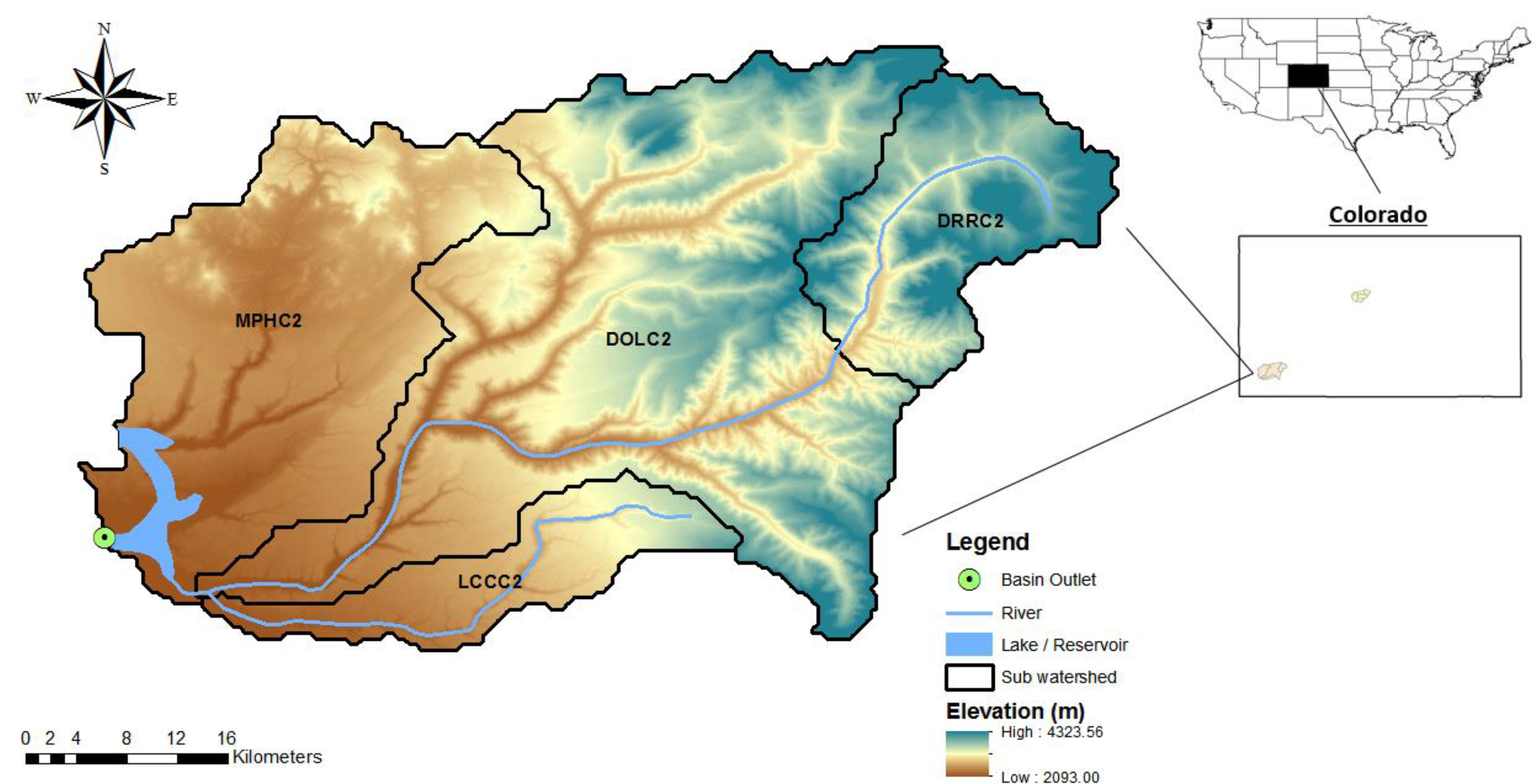
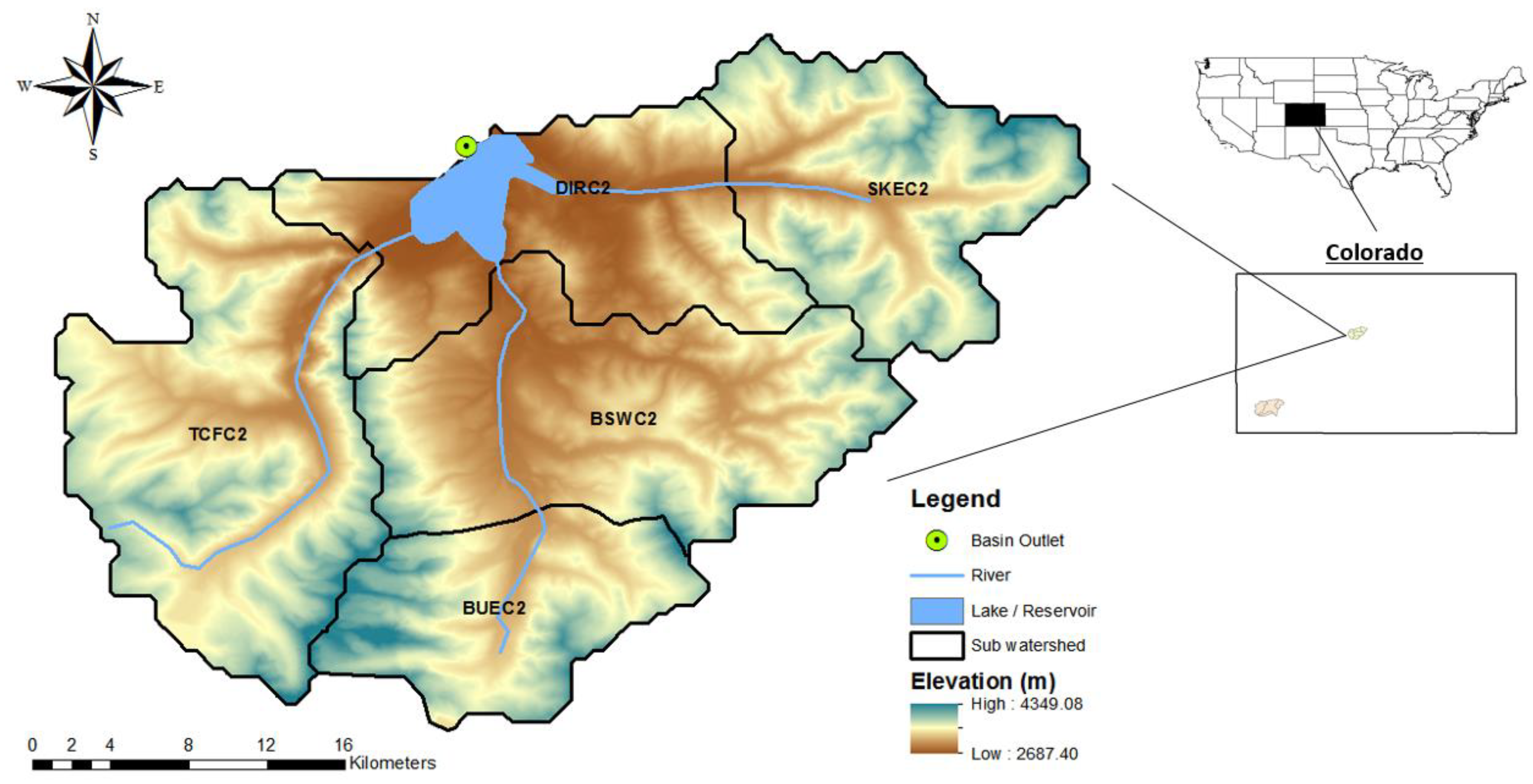
The study sites are within the Colorado River basin and include watersheds of the Dolores River above McPhee reservoir and the Blue River above Dillon reservoir (referred to as the Dolores River watershed and the Blue River watershed in the following sections) (Figure 1 and Figure 2). We chose these two study sites because (i) they represented different terrain and climate conditions, and (ii) they were high priority watersheds in the NASA-Roses project.
The average elevation of the Blue River watershed (3347 m) is higher than that of the Dolores River watershed (2786.54 m), whereas its total area (849.3 km2) is much smaller than that of the Dolores River watershed (2080.1 km2). Each site consists of head sub-watersheds and local sub-watersheds, with the details listed in Table 1. The annual mean temperature in the Dolores River watershed is slightly higher than that in the Blue River watershed (15.16 °C and 10.6 °C, respectively). The annual precipitation is around 700–750 mm in both watersheds. The major land types in both sites are evergreen and deciduous forests, as well as shrub, with the Dolores River watershed having a higher forest cover (87% and 53%, respectively).
We retrieved and processed data both from static datasets (e.g., topographic data and canopy cover data) and dynamic datasets (e.g., meteorological data) to prepare the model inputs. Precipitation and temperature are important model forcing inputs for both snow models. We utilized historical gridded precipitation and temperature datasets from the CBRFC. These 3-h time step, 800-m resolution datasets were created using the Mountain Mapper algorithm based on quality controlled climate station data [21]. We also used the CBRFC temperature data to derive the daily maximum and minimum temperature as inputs to the UEB model for radiation flux calculation. Wind speed and vapor pressure for the UEB model were prepared using gridded data from the NLDAS-2 land surface forcing dataset with 1/8th degree (around 13 km) grid spacing and an hourly time step [22].
Slope and aspect inputs for the UEB model were created using the 30-m National Elevation dataset (NED) [23], and canopy coverage fraction, canopy height, and leaf area index inputs for the UEB model were prepared using the 30-m National Land Cover dataset (NLCD) [24].
The RDHM framework uses the Hydrologic Rainfall Analysis Project (HRAP) grid system [25]. We defined the model resolution as 0.25 HRAP (around 1.2 km) and the model simulation time step as 6 hr. This choice was based on trading off computational considerations with explicit spatial detail. However, as UEB is a point model most meaningfully applied with a spatial footprint around 30 m [26], we applied UEB at grid cell centers within the 0.25 HRAP grid and with slope, aspect, and vegetation calculated from their respective 30-m scale datasets. This approach prevents the smoothing of the terrain that would occur if 1200-m grid cells were used but does not represent the variability of slope and aspect within any one grid cell. Rather, the assumption is that, aggregated over the watershed, these center points are sufficiently representative. Dynamic forcing data for the 1988–2010 time span were resampled from their 800-m (temperature and precipitation) or 1/8-degree (humidity and wind) resolution by selecting the value for the grid cell as the value where the 0.25 HRAP grid cell center falls.
The observed datasets used for performance evaluation included daily discharge and remotely sensed snow-covered area (SCA) data. Daily historical natural discharge data for 1988–2010 were obtained from the CBRFC, where they were produced by adjusting the USGS streamflow using diversion and reservoir data to calculate historical natural flows without the impacts of regulation. The MODIS Snow-Covered Area and Grain Size (MODSCAG) retrieval algorithm daily SCA data for 2000–2010 at 500-m resolution were used to evaluate the model snow outputs.
2.2. Models Description
We compared two model configurations for simulating snow and basin discharge, each of which coupled a snowmelt model with the SAC-SMA runoff model and the Rutpix7 routing model. The first configuration used the SNOW-17 temperature-index model, represented as SNOW-17+SAC-SMA+Rutpix7. The second used the UEB energy-balance model, represented as UEB+SAC-SMA+Rutpix7. The RDHM framework (with version 2.4.3) was used to support each of these model configurations. SNOW-17, SAC-SMA with a heat-transfer component (SAC-SMA-HT), and Rutpix7 models were already part of RDHM, whereas the UEB model was added to the framework as a new module in this research. This took advantage of the extensibility that RDHM provides for the addition of module code files configured following the developer’s instructions [27]. Descriptions of the two model configurations are provided in the following subsections.
2.2.1. Utah Energy Balance Model (UEB)
The UEB model is a physically based model for snow accumulation and melt developed to predict snowmelt rates that contribute to stream and river flows during the spring and summer. This model uses a single layer representation of the snowpack and a modified force restore approach [28,29] that allows the snow surface temperature to be different from the snow average temperature. This design avoids modeling the complex processes within a snowpack and provides a parsimonious model with a small number of state variables that is applicable over a spatial grid with no or minimal calibration at different locations. In addition, the UEB model’s vegetation component enhances its ability to model energy and mass balance processes in forested areas [30,31,32]. The vegetation component estimates the transmission and attenuation of radiation through a forest canopy, precipitation interception and unloading, snowmelt and sublimation of intercepted snow, and turbulent energy exchanges between the ground surface, canopy, and atmosphere.
The UEB model inputs include air temperature, precipitation, wind speed, relative humidity, incoming solar radiation, and longwave radiation at a time step sufficient to resolve the diurnal cycle (e.g., hourly, three-hourly, and six-hourly). Slope and aspect terrain conditions and canopy properties such as the leaf-area index, canopy height, and canopy cover are also required. In the absence of external input radiation, the solar and longwave radiation are parametrized using the air temperature, daily range of air temperature, and humidity. The daily temperature range is used to estimate the cloudiness fraction. The cloudiness fraction determines the direct and diffuse components of the solar radiation that reaches the surface of the earth and the emissivity of the atmosphere for longwave radiation. The equations and detailed description of the UEB radiation parametrization are provided in the model user manual [16].
In the UEB model, the two major state variables of energy content, U, and water equivalence, W, are determined at each time step using the inputs mentioned above and the following energy and mass balance equations.
In the energy-balance equation, the state variable U is energy per unit of horizontal area (kJ m−2). The flux terms are Qsn, net shortwave radiation; Qli, incoming longwave radiation; Qp, advected heat from precipitation; Qg, ground heat flux; Qle, outgoing longwave radiation; Qh, sensible heat flux; Qe, latent heat flux due to sublimation/condensation; and Qm, advected heat removed by meltwater, all of which are in units of energy per unit of horizontal area, per unit time (kJ m−2hr−1). In the mass-balance equation, the state variable W is the snow water equivalent (m). The flux terms are Pr, rainfall rate; Ps, snowfall rate; Mr, meltwater outflow from the snowpack; and Ε, sublimation from the snowpack, all in m/hr of water equivalent. Readers are referred to the UEB model papers [30,31,32] for details on how each process is modeled.
2.2.2. SNOW-17 Model
The SNOW-17 model is a conceptual model that uses precipitation as the water input and air temperature as the index to determine the energy exchange across the snow–air interface. This model is mainly used for river forecasting and requires the calibration of melt factors to generate reliable simulation results [4].
The SNOW-17 model calculates snow surface melt differently depending on whether rain is present or not. For rain on snow, the model computes the surface melt based on the following equation [4]:
where M is the depth of melt (mm); σ is the Stefan–Boltzmann constant; ∆t is the time interval (hr); Ta is the air temperature (°C); P is the water equivalent of precipitation (mm); fr is the fraction of precipitation in the form of rain; Tr is the rain temperature (°C); UADJ is the average wind function during rain-on-snow events (mm∙mb−1∙hr−1); ea is the vapor pressure of the air (mb); and Pa is the atmospheric pressure (mb). This calculation is based on energy-balance concepts but neglects solar radiation, assuming that the sky is overcast. The first term represents longwave radiation, the second represents melt by rain, and the third represents melt by sensible and latent heat. The parameter UADJ accounts for the effect of wind speed on the rate of snow melt through the turbulence flux of heat and water between the snow surface and the near-surface air layer. The initial value of UADJ is estimated from land cover type, which affects the wind profile near the surface as described in Koren et al. [33] and Anderson et al. [4].
When there is no rain and the air temperature is above the base value, the SNOW-17 model uses a melt factor to calculate the snowmelt as follows:
where M is the depth of melt (mm); Mf is a seasonally varying melt factor (mm/°C); Ta is the air temperature; Tb is the base temperature above which melt starts (usually 0 °C). To represent the seasonal variation in the melt factor, Mf is calculated from a sinusoidal curve with maximum (MFMAX) and minimum (MFMIN) melt factor values as model parameters [4].
The SNOW-17 model uses a heat deficit to keep track of the net heat loss from the snow cover under conditions of no surface melt [4]. When the air temperature is below freezing, the snow cover can lose or gain heat depending on the thermal gradient in the upper layers of the snowpack. This gradient is estimated as the difference between the snow surface temperature Tsur and the temperature at some distance within the snowpack computed as the antecedent temperature index (ATI). When Tsur is less than the ATI, the heat deficit is increasing; otherwise it is decreasing. When the heat deficit is zero and the amount of liquid water held in the pack equals the holding capacity, the snow cover is ripe and the excess liquid water will become the outflow. This is calculated using empirically derived equations to represent the lag and attenuation of water through the snow cover. Note that, unlike the UEB model, the SNOW-17 model does not have any representation of snow sublimation, and all snow water equivalent losses from SNOW-17 become snowmelt inputs to the SAC-SMA model of surface hydrology and runoff generation processes. For full details, refer to Anderson et al. [4].
2.2.3. Sacramento Soil Moisture Accounting Model (SAC-SMA)
The SAC-SMA model is a two-layer conceptual rainfall-runoff model [34]. This model parameterizes the soil characteristics that are responsible for streamflow production and represents soil moisture storage, percolation, drainage, and evapotranspiration (ET) processes in a conceptual way. It uses rain-plus-melt data as its input, which can be obtained from the output of snow models such as the SNOW-17 or the UEB model; however, it requires the calibration of parameters quantifying processes such as soil water storage and percolation rate to produce runoff simulations.
The SAC-SMA model estimates evapotranspiration (ET) using the available tension water volume and potential evaporation (PE) demand. When ET occurs, the moisture is withdrawn from the upper and lower zones of water tension. The PE demand is estimated using PE grids and PE adjustment factors. Twelve mean monthly PE grids are available for the model, and PE adjustment factors are used to account for the effects of vegetation.
2.2.4. Rutpix7
Rutpix7 is a hillslope and channel-routing model [17]. Inputs to the Rutpix7 model include fast (surface) and slow (subsurface/ground) runoff from the SAC-SMA model. In each cell, fast runoff is routed over a conceptual hillslope to a channel. Then, the channel inflow from the hillslopes, the slow runoff, and the upstream pixel outflows are routed through a cell conceptual channel, after which a topographically defined cell-to-cell connectivity sequence is used to move water from upstream to downstream. See Koren et al. [33] for details.
2.3. Model Calibration
We used code obtained from RTI International to automatically calibrate parameters for the snow and rainfall runoff models to minimize the difference between simulated and observed discharge. The code that RTI International provided implemented the Nondominated Sorting-based Multi-objective Genetic Algorithm II (NSGA-II) [35]. Three fitness functions were used in the algorithm: (i) Kling–Gupta efficiency [36] based on the difference between the simulated and observed discharge, (ii) the monthly volume difference between the observed and simulated discharge, and (iii) a penalty score to constrain model parameters within a prescribed valid range. To select a calibration parameter set on the pareto front defined by these metrics, the root-mean-square error (RMSE), Nash–Sutcliffe efficiency (NSE), and bias were evaluated for the simulated discharge and used to rank parameter sets from which the best, in the judgment of the author, was chosen. This automatic calibration was used to calibrate the SNOW-17 and the SAC-SMA model parameters given in Table 2. These parameters are either scalar, meaning that a single value applies to the whole domain, or gridded, meaning that they vary spatially. In the case of gridded parameters, RDHM provides procedures to compute a priori parameters based on topography, soils, and land cover information [17]. For our study watersheds, these a priori parameters were provided by RTI International. The spatial pattern from these geospatially derived a priori parameters was retained in the calibration algorithm by using a separate scalar multiplier for each grid parameter. Parameters (scalars and multipliers) were calibrated separately using the method described above for each sub-watershed using all the available data from 1988 to 2010.
In the first model configuration (SNOW-17+SAC-SMA+Rutpix7), the SNOW-17 and SAC-SMA model parameters were automatically calibrated. As a result of separate calibration for each sub-watershed, the scalar parameters such as the snow correction factor (SCF) and PE adjustment factors differ between sub-watersheds. In the second model configuration (UEB+SAC-SMA+Rutpix7), only SAC-SMA model parameters were automatically calibrated. The UEB model is physically based; thus, its parameters were held fixed at a priori published values and not calibrated. Initial results (not shown) revealed a low flow underestimation problem for some sub-watersheds that was diagnosed to be due to bias in the precipitation inputs. This bias occurred in the Blue River watershed and was indicated by the SNOW-17 SCF being larger than 1.2, which means the calibration adjusted the precipitation input multiplier to increase the precipitation input. The UEB model parameter that accounts for bias in precipitation input is the drift factor. In cases where SCF was larger than 1.2, we increased precipitation input by setting the drift factor to the SCF value. This was the only UEB parameter changed from a priori published values, and this change resolved the low flow underestimation problem.
Furthermore, Rutpix7 model parameters were kept constant using a set of pre-defined hillslope and channel parameters for both model configurations. RTI International completed the calibration for the first model configuration, and we calibrated the second model configuration.
2.4. Performance Measures
The MODSCAG SCA data product was used to compare simulated snow water equivalents from the two snow models. MODSCAG SCA data at ~500 m resolution were resampled using a nearest neighbor approach to 0.25 HRAP resolution and then classified as snow (value 1) where SCA was larger than 5% and as no snow (value 0) elsewhere. The modeled SWE was classified into a binary snow/no snow dataset using a 1-mm SWE threshold. The binary snow-cover maps were created only for the dates on which less than 10% of pixels were invalid (e.g., cloud cover or missing data) and at least one of the data sources (MODSCAG, UEB, SNOW-17) had snow in the watershed. Since there were insufficient valid observation data for the Blue River watershed, we focused comparison of the observed and simulated spatial distribution of the snowmelt process on the Dolores River watershed.
We used area and pixel-based methods to compare modeled and observed snow. The area-based comparison used fractional snow-covered area (Equation (5)) and calculated the mean absolute error (MAE) as the difference between the modeled and observed SCA fractions (Equation (6)). MAE calculations were performed separately for each month to account for seasonality and then averaged over all of the years with data. We also used the daily fractional SCA to calculate both the annual and melting period (March–June) NSE (Equation (7)). The pixel-based evaluation compared the observed and modeled binary snow-cover maps using a fitness statistic (Equation (8)) based on the number of pixels where snow was observed and modeled, observed and not modeled, not observed and modeled, and not observed and not modeled (Table 3) [37,38]. The fitness is the ratio between the number of pixels where both the simulation and observation have snow and the number of pixels where either the simulation or the observation has snow.
In these equations, Ns is the total number of pixels with snow in the binary snow-cover map; Nd is the total number of pixels without snow in the binary snow-cover map; fOi and fMi are the fractional SCA from observation and simulation; A, B, and C in the fitness function are the number of pixels in each group as defined in Table 3.
Basin discharge was simulated at a 6-hr time step and averaged as a daily time step for evaluation. Moreover, before using this result, we removed the first water year (water year 1989) as the system spin-up period. Observed daily discharge was compared with the simulation results using metrics of RMSE, NSE, bias, and percent April to July volume error:
where Oi and Mi are the daily discharge (m3s−1) from observation and simulation and VOi and VMi are the daily discharge volume (m3) of observation and simulation from April to July.
Aside from the snow and discharge analysis, we also compared the model outputs of sublimation and ET from the snow and runoff models to discover the differences between the two model configurations in simulating the evaporative components. We compared the water mass balance by calculating the simulated interannual domain average of precipitation, sublimation, and ET. We also examined the sublimation results of the UEB model in different land types to evaluate the model performance.
3. Results and Discussion
3.1. Snow Process Simulation
Both observation and simulation datasets for the Dolores River watershed were converted into binary snow-cover maps, and the evaluation metrics were calculated using results from 2000 to 2010. Table 4 shows the annual and melting period (March–June) NSE results. Table 5 shows the monthly MAE and fitness (except for July–September). The UEB model produced a higher NSE for both the annual and melting period and a lower MAE in most of the months compared to the SNOW-17 model, indicating that the UEB model performed better for the area-based evaluation. As for the fitness results, the SNOW-17 model had a higher fitness value most of the time, and hence a better pixel-based performance than the UEB model. Additionally, both models have higher fitness during the snow accumulation period (December–March) than during the melting (April–June) and early snowfall (October–November) periods. This is because both observation and simulation have a high SCA over the watershed during the snow accumulation period, which increases the possibility of matching pixels between the simulation and observation binary snow-cover maps.
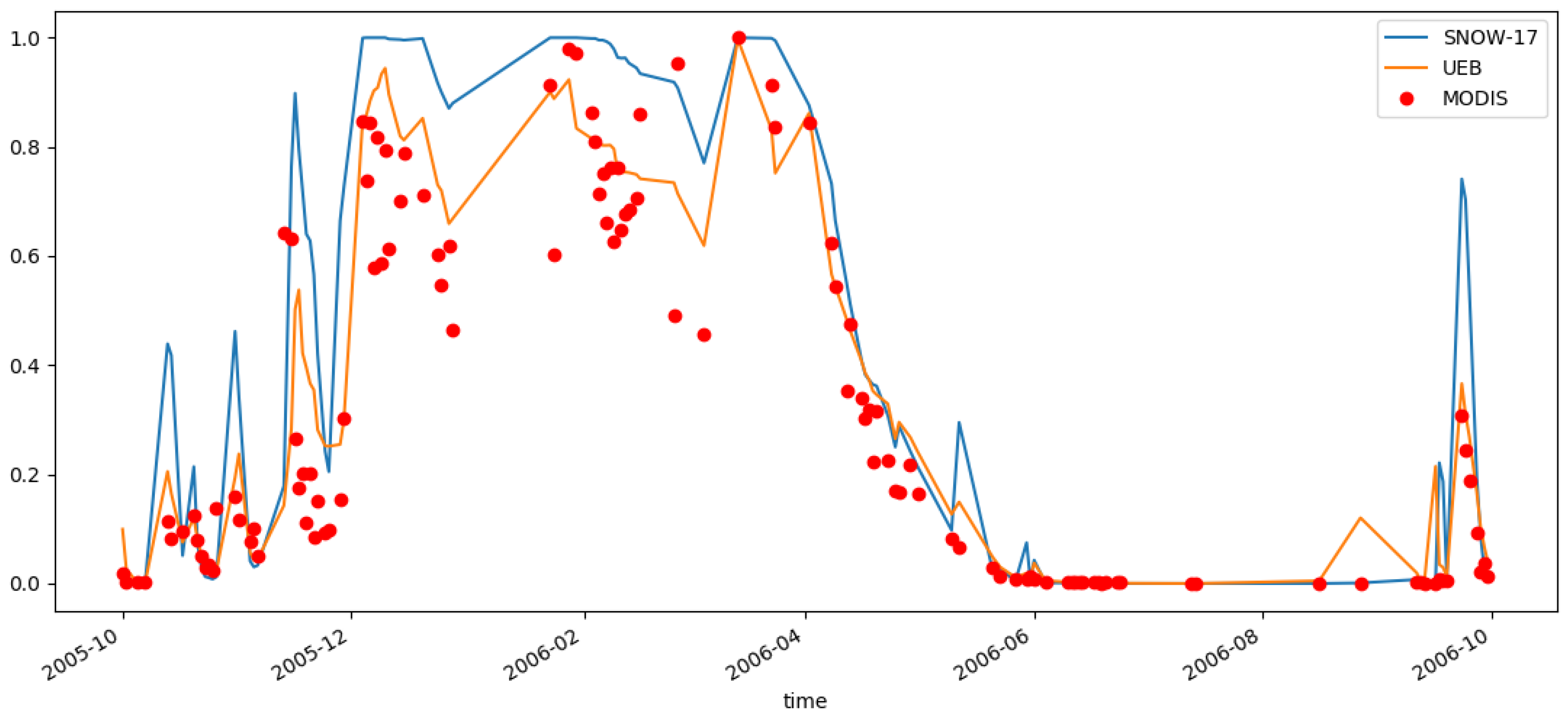
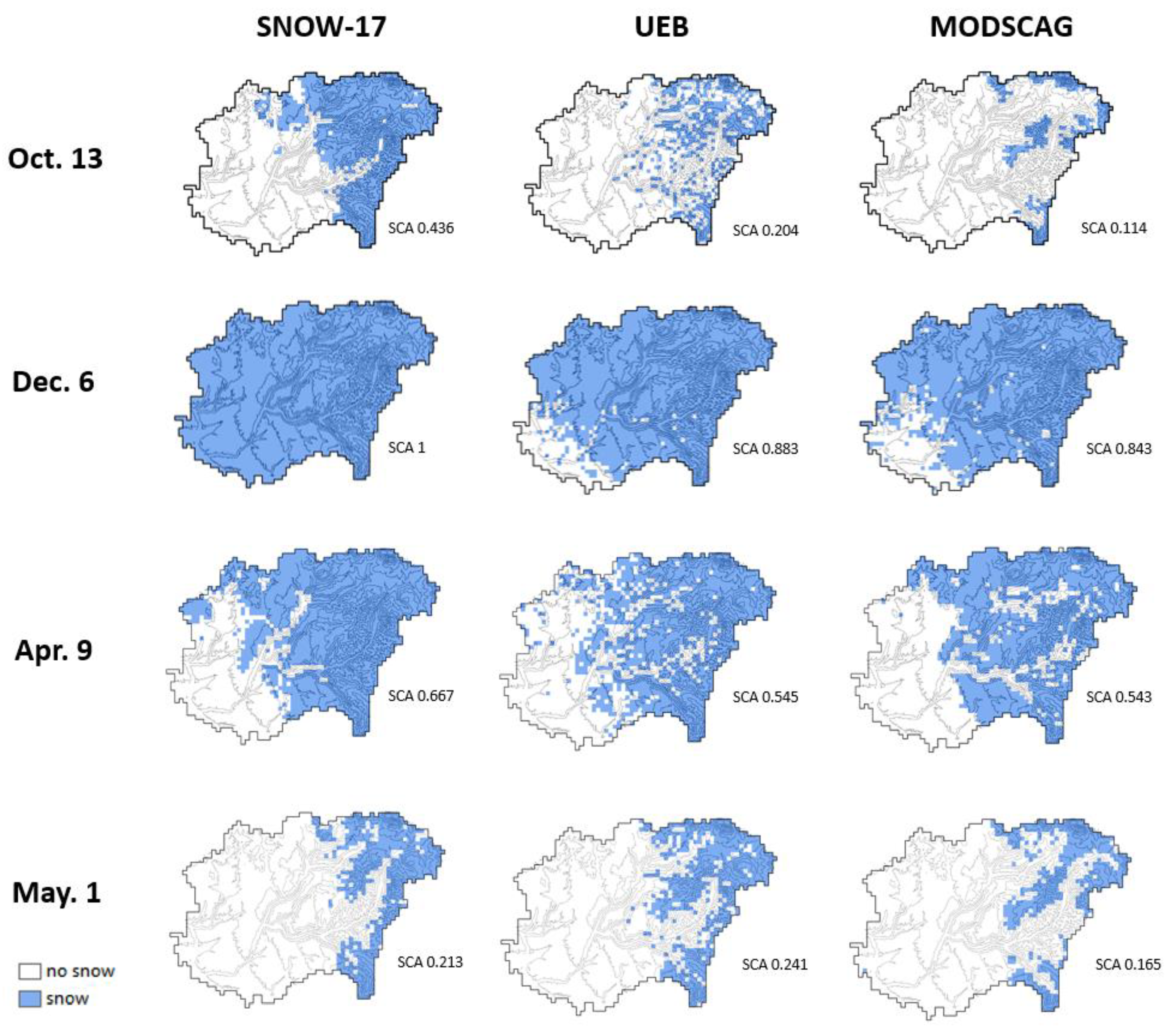
In order to gain a better understanding of the spatial and temporal dynamics of the SCA in the watershed, we further examined the results in water year 2006, which has the largest number of satellite observation images with sufficient valid data. A time-series plot of the modeled and observed fractional SCA during water year 2006 (Figure 3), shows that both models generally follow the observed SCA pattern. During the snow accumulation period, the SNOW-17 model tended to have higher peaks (e.g., during October and November) and overestimate the SCA more than the UEB model does. During the melting period, both models simulated the snowmelt process with reasonable timing and amount compared to the observational data. The binary snow-cover maps (Figure 4) show the spatial distribution of snow cover from the two snow models and the MODSCAG observations for various dates in water year 2006. The four days correspond to the accumulation (13 October, 6 December) and snowmelt (9 April, 1 May) periods. The maps show that the UEB model better captures the reduction in area during melt-out, whereas the SNOW-17 model overestimates the SCA. This is also a problem during the snow accumulation period (13 October). Examining the UEB SCA simulations, a scattered or pixelated pattern is present (e.g., 13 October). This is due to the UEB model using terrain parameters (slope and aspect) at the center point of each 0.25 HRAP grid cell. These center point values do not represent the larger grid cell as a whole and may have slope and aspect disassociated with the slope and aspect of adjacent large grid cell centers, leading to the pixelated SCA pattern.
The UEB model’s better performance in the area-based evaluation can be explained as follows. First, the automatic-calibration adjusted SCF (SCF > 1) from the SNOW-17 model leads to greater snow accumulation, which may delay snow disappearance. Second, the UEB model does simulate sublimation, which may lead to more rapid snow depletion and disappearance than SNOW-17. Third, the SNOW-17 model uses a melt factor to implicitly represent the energy input and corresponding topographic effect for snowmelt, whereas the UEB model directly calculates the radiation fluxes using slope, aspect, and canopy data as inputs. This makes the UEB model more sensitive to the variability in melting caused by different terrain conditions.
For pixel-based evaluation, the UEB model uses the slope and aspect at the center point of each pixel to represent the terrain features of the corresponding grid area. However, terrain features at the center points are different from the grid cell as a whole, especially when the grid spacing is large, and this may lead to the mismatch with observed SCA and thus a lower fitness. However, the similarity of the aggregate observed and UEB SCA suggests that over the basin these points may be sufficient to represent basin terrain variability, something that is not achieved by SNOW-17 which does not account for slope and aspect.
3.2. Basin Discharge Simulation
We evaluated the basin discharge performance by comparing the observed and simulated daily discharge with different evaluation metrics for water years 1990–2010. According to the values of the different performance metrics, the overall model performance for the basin discharge simulation indicated a satisfactory calibration for each model configuration in the two watersheds (Table 6 and Table 7). In the Dolores River watershed, the UEB model had a somewhat better performance than the SNOW-17 model, with a higher NSE and lower values for the other metrics in most of the sub-watersheds, whereas the SNOW-17 model outperforms the UEB model somewhat in the Blue River watershed when comparing these metrics. In addition, the head watershed LCCC2 had a much lower NSE, indicating that the model performance was not as good as for the other sub-watersheds. This is because LCCC2 has much less precipitation input than other sub-watersheds and generates intermittent streamflow that mainly happens during the spring melt season, with almost no streamflow during July to September. Since neither snow model can simulate the streamflow during dry periods well (results not shown here), the model performance for this sub-watershed is not as good as for the others.
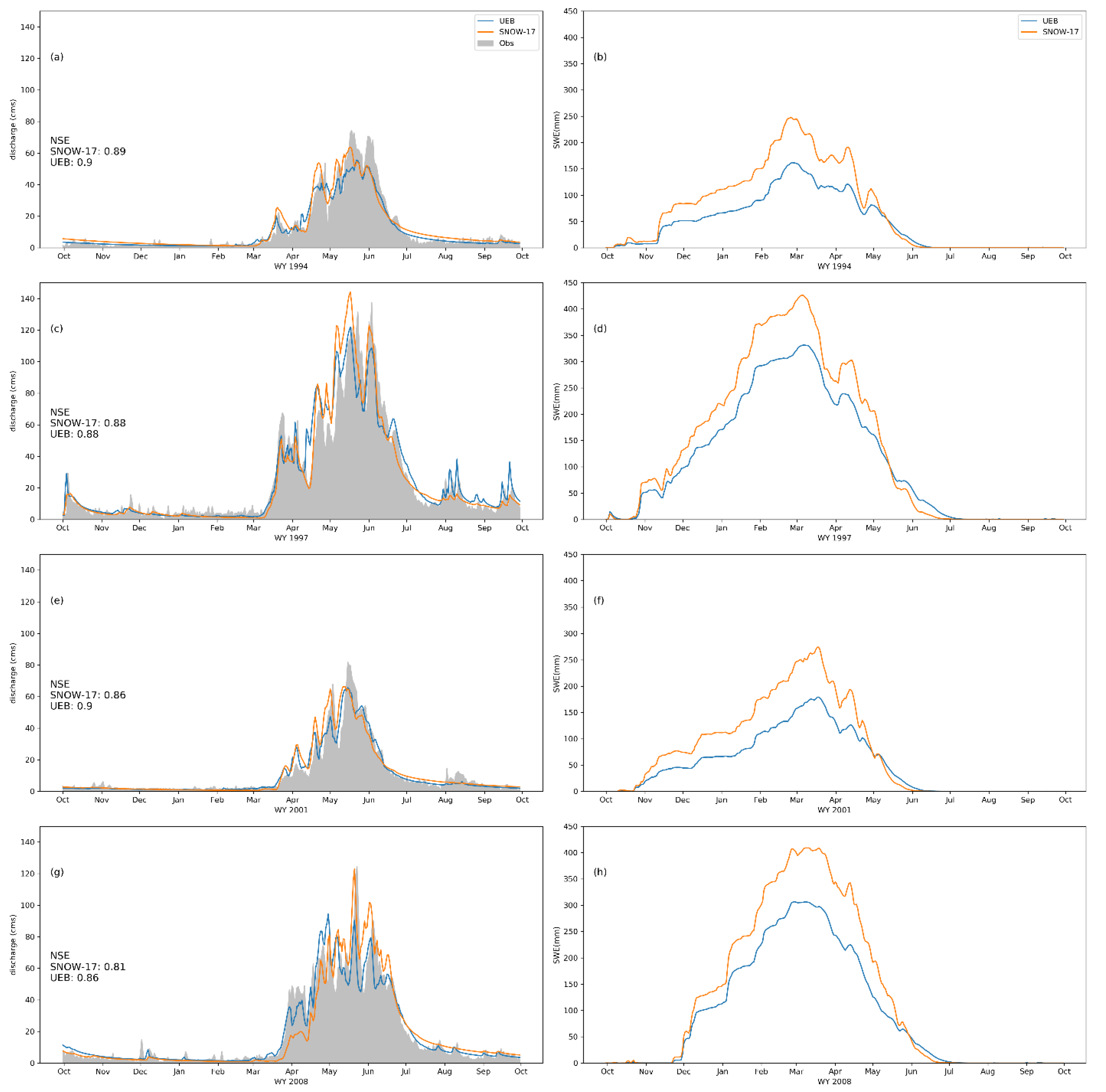
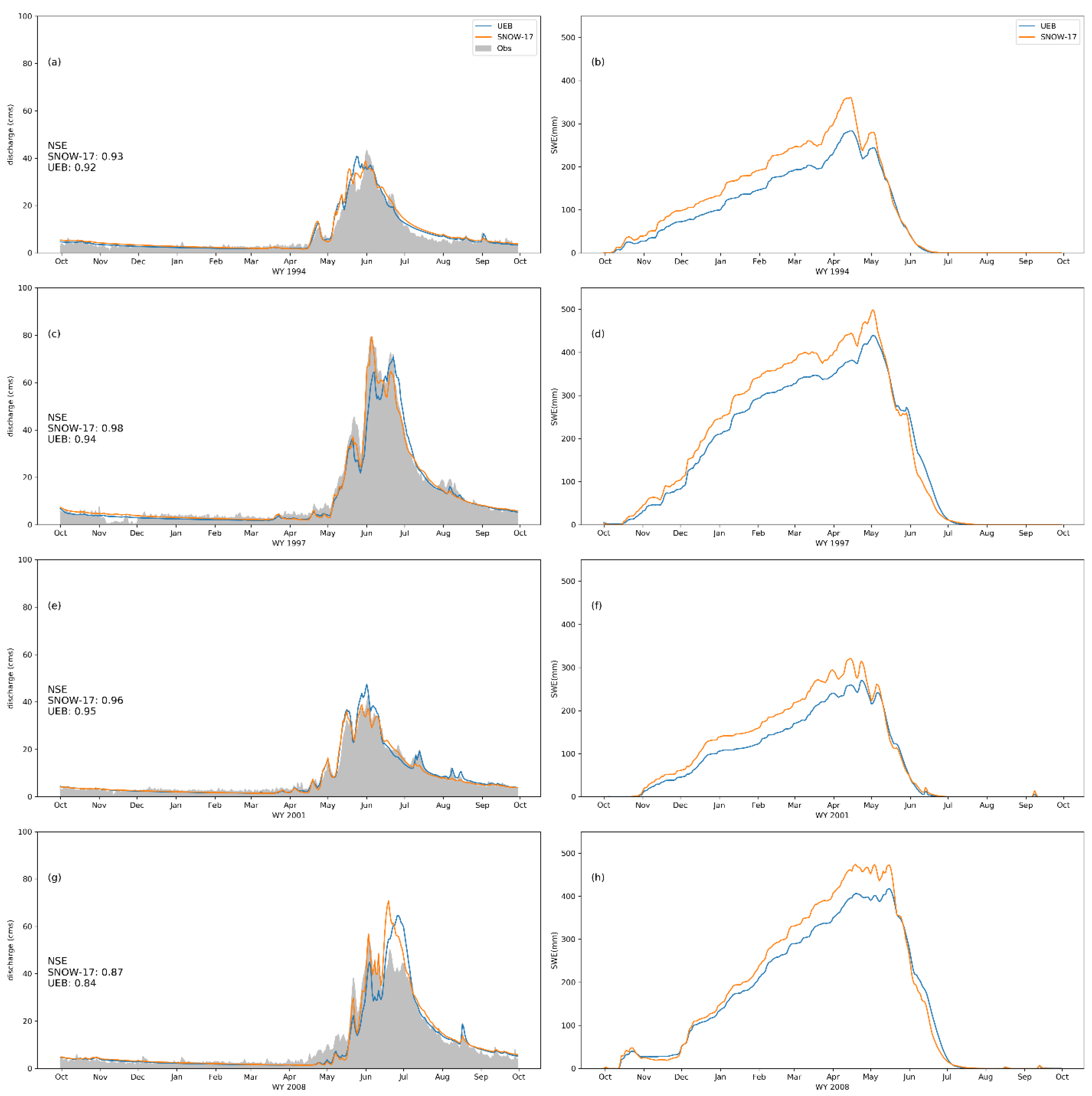
Figure 5 and Figure 6 present the simulated domain average SWE and observed and simulated discharge in different water years (1994, 1997, 2001, and 2008) for the Dolores River and Blue River watersheds, respectively. These years were chosen because they were typical of and spanned the range of model performance over the two decades (22 years), except for one year that was exceptionally dry and where there was a poor model performance from both models (water year 2002). These results show that the two snow models coupled to SAC-SMA and Rutpix7 provide reasonable discharge simulations for the two watersheds, each of which had different snowmelt and discharge patterns.
Aside from the discharge results, both the SNOW-17 and the UEB model were found to have similar timing for snow accumulation and snowmelt. The SNOW-17 model has a higher SWE during the accumulation period mainly because the UEB model simulates water loss from sublimation, leading to less snow accumulation than the SNOW-17 model. As a result, the SNOW-17 model actually provides more rain-plus-melt input to feed the SAC-SMA model that simulates the runoff and ET processes. This leads to differences in the simulated quantity of ET from the two model configurations. This will be discussed in the next subsection.
3.3. Evaporative Components Simulation
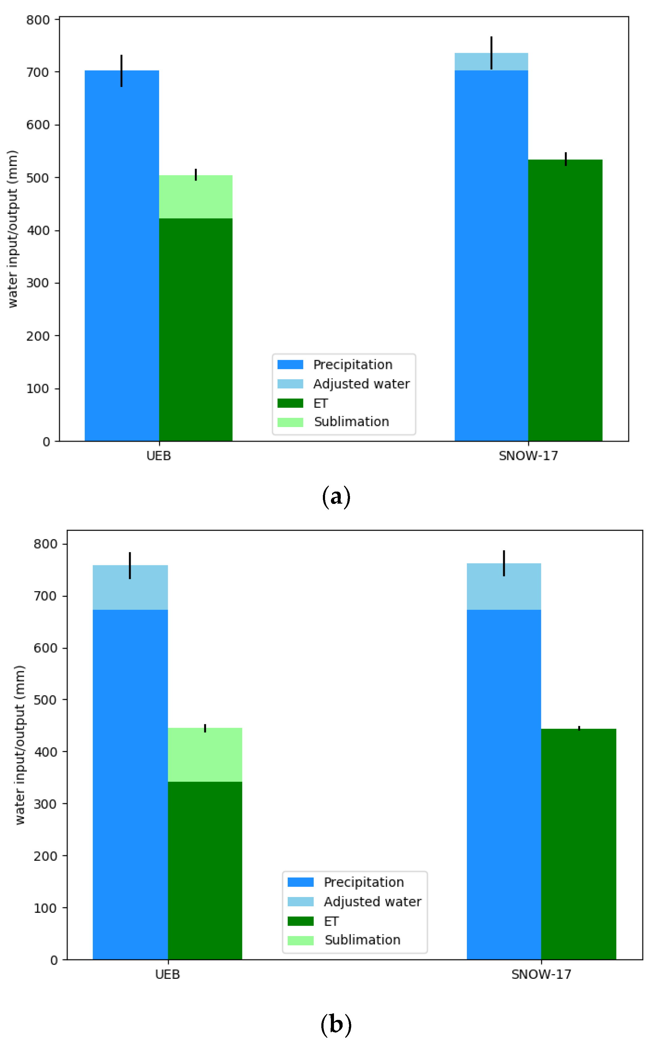
The UEB model coupled to SAC-SMA simulates both sublimation and ET. However, since SNOW-17 does not simulate sublimation, the only evaporative component in the SNOW-17 model coupled to SAC-SMA is ET. In order to better understand the consequences of this difference, we compared the water mass balance from the two model configurations. We calculated the watershed average of annual mean precipitation, sublimation, and ET for the two watersheds over the simulation period (Figure 7). Precipitation adjustments made to SNOW-17 through the SCF parameter, and to UEB through the drift factor parameter, are shown. Precipitation inputs to both snowmelt models were adjusted by a similar amount in the Blue River watershed, whereas only the SNOW-17 model was adjusted in the Dolores River watershed, noting from the calibration section above that the drift factor was not adjusted when the SCF was less than 1.2. Since the simulated precipitation inputs are similar and the models were calibrated against the same observed discharge, both model configurations have similar total evaporative components for each of the watersheds. The UEB model, however, explicitly simulated the portion due to sublimation. The results show that the water loss due to sublimation is a considerable amount (12–13% of annual mean precipitation), and it should not be neglected in the snow mass balance for these watersheds.
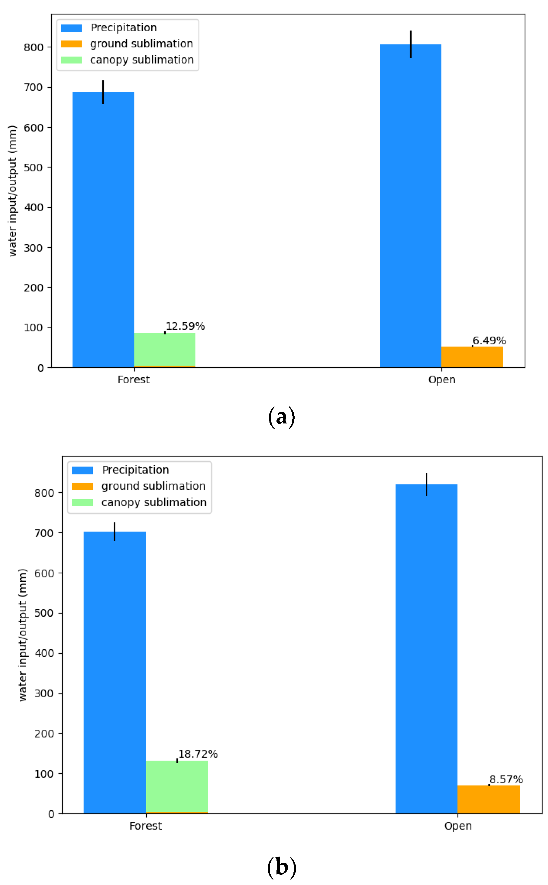
We further examined the canopy and ground sublimation simulated by the UEB model for different land types (Figure 8). This figure shows the watershed average of the annual mean precipitation, as well as the canopy and ground sublimation for forest and open areas. The canopy sublimation in the forest area dominates the process, and the total water loss from sublimation in the forest areas is about twice as much as in the open area. In addition, the annual mean precipitation and canopy sublimation were compared for different forest types and at different elevations using the simulated results at each grid cell over the watershed domain. Figure 9 shows that annual precipitation increases with increased elevation, and the canopy sublimation increases with increased elevation, precipitation, and forest density, determined by the LAI, canopy cover, and canopy height of different forest types (Table 8). These results are similar to findings from other works that have evaluated sublimation variability in semi-arid mountainous regions [39,40]. For the sensitivity analysis of the UEB model for various canopy types, please refer to the previous work by Mahat et al. [32].
Since a large fraction of both watersheds consists of forest area (87% in the Dolores River watershed and 53% in the Blue River watershed), land type changes may affect sublimation and thus impact the water mass balance in the watersheds [41,42,43]. This analysis highlights the advantages of using the UEB model, including it better quantifying the proportions of the different evaporative components and providing the means to evaluate the impact of land cover change on the sublimation process and the corresponding influence on water availability in the watershed. Using SNOW-17 to accomplish these same tasks would be difficult or impossible because the model does not directly account for the sublimation process.
4. Summary and Conclusions
This research is part of a project with the objective to assess whether applying an energy-balance model in the river forecasting system used by CBRFC would improve water supply forecasts in the Colorado River basin. This research focused on using analysis of historical, or retrospective, model simulations to evaluate model performance in comparison to snow-covered area, daily discharge, and water mass balance. The UEB and SNOW-17 models were evaluated by coupling them with the SAC-SMA model and the Rutpix7 model within the RDHM framework for distributed modeling of basin snow and discharge in the Dolores and Blue River watersheds. Parameters for the SNOW-17 and the SAC-SMA models were calibrated using an automated multi-objective procedure. In the UEB model, the drift factor parameter was adjusted to account for the precipitation input bias, but other parameters were held fixed at their literature values.
Comparison of the simulated and observed SCA data showed that both snow models were able to simulate the spatial and temporal change in the SCA in the Dolores River watershed with reasonable timing and amount (e.g., the annual NSE of SCA is larger than 0.7). The results indicated that both model configurations were also able to provide good discharge simulation results for the study sites (e.g., the NSE of discharge is between 0.85 and 0.94 for most sub-watersheds). Although both models have a similar performance, the UEB model showed its potential for application in the river forecasting system to advance water supply forecasts for future changing conditions. First, the UEB model was able to simulate the sublimation process for different land cover types, whereas sublimation is not represented in the SNOW-17 model. Sublimation is an important evaporative component during the snow season in the Colorado River basin, and the UEB model demonstrated its capability to evaluate sublimation water loss and its impact on the water mass balance when the land type alters. Second, the UEB model held parameters (except for the drift factor) constant and achieved fit metrics comparable to the SNOW-17 model, where parameters were calibrated for each sub-watershed. This suggests that the UEB model parameters are more transferable and provide the ability to simulate the snowmelt process under different terrain or climate conditions, thus reducing the intensive model calibration work required within the temperature-index model to provide a reliable simulation. Moreover, the maximum/minimum melt factors in the SNOW-17 model were calibrated against historical data, which may not well represent the melt rate under potential future conditions given a changing climate. In contrast, the UEB model accounts for the physical process of snowmelt based on energy and water mass balance, which means it is more capable of providing reliable predictions when climate patterns change. However, the performance of the UEB model was found to be affected by biases in the input precipitation. It was necessary to adjust the UEB model’s drift factor based on the SNOW-17 model’s SCF values to resolve low flow underestimation caused by the precipitation input bias in the Blue River watershed. Without the reference SCF value, it may be challenging to estimate the data bias and calibrate the UEB model parameters, demanding more simulation time and computing resources than the SNOW-17 model for automatic calibration.
Additional work would help further understand the UEB model performance for operational water supply forecasts. One direction is to conduct model validation with the two model configurations and evaluate their performances. In this research, we utilized all the available historical datasets for model calibration to achieve reliable simulation results. This is an initial exploration of the feasibility of applying the UEB model in the RDHM framework and the proposed direction will provide more insights into the UEB model’s performance. Another direction is to evaluate model performance when running the UEB model at higher spatial resolutions. It is assumed that the energy-balance model will provide a better performance at finer resolution because of the better representation of the spatial variation in topographic and vegetation features. However, a higher model resolution will require more computing resources and a longer simulation time. Balancing the trade-offs between model performance and the computational demand of model operation is an important issue for operational water supply forecasts.
Author Contributions
Conceptualization, T.G., D.G.T. and T.Z.G.; methodology, T.G. and D.G.T.; software, T.G. and T.Z.G.; validation, T.G.; formal analysis, T.G.; investigation, T.G.; resources, T.G.; data curation, T.G.; writing—original draft preparation, T.G.; writing—review and editing, T.G., D.G.T. and T.Z.G.; visualization, T.G.; supervision, D.G.T.; project administration, D.G.T.; funding acquisition, D.G.T. All authors have read and agreed to the published version of the manuscript.
Funding
This work was supported by the NASA award NNH15CM90C.
Data Availability Statement
The National Elevation dataset can be found at https://earthexplorer.usgs.gov/ (accessed on 1 March 2023). The National Land Cover dataset can be found at https://www.mrlc.gov/data (accessed on 1 March 2023). The NLDAS-2 land surface data can be found at https://disc.gsfc.nasa.gov/datasets (accessed on 1 March 2023). The temperature, precipitation, historical natural discharge dataset, and the MODIS snow-covered area and grain size dataset are available on request from the Colorado Basin River Forecast Center.
Acknowledgments
This work was supported by NASA award NNH15CM90C. Any opinions, findings, and conclusions or recommendations expressed in this material are those of the authors and do not necessarily reflect the views of NASA. We are also thankful to collaborators from RTI International for providing research datasets, model parameters, model calibration code, and results for the SNOW17+SAC-SMA+Rutpix7 model configuration to support this research.
Conflicts of Interest
The authors declare that they have no known competing financial interests or personal relationships that could have appeared to influence the work reported in this paper.
References
- Li, D.; Wrzesien, M.L.; Durand, M.; Adam, J.; Lettenmaier, D.P. How Much Runoff Originates as Snow in the Western United States, and How Will That Change in the Future? Geophys. Res. Lett. 2017, 44, 6163–6172. [Google Scholar] [CrossRef]
- Anderson, E.A. National Weather Service River Forecast System: Snow Accumulation and Ablation Model; US National Weather Service: Silver Spring, MD, USA, 1973. Available online: https://repository.library.noaa.gov/view/noaa/13507/noaa_13507_DS1.pdf (accessed on 1 March 2023).
- Burnash, R.J.C.; Ferral, R.L.; McGuire, R.A. A Generalized Streamflow Simulation System: Conceptual Modeling for Digital Computers; U.S. Department of Commerce National Weather Service: Silver Spring, MD, USA; State of California Department of Water Resources: Sacramento, CA, USA, 1973.
- Anderson, E.A. Snow Accumulation and Ablation Model–SNOW-17; US National Weather Service: Silver Spring, MD, USA, 2006. Available online: https://www.weather.gov/media/owp/oh/hrl/docs/22snow17.pdf (accessed on 1 March 2023).
- Hock, R. Temperature Index Melt Modelling in Mountain Areas. J. Hydrol. 2003, 282, 104–115. [Google Scholar] [CrossRef]
- Zierl, B.; Bugmann, H. Global Change Impacts on Hydrological Processes in Alpine Catchments. Water Resour. Res. 2005, 41, W02028. [Google Scholar] [CrossRef]
- Barnett, T.P.; Adam, J.C.; Lettenmaier, D.P. Potential Impacts of a Warming Climate on Water Availability in Snow-Dominated Regions. Nature 2005, 438, 303–309. [Google Scholar] [CrossRef]
- Sturm, M.; Goldstein, M.A.; Parr, C. Water and Life from Snow: A Trillion Dollar Science Question. Water Resour. Res. 2017, 53, 3534–3544. [Google Scholar] [CrossRef]
- Zeinivand, H.; De Smedt, F. Hydrological Modeling of Snow Accumulation and Melting on River Basin Scale. Water Resour. Manag. 2009, 23, 2271–2287. [Google Scholar] [CrossRef]
- Essery, R.; Morin, S.; Lejeune, Y.; Ménard, C.B. A Comparison of 1701 Snow Models Using Observations from an Alpine Site. Adv. Water Resour. 2013, 55, 131–148. [Google Scholar] [CrossRef]
- Magnusson, J.; Wever, N.; Essery, R.; Helbig, N.; Winstral, A.; Jonas, T. Evaluating Snow Models with Varying Process Representations for Hydrological Applications. Water Resour. Res. 2015, 51, 2707–2723. [Google Scholar] [CrossRef]
- Shakoor, A.; Burri, A.; Bavay, M.; Ejaz, N.; Razzaq Ghumman, A.; Comola, F.; Lehning, M. Hydrological Response of Two High Altitude Swiss Catchments to Energy Balance and Temperature Index Melt Schemes. Polar Sci. 2018, 17, 1–12. [Google Scholar] [CrossRef]
- Franz, K.J.; Hogue, T.S.; Sorooshian, S. Operational Snow Modeling: Addressing the Challenges of an Energy Balance Model for National Weather Service Forecasts. J. Hydrol. 2008, 360, 48–66. [Google Scholar] [CrossRef]
- Debele, B.; Srinivasan, R.; Gosain, A.K. Comparison of Process-Based and Temperature-Index Snowmelt Modeling in SWAT. Water Resour. Manag. 2010, 24, 1065–1088. [Google Scholar] [CrossRef]
- Kumar, M.; Marks, D.; Dozier, J.; Reba, M.; Winstral, A. Evaluation of Distributed Hydrologic Impacts of Temperature-Index and Energy-Based Snow Models. Adv. Water Resour. 2013, 56, 77–89. [Google Scholar] [CrossRef]
- Tarboton, D.G.; Luce, C.H. Utah Energy Balance Snow Accumulation and Melt Model (UEB). In Computer Model Technical Description and Users Guide; Utah Water Research Laboratory: Logan, UT, USA; USDA Forest Service Intermountain Research Station: Ogden, UT, USA, 1996. [Google Scholar]
- NWS. Hydrology Laboratory-Research Distributed Hydrologic Model (HL-RDHM) User Manual V. 3.0.0. Available online: https://www.cbrfc.noaa.gov/present/rdhm/RDHM_3_0_0_User_Manual.pdf (accessed on 1 March 2023).
- Painter, T.H.; Rittger, K.; McKenzie, C.; Slaughter, P.; Davis, R.E.; Dozier, J. Retrieval of Subpixel Snow Covered Area, Grain Size, and Albedo from MODIS. Remote Sens. Environ. 2009, 113, 868–879. [Google Scholar] [CrossRef]
- Micheletty, P.; Perrot, D.; Day, G.; Rittger, K. Assimilation of Ground and Satellite Snow Observations in a Distributed Hydrologic Model for Water Supply Forecasting. JAWRA J. Am. Water Resour. Assoc. 2022, 58, 1030–1048. [Google Scholar] [CrossRef]
- Gichamo, T.Z.; Tarboton, D.G. Ensemble Streamflow Forecasting Using an Energy Balance Snowmelt Model Coupled to a Distributed Hydrologic Model with Assimilation of Snow and Streamflow Observations. Water Resour. Res. 2019, 55, 10813–10838. [Google Scholar] [CrossRef]
- Schaake, J.; Henkel, A.; Cong, S. Application of Prism Climatologies for Hydrologic Modeling and Forcasting in the Western U.S. In Proceedings of the 18th Conference on Hydrology, Seattle, WA, USA, 12–15 January 2004; Available online: https://ams.confex.com/ams/pdfpapers/72159.pdf (accessed on 1 March 2023).
- Xia, Y.; Mitchell, K.; Ek, M.; Sheffield, J.; Cosgrove, B.; Wood, E.; Luo, L.; Alonge, C.; Wei, H.; Meng, J.; et al. Continental-Scale Water and Energy Flux Analysis and Validation for the North American Land Data Assimilation System Project Phase 2 (NLDAS-2): 1. Intercomparison and Application of Model Products. J. Geophys. Res. Atmos. 2012, 117, D03109. [Google Scholar] [CrossRef]
- Gesch, D.B. The National Elevation Dataset. In Digital Elevation Model Technologies and Applications—The DEM Users Manual; Maune, D., Ed.; American Society for Photogrammetry and Remote Sensing: Bethesda, MD, USA, 2007; pp. 99–118. [Google Scholar]
- Homer, C.; Dewitz, J.; Yang, L.; Jin, S.; Danielson, P.; Xian, G.; Coulston, J.; Herold, N.; Wickham, J.; Megown, K. Completion of the 2011 National Land Cover Database for the Conterminous United States–Representing a Decade of Land Cover Change Information. Photogramm. Eng. Remote Sens. 2015, 81, 345–354. [Google Scholar]
- Reed, S.M.; Maidment, D.R. Coordinate Transformations for Using NEXRAD Data in GIS-Based Hydrologic Modeling. J. Hydrol. Eng. 1999, 4, 174–182. [Google Scholar] [CrossRef]
- Tarboton, D.G.; Blöschl, G.; Cooley, K.; Kirnbauer, R.; Luce, C. Spatial Snow Cover Processes at Kühtai and Reynolds Creek. In Spatial Patterns in Catchment Hydrology: Observations and Modelling; Grayson, R., Blöschl, G., Eds.; Cambridge University Press: Cambridge, UK, 2000; pp. 158–186. [Google Scholar]
- NWS. The HL Research Distributed Hydrologic Model (HL-RDHM) Developer’s Manual v. 2.0. Available online: https://www.cbrfc.noaa.gov/present/rdhm/rdhm_developers_manual.pdf (accessed on 1 March 2023).
- Luce, C.; Tarboton, D.G. A Modified Force-Restore Approach to Modeling Snow-Surface Heat Fluxes. In Proceedings of the 69th Annual Western Snow Conference, Sun Valley, ID, USA, 16–19 April 2001. [Google Scholar]
- Luce, C.; Tarboton, D.G. Evaluation of Alternative Formulae for Calculation of Surface Temperature in Snowmelt Models Using Frequency Analysis of Temperature Observations. Hydrol. Earth Syst. Sci. 2010, 14, 535–543. [Google Scholar] [CrossRef]
- Mahat, V.; Tarboton, D.G. Canopy Radiation Transmission for an Energy Balance Snowmelt Model. Water Resour. Res. 2012, 48, W01534. [Google Scholar] [CrossRef]
- Mahat, V.; Tarboton, D.G.; Molotch, N.P. Testing Above- and below-Canopy Representations of Turbulent Fluxes in an Energy Balance Snowmelt Model. Water Resour. Res. 2013, 49, 1107–1122. [Google Scholar] [CrossRef]
- Mahat, V.; Tarboton, D.G. Representation of Canopy Snow Interception, Unloading and Melt in a Parsimonious Snowmelt Model. Hydrol. Process 2014, 28, 6320–6336. [Google Scholar] [CrossRef]
- Koren, V.; Reed, S.; Smith, M.; Zhang, Z.; Seo, D.J. Hydrology Laboratory Research Modeling System (HL-RMS) of the US National Weather Service. J. Hydrol. 2004, 291, 297–318. [Google Scholar] [CrossRef]
- NWS. Conceptualization of the Sacramento Soil Moisture Accounting Model. Available online: https://www.nws.noaa.gov/oh/hrl/nwsrfs/users_manual/part2/_pdf/23sacsma.pdf (accessed on 1 March 2019).
- Deb, K.; Pratap, A.; Agarwal, S.; Meyarivan, T. A Fast and Elitist Multiobjective Genetic Algorithm: NSGA-II. IEEE Trans. Evol. Comput. 2002, 6, 182–197. [Google Scholar] [CrossRef]
- Gupta, H.V.; Kling, H.; Yilmaz, K.K.; Martinez, G.F. Decomposition of the Mean Squared Error and NSE Performance Criteria: Implications for Improving Hydrological Modelling. J. Hydrol. 2009, 377, 80–91. [Google Scholar] [CrossRef]
- Aronica, G.; Bates, P.D.; Horritt, M.S. Assessing the Uncertainty in Distributed Model Predictions Using Observed Binary Pattern Information within GLUE. Hydrol. Process 2002, 16, 2001–2016. [Google Scholar] [CrossRef]
- Bernhardt, M.; Schulz, K. SnowSlide: A Simple Routine for Calculating Gravitational Snow Transport. Geophys. Res. Lett. 2010, 37, L11502. [Google Scholar] [CrossRef]
- Sexstone, G.A.; Clow, D.W.; Fassnacht, S.R.; Liston, G.E.; Hiemstra, C.A.; Knowles, J.F.; Penn, C.A. Snow Sublimation in Mountain Environments and Its Sensitivity to Forest Disturbance and Climate Warming. Water Resour. Res. 2018, 54, 1191–1211. [Google Scholar] [CrossRef]
- Montesi, J.; Elder, K.; Schmidt, R.A.; Davis, R.E. Sublimation of Intercepted Snow within a Subalpine Forest Canopy at Two Elevations. J. Hydrometeorol. 2004, 5, 763–773. [Google Scholar] [CrossRef]
- Penn, C.A.; Bearup, L.A.; Maxwell, R.M.; Clow, D.W. Numerical Experiments to Explain Multiscale Hydrological Responses to Mountain Pine Beetle Tree Mortality in a Headwater Watershed. Water Resour. Res. 2016, 52, 3143–3161. [Google Scholar] [CrossRef]
- Biederman, J.A.; Brooks, P.D.; Harpold, A.A.; Gochis, D.J.; Gutmann, E.; Reed, D.E.; Pendall, E.; Ewers, B.E. Multiscale Observations of Snow Accumulation and Peak Snowpack Following Widespread, Insect-Induced Lodgepole Pine Mortality. Ecohydrology 2014, 7, 150–162. [Google Scholar] [CrossRef]
- Harpold, A.A.; Biederman, J.A.; Condon, K.; Merino, M.; Korgaonkar, Y.; Nan, T.; Sloat, L.L.; Ross, M.; Brooks, P.D. Changes in Snow Accumulation and Ablation Following the Las Conchas Forest Fire, New Mexico, USA. Ecohydrology 2014, 7, 440–452. [Google Scholar] [CrossRef]
Figure 1.
Dolores River above McPhee Reservoir study site.

Figure 2.
Blue River above Dillon Reservoir study site.

Figure 3.
Modeled and observed MODIS fractional SCA in water year 2006 in the Dolores River watershed.
Figure 3.
Modeled and observed MODIS fractional SCA in water year 2006 in the Dolores River watershed.

Figure 4.
Snow cover maps for model simulations and MODIS observation at different dates in water year 2006 in the Dolores River watershed.
Figure 4.
Snow cover maps for model simulations and MODIS observation at different dates in water year 2006 in the Dolores River watershed.

Figure 5.
Simulated and observed daily discharge (left) and simulated domain average SWE (right) in the Dolores River watershed for four water years (WY). Panel (a,b) are results for water year 1994; panel (c,d) for water year 1997; panel (e,f) for water year 2001; panel (g,h) for water year 2008.
Figure 5.
Simulated and observed daily discharge (left) and simulated domain average SWE (right) in the Dolores River watershed for four water years (WY). Panel (a,b) are results for water year 1994; panel (c,d) for water year 1997; panel (e,f) for water year 2001; panel (g,h) for water year 2008.

Figure 6.
Simulated and observed daily discharge (left) and simulated domain average SWE (right) in the Blue River watershed for four water years (WY). Panel (a,b) are results for water year 1994; panel (c,d) for water year 1997; panel (e,f) for water year 2001; panel (g,h) for water year 2008.
Figure 6.
Simulated and observed daily discharge (left) and simulated domain average SWE (right) in the Blue River watershed for four water years (WY). Panel (a,b) are results for water year 1994; panel (c,d) for water year 1997; panel (e,f) for water year 2001; panel (g,h) for water year 2008.

Figure 7.
Domain average of annual mean precipitation, sublimation, and ET fluxes simulated from the two model configurations. Error bars denote the standard error of the mean. Panel (a) is for the Dolores River watershed; panel (b) is for the Blue River watershed.
Figure 7.
Domain average of annual mean precipitation, sublimation, and ET fluxes simulated from the two model configurations. Error bars denote the standard error of the mean. Panel (a) is for the Dolores River watershed; panel (b) is for the Blue River watershed.

Figure 8.
Simulated domain average annual mean sublimation fluxes compared to annual mean precipitation in forest and open areas. The percentage listed above the sublimation column represents the percentage of annual mean precipitation that was sublimated in each land cover type. Error bars denote the standard error of the mean. Panel (a) is for the Dolores River watershed; panel (b) is for the Blue River watershed.

Figure 9.
Annual mean precipitation (a) and canopy sublimation (b) versus elevation simulated at each grid cell over the Dolores River watershed for different vegetation types.
Figure 9.
Annual mean precipitation (a) and canopy sublimation (b) versus elevation simulated at each grid cell over the Dolores River watershed for different vegetation types.


Table 1.
Details of sub-watersheds in the two study sites.
| Sub-Watershed Name Index | Area (km2) | Elevation Range (m) | Type |
|---|---|---|---|
| Dolores River watershed | |||
| DRRC2 | 275.11 | 2570–4324 | Head watershed |
| LCCC2 | 172.42 | 2114–3393 | Head watershed |
| DOLC2 | 1026.32 | 2112–4298 | Local watershed |
| MPHC2 | 606.24 | 2093–2964 | Local watershed |
| Blue River watershed | |||
| TCFC2 | 228.83 | 2777–4242 | Head watershed |
| SKEC2 | 148.84 | 2839–4349 | Head watershed |
| BUEC2 | 110.60 | 2999–4345 | Head watershed |
| BSWC2 | 204.03 | 2750–4167 | Local watershed |
| DIRC2 | 156.97 | 2687–3924 | Local watershed |
Table 2.
Parameters of the SNOW-17 and the SAC-SMA models used in calibration.
| Parameter | Description | Type |
|---|---|---|
| snow_SCF | Snow correction factor | Scalar |
| snow_PXTMP | Temperature that separates rain from snow [°C] | Scalar |
| snow_MFMAX | Maximum melt factor [mm (6 hr)−1 °C−1] | Grid |
| snow_MFMIN | Minimum melt factor [mm (6 hr)−1 °C−1] | Grid |
| snow_UADJ | Wind function factor during rain-on-snow periods [mm mb−1] | Grid |
| sac_peadj | Potential evaporation adjustment factor (12 factors in total) | Scalar |
| sac_UZTWM | Upper zone tension water maximum storage [mm] | Grid |
| sac_UZFWM | Upper zone free water maximum storage [mm] | Grid |
| sac_LZTWM | Lower zone tension water maximum storage [mm] | Grid |
| sac_LZFPM | Lower zone free water primary storage [mm] | Grid |
| sac_LZFSM | Lower zone free water supplementary storage [mm] | Grid |
| sac_UZK | Upper zone free water storage depletion coefficient [day−1] | Grid |
| sac_LZPK | Lower zone primary storage depletion coefficient [day−1] | Grid |
| sac_LZSK | Lower zone supplementary storage depletion coefficient [day−1] | Grid |
| sac_ZPERC | Maximum percolation capacity coefficient [dimensionless] | Grid |
| sac_REXP | Exponent for the percolation equation | Grid |
| sac_PFREE | Percent of percolated water which always goes directly to lower zone free water storages (decimal fraction) | Grid |
Note: Prefix “snow” denotes the SNOW-17 model and “sac” denotes the SAC-SMA model.
Table 3.
Four pixel types used in the fitness evaluation.
| Number of Pixels | Observed Snow | Observed No Snow |
|---|---|---|
| Modeled Snow | A | B |
| Modeled No Snow | C | D |
Table 4.
Annual and melting period (Mar–June) NSE of SCA in the Dolores River watershed evaluated over 2000–2010.
Table 4.
Annual and melting period (Mar–June) NSE of SCA in the Dolores River watershed evaluated over 2000–2010.
| Models | Annual NSE | Melting Period NSE |
|---|---|---|
| SNOW-17 | 0.739 | 0.822 |
| UEB | 0.886 | 0.891 |
Table 5.
Monthly MAE and fitness of the SCA in the Dolores River watershed evaluated over 2000–2010.
Table 5.
Monthly MAE and fitness of the SCA in the Dolores River watershed evaluated over 2000–2010.
| MAE (%) | Fitness | |||
|---|---|---|---|---|
| Month | UEB | SNOW-17 | UEB | SNOW17 |
| Jan | 7.5 | 10.2 | 0.878 | 0.898 |
| Feb | 7.0 | 15.6 | 0.801 | 0.837 |
| Mar | 6.7 | 10.3 | 0.819 | 0.860 |
| Apr | 12.4 | 18.3 | 0.557 | 0.582 |
| May | 7.2 | 6.3 | 0.375 | 0.372 |
| Jun | 2.3 | 1.6 | 0.185 | 0.184 |
| Oct | 4.5 | 8.0 | 0.083 | 0.177 |
| Nov | 13.2 | 22.3 | 0.196 | 0.237 |
| Dec | 14.6 | 24.7 | 0.747 | 0.741 |
Table 6.
Results of evaluation metrics for basin discharge in the Dolores River watershed.
| Sub-Watershed Name Index | Model | NSE | RMSE (cms) | BIAS (cms) | Vol Err (%) |
|---|---|---|---|---|---|
| DRRC2 | SNOW-17 | 0.851 | 2.201 | 0.112 | 1.285 |
| UEB | 0.897 | 1.827 | 0.023 | −0.138 | |
| LCCC2 | SNOW-17 | 0.654 | 0.871 | 0.027 | 1.796 |
| UEB | 0.684 | 0.832 | 0.013 | 0.151 | |
| DOLC2 | SNOW-17 | 0.905 | 5.494 | 0.159 | 0.826 |
| UEB | 0.915 | 5.231 | 0.132 | 0.184 | |
| MPHC2 | SNOW-17 | 0.900 | 6.834 | 0.425 | 3.343 |
| UEB | 0.913 | 6.411 | 0.572 | 2.777 |
Table 7.
Results of evaluation metrics for basin discharge in the Blue River watershed.
| Sub-Watershed Name Index | Model | NSE | RMSE (cms) | BIAS (cms) | Vol Err (%) |
|---|---|---|---|---|---|
| TCFC2 | SNOW-17 | 0.937 | 1.174 | 0.068 | −1.922 |
| UEB | 0.928 | 1.257 | 0.045 | 0.09 | |
| SKEC2 | SNOW-17 | 0.921 | 0.776 | −0.02 | −2.404 |
| UEB | 0.931 | 0.727 | −0.024 | −0.834 | |
| BUEC2 | SNOW-17 | 0.912 | 0.576 | −0.008 | −2.381 |
| UEB | 0.896 | 0.629 | −0.013 | −3.373 | |
| BSWC2 | SNOW-17 | 0.924 | 1.125 | 0.0 | −1.248 |
| UEB | 0.915 | 1.191 | −0.011 | −1.665 | |
| DIRC2 | SNOW-17 | 0.947 | 2.794 | −0.056 | −2.462 |
| UEB | 0.937 | 3.063 | −0.186 | −2.819 |
Table 8.
LAI, canopy cover, and canopy height for each forest type used in the simulation.
| Land Type | LAI | Canopy Cover | Canopy Height |
|---|---|---|---|
| Evergreen forest | 4.5 | 0.7 | 15 |
| Deciduous forest | 1 | 0.5 | 8 |
| Shrub | 1 | 0.5 | 3 |
Disclaimer/Publisher’s Note: The statements, opinions and data contained in all publications are solely those of the individual author(s) and contributor(s) and not of MDPI and/or the editor(s). MDPI and/or the editor(s) disclaim responsibility for any injury to people or property resulting from any ideas, methods, instructions or products referred to in the content. |
© 2023 by the authors. Licensee MDPI, Basel, Switzerland. This article is an open access article distributed under the terms and conditions of the Creative Commons Attribution (CC BY) license (https://creativecommons.org/licenses/by/4.0/).
Share and Cite
MDPI and ACS Style
Gan, T.; Tarboton, D.G.; Gichamo, T.Z. Evaluation of Temperature-Index and Energy-Balance Snow Models for Hydrological Applications in Operational Water Supply Forecasts. Water 2023, 15, 1886. https://doi.org/10.3390/w15101886
AMA Style
Gan T, Tarboton DG, Gichamo TZ. Evaluation of Temperature-Index and Energy-Balance Snow Models for Hydrological Applications in Operational Water Supply Forecasts. Water. 2023; 15(10):1886. https://doi.org/10.3390/w15101886
Chicago/Turabian StyleGan, Tian, David G. Tarboton, and Tseganeh Z. Gichamo. 2023. "Evaluation of Temperature-Index and Energy-Balance Snow Models for Hydrological Applications in Operational Water Supply Forecasts" Water 15, no. 10: 1886. https://doi.org/10.3390/w15101886
Note that from the first issue of 2016, this journal uses article numbers instead of page numbers. See further details here.