

Temporal Fluctuations in Household Water Consumption and Operating Pressure Related to the Error of Their Water Meters

 ,
,  and
and
Abstract
:1. Introduction
2. Methodology
2.1. First Phase (Consumption and Pressure Curves and Their Evolution over Time)
Registration of Water Consumption
2.2. Second Phase (Global Determination of Domestic Water Meter Error)
2.2.1. Description of the Experiments
2.2.2. Assay Procedure
2.2.3. Mathematical Models Used to Assess the Precision of Household Flow Meter
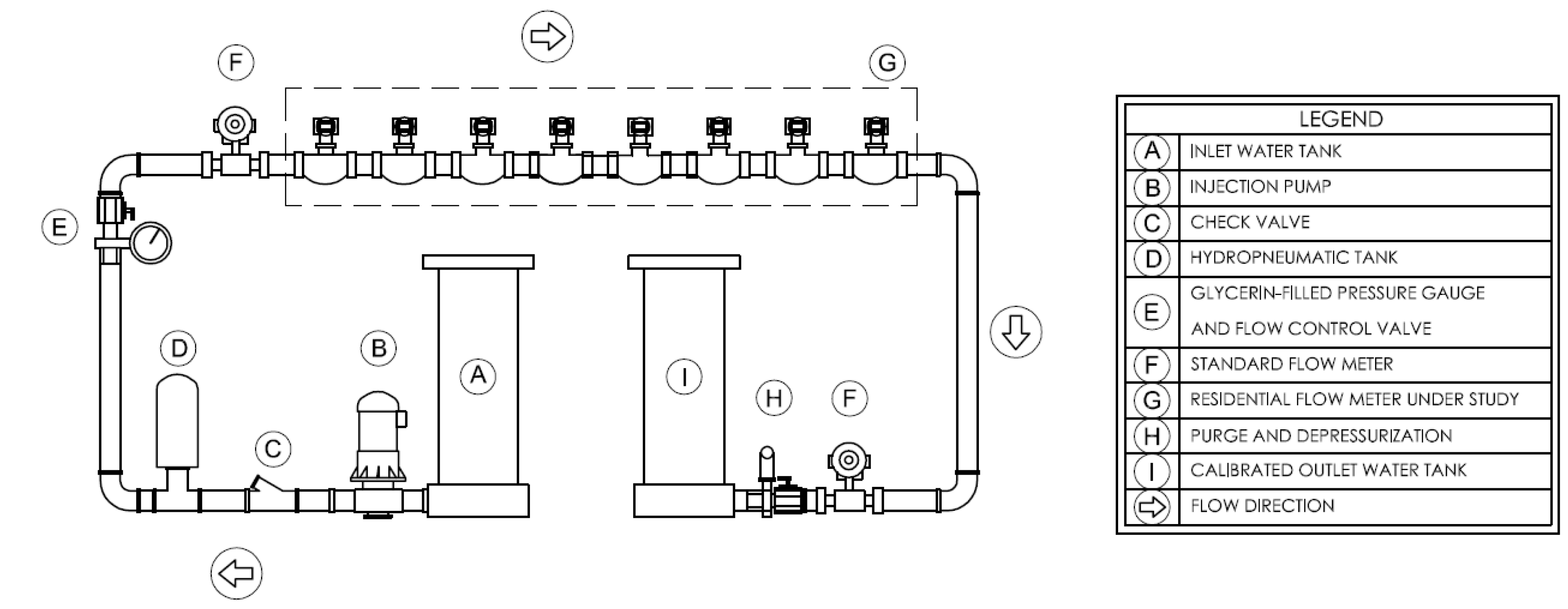
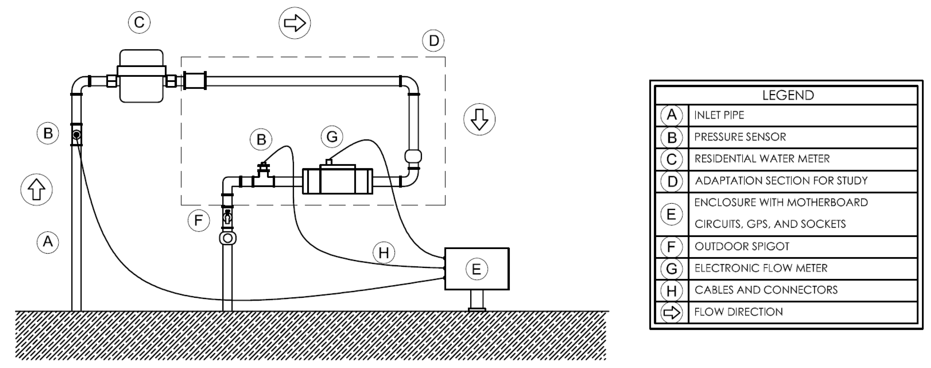
2.2.4. Hydraulic Water Meter Bench
2.2.5. Water Meters Tested
2.2.6. Limitation of the Study
3. Results
Expected and Obtained Data
4. Discussion of Results
5. Conclusions
Author Contributions
Funding
Data Availability Statement
Acknowledgments
Conflicts of Interest
References
- Alegre, H.; Baptista, J.M.; Cabrera, E.; Cubillo, F.; Duarte, P.; Hirner, W.; Merkel, W.; Parena, R. Performance Indicators for Water Supply Services, 2nd ed.; IWA Publishing: London, UK, 2013. [Google Scholar] [CrossRef]
- Ingeduld, P.; Pradhan, A.; Svitak, Z.; Terrai, A. Modelling intermittent water supply systems with EPANET. In Proceedings of the 8th Annual Water Distribution Systems Analysis Symposium, Cincinnati, OH, USA, 27–30 August 2006; pp. 1–8. [Google Scholar] [CrossRef]
- Machell, J.; Boxall, J. Field Studies and Modeling Exploring Mean and Maximum Water Age Association to Water Quality in a Drinking Water Distribution Network. J. Water Resour. Plan. Manag. 2012, 138, 624–638. [Google Scholar] [CrossRef]
- Blokker, E.M.; Furnass, W.R.; Machell, J.; Mounce, S.R.; Schaap, P.G.; Boxall, J.B. Relating Water Quality and Age in Drinking Water Distribution Systems Using Self-Organising Maps. Environments 2016, 3, 10. [Google Scholar] [CrossRef]
- Cancela, J.J.; Álvarez, C.J.; Fandiño, M. Characterization of Irrigated Holdings in the Terra Chá Region of Spain: A First Step Towards a Water Management Model. Water Resour. Manag. 2005, 19, 23–36. [Google Scholar]
- Grayman, W.; Murray, R.; Savić, D. Effects of Redesign of Water Systems for Security and Water Quality Factors. In Proceedings of the World Environmental and Water Resources Congress, Kansas City, MI, USA, 17–21 May 2009; pp. 1–11. [Google Scholar]
- Piazza, S.; Sambito, M.; Freni, G. A Novel EPANET Integration for the Diffusive–Dispersive Transport of Contaminants. Water 2022, 14, 2707. [Google Scholar] [CrossRef]
- Piazza, S.; Sambito, M.; Freni, G. Analysis of diffusion and dispersion processes in water distribution networks through the use of the Péclet number threshold. IOP Conf. Ser. Earth Environ. Sci. 2023, 1136, 012049. [Google Scholar] [CrossRef]
- Criminisi, A.; Fontanazza, C.M.; Freni, G.; Loggia, G.L. Evaluation of the apparent losses caused by water meter under-registration in intermittent water supply. Water Sci. Technol. 2009, 60, 2373–2382. [Google Scholar] [CrossRef]
- Abuiziah, I.; Oulhaj, A.; Sebari, K.; Ouazar, D. Sizing the protection devices to control water hammer damage. Int. J. Civil Strct. Constr. Architectural Eng. 2013, 7, 558–563. [Google Scholar]
- Alvisi, S.; Franchini, M. Water distribution systems: Using linearized hydraulic equations within the framework of ranking-based optimization algorithms to improve their computational efficiency. Environ. Model. Softw. 2014, 57, 33–39. [Google Scholar] [CrossRef]
- Wiek, A.; Larson, K.L. Water, people, and sustainability—A systems framework for analyzing and assessing water governance regimes. Water Resour. Manag. 2012, 26, 3153–3171. [Google Scholar] [CrossRef]
- Buchberger, S.G.; Wu, L. Model for Instantaneous Residential Water Demands. J. Hydraul. Eng. 1995, 121, 232–246. [Google Scholar] [CrossRef]
- Alcocer-Yamanaka, V.H.; Tzatchkov, V.G.; Arreguín-Cortes, F.I. Modeling of Drinking Water Distribution Networks Using Stochastic Demand. Water Resour. Manag. 2012, 26, 1779–1792. [Google Scholar] [CrossRef]
- Agnew, M.D.; Goodess, C.M.; Hemming, D.; Giannakopoulos, C.; Salem, S.B.; Bindi, M.; Bradai, M.N.; Congedi, L.; Dibari, C.; El-Askary, H.; et al. Chapter 1: Introduction. In Regional Assessment of Climate Change in the Mediterranean: Case Studies; Springer International Publishing: Dordrecht, The Netherlands, 2013; pp. 3–21. [Google Scholar]
- Gnavi, L.; Taddia, G.; Russo, S.L. Assessment and Risk Management for Integrated Water Services. In Engineering Geology for Society and Territory; Springer International Publishing: Berlin, Heidelberg, Germany, 2015; Volume 6, pp. 653–656. [Google Scholar]
- Creaco, E.; Farmani, R.; Vamvakeridou-Lyroudia, L.; Buchberger, S.G.; Kapelan, Z.; Savić, D.A. Correlation or not Correlation? This is the Question in Modelling Residential Water Demand Pulses. Procedia Eng. 2015, 119, 1455–1462. [Google Scholar] [CrossRef]
- Chang, N.-B.; Pongsanone, N.P.; Ernest, A. A rule-based decision support system for sensor deployment in small drinking water networks. J. Clean. Prod. 2013, 60, 152–162. [Google Scholar] [CrossRef]
- Creaco, E.; Alvisi, S.; Farmani, R.; Vamvakeridou-Lyroudia, L.; Franchini, M.; Kapelan, Z.; Savic, D.A. Preserving Duration-intensity Correlation on Synthetically Generated Water Demand Pulses. Procedia Eng. 2015, 119, 1463–1472. [Google Scholar] [CrossRef]
- Cominola, A.; Giuliani, M.; Piga, D.; Castelletti, A.; Rizzoli, A.E. Benefits and challenges of using smart meters for advancing residential water demand modeling and management: A review. Environ. Model. Softw. 2015, 72, 198–214. [Google Scholar] [CrossRef]
- Jiménez-Buendía, M.; Ruiz-Peñalver, L.; Vera-Repullo, J.A.; Intrigliolo-Molina, D.S.; Molina-Martínez, J.M. Development and assessment of a network of water meters and rain gauges for determining the water balance. New SCADA monitoring software. Agric. Water Manag. 2015, 151, 93–102. [Google Scholar] [CrossRef]
- Pedro-Monzonís, M.; Solera, A.; Ferrer, J.; Estrela, T.; Paredes-Arquiola, J. A review of water scarcity and drought indexes in water resources planning and management. J. Hydrol. 2015, 527, 482–493. [Google Scholar] [CrossRef]
- Elsheikh, M.A.; Saleh, H.I.; Rashwan, I.M.; Et-Samadoni, M.M. Hydraulic modelling of water supply distribution for improving its quantity and quality. Sustain. Environ. Res. 2013, 23, 403–411. [Google Scholar]
- De Marchis, M.; Milici, B.; Freni, G. Pressure-discharge law of local tanks connected to a water distribution network: Experimental and mathematical results. Water 2015, 7, 4701–4723. [Google Scholar] [CrossRef]
- Salman, D.A.; Amer, S.A.; Ward, F.A. Water Appropriation Systems for Adapting to Water Shortages in Iraq. JAWRA J. Am. Water Resour. Assoc. 2014, 50, 1208–1225. [Google Scholar] [CrossRef]
- Arregui, F.; Cabrera, E.; Cobacho, R. Integrated Water Meter Management; Water Intelligence Online; IWA Publishing: London, UK, 2006. [Google Scholar]
- Buchberger, S.G.; Carter, J.T.; Lee, Y.; Schade, T.G. Random Demands, Travel Times and Water Quality in Deadends; Prepared for American Water Works Association Research Foundation; Report No. 294; AWWA Research Foundation and National Science Foundation: Denver, CO, USA, 2003. [Google Scholar]
- Saurí, D. Water conservation: Theory and evidence in urban areas of the developed world. Annu. Rev. Environ. Resour. 2013, 38, 227–248. [Google Scholar] [CrossRef]
- Marlow, D.R.; Moglia, M.; Cook, S.; Beale, D.J. Towards sustainable urban water management: A critical reassessment. Water Res. 2013, 47, 7150–7161. [Google Scholar] [CrossRef] [PubMed]
- Klepka, A.; Broda, D.; Michalik, J.; Kubat, M.; Malka, P.; Staszewski, W.J.; Stepinski, T. Leakage detection in pipelines-the concept of smart water supply system. In Proceedings of the 7th ECCOMAS Thematic Conference on Smart Structures and Materials, Ponta Delgada, Azores, Portugal, 3–6 June 2015; pp. 3–6. [Google Scholar]
- Martinez, F.; Conejos, P.; Vercher, J. Developing an integrated model for water distribution systems considering both distributed leakage and pressure-dependent demands. In Proceedings of the 1999 ASCE Water Resources Conference, Tempe, AZ, USA, 6–9 June 1999. [Google Scholar]
- Davis, S.E. Residential water meter replacement economics. In Proceedings of the IWA Leakage 2005 Conference, Halifax, NS, Canada, 12–14 September 2005; pp. 1–10. [Google Scholar]
- Creaco, E.; Kossieris, P.; Vamvakeridou-Lyroudia, L.; Makropoulos, C.; Kapelan, Z.; Savic, D. Parameterizing residential water demand pulse models through smart meter readings. Environ. Model. Softw. 2016, 80, 33–40. [Google Scholar] [CrossRef]
- Creaco, E.; Alvisi, S.; Farmani, R.; Vamvakeridou-Lyroudia, L.; Franchini, M.; Kapelan, Z.; Savic, D. Methods for Preserving Duration–Intensity Correlation on Synthetically Generated Water-Demand Pulses. J. Water Resour. Plan. Manag. 2015, 142, 06015002. [Google Scholar] [CrossRef]
- Spiliotis, M.; Tsakiris, G. Water distribution network analysis under fuzzy demands. Civ. Eng. Environ. Syst. 2012, 29, 107–122. [Google Scholar] [CrossRef]


| Comparison of Alternative Models | ||
|---|---|---|
| Model | Correlation | Square Root |
| Multiplicative | 0.9418 | 88.70% |
| Double square root | 0.9343 | 87.29% |
| Square root of X | 0.9115 | 83.09% |
| Square root-Y Log-X | 0.8958 | 80.25% |
| Logarithmic-Y square root-X | 0.8876 | 78.79% |
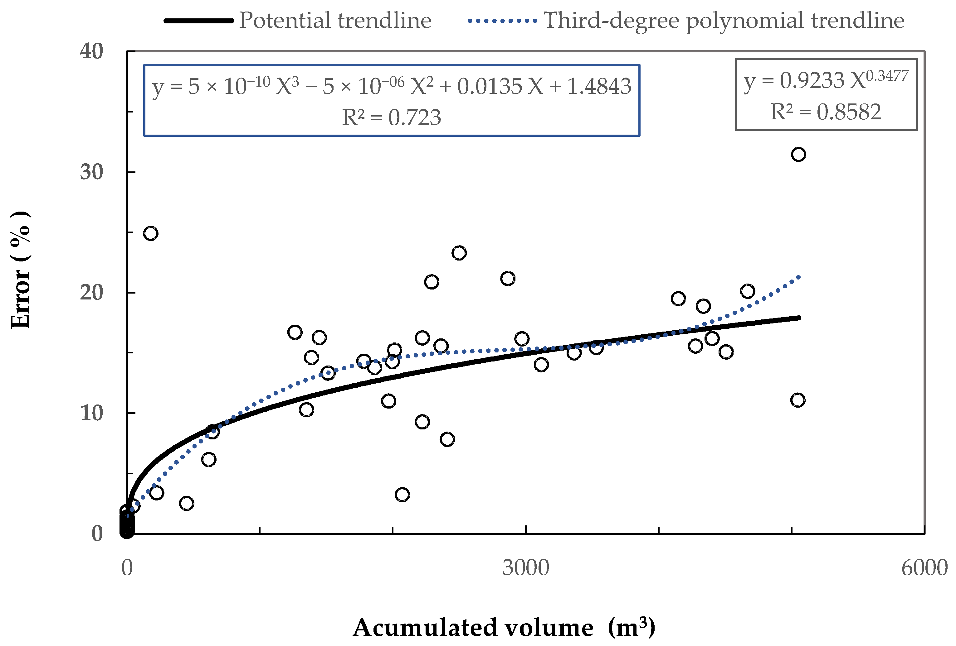
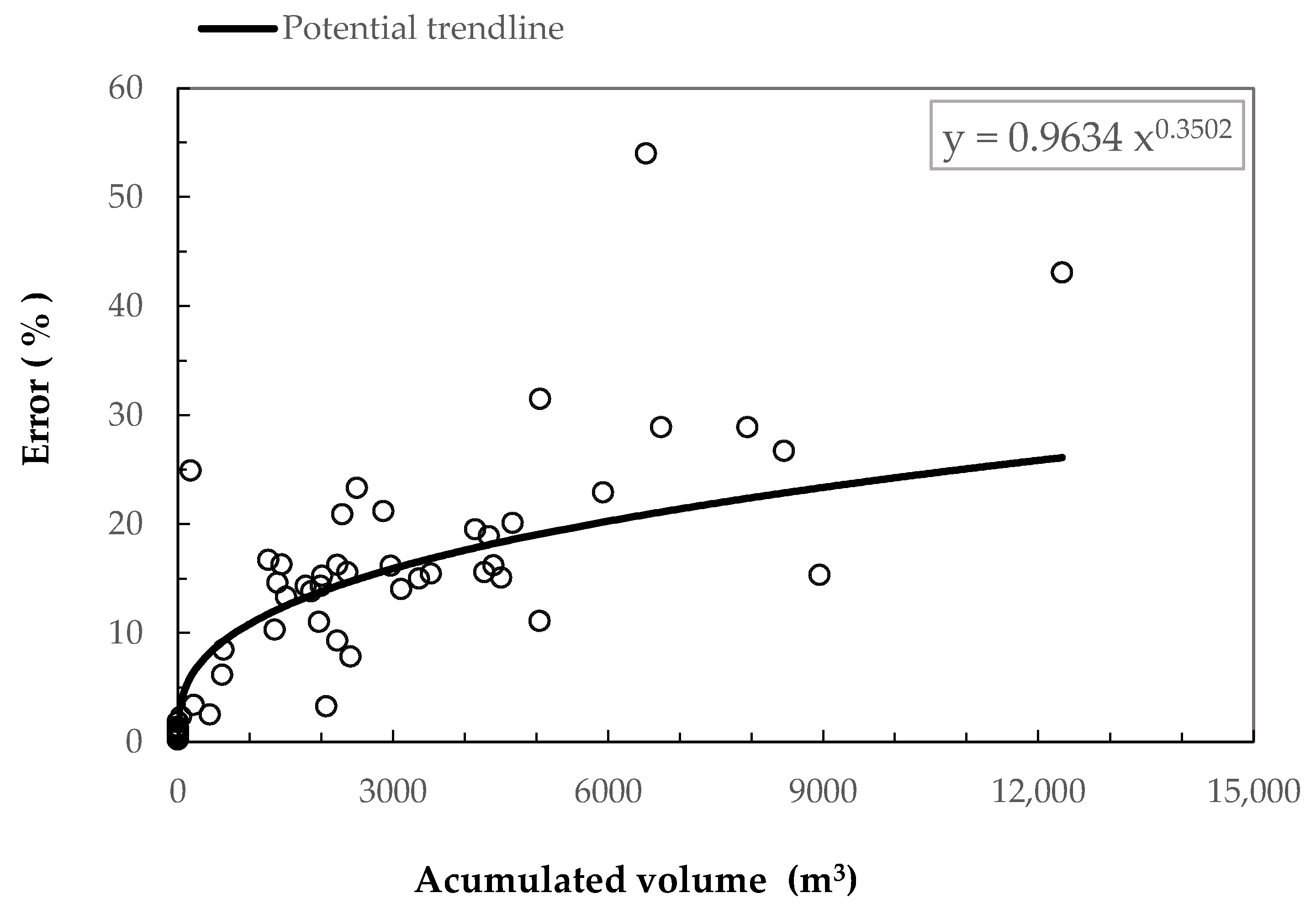
| Volume (m3) | Error (%) |
|---|---|
| 100 | 4.82 |
| 500 | 8.48 |
| 1000 | 10.81 |
| 3000 | 15.88 |
| 5000 | 18.99 |
| 8000 | 22.38 |
| 10,000 | 24.20 |
Disclaimer/Publisher’s Note: The statements, opinions and data contained in all publications are solely those of the individual author(s) and contributor(s) and not of MDPI and/or the editor(s). MDPI and/or the editor(s) disclaim responsibility for any injury to people or property resulting from any ideas, methods, instructions or products referred to in the content. |
© 2023 by the authors. Licensee MDPI, Basel, Switzerland. This article is an open access article distributed under the terms and conditions of the Creative Commons Attribution (CC BY) license (https://creativecommons.org/licenses/by/4.0/).
Share and Cite
Benavides-Muñoz, H.M.; Medina-Armijos, B.; González-González, R.; Martínez-Solano, F.J.; Lapo-Pauta, M. Temporal Fluctuations in Household Water Consumption and Operating Pressure Related to the Error of Their Water Meters. Water 2023, 15, 1895. https://doi.org/10.3390/w15101895
Benavides-Muñoz HM, Medina-Armijos B, González-González R, Martínez-Solano FJ, Lapo-Pauta M. Temporal Fluctuations in Household Water Consumption and Operating Pressure Related to the Error of Their Water Meters. Water. 2023; 15(10):1895. https://doi.org/10.3390/w15101895
Chicago/Turabian StyleBenavides-Muñoz, Holger Manuel, Byron Medina-Armijos, Rutbel González-González, Francisco Javier Martínez-Solano, and Mireya Lapo-Pauta. 2023. "Temporal Fluctuations in Household Water Consumption and Operating Pressure Related to the Error of Their Water Meters" Water 15, no. 10: 1895. https://doi.org/10.3390/w15101895