Dry Weight Prediction of Wedelia trilobata and Wedelia chinensis by Using Artificial Neural Network and MultipleLinear Regression Models

1
State Key Laboratory of Desert and Oasis Ecology, Xinjinag Institute of Ecology and Geography, Chinese Academy of Sciences, Urmuqi 830011, China
2
School of the Environment and Safety Engineering, Jiangsu University, Zhenjiang 212013, China
*
Authors to whom correspondence should be addressed.
Water 2023, 15(10), 1896; https://doi.org/10.3390/w15101896
Submission received: 6 February 2023
/
Revised: 12 May 2023
/
Accepted: 13 May 2023
/
Published: 17 May 2023
(This article belongs to the Section Ecohydrology)
Abstract
:In China, Wedelia trilobata (WT) is among the top most invasive plant species. The prediction of its growth, using different efficient methods under different environmental conditions, is the optimal objective of ecological research. For this purpose, Wedelia trilobata and its native plant species Wedelia chinensis (WC) were grown in mixed cultures under different levels of submergence and eutrophication. The multiple linear regression (MLR) and artificial neural network (ANN) models were constructed, with different morphological traits as the input in order to predict dry weight as the output for both plant species. Correlation and stepwise regression analysis (SWR) were used to find the best input variables for the ANN and MLR models. Plant height, number of nodes, chlorophyll content, leaf nitrogen, number of leaves, photosynthesis, and stomatal conductance were the input variables for WC. The same variables were used for WT, with the addition of root length. A network with the Levenberg–Marquart learning algorithm, back propagation training algorithm, Sigmoid Axon transfer function, and one hidden layer, with four and six neurons for WC and WT, respectively, was created. The best ANN model for WC (7-4-1) has a coefficient of determination (R2) of 0.98, root mean square error (RMSE) of 0.003, and mean absolute error (MAE) of 0.001. On the other hand, the ANN model for WT (8-6-1) has R2 0.98, RMSE 0.018, and MAE 0.004. According to errors and coefficient of determination values, the ANN model was more accurate than the MLR one. According to the sensitivity analysis, plant height and number of nodes are the most important variables that support WT and WC growth under submergence and eutrophication conditions. This study provides us with a new method to control invasive plant species’ spread in different habitats.
1. Introduction
Invasive plant species present a major threat to native diversity. After all, they can grow in every habitat [1]. Globalization and human exchange over the last twenty years facilitated the introduction of several plant species to novel terrestrial regions [2]. After introduction into new habitats, some plant species become invasive plants in these novel environments, and destructively affect the ecosystem, economy, and culture [3]. Invasive plant species can capture resources from above and below ground [4]. These abilities enable them to overcome the growth of their native competitor under mixed culture [5]. Understanding the mechanisms by which invasive plant species sustain their growth under different environmental conditions is crucial for their management [6].
The role of functional traits is very important for the successful invasion of invasive plant species under different habitat conditions [7]. Functional traits also assist invasive plant species in boosting their growth under competition, and reduce the growth of their native competitor [8]. Functional trait responses under different habitat conditions, such as nutrient availability, water fluctuation, and temperature variation, greatly impact invasive plant species’ effective invasion and the growth of native plants [9]. Different functional traits play a different role in the effective invasion of these invasive plant species; for example, root and shoot functional traits are indicators of growth development [10]. Additionally, photosynthesis, transpiration, and evaporation are the main indicators of leaf growth development [11]. Therefore, understanding the responses of functional traits under different environmental conditions is very fruitful for managing invasive plant species.
Considering globalization, many environmental factors, i.e., water, nutrients, CO2, light, and temperature, affect the growth of native plant species, but assist invasive plant species in sustaining their development because they prefer to grow in disturbed habitats [6]. In wetland or riparian zones, the main issues are submergence and eutrophication. The former, called submergence, is a type of flooding during which the shoot of a plant is under water [12]. Expulsion of water from riversides, dams, and canals will create submergence close to these areas, and vegetation will face submergence. Submergence imposes considerable stress by decreasing energy and carbohydrate values [13]. Functional traits, such as shoot elongation and leaves, assist both invasive and native plant species in sustaining their growth under submergence, by enabling exposure to sunlight for photosynthesis [5,14]. Eutrophication is another environmental factor that negatively affects the aquatic ecosystem [15]. Eutrophication decreases the growth of native plant species. It boosts the growth of invasive plant species because invasive plant species prefer to grow in an environment with rich resources [16]. Eutrophication helps to overcome the stress of submergence by enhancing the shoot of invasive species because these plants can obtain more CO2, light for photosynthesis, and oxygen for transpiration [14]. Meanwhile, invasive plant species enhance their root length in order to capture resources below ground, and overcome the growth of their native competitor by enhancing their root length [17]. Therefore, for managing invasive plant species under submergence and eutrophication habitats, the traits of different growth parameters assist us in understanding their invasion.
Growth parameters play the main role in successfully invading invasive plant species under different habitats, especially under competition. In the agriculture sector, many growth prediction models have been developed with the help of varying growth parameters, under additional irrigation and planting methods [18,19,20]. Most modeling for the prediction of growth was done with the help of different statistical techniques such as correlation, path analysis, multiple linear regression (MLR), stepwise regression (SWR), factor analysis, and principal component analysis (PCA) [21,22,23]. All of these methods presume to follow the linear relationship of input and output. These methods could not explain the complex relationship among the input variables and the output [24]. These complex relationships required non-linear methods, such as Bayesian classification (BC), artificial neural network (ANN) models, genetic expression programming (GEP), and adaptive neuro-fuzzy inference systems (ANFIS) in order to overcome the drawback of these linear models and provide more accurate results [25,26,27]. The ANN model is most commonly used for modeling crop yield in agriculture [28]. It is a mathematical tool that attempts to represent low-level intelligence in normal creatures. The construction of ANN models is fairly basic, and it may create a non-linear relationship between the input and output variables [29]. The neuron types, training technique, transfer function, and hidden layer of ANN models are used to classify them [30]. Multi-layer perceptron (MLP) networks are commonly used for ANN modeling in the agriculture sector [23,31].
These non-linear complex models were created in order to forecast the growth prediction of different crops by using their growth parameters as input variables [21,22,28]. In the ecological sector, there is a lack of research with the help of these non-linear complex models being used to forecast the growth of invasive plants. Furthermore, there is no study using the ANN model to predict the growth of invasive plants under different environmental conditions, in China or all over the world, even though invasive plant species are major threat to native biodiversity. The ANN model must be constructed in order to predict invasive plant species responses under different environmental conditions.
Furthermore, the hypothesis of this study that these predicting models describe to us would help to control the growth of these invasive species under native biodiversity. As a result, this work aimed to develop ANN and MLR models that could predict which growth parameters help Wedelia trilobata and its native species, Wedelia chinensis, to survive under submergence and eutrophication. Furthermore, predicting which growth parameters of Wedelia trilobata would reveal the important factors that allow it to overcome the growth of its native competitor under competition within submergence and eutrophication. These prediction models could be very helpful for managing invasive plant species under submergence and eutrophication habitats.
2. Materials and Methods
Wedelia trilobata (WT) is among the top most invasive plants in China [6]; WT and Wedelia chinensis (WC) both come from the Asteraceae family [3]. It was mostly found worldwide in arid, semiarid, and humid regions [9]. It is familiar as a groundcover plant species in China, but over time, it moved speedily from gardens to the roadside and finally into agricultural fields. It is also found in the wetland areas near the riverside [1]. This likely indicates that WT can sustain its growth under submergence and eutrophication.
2.1. Study Site and Material Preparation
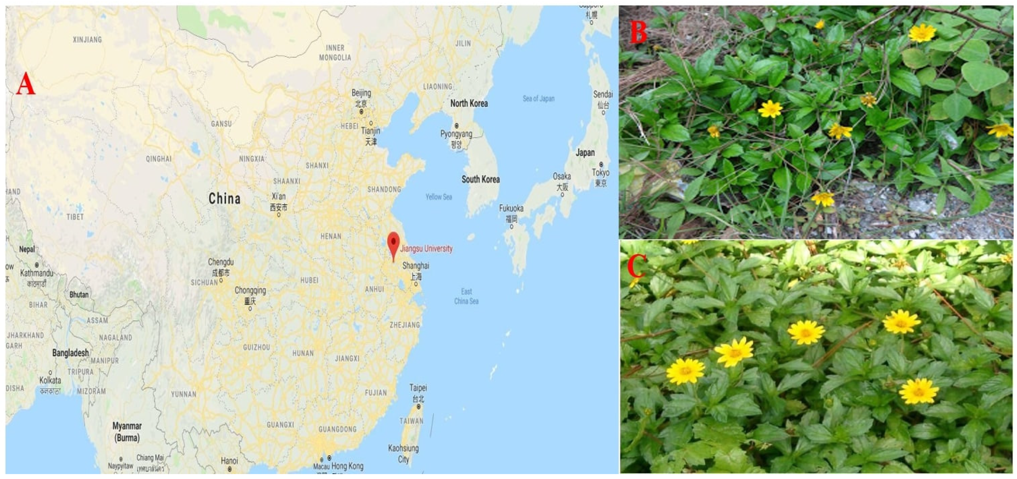
Plant material (Ramets) of WT and WC were collected around the Yangtze River bank (29.7204° N, 112.6501° E), in Yangzhou, Jiangsu, China. Ramets of both plant species were harvested after obtaining necessary approval, and all processes were conducted in compliance with applicable standards and laws. It is considered a cultivation study because ramets of both plant species have been used. This experiment was conducted in the greenhouse of Jiangsu University (32.1993° N, 119.5143° E), Zhenjiang, Jiangsu China, from the start of September to 20 November 2019, as presented in Figure 1. In the seedling tray, ramets of WT and WC were prepared with sandy soil and peat moss (1:1) as growth media for the experimental investigation. These seedling trays were kept in a greenhouse with a temperature of 30 ± 5 °C and a relative humidity of 60%. Seedlings were watered every day, and Hoagland solution was applied once a week.
When the prepared seedlings had two completely grown leaves, then these seedlings were shifted into plastic pots (12.7 cm height and 17.78 cm diameter) filled with sandy soil as a growth medium. Pots of these seedlings were located in a bin (80 × 40 × 20 cm) for mesocosm investigation within the greenhouse. Both species were grown together in mixed culture, with 15 replicates of every treatment. For one week, normal water was provided to the seedlings to allow them to sustain in their new habitat condition. After 7 days, these transplanted seedlings were divided into 2 submergence and 3 eutrophication levels in order to simulate the naturally existing submergence and eutrophication under the wetland environment. There were two submergence stages (S1 = 7 cm and S2 = 14 cm) and three nutrient groups—N1 containing nitrogen (0.45 mg/L) and phosphorus (0.097 mg/L); N2 containing nitrogen (4.5 mg/L) and phosphorus (0.97 mg/L); and N3 containing nitrogen (45 mg/L) and phosphorus (9.7 mg/L),—using KNO3, NH4Cl, and KH2PO4 to prepare each of these treatments, respectively [5]. There were 90 pots in total. Every day, tap water was added to each treatment bin to maintain the submergence level, and the nutrient solution was renewed one time after seven days. Plants were harvested after 30 days.
2.2. Morphological Trait Measurement
Plant height and root length of the plants from each treatment were measured with a ruler at the time of harvesting. ImageJ software was used to measure leaf area; the number of leaves and nodes were counted at the time of harvesting for the plants from every treatment. The dry weight (DW) of each plant per treatment was measured after drying at ≤80 °C for 48 h. The specific leaf area was calculated using the formula of leaf area to dry mass.
A portable LI-6400XT photosynthesis measurement instrument was used to measure the photosynthesis, transpiration, and stomatal conductance of the plants from each treatment. A fully expanded leaf was selected for measurement. Measurement was taken from 10.00 to 11.00 am under full sunshine. Using LI-6400XT, the following settings were noted during the measurement of data: atmospheric pressure 98.9 kpa, air molar flow 402.5 mmol m−2s−1, photosynthetically active radiation up to 1000 μmol m−2 s−1, CO2 concentration 402 μmol mol−1, vapor pressure 7.0 to 8.8 mbar, and ambient temperature 30.2 to 34.8 °C.
The water potential of each plant that underwent treatment was calculated using Psypro, Wescor, USA before harvesting of plants. Details of the growth parameters, along with their units and abbreviations, are presented in Abbreviations Part.
2.3. Processing of Data and Statistical Analysis
2.3.1. Criteria for Input Variables
The dataset’s normality was checked with the Anderson–Darling test using SPSS 22 statistical software. Pearson correlation coefficients and stepwise regression (SWR) were used to assess the association between the morphological features and DW using SPSS 22 statistical software. Statistica software was used to run the ANN models, which used DW as the dependent and other features as independent parameters [22]. Nightly samples were used to train, test and validate the ANN model. The descriptive statistics of the trait variables of both plant species are presented in Table 1 and Table 2.
2.3.2. Artificial Neural Network (ANN)
The dry weights (DWs) of both plant species, WT and WC, were used as output variables. In contrast, the remaining parameters were used as input variables. ANN training and testing were done based on the morphological traits of the invasive plant species under the submergence and eutrophication experiments. All datasets were divided into training, testing, and validation by a 70:15:15% ratio. This selection was done according to the previous literature [24].
All data have been normalized and placed within the data ranges, where the Tanh [–1, 1] and Sigmoid [0, 1] are activation functions [32]. For normalization, Equation (1) was utilized.
where Xnorm is the normalized value of an independent or dependent variable. Xmin and Xmax are the variable’s minimum and maximum values, and Xi’s are the original data.
The optimal neural network structure contains three primary layers: input, hidden, and output. The output of the network is presumed via Equation (2).
Yf represents the model output (DW), n and m represent the hidden layers and input nodes, and the transfer function is donated by f. Cij i = 1, 2, …, m; j = 0, 1, …, n is the weight from the input through the hidden node, and dj j = 0, 1,…, n are the weight vectors extending from the hidden layers to the output nodes. The weight of leading arcs from bias terms, denoted by a0 and b0j, are always equal to 1. Based on earlier research [21,22,32], the current study used a feed-forward multi-layer perceptron (MLP) topology with three layers, and the back propagation (BP) training technique, along with the Levenberg–Marquardt, Momentum, and Conjugate Gradient learning algorithms. Trial-and-error testing was used to identify hidden layers (1–3) and neurons [25]. Sigmoid Axon, Tangent Hyperbolic Axon, Linear Sigmoid Axon, and Linear Tangent Hyperbolic Axon activation functions were used to determine the best equation with high accuracy within the hidden and output layers [33,34].
2.3.3. Multiple Linear Regression (MLR)
Stepwise regression analysis (SWR) was conducted in order to determine the relative contributions of independent variables and to create a prediction model for the DW of WT and WC [35]. Equation (3) was used to generate the SWR model using the same data as the ANN model. Independence of error was determined using the Durbin–Watson test. The tolerance value and variance inflation factor (VIF) were also tested in order to check the occurrence of multicollinearity for predictor variables. Higher collinearity described a smaller tolerance value (<0.1) or a high VIF (>10) value.
where a0 + an is the regression coefficient, X1 − Xn are independent variables, and € is the error of the nth observation.
2.3.4. Performance and Sensitivity Analysis
As demonstrated in Equations (4)–(6) [36], the accuracy of the ANN and MLR models was evaluated using the root mean square error (RMSE), coefficient of determination (R2), and mean absolute error (MAE).
where n represents the number of data, Yi denotes the actual value, and Yj denotes the predicted value. Yio and Yjo are the mean values of observed and predicted values, respectively. A model with lower values of RMSE and MAE and a higher value of R2 is considered the best prediction model.
Sensitivity analysis was performed by choosing the most appropriate input parameters that control the dry weight of WT and WC within submergence and eutrophication, after determining the best ANN model. The sensitivity analysis was performed by running a dataset without any input variables, and the values of R2, RMSE, and MAE determined the accuracy of the model [37].
3. Results and Discussion
3.1. Selection of Input Variables
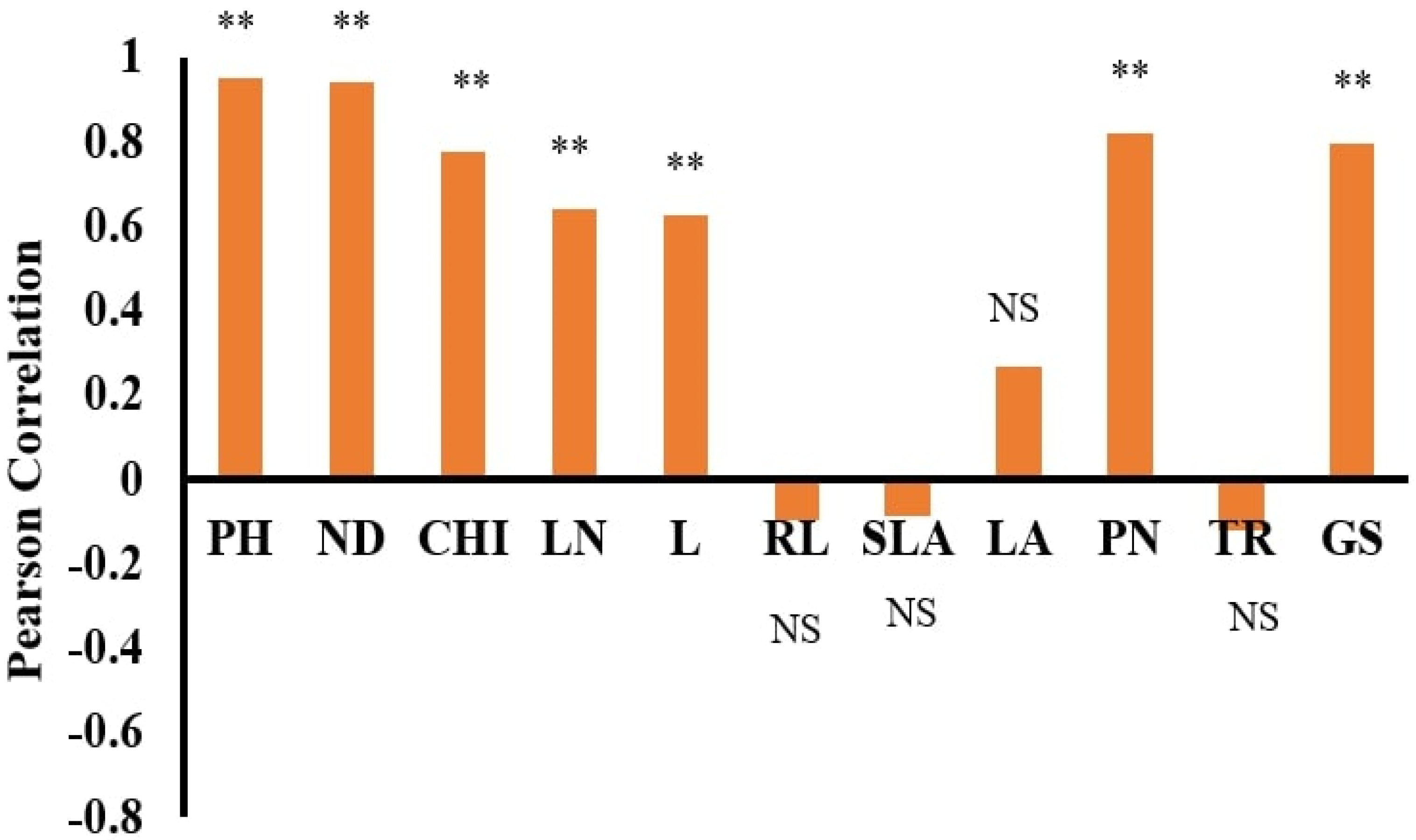
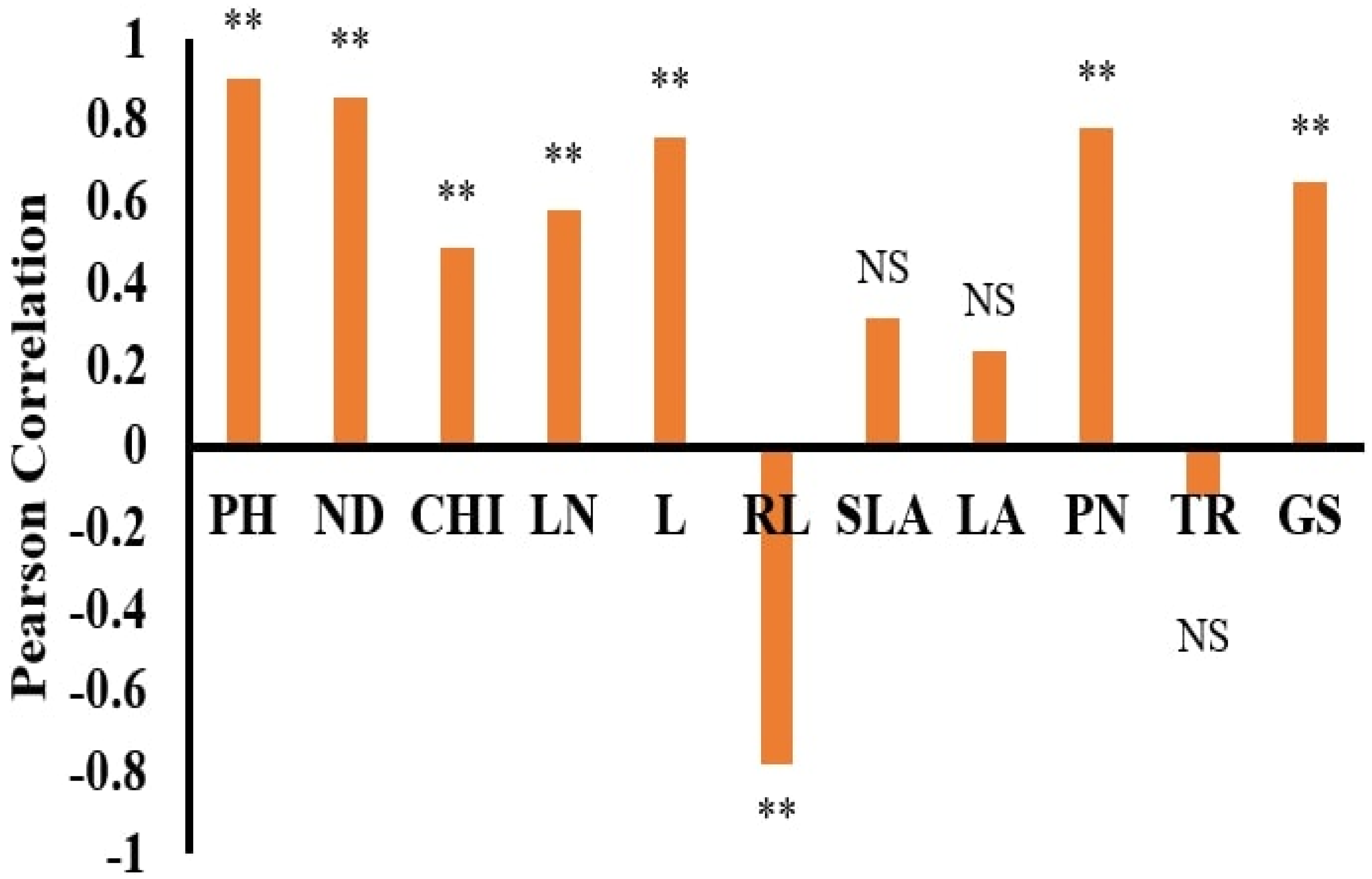
The selection of input parameters is crucial for developing a model. These input factors have a major impact on the weighted coefficient and the model’s final design [23]. Therefore, this phase is critical for determining the optimum function for statistical models such as ANN and MLR. A Pearson correlation coefficient was used to assess the association between the DWs of WT and WC. Figure 2 and Figure 3 demonstrate WC and WT with various features used as input variables. WC demonstrates a strong positive correlation with PH (R2 = 0.951), followed by ND (R2 = 0.943), CHI (R2 = 0.777), LN (R2 = 0.643), L (R2 = 0.626), PN (R2 = 0.819), and GS (R2 = 0.795). WT also demonstrates a positive correlation with PH (R2 = 0.906), followed by ND (R2 = 0.859), CHI (R2 = 0.488), LN (R2 = 0.550), L (R2 = 0.761), PN (R2 = 0.781), and GS (R2 = 0.448). At the same time, WT negatively correlates with RL (R2= −0.780). A negative correlation of WT and RL, under competition due to phenotyping plasticity, help WT to capture resources below ground and destroy the growth of WC [5]. The negative correlation of RL also makes WT a stronger competitor in capturing resources below ground [12]. Under submergence and eutrophication, the plant height and number of leaves facilitate the plant’s exposure to sunlight in order to alleviate the negative effects of submergence and eutrophication [14] and continue their photosynthetic process for growth development [9]. Therefore, according to previous studies [9,14,38], and this study’s correlation results, it can be postulated that PH, ND, CHI, LN, L, RL, PN GS are the most important trait parameters to determining the DW of WT and WC, as presented in Figure 2 and Figure 3.
In addition to the correlation coefficient, stepwise regression analysis (SWR) was performed to counter-check the relationship between the trait variables and DW. Correlation within different parameters can be disturbed by the positive and negative incidental effects of other variables; this problem disturbs the efficiency of selecting input variables [39,40]. The authors of Refs. [21,22] also described that SWR is the best method for selecting input variables and increasing the model’s efficiency. Therefore, SWR was performed in order to determine the best input trait variables. According to the SWR, PH, ND, CHI, LN, L, PN, and GS were considered to be the most appropriate input variables for the ANN and MLR models for WC under submergence and eutrophication in Table 3.
Meanwhile, similar input variables were found for WT under SWR only with the addition of RL, as presented in Table 4. SWR reduced the number of input variables because it only selected the more efficient model development variable [41,42]. While in our study, results of correlation and SWR have the same because all these growth trait variables greatly influence the DW of WT and WC within submergence and eutrophication [5].
3.2. Prediction of Dry Weight of Wedelia trilobata and Wedelia chinensis Using ANN
After selecting the appropriate input variables for model development, selecting the transfer function, hidden layers, and their neurons are important for optimal model development. These can be determined by trial and error [43,44]. For this purpose, four different transfer functions—Tangent Hyperbolic Axon, Sigmoid Axon, Linear Tangent Hyperbolic Axon, and Linear Sigmoid Axon—were used in order to determine the best transfer function, as presented in Table 5. Learning algorithms and different transfer functions were used to assess the efficiency of the ANN model [45]. The lowest RMSE and MAE, and higher R2, were determined by using the Sigmoid Axon as a transfer function for both plant species in the testing, training, and validation phase, as presented in Table 6. These findings could be related to the transfer function. It is possible that the input variables and output in this study revealed a complex non-linear relationship; meanwhile, it can be obtained that the Sigmoid Axon function can cover complex non-linear variations related to other transfer functions [24]. Many crop growth prediction models utilized the Sigmoid Axon transfer function [21,22,25,46].
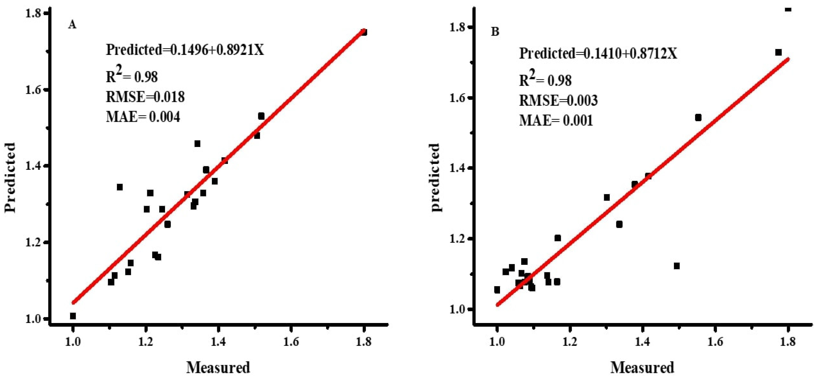
After selecting the optimum transfer function, the various numbers of hidden layers were examined in order to determine the best number of hidden layers for DW prediction in the ANN model [32]. Based on the values of RMSE, MAE, and R2 under different hidden layers, the optimum results in testing (RMSE = 0.003, MAE = 0.001, and R2 = 0.98), training (RMSE = 0.047, MAE = 0.027, and R2 = 0.98), and validation (RMSE = 0.28, MAE = 0.16, and R2 = 0.99), for WC were determined, with one hidden layer, along with four neurons. Similarly, for WT, testing (RMSE = 0.018, MAE = 0.004, and R2 = 0.98), training (RMSE = 0.008, MAE = 0.004, and R2 = 0.99), and validation (RMSE = 0.23, MAE = 0.16, and R2 = 0.99) were determined, also with one hidden layer, along with six neurons, as presented in Table 6. The transfer function between hidden layers and nodes, exhibiting the complexity of the ANN, is one of the most important elements influencing the accuracy and performance of the ANN [32]. Increasing the number of hidden layers and neurons did not affect performance and accuracy of the model discussed in this work [26]. The total input, the output variables, the algorithm used for training, the complexity of the ANN structure, and the number of samples used for the training network are the elements that can disturb hidden layers and units in the ANN [32,47,48,49].
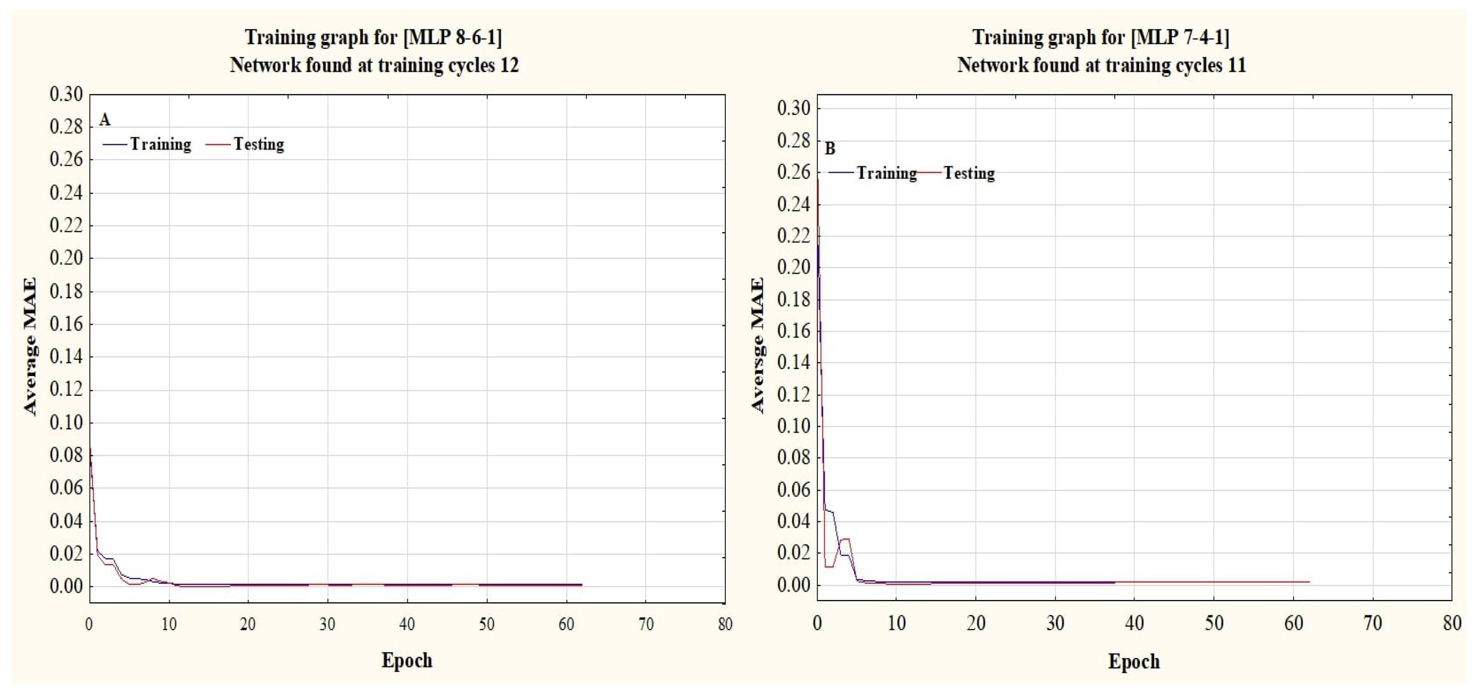
Back propagation training algorithms, along with Levenberg–Marquardt learning algorithms containing the Sigmoid Axon transfer function, with seven input variables in the input layer for WC and eight input variables for WT, one hidden layer having four neurons within each layer for WC, and one hidden layer having six neurons within each layer for WT, along with one output for both plant species, were used to build ANN models for both plant species. As depicted in Table 6, the optimum topology of the ANN model used to determine the DW of both plant species is 7-4-1 for WC and 7-6-1 for WT. The selection criteria of the best predicted ANN model should hold the minimum hidden layers, fewer neurons, and higher performance values [50,51], which were considered in these predicted models. Many epochs can reduce the ANN performance and increase the chances of memorization and overtraining [32]. A pretest, using one hidden layer and many epochs (10–500), was conducted in order to reduce overtraining and memorization. Figure 4 depicts the convergence point within training and testing where the conclusion of training time will avoid overtraining.
Measured and predicted DW values for both plant species are presented in scatter plots, with the help of the training datasets, in Figure 5. Both predicted and estimated values exhibit the same distribution in the scatter plots, indicating non-significant results for both plant species.
3.3. Multiple Linear Regression (MLR)
MLR models were used to build models when there were linear relationships within input and output variables [52]. SWR was conducted using different input variables (PH, ND, L, LN, CHI, PN, GS, and RL) for WT and WC in order to determine the best MLR model for determining the DW of both plant species. It used the same input and output dataset to build a regression model used for the ANN model. Independence error is the main hypothesis in regression analysis. Independence error was determined according to the Durbin–Watson test, and the 1.60 value of the Durbin–Watson test indicated the independent errors in the model [53]. Non-multicollinearity, in addition to independent error, is the vital hypothesis for MLR because collinearity might result in the selection of the most significant predictor being inaccurate [54]. Tolerance and VIF values were used to check the multicollinearity hypotheses for each independent variable. The smallest tolerance values (<0.1) and higher values of VIF (>5) described high collinearity, which was found in this study, as presented in Table 3 and Table 4. MLR model equations were determined with the help of SWR analysis to predict the DW for WT and WC, as presented in Equations (7) and (8).
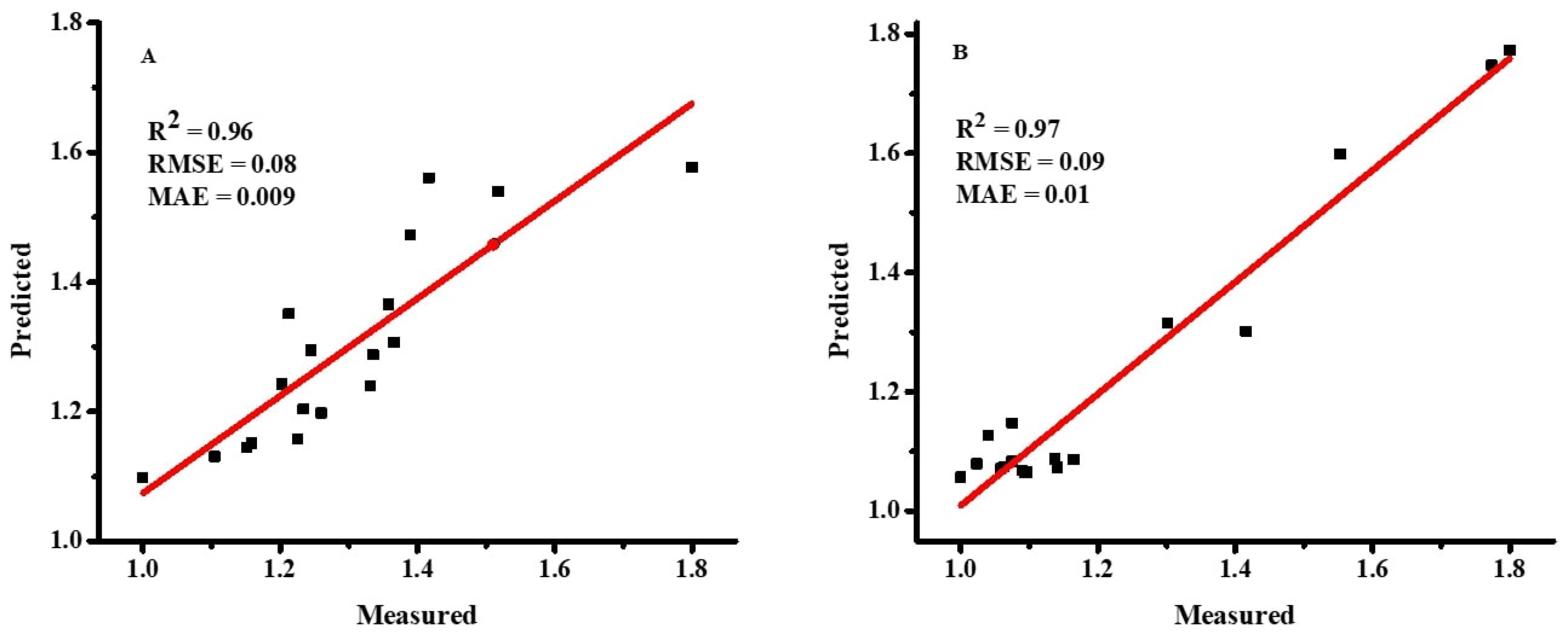
Equations (7) and (8) are the MLR equations for WT and WC, which describe the effects of the input variables on the output, and their importance. Furthermore, it also indicates how the DWs for both plant species were changed by changing the input variable datasets. The SWR analysis results determined that GS has the lowest R2 value for both WC and WT because it demonstrated less impact for DW production in both plant species [19]. On the other hand, PH has the highest R2 value for both WC and WT because it helps expose the plants to sunlight so that they can run their photosynthetic process in order to overcome the effects of submergence and eutrophication [5]. Many researchers used SWR to understand the role of the independent variables on the dependent variable for the development of regression models, i.e., in sesame (Sesamum indicum L.) and Ajowan (Trachyspermum ammi L.) [21,55]. Graphs between the predicted and measured DW values for WT and WC were created with the help of the MLR model in Figure 6. The predicted MLR model for WT has R2 = 0.96, RMSE = 0.08, and MAE = 0.009, while the Predicted MLR model for WC has R2 = 0.97, RMSE = 0.09, and MAE = 0.01, as presented in Figure 6. These errors and coefficient of determination values indicate that MLR models have low performance compared to the ANN model.
3.4. Comparsion of MLR and ANN Models
Based on the error values and coefficients of determination (R2, RMSE, and MAE), the MLR and ANN models were compared. These are the best criteria to determine the performance of differently trained models [46]. According to the results presented in the scatter plots in Figure 5 and Figure 6, the lower values of RMSE and MAE and higher values of R2 in the ANN model described that the predicted values of the ANN model are very similar to the measured values, compared to the MLR model. In short, the ANN model is more accurate in describing both plant species’ dry weights, by using different growth trait variables when compared to the MLR model because the MLR model could not describe non-linear relationships more accurately [24,25,26]. Many other researchers have agreed that the ANN model is a better method, compared to the MLR model, for the growth prediction of different crops [21,22,25,46,56].
3.5. Sensitivity Analysis
Sensitivity analysis tests were performed within the ANN and MLR models in order to understand the roles of the input variables that can disturb the DW of WT and WC under submergence and eutrophication. The authors of Refs. [25,57,58] performed a sensitivity analysis in order to determine the main variables that disturb the predicted growth values of different crops. To evaluate the accuracy of the MLR and ANN models, a sensitivity analysis was performed without specific input variables (PH, ND, CHI, LN, L, RL, PN, GS) for WT and WC in order to predict DW, as presented in Table 7 and Table 8. In the MLR and ANN models, PH had the lowest R2 value (0.78, 0.85), with high RMSE (0.11, 0.028) and MAE (0.014, 0.008) for WT, similar to WC, which had the lowest R2 value (0.72,0.86), with high RMSE (0.13, 0.037) and MAE (0.016, 0.012), as presented in Table 7 and Table 8. Furthermore, results described that PH, followed by ND, was recognized as the most important parameter in predicting DW under both models. SWR and correlation results also agreed with the sensitivity analysis, as presented in Table 3 and Table 4 and Figure 2 and Figure 3, respectively. It can be concluded with sensitivity analysis, SWR, and correlation analysis that PH and ND are the most important factors affecting the DW of both plant species. PH played an important role in sustaining plant growth under submergence and eutrophication because greater height can increase exposure to sunlight in order to perform the photosynthetic process for better growth development [1,5]. The higher number of nodes helped the plant to increase the plant height and number of leaves, which help overcome the stress of submergence and eutrophication by increasing exposure to air in order to obtain CO2, light for photosynthesis, and oxygen for transpiration [1,4].
4. Conclusions
Determining the identity and growth trait components that help invasive species to sustain their growth under changed ecological conditions by using efficient modeling methods are new features in the ecological sector. The findings of this study revealed that ANN modeling predicted the DW of WT and WC more accurately than the MLR model under submergence and eutrophication. The MLR model was not able to describe the complex relationship between the output and input variables. The findings of this study thus demonstrated a new technique with which to predict the growth of invasive species under different ecological conditions by using available data. By using these models, the spread of invasive species within native biodiversity can be controlled.
Author Contributions
Conceptualization, A.A. and Q.J.; methodology, A.A.; software, Q.J.; validation, W.M. and Q.J.; formal analysis, A.A.; resources, W.M.; data curation, Q.J.; writing—original draft preparation, A.A.; writing—review and editing, C.T.; supervision, C.T.; project administration, W.M.; funding acquisition, C.T. All authors have read and agreed to the published version of the manuscript.
Funding
This work was supported by Key Projects of the National Key R & D Plan and Intergovernmental International Scientific and Technological Innovation Cooperation (2021YFE0101100).
Data Availability Statement
Data will be provided on demand.
Acknowledgments
This work was supported by Key Projects of the National Key R & D Plan and Intergovernmental International Scientific and Technological Innovation Cooperation (2021YFE0101100).
Conflicts of Interest
The authors declare no conflict of interest.
Abbreviations
| Parameters | Abbreviation | Units |
| Plant height | PH | Cm |
| Nodes | ND | No |
| Chlorophyll content | CHI | SPAD |
| Leaf nitrogen | LN | mg/g |
| Leaves | L | No |
| Root length | RL | Cm |
| Specific leaf area | SLA | Cm2/g |
| Leaf area | LA | Cm2 |
| Photosynthesis | PN | umol (CO2)m2S−1 |
| Transpiration | TR | mol (H2O)m2s−1 |
| Stomatal conductance | GS | mmolm2s−1 |
| Dry weight | DW | G |
References
- Azeem, A.; Wenxuan, M.; Changyan, T.; Javed, Q.; Abbas, A. Competition and Plant Trait Plasticity of Invasive (Wedelia trilobata) and Native Species (Wedelia chinensis, WC) under Nitrogen Enrichment and Flooding Condition. Water 2021, 13, 3472. [Google Scholar] [CrossRef]
- Liu, Y.; Zhang, X.; van Kleunen, M. Increases and fluctuations in nutrient availability do not promote dominance of alien plants in synthetic communities of common natives. Funct. Ecol. 2018, 32, 2594–2604. [Google Scholar] [CrossRef]
- Azeem, A.; Sun, J.; Javed, Q.; Jabran, K.; Saifullah, M.; Huang, Y.; Du, D. Water deficiency with nitrogen enrichment makes Wedelia trilobata to become weak competitor under competition. Int. J. Environ. Sci. Technol. 2021, 19, 319–326. [Google Scholar] [CrossRef]
- Javed, Q.; Sun, J.; Azeem, A.; Jabran, K.; Du, D. Competitive ability and plasticity of Wedelia trilobata (L.) under wetland hydrological variations. Sci. Rep. 2020, 10, 1–11. [Google Scholar] [CrossRef] [PubMed]
- Azeem, A.; Sun, J.; Javed, Q.; Jabran, K.; Du, D. The Effect of Submergence and Eutrophication on the Trait’s Performance of Wedelia Trilobata over Its Congener Native Wedelia Chinensis. Water 2020, 12, 934. [Google Scholar] [CrossRef]
- Azeem, A.; Javed, Q.; Sun, J.; Ullah, I.; Kama, R.; Du, D. Adaptation of Singapore daisy (Wedelia trilobata) to different environmental conditions; water stress, soil type and temperature. Appl. Ecol. Environ. Res. 2020, 18, 5247–5261. [Google Scholar] [CrossRef]
- Wan, L.-Y.; Qi, S.-S.; Zou, C.B.; Dai, Z.-C.; Zhu, B.; Song, Y.-G.; Du, D.-L. Phosphorus addition reduces the competitive ability of the invasive weed Solidago canadensis under high nitrogen conditions. Flora 2018, 240, 68–75. [Google Scholar] [CrossRef]
- Wan, L.-Y.; Qi, S.-S.; Zou, C.B.; Dai, Z.-C.; Ren, G.-Q.; Chen, Q.; Zhu, B.; Du, D.-L. Elevated nitrogen deposition may advance invasive weed, Solidago canadensis, in calcareous soils. J. Plant Ecol. 2019, 12, 846–856. [Google Scholar] [CrossRef]
- Sun, J.; Javed, Q.; Azeem, A.; Ullah, I.; Saifullah, M.; Kama, R.; Du, D. Fluctuated water depth with high nutrient concentrations promote the invasiveness of Wedelia trilobata in Wetland. Ecol. Evol. 2019, 10, 832–842. [Google Scholar] [CrossRef]
- Buraschi, F.B.; Mollard, F.P.; Grimoldi, A.A.; Striker, G.G. Eco-physiological traits related to recovery from complete submergence in the model legume Lotus japonicus. Plants 2020, 9, 538. [Google Scholar] [CrossRef]
- Dai, Z.-C.; Fu, W.; Qi, S.-S.; Zhai, D.-L.; Chen, S.-C.; Wan, L.-Y.; Huang, P.; Du, D.-L. Different responses of an invasive clonal plant Wedelia trilobata and its native congener to gibberellin: Implications for biological invasion. J. Chem. Ecol. 2016, 42, 85–94. [Google Scholar] [CrossRef] [PubMed]
- Fan, S.; Yu, H.; Liu, C.; Yu, D.; Han, Y.; Wang, L. The effects of complete submergence on the morphological and biomass allocation response of the invasive plant Alternanthera philoxeroides. Hydrobiologia 2015, 746, 159–169. [Google Scholar] [CrossRef]
- Webb, J.A.; Wallis, E.M.; Stewardson, M.J. A systematic review of published evidence linking wetland plants to water regime components. Aquat. Bot. 2012, 103, 1–14. [Google Scholar] [CrossRef]
- Zhang, H.; Liu, J.; Chen, X.; Du, Y.; Wang, Y.; Wang, R. Effects of submergence and eutrophication on the morphological traits and biomass allocation of the invasive plant Alternanthera philoxeroides. J. Freshw. Ecol. 2016, 31, 341–349. [Google Scholar] [CrossRef]
- Zhao, H.; Yang, W.; Xia, L.; Qiao, Y.; Xiao, Y.; Cheng, X.; An, S. Nitrogen-Enriched Eutrophication Promotes the Invasion of Spartina alterniflora in Coastal China. Clean–Soil Air Water 2015, 43, 244–250. [Google Scholar] [CrossRef]
- O’Hare, M.T.; Baattrup-Pedersen, A.; Baumgarte, I.; Freeman, A.; Gunn, I.D.; Lázár, A.N.; Sinclair, R.; Wade, A.J.; Bowes, M.J. Responses of aquatic plants to eutrophication in rivers: A revised conceptual model. Front. Plant Sci. 2018, 9, 451. [Google Scholar] [CrossRef]
- Yue, M.; Shen, H.; Li, W.; Chen, J.; Ye, W.; Tian, X.; Yin, A.; Cheng, S. Waterlogging tolerance of Bidens pilosa translates to increased competitiveness compared to native Bidens biternata. Plant Soil 2019, 437, 301–311. [Google Scholar] [CrossRef]
- Azeem, A.; Wu, Y.; Javed, Q.; Xing, D.; Ullah, I.; Kumi, F. Response of okra based on electrophysiological modeling under salt stress and re-watering. Biosci. J. 2017, 33, 1219–1229. [Google Scholar] [CrossRef]
- Azeem, A.; Wu, Y.; Xing, D.; Javed, Q.; Ullah, I. Photosynthetic response of two okra cultivars under salt stress and re-watering. J. Plant Interact. 2017, 12, 67–77. [Google Scholar] [CrossRef]
- Javed, Q.; Wu, Y.; Azeem, A.; Ullah, I. Evaluation of irrigation effects using diluted salted water based on electrophysiological properties of plants. J. Plant Interact. 2017, 12, 219–227. [Google Scholar] [CrossRef]
- Abdipour, M.; Ramazani, S.H.R.; Younessi-Hmazekhanlu, M.; Niazian, M. Modeling oil content of sesame (Sesamum indicum L.) using artificial neural network and multiple linear regression approaches. J. Am. Oil Chem. Soc. 2018, 95, 283–297. [Google Scholar] [CrossRef]
- Abdipour, M.; Younessi-Hmazekhanlu, M.; Ramazani, S.H.R. Artificial neural networks and multiple linear regression as potential methods for modeling seed yield of safflower (Carthamus tinctorius L.). Ind. Crops Prod. 2019, 127, 185–194. [Google Scholar] [CrossRef]
- Emamgholizadeh, S.; Parsaeian, M.; Baradaran, M. Seed yield prediction of sesame using artificial neural network. Eur. J. Agron. 2015, 68, 89–96. [Google Scholar] [CrossRef]
- Sabzi-Nojadeh, M.; Niedbała, G.; Younessi-Hamzekhanlu, M.; Aharizad, S.; Esmaeilpour, M.; Abdipour, M.; Kujawa, S.; Niazian, M. Modeling the Essential Oil and Trans-Anethole Yield of Fennel (Foeniculum vulgare Mill. var. vulgare) by Application Artificial Neural Network and Multiple Linear Regression Methods. Agriculture 2021, 11, 1191. [Google Scholar] [CrossRef]
- Azeem, A.; Javed, Q.; Sun, J.; Du, D. Artificial neural networking to estimate the leaf area for invasive plant Wedelia trilobata. Nord. J. Bot. 2020, 38, 1–8. [Google Scholar] [CrossRef]
- Gholizadeh, A.; Khodadadi, M.; Sharifi-Zagheh, A. Modeling the final fruit yield of coriander (Coriandrum sativum L.) using multiple linear regression and artificial neural network models. Arch. Agron. Soil Sci. 2021, 68, 1398–1412. [Google Scholar] [CrossRef]
- Belouz, K.; Nourani, A.; Zereg, S.; Bencheikh, A. Prediction of greenhouse tomato yield using artificial neural networks combined with sensitivity analysis. Sci. Hortic. 2022, 293, 110666. [Google Scholar] [CrossRef]
- Adisa, O.M.; Botai, J.O.; Adeola, A.M.; Hassen, A.; Botai, C.M.; Darkey, D.; Tesfamariam, E. Application of artificial neural network for predicting maize production in South Africa. Sustainability 2019, 11, 1145. [Google Scholar] [CrossRef]
- Gholizadeh, A.; Dehghani, H.; Khodadadi, M. Quantitative genetic analysis of water deficit tolerance in coriander through physiological traits. Plant Genet. Resour. 2019, 17, 255–264. [Google Scholar] [CrossRef]
- ASCE Task Committee on Application of Artificial Neural Networks in Hydrology. Artificial neural networks in hydrology. I: Preliminary concepts. J. Hydrol. Eng. 2000, 5, 115–123. [Google Scholar] [CrossRef]
- Rad, M.R.N.; Fanaei, H.R.; Rad, M.R.P. Application of Artificial Neural Networks to predict the final fruit weight and random forest to select important variables in native population of melon (Cucumis melo L.). Sci. Hortic. 2015, 181, 108–112. [Google Scholar]
- Niazian, M.; Sadat-Noori, S.A.; Abdipour, M. Modeling the seed yield of Ajowan (Trachyspermum ammi L.) using artificial neural network and multiple linear regression models. Ind. Crops Prod. 2018, 117, 224–234. [Google Scholar] [CrossRef]
- Khalifani, S.; Darvishzadeh, R.; Azad, N.; Rahmani, R.S. Prediction of sunflower grain yield under normal and salinity stress by RBF, MLP and, CNN models. Ind. Crop. Prod. 2022, 189, 115762. [Google Scholar] [CrossRef]
- Niedbała, G.; Wróbel, B.; Piekutowska, M.; Zielewicz, W.; Paszkiewicz-Jasińska, A.; Wojciechowski, T.; Niazian, M. Application of Artificial Neural Networks Sensitivity Analysis for the Pre-Identification of Highly Significant Factors Influencing the Yield and Digestibility of Grassland Sward in the Climatic Conditions of Central Poland. Agronomy 2022, 12, 1133. [Google Scholar] [CrossRef]
- Kebisek, M.; Tanuska, P.; Spendla, L.; Kotianova, J.; Strelec, P. Artificial Intelligence Platform Proposal for Paint Structure Quality Prediction within the Industry 4.0 Concept. IFAC-Pap. 2020, 53, 11168–11174. [Google Scholar] [CrossRef]
- Malinović-Milićević, S.; Vyklyuk, Y.; Stanojević, G.; Radovanović, M.M.; Doljak, D.; Ćurčić, N.B. Prediction of tropospheric ozone concentration using artificial neural networks at traffic and background urban locations in Novi Sad, Serbia. Environ. Monit. Assess. 2021, 193, 1–13. [Google Scholar] [CrossRef]
- Ossowska, A.; Kusiak, A.; Świetlik, D. Evaluation of the Progression of Periodontitis with the Use of Neural Networks. J. Clin. Med. 2022, 11, 4667. [Google Scholar] [CrossRef]
- Yue, M.; Yu, H.; Li, W.; Yin, A.; Cui, Y.; Tian, X. Flooding with shallow water promotes the invasiveness of Mikania micrantha. Ecol. Evol. 2019, 9, 9177–9184. [Google Scholar] [CrossRef]
- Samarasinghe, S. Neural Networks for Applied Sciences and Engineering: From Fundamentals to Complex Pattern Recognition; CRC Press: Boca Raton, FL, USA, 2016. [Google Scholar]
- May, R.; Dandy, G.; Maier, H. Review of input variable selection methods for artificial neural networks. Artif. Neural Netw. -Methodol. Adv. Biomed. Appl. 2011, 10, 16004. [Google Scholar]
- Devesh, P.; Moitra, P.; Shukla, R. Correlation and path coefficient analysis for yield, yield components and quality traits in wheat. Electron. J. Plant Breed. 2021, 12, 388–395. [Google Scholar]
- Toğay, N.; Toğay, Y.; Doğan, Y. Correlation and path coefficient analysis for yield and some yield components of wheat (Triticum aestivum L.). Adv Plants Agric Res. 2017, 6, 128–136. [Google Scholar]
- Baziar, M.; Ghorbani, A. Evaluation of lateral spreading using artificial neural networks. Soil Dyn. Earthq. Eng. 2005, 25, 1–9. [Google Scholar] [CrossRef]
- Soares, J.; Pasqual, M.; Lacerda, W.; Silva, S.; Donato, S. Utilization of artificial neural networks in the prediction of the bunches’ weight in banana plants. Sci. Hortic. 2013, 155, 24–29. [Google Scholar] [CrossRef]
- Jafari, M.; Shahsavar, A. The application of artificial neural networks in modeling and predicting the effects of melatonin on morphological responses of citrus to drought stress. PLoS ONE 2020, 15, e0240427. [Google Scholar] [CrossRef]
- Javed, Q.; Azeem, A.; Sun, J.; Ullah, I.; Du, D.; Imran, M.A.; Nawaz, M.I.; Chattha, H.T. Growth prediction of Alternanthera philoxeroides under salt stress by application of artificial neural networking. Plant Biosyst. -Int. J. Deal. All Asp. Plant Biol. 2020, 156, 61–67. [Google Scholar] [CrossRef]
- Zhang, H.; Hu, H.; Zhang, X.-B.; Zhu, L.-F.; Zheng, K.-F.; Jin, Q.-Y.; Zeng, F.-P. Estimation of rice neck blasts severity using spectral reflectance based on BP-neural network. Acta Physiol. Plant. 2011, 33, 2461–2466. [Google Scholar] [CrossRef]
- Esnouf, A.; Latrille, É.; Steyer, J.-P.; Helias, A. Representativeness of environmental impact assessment methods regarding Life Cycle Inventories. Sci. Total Environ. 2018, 621, 1264–1271. [Google Scholar] [CrossRef]
- Niazian, M.; Sadat-Noori, S.A.; Abdipour, M. Artificial neural network and multiple regression analysis models to predict essential oil content of ajowan (Carum copticum L.). J. Appl. Res. Med. Aromat. Plants 2018, 9, 124–131. [Google Scholar] [CrossRef]
- Zeng, W.; Xu, C.; Wu, J.; Huang, J. Sunflower seed yield estimation under the interaction of soil salinity and nitrogen application. Field Crops Res. 2016, 198, 1–15. [Google Scholar] [CrossRef]
- Mansouri, A.; Fadavi, A.; Mortazavian, S.M.M. An artificial intelligence approach for modeling volume and fresh weight of callus–A case study of cumin (Cuminum cyminum L.). J. Theor. Biol. 2016, 397, 199–205. [Google Scholar] [CrossRef]
- Khairunniza-Bejo, S.; Mustaffha, S.; Ismail, W.I.W. Application of artificial neural network in predicting crop yield: A review. J. Food Sci. Eng. 2014, 4, 1. [Google Scholar]
- Cao, J.; Zhang, Z.; Luo, Y.; Zhang, L.; Zhang, J.; Li, Z.; Tao, F. Wheat yield predictions at a county and field scale with deep learning, machine learning, and google earth engine. Eur. J. Agron. 2021, 123, 126204. [Google Scholar] [CrossRef]
- Heo, J.-S.; Kim, D.-S. A new method of ozone forecasting using fuzzy expert and neural network systems. Sci. Total Environ. 2004, 325, 221–237. [Google Scholar] [CrossRef] [PubMed]
- Vickers, N.J. Animal communication: When i’m calling you, will you answer too? Curr. Biol. 2017, 27, R713–R715. [Google Scholar] [CrossRef] [PubMed]
- Niedbała, G.; Piekutowska, M.; Rudowicz-Nawrocka, J.; Adamski, M.; Wojciechowski, T.; Herkowiak, M.; Szparaga, A.; Czechowska-Kosacka, A. Application of artificial neural networks to analyze the emergence of soybean seeds after applying herbal treatments. J. Res. Appl. Agric. Eng. 2018, 63, 145–149. [Google Scholar]
- Niedbała, G. Application of artificial neural networks for multi-criteria yield prediction of winter rapeseed. Sustainability 2019, 11, 533. [Google Scholar] [CrossRef]
- Niedbała, G.; Kozlowski, J. Application of Artificial Neural Networks for Multi-Criteria Yield Prediction of Winter Wheat. J. Agric. Sci. Technol. 2019, 21, 51–61. [Google Scholar]
Figure 1.
Experimental site (A); experimental plants, Wedelia chinensis (B) and Wedelia trilobata (C).
Figure 1.
Experimental site (A); experimental plants, Wedelia chinensis (B) and Wedelia trilobata (C).

Figure 2.
Pearson correlation of Wedelia chinensis between dry weight and other trait variables. Note: ** significant at <0.01; NS at >0.05. PH = plant height; ND = nodes; CHI = chlorophyll content; LN = leaf nitrogen; L = leaves; RL = root length; PN = photosynthesis; TR = transpiration; SLA = specific leaf area; GS = stomatal conductance; LA = leaf area. NS = non-significant.

Figure 3.
Pearson correlation of Wedelia trilobata between dry weight and other trait variables. Note: ** significant at <0.01. PH = plant height; ND = nodes; CHI = chlorophyll content; LN = leaf nitrogen; L = leaves; RL = root length; PN = photosynthesis; TR = transpiration; SLA = specific leaf area; GS = stomatal conductance; LA = leaf area. NS = non-significant.

Figure 4.
The convergence of the average MAE value during training and testing of the final ANN structure for Wedelia trilobata (A) and Wedelia chinensis (B). Note: MAE = mean absolute error.
Figure 4.
The convergence of the average MAE value during training and testing of the final ANN structure for Wedelia trilobata (A) and Wedelia chinensis (B). Note: MAE = mean absolute error.

Figure 5.
Scatter plot between measured and predicted dry weight values for both plant species, Wedelia trilobata (A) and Wedelia chinensis (B) by ANN model. Note: RMSE = root mean square error; MAE = mean absolute error.
Figure 5.
Scatter plot between measured and predicted dry weight values for both plant species, Wedelia trilobata (A) and Wedelia chinensis (B) by ANN model. Note: RMSE = root mean square error; MAE = mean absolute error.

Figure 6.
Measured and predicted values of dry weight for both plant species, Wedelia trilobata (A) and Wedelia chinensis (B) by MLR model. Note: RMSE = root mean square error; MAE = mean absolute error.
Figure 6.
Measured and predicted values of dry weight for both plant species, Wedelia trilobata (A) and Wedelia chinensis (B) by MLR model. Note: RMSE = root mean square error; MAE = mean absolute error.


Table 1.
Descriptive Statistics of different variables of Wedelia trilobata.
| Parameters | Minimum | Maximum | Mean | Std. Deviation |
|---|---|---|---|---|
| PH | 10.00 | 60.00 | 23.66 | 13.22 |
| ND | 2.00 | 14.00 | 5.62 | 3.16 |
| CHI | 5.60 | 13.50 | 8.75 | 2.44 |
| LN | 0.90 | 1.50 | 1.15 | 0.16 |
| L | 8.00 | 20.00 | 11.62 | 3.76 |
| RL | 8.00 | 22.00 | 14.45 | 3.51 |
| SLA | 138.54 | 342.03 | 205.22 | 45.61 |
| LA | 3.64 | 12.50 | 8.08 | 2.67 |
| PN | 5.01 | 7.87 | 6.08 | 1.02 |
| TR | 1.30 | 1.65 | 1.45 | 0.10 |
| GS | 0.04 | 0.08 | 0.06 | 0.01 |
| DW | 0.42 | 1.87 | 0.763 | 0.47 |
Note: PH = plant height; ND = nodes; CHI = chlorophyll content; LN = leaf nitrogen; L = leaves; SLA = specific leaf area; PN = photosynthesis; TR = transpiration; GS = stomatal conductance; RL = root length; DW = dry weight; LA = leaf area.
Table 2.
Descriptive Statistics of different variables of Wedelia chinensis.
| Parameters | Minimum | Maximum | Mean | Std. Deviation |
|---|---|---|---|---|
| PH | 12.00 | 38.00 | 23.79 | 6.22 |
| ND | 3.00 | 9.00 | 5.75 | 1.75 |
| CHI | 4.40 | 17.00 | 9.11 | 3.05 |
| LN | 0.80 | 1.70 | 1.19 | 0.24 |
| L | 6.00 | 14.00 | 10.58 | 1.71 |
| RL | 7.00 | 16.00 | 11.77 | 2.72 |
| SLA | 145.66 | 341.21 | 244.93 | 57.18 |
| LA | 1.90 | 6.04 | 4.28 | 1.28 |
| PN | 5.10 | 6.75 | 5.76 | 0.60 |
| TR | 1.28 | 1.59 | 1.40 | 0.10 |
| GS | 0.03 | 0.61 | 0.07 | 0.11 |
| DW | 0.18 | 2.04 | 0.69 | 0.53 |
Note: PH = plant height; ND = nodes; CHI = chlorophyll content; LN = leaf nitrogen; L = leaves; SLA = specific leaf area; PN = photosynthesis; TR = transpiration; GS = stomatal conductance; RL = root length; DW = dry weight; LA = leaf area.
Table 3.
Stepwise regression analysis for dry weight of Wedelia chinensis as the dependent variable.
Table 3.
Stepwise regression analysis for dry weight of Wedelia chinensis as the dependent variable.
| Step | Entered Variable | Variable in Model | Partial-R-Square a | R-Square b |
|---|---|---|---|---|
| 1 | GS | GS | 0.632 | 0.795 |
| 2 | PN | GS PN | 0.716 | 0.846 |
| 3 | L | GS PN L | 0.732 | 0.856 |
| 4 | LN | GS PN L LN | 0.738 | 0.859 |
| 5 | CHI | GS PN L LN CHI | 0.760 | 0.872 |
| 6 | ND | GS PN L LN CHI ND | 0.898 | 0.948 |
| 7 | PH | GS PN L LN CHI ND PH | 0.909 | 0.953 |
| Durbin–Watson value = 1.60; variance inflation factor (VIF); VIF for all variables (5 < VIF); tolerance for all variables (1 > TOL) | ||||
Notes: a Partial determination coefficient; b determination coefficient; Durbin–Watson value = 1.260. Note: PH = plant height; ND = nodes; CHI = chlorophyll content; LN = leaf nitrogen; L = leaves; PN = photosynthesis; GS = stomatal conductance.
Table 4.
Stepwise regression analysis for dry weight of Wedelia trilobata as the dependent variable.
Table 4.
Stepwise regression analysis for dry weight of Wedelia trilobata as the dependent variable.
| Step | Entered Variable | Variable in Model | Partial-R-Square a | R-Square b |
|---|---|---|---|---|
| 1 | GS | GS | 0.420 | 0.648 |
| 2 | PN | GS PN | 0.613 | 0.783 |
| 3 | RL | GS PN RL | 0.681 | 0.825 |
| 4 | L | GS PN RL L | 0.702 | 0.838 |
| 5 | LN | GS PN RL L LN | 0.726 | 0.852 |
| 6 | CHI | GS PN RL L LN CHI | 0.801 | 0.895 |
| 7 | ND | GS PN RL L LN CHI ND | 0.813 | 0.902 |
| 8 | PH | GS PN RL L LN CHI ND PH | 0.861 | 0.928 |
| Durbin–Watson value = 1.60; variance inflation factor (VIF); VIF for all variables (5 < VIF); tolerance for all variables (1 > TOL) | ||||
Notes: a Partial determination coefficient; b determination coefficient; Durbin–Watson value = 1.34. Note: PH = plant height; ND = nodes; CHI = chlorophyll content; LN = leaf nitrogen; L = leaves; RL = root length; PN = photosynthesis; GS = stomatal conductance.
Table 5.
Summary of the components of the artificial neural network model used to predict the growth of Wedelia trilobata and Wedelia chinensis.
Table 5.
Summary of the components of the artificial neural network model used to predict the growth of Wedelia trilobata and Wedelia chinensis.
| ANN Method | Number of Hidden Layers | Number of Neurons in Each Layer | Transfer Function | Learning Algorithm | Training Algorithm |
|---|---|---|---|---|---|
| Multi-layerperceptron (MLP) | 1–5 | 1–20 | Sigmoid Axon | Levenberg–Marquardt | Back Propagation |
| Linear Sigmoid Axon | |||||
| Tangent Hyperbolic Axon | |||||
| Linear Tangent Hyperbolic Axon |
Note: ANN = artificial neural network.
Table 6.
The performance of the best ANN models for predicting dry weight of Wedelia trilobata and Wedelia chinensis.
Table 6.
The performance of the best ANN models for predicting dry weight of Wedelia trilobata and Wedelia chinensis.
| Output | Network Structure | Transfer Function | Learning Algorithm | Training Algorithm | Testing | Training | Validation | ||||||
|---|---|---|---|---|---|---|---|---|---|---|---|---|---|
| R2 | RMSE | MAE | R2 | RMSE | MAE | R2 | RMSE | MAE | |||||
| WC | MLP-7-4-1 | SigmoidAxon | Levenberg–Marquardt | Back Propagation | 0.98 | 0.003 | 0.001 | 0.98 | 0.047 | 0.027 | 0.99 | 0.28 | 0.16 |
| WT | MLP-8-6-1 | SigmoidAxon | Levenberg–Marquardt | Back Propagation | 0.98 | 0.018 | 0.004 | 0.99 | 0.008 | 0.004 | 0.99 | 0.23 | 0.16 |
Note: WT = Wedelia trilobata; WC = Wedelia chinensis.
Table 7.
Sensitivity analysis of input variables to predict dry weight of Wedelia trilobata.
| Method | ANN | MLR | ||||
|---|---|---|---|---|---|---|
| R2 | RMSE | MAE | R2 | RMSE | MAE | |
| The best ANN/MLR with (PH, ND, CHI, LN, L, RL, PN, GS | 0.98 | 0.018 | 0.004 | 0.96 | 0.08 | 0.009 |
| ANN/MLR without (PH) | 0.85 | 0.028 | 0.008 | 0.78 | 0.11 | 0.014 |
| ANN/MLR without (ND) | 0.88 | 0.034 | 0.006 | 0.84 | 0.12 | 0.015 |
| ANN/MLR without (CHI) | 0.90 | 0.044 | 0.002 | 0.88 | 0.093 | 0.008 |
| ANN/MLR without (LN) | 0.92 | 0.057 | 0.006 | 0.90 | 0.103 | 0.011 |
| ANN/MLR without (L) | 0.93 | 0.089 | 0.003 | 0.91 | 0.102 | 0.010 |
| ANN/MLR without (RL) | 0.95 | 0.091 | 0.005 | 0.93 | 0.13 | 0.014 |
| ANN/MLR without (PN) | 0.97 | 0.031 | 0.013 | 0.80 | 0.107 | 0.011 |
| ANN/MLR without (GS) | 0.96 | 0.059 | 0.001 | 0.90 | 0.106 | 0.011 |
Note: PH = plant height; ND = nodes; CHI = chlorophyll content; LN = leaf nitrogen; L = leaves; RL = root length; PN = photosynthesis; GS = stomatal conductance.
Table 8.
Sensitivity analysis of input variables to predict dry weight of Wedelia chinensis.
| Method | ANN | MLR | ||||
|---|---|---|---|---|---|---|
| R2 | RMSE | MAE | R2 | RMSE | MAE | |
| The best ANN/MLR with (PH, ND, CHI, LN, L, PN, GS | 0.98 | 0.003 | 0.001 | 0.97 | 0.09 | 0.010 |
| ANN/MLR without (PH) | 0.86 | 0.037 | 0.012 | 0.72 | 0.13 | 0.016 |
| ANN/MLR without (ND) | 0.88 | 0.052 | 0.005 | 0.75 | 0.120 | 0.010 |
| ANN/MLR without (CHI) | 0.91 | 0.087 | 0.07 | 0.81 | 0.103 | 0.010 |
| ANN/MLR without (LN) | 0.90 | 0.046 | 0.04 | 0.85 | 0.091 | 0.08 |
| ANN/MLR without (L) | 0.93 | 0.032 | 0.06 | 0.76 | 0.11 | 0.013 |
| ANN/MLR without (PN) | 0.95 | 0.021 | 0.08 | 0.78 | 0.12 | 0.012 |
| ANN/MLR without (GS) | 0.96 | 0.056 | 0.06 | 0.82 | 0.10 | 0.011 |
Note: PH = plant height; ND = nodes; CHI = chlorophyll content; LN = leaf nitrogen; L = leaves; PN = photosynthesis; GS = stomatal conductance.
Disclaimer/Publisher’s Note: The statements, opinions and data contained in all publications are solely those of the individual author(s) and contributor(s) and not of MDPI and/or the editor(s). MDPI and/or the editor(s) disclaim responsibility for any injury to people or property resulting from any ideas, methods, instructions or products referred to in the content. |
© 2023 by the authors. Licensee MDPI, Basel, Switzerland. This article is an open access article distributed under the terms and conditions of the Creative Commons Attribution (CC BY) license (https://creativecommons.org/licenses/by/4.0/).
Share and Cite
MDPI and ACS Style
Azeem, A.; Mai, W.; Tian, C.; Javed, Q. Dry Weight Prediction of Wedelia trilobata and Wedelia chinensis by Using Artificial Neural Network and MultipleLinear Regression Models. Water 2023, 15, 1896. https://doi.org/10.3390/w15101896
AMA Style
Azeem A, Mai W, Tian C, Javed Q. Dry Weight Prediction of Wedelia trilobata and Wedelia chinensis by Using Artificial Neural Network and MultipleLinear Regression Models. Water. 2023; 15(10):1896. https://doi.org/10.3390/w15101896
Chicago/Turabian StyleAzeem, Ahmad, Wenxuan Mai, Changyan Tian, and Qaiser Javed. 2023. "Dry Weight Prediction of Wedelia trilobata and Wedelia chinensis by Using Artificial Neural Network and MultipleLinear Regression Models" Water 15, no. 10: 1896. https://doi.org/10.3390/w15101896
Note that from the first issue of 2016, this journal uses article numbers instead of page numbers. See further details here.