
Radar Technology for River Flow Monitoring: Assessment of the Current Status and Future Challenges


State Key Laboratory of Water Resources and Hydropower Engineering Science, Wuhan University, Wuhan 430072, China
*
Authors to whom correspondence should be addressed.
Water 2023, 15(10), 1904; https://doi.org/10.3390/w15101904
Submission received: 3 April 2023
/
Revised: 12 May 2023
/
Accepted: 16 May 2023
/
Published: 17 May 2023
(This article belongs to the Section New Sensors, New Technologies and Machine Learning in Water Sciences)
Abstract
:As an emerging non-contact method of flow monitoring, radar technology compensates for the shortcomings of traditional methods in terms of the efficiency, timeliness, and difficulty in monitoring high floods, and can provide accurate measurement results, making it one of the most promising flow monitoring methods in the future. This paper describes in detail the workflow from radar data acquisition to flow calculation; compares and analyzes the current state-of-the-art signal sampling and its limitations, Doppler spectrum estimation, signal processing and flow inversion; points out the challenges that these technologies may face in the future; and provides corresponding solutions in order to improve the real-time and accuracy of hydrometric as well as promote the development of non-contact flow monitoring technology.
1. Introduction
1.1. Motivation
As the most fundamental hydrological feature of rivers, flow is essential information for the management of water resources, the research of hydrology, as well as the construction of water conservancy projects [1,2,3]. However, in recent years, the frequent changes in the relation between rain fall and run off along with climatic and environmental parameters have made floods seem to be more abundant and destructive in many regions of the globe [4,5,6]. As a result, improving the monitoring of river flow in real time and considering the accuracy is not only a key issue concerning various countries in the world, but is also an effective way to prevent the occurrence of floods, thereby reducing the casualties and property losses [7,8,9].
At present, flow monitoring methods can be roughly divided into two categories: the contact method and the non-contact method. The contact methods include current meters, floats, and Acoustic Doppler Current Profilers (ADCPs), etc. Current meters and floats have emerged as the most used flow velocity measurement methods due to their high applicability. However, they require labor participation, which not only presents safety risks but also poses issues with laborious, low efficiency and measurement difficulties during high floods [10,11,12]. Compared with the first two methods, although the automation and measurement accuracy of ADCPs have been improved remarkably, they are still expensive and cannot be used in real time monitoring or under the conditions of high turbulence, aviation, and bed movements [13,14,15]. In addition, the contact methods are particularly susceptible to being damaged by the sand content, aquatic species, and floating objects, which may result in significant measurement errors and high maintenance costs [16,17,18]. Consequently, it is necessary for us to explore and develop a more economical, safer, and highly efficient non-contact method.
In recent years, the non-contact flow monitoring methods, which mainly include remote sensing, radar, and vision-based methods, have received sufficient attention from researchers and made great progress. Remote sensing methods focus on satellite-based platforms to calculate the reach-based river flow rate, which is of great significance in macroscopic water monitoring [19,20,21,22]. However, its spatial and temporal resolution make it difficult to satisfy the real-time and continuous requirements for monitoring the velocity and flow rate. As for the vision-based method, it has certain advantages in terms of real-time and continuous measurement. However, its calculation performance of flow velocity is directly determined by the image quality, which is easily influenced and deteriorated by the change of light and meteorological conditions, such as rain, fog, shadows, and nighttime [23,24,25]. The radar-based measurement method, on the contrary, can detect targets in both day and night, and is not blocked by meteorological conditions such as fog, clouds, and rain, which embodies all-weather and all-day monitoring features [26,27]. Chen et al. [28] and the United States Geological Survey (USGS) [29] compared the applicability of the radar current meter, ADCPs, and rotor current meter for measuring river flow. They all concluded that radar technology was the most appropriate flow measurement method in recent years, which could significantly reduce the measurement time while maintaining high accuracy.
So far, the radar current meter can be divided into two types: the fixed-point radar and the side-scan radar. The fixed-point radar is usually fixed at a certain position of the measured section and can only obtain the flow velocity of a single point or a small area on the river surface, which is widely used in hydrometric and emergency rescue monitoring of small and medium-sized rivers [30,31,32]. Compared with the fixed-point radar, the side-scan radar is typically set up on the bank, which has a wider monitoring distance, and can monitor the average flow velocity within a segmented range and identify the direction of the signal in space. However, the side-scan radar is still in the research and verification stage, and few applications are promoted [33,34,35]. The early studies of radar flow monitoring were mostly focused on experiments [36,37,38]; for example, Teague et al. have successfully verified the possibility of using a radar current meter instead of traditional methods for surface velocity monitoring and flow calculation [39]. Under the urgent requirements of intelligent and automated flow measurement as well as timely and reliable hydrological information, extensive research has been conducted on radar system design [40,41,42,43,44], signal processing [45,46,47,48,49], and flow inversion algorithms [50,51,52,53,54,55]. However, there are still issues with the existing radar flow measurement technology in some aspects, which limits its future advancement. Therefore, the purpose of this paper is to summarize the current technology of radar flow monitoring, identify its main limitations, describe the challenges that the technology may face in the future, and propose corresponding solutions in order to promote the progress of radar technology in flow monitoring, advance the development of efficient, accurate, and real-time non-contact flow measuring technology, and improve the ability to predict and provide early warnings of flood disasters under extreme conditions.
1.2. Principle of Velocity Estimation
Christian Andreas Doppler, an Austrian scientist, observed in 1842 that the frequency of the echo signal was different from the signal initially released by the source when relative motion occurred between the target and the observer. When the target is close to the source, the wave is compressed, the frequency becomes higher, and the wavelength gets shorter. On the other hand, when the target moves away from the source, the frequency becomes lower, and the wavelength gets longer. The value of the increase or decrease in frequency was called the Doppler frequency shift [56].
Basically, the river surface is illuminated by a radar, and the Doppler frequency shift is determined by receiving and processing the electromagnetic waves backscattered by the rough water surface, as shown in Figure 1. The phenomenon of Bragg scattering, discovered by Crombie in 1955, was frequently cited as the cause of the reflection of electromagnetic waves from river waves, which stated that river waves traveling radially toward or away from the radar would result in the strongest backscatter when their wavelength was exactly half that of the radar, and this resonance was unaffected by wind speed or water surface conditions [57,58]. However, this theory works only under the specific condition that there must be a highly precise situation-dependent relationship between the electromagnetic wave and a periodic surface structure. After further research, scholars have found that backscattering is a superposition of Bragg scattering and other phenomena, rather than being solely Bragg scattering [59]. Fresnel reflections, multipath, and multibounce scattering were all used to explain non-Bragg backscattering [60,61].
When the radar transmits signals and then successfully receives the targets’ echoes from the river surface, the calculation for the surface velocity is as follows: Electromagnetic waves from the source are emitted at a frequency of , with a speed of . When the target moving with a velocity of (+ means that target moves away from the source, − is the opposite), the frequency of the electromagnetic wave that it received is :
Then, when the electromagnetic wave returns from the target, the frequency received by the source is:
The Doppler frequency is the frequency difference between the transmitted signal and the echo signal, which can be written as:
when the angle between the radar and the water surface is θ, the flow velocity of the river is
1.3. Outline
This paper describes the method for estimating river flow by using radar technology, outlines the current achievements, and critically assesses the limitations and future challenges.
The principle of radar technology for river flow monitoring is briefly explained, and a short retrospective of the developments of radar applications in hydrometric is reviewed in Section 1. The typical processing steps required from raw radar data acquisition to river flow derivation are described, and their respective challenges are elaborated in Section 2. The state-of-the-art from signal sampling to flow calculation are summarized, and their key limitations are identified in Section 3. In the discussion section, views on the future challenges of radar flow monitoring technology are presented and potential solutions to address these challenges are suggested.
2. The Challenges of Processing River Flow from Raw Radar Data
The overview of the workflow is shown in Figure 2, starting with raw signal data and ending with river flow. The first step is signal sampling, with the aim of converting the beat frequency signal into a processable digital signal, and filtering it to ensure accuracy. The second step is to perform a Doppler spectral analysis of the signal. Different spectrum estimation methods apply differently and may also result in different calculations, so it is particularly important to choose an appropriate method. The third step is signal processing. Usually, the echo signal may contain a variety of noise and clutter, and it is crucial to identify and calculate the flow velocity effectively. The final step is the flow calculation; as the radar obtains the surface velocity of the river, the key to this step is how to calculate the flow rate based on the surface velocity. This section outlines each stage while highlighting the overall difficulties present. The state-of-the-art signal sampling will be followed by more information on the solutions that can be used to address these problems.
2.1. Signal Sampling
Data acquisition starts with digital sampling, which is responsible for providing high-precision data for signal processing and flow calculations. The purpose of digital sampling is to perform digital down conversion and convert the received intermediate-frequency (IF) signal into a digital signal [62]. Usually, the original signal is mixed with various kinds of clutter, so that sampling the signal directly may cause aliasing phenomenon [63]. Therefore, signal sampling is necessary to preserve the quality and integrity of the raw data received.
2.2. Doppler Spectrum Estimation
As shown in Equation (4), the river velocity needs to be calculated using Doppler frequency shift. Frequency estimation techniques, which can be loosely categorized into three categories, are mostly utilized for the frequency extraction of Doppler signals [64,65]. The zero-crossings and the period counting methods fall under the first category, which are usually used for measuring the frequency or the period of a periodic signal. The zero-crossings calculate the frequency of a signal by counting the number of times the signal passes through the zero axis, while the period counting methods directly measure the number of periods of the signal. Both the zero-crossings and the period counting methods belong to the time domain analysis methods, which can intuitively reflect the relationship between wavelength and Doppler effect, because these methods regard the wave length of the echo signal as a stochastic variable with mean, standard deviation, etc. [66,67]. The second category is special analysis methods, which generally comprise wavelet transforms and other analysis methods [68,69]. The third category is the frequency domain analysis methods [70,71], which use spectrum estimation methods to estimate the power spectrum of the signal, including the classical spectrum estimation and the modern spectrum estimation. However, not all of the aforementioned methods are appropriate for calculating river flow velocities. For instance, the zero-crossings and period counting methods have the drawback of being sensitive to noise and signal voltage, which would result in insufficient accuracy and are rarely used in the field of radar flow monitoring [72]. The special analysis methods require a large quantity of data to be processed and take a long time to calculate, which makes them unsuitable for real-time measurement of flow velocities [73]. The spectrum estimation methods may have problems such as spectrum leakage in some cases [74].
2.3. Signal Processing
As seen in Figure 2c, the echo signal received by radar was frequently mixed up with various background clutter within the irradiation range of the antenna beam (such as ground, rain, fog, waves, etc.). False detection and missed detection might occur when the target signals and clutters were simultaneously received but improperly handled, which would have a significant impact on the accuracy of the results. Therefore, the key challenge lies in identifying the target from the complex clutter background in real time and automatically. Ideally, a fixed threshold (refers to a power threshold above which any return can be considered to probably originate from a target as opposed to one of the spurious sources.) needs to be set if the interference has a constant value. In practice, however, the threshold value must be continuously updated according to the changes in the interference to ensure a constant false alarm probability, which is known as the constant false alarm rate (CFAR) [75,76].
2.4. Flow Calculation
The estimation of river flow is the last step after obtaining the river surface velocity from the signal spectrum. Traditional flow calculation methods usually involve obtaining the depth-averaged velocity or the cross-section average velocity and calculating the flow rate based on the velocity-area method [77]. However, since radar can only measure the flow velocity at a specific place or a small area on the river surface, it is necessary to solve the problem of how to accurately calculate the cross-section flow from the surface velocity [78].
3. State-of-the-Art
3.1. Sampling Methods
Digital sampling is indeed a requirement to ensure data accuracy in radar signal processing. In order to maintain all of the signal’s information, especially the amplitude and the phase, the raw data must undergo digital quadrature sampling and quadrature coherent detection after receiving [79]. To achieve the above process, a certain sampling theorem must be followed.
Figure 3 illustrates the streamlined signal sampling procedure in the time domain and in the frequency domain. The continuous signal xn(t) is multiplied with the impulse function p(t) to obtain the discrete signal x(nTs), which realizes the conversion from analog to digital. The period of the impulse function in the time domain is Ts, while its period in the frequency domain is fs. The frequency spectrum of x(nTs) will likewise exhibit periodicity after being sampled. If fs is less than twice the maximum frequency fmax of the discrete signal spectrum, then the sampled spectrum appears to exhibit an aliasing phenomenon. The Nyquist theorem states that in order to recover the continuous signal xn(t) from the discrete signal without distortion, the sampling frequency fs must be at least twice the maximum frequency fmax of the discrete signal spectrum, fs ≥ 2fmax [80,81].
So far, there are many quadrature coherent detection methods, such as digital product detection [82], Bessel interpolation [83], Hilbert transform [84], and low-pass filtering [85]. The above methods can be broadly classified into two categories: time domain interpolation and frequency domain filtering. Time domain interpolation methods are simple, fast and require low interpolation order, but are difficult to acquire considering the existence of amplitude and phase error between quadrature channels. Frequency domain analysis methods are time consuming and complex to design, but are more resistant to interference and more effective [86]. Considering that the results obtained using the above methods are relatively similar, the more robust low-pass filter is typically employed as the original signal’s anti-aliasing filter. For instance, the target signals, as depicted in Figure 2c, are roughly located between 50 and 120 Hz, while false alarms start to arise between 200 and 300 Hz. If the prior knowledge of the target or background clutter is predictable, a 120 Hz low-pass filter could be used simply, as depicted in Figure 4, to efficiently filter out high-frequency congestion.
3.2. Spectrum Estimation Methods
Frequency domain analysis, which encompasses both the classical and the modern spectrum estimation, is currently the most common technique for estimating the Doppler spectrum.
3.2.1. Classical Spectrum Estimation
The Fourier transform-based analytical technique known as “the classical spectrum estimation” is frequently used in the design of radar current meters and the signal processing of flow measurement, which includes the periodogram and the correlation function [87,88].
The process of the periodogram is to take N discrete points of the random signal as a sequence , and then perform the Fourier transform on it to obtain , after which the square of the amplitude is taken and divided by N to obtain the power spectrum , and the discrete power spectrum is obtained by taking equally spaced on the unit circle:
As can be seen from the equation above, the discrete power spectrum needs to be calculated by n2-th multiplication and addition, which is a complex and computationally intensive process. Considering the portability and cost of a fixed-point radar, the Fast Fourier transform (FFT) is mostly used. Alimenti et al. designed a low-cost radar based on the FFT algorithm, and the results showed that the accuracy of this radar was comparable to that of a high-precision commercial radar flowmeter [89]. The FFT algorithm’s basic idea is to continually split the discrete signal by using the symmetry and periodicity of . This reduces the computational steps to (n/2)log2n times multiplication and nlog2n times addition while maintaining the precision of the results.
The correlation function is to calculate the autocorrelation function of the signal first, after which the Fourier transform of the autocorrelation function is performed and the power spectrum can be estimated using :
Notably, the periodogram is a specific instance of the correlation function where M = N − 1.
3.2.2. Modern Spectrum Estimation
Different from classical spectrum estimation, modern spectrum estimation is model-based, which uses sampled data to build a model that extrapolates the data and thus improves the resolution of the spectral estimate. The modern spectrum estimation mainly includes the parametric model and the non-parametric model. Parametric model methods include the AR (Autoregressive) model, the MA (Moving average) model, and the ARMA (Autoregressive moving average) model [90]. Nonparametric model methods include the minimum variance method [91] and the MUSIC (Multiple Signal Classification) method [92].
The idea of the parametric model is to assume that the signal is the output of a causal Linear Shift Invariant (LSI) filter with the rational system function defined by . The discrete time series are the result of applying a linear filtering operation to some unknown time series . Generally, is assumed to be a white noise sequence with zero mean and variance ; the relationship between and can be expressed as:
The can be represented as:
The power spectrum of is as follows:
By solving and , , the power spectrum could be calculated. If the all the coefficients are zero for k > 0, the model is referred to as an Autoregressive (AR) model. If all the coefficients , except for = 1, are zero, the model is referred to as a Moving Average (MA) model. If at least one of each of the coefficients and for k > 0 are nonzero, the model is referred to as an Autoregressive Moving-Average (ARMA) model. There are many different algorithms for the above models, such as the Levinson-Durbin, Burg, and Marple algorithms, etc. [93,94]. The AR model represents a regression of the current value that is generated based on the past values, while the MA model generates the current values based on the errors from the past forecasts. The ARMA models cover both aspects of AR and MA, which predicts the future values based on both the previous values and errors, and has better performance than the AR and MA models alone. However, frequency domain analysis methods are mostly used in radar signal processing, and the model-based analysis methods are rarely used [95].
All of the aforementioned spectrum estimation techniques are frequently used to estimate flow velocities, but they are all constrained by determining the direction of arrival and thus cannot fully reconstruct the flow field on the river surface. Due to its multicomponent characteristic, the MUSIC algorithm in the nonparametric model is frequently used to estimate the directional angle of ocean surface currents [34,35,96]. Recently, this method has been gradually applied to rivers [46].
The foundation of the MUSIC algorithm is that there are P-th spatially independent echoes from different orientations θi and incidences on the array:
Then its output:
where is the directional coefficient matrix, is the noise.
The covariance matrix of the signal is:
The eigenvalue can be decomposed as:
where ∑ = diag(λ1,…, λM) is the eigenvalue matrix, US is the signal subspace, and UN is the noise subspace. The spectrum function is denoted as:
Even though the MUSIC algorithm has enhanced the resolution of calculating the direction angle, and opened up the possibility of reconstructing the flow field, the application of this method is still constrained by the fact that the majority of the radar flowmeters used in rivers currently are fixed-point radars, which usually have only one signal channel and can only receive echo from one direction.
3.3. Target Detection Methods
Doppler frequencies are known to be produced by targets with radial movement, and their magnitude varies with the moving velocity. Currently, the differences in velocities are served as the theoretical foundation for separating moving targets from stationary interference clutter. Techniques such as moving target indication (MTI) and moving target detection (MTD) are constantly being used to figure out the target signal and suppress the clutter. Moreover, CFAR processing is required to maintain the radar target detection system with a certain false alarm probability and detection probability. The main difference between MTI/MTD and CAFR is that the former focuses on clutter suppression while the latter focuses on target detection. Usually, the two algorithms can be used together, for example when dealing with sea clutter problems with severe interference. However, compared with sea clutter, river clutter is relatively simple, so only CFAR is used for velocity detection [97].
3.3.1. MTI and MTD
The purpose of the MTI filter is to minimize clutter interference while maintaining the maximum amount of information in the target signal. In order to increase the ability to detect the target signal while against the background clutter, the output signal-to-clutter ratio (SCR) should be improved as much as possible after the received echo signal passes through the MTI filter [98,99].
Usually, the signal x(t) received by the radar includes the target echo signal s(t) and the noise n(t), and when there is clutter c(t), the echo signal can be expressed as:
The SCR, which is defined as the ratio of signal power to the average power of clutter, is the key factor affecting the signal detection performance, since the average power of clutter Pc is frequently larger than the average power of noise Ps.
MTI filters can be constructed using both analog and digital methods. Usually, the digital clutter cancellers are the most commonly used, which can be separated into single, double, and multiple types based on the quantity of cancellations [100,101].
The simplest MTI filter is the single delay line canceller, which functions by subtracting two consecutive echo signals. The unit impulse response and its Fourier transform are given when the input is x(t), the system function is h(t), and the output is y(t).
The power gain of the single delay line canceller is:
The SCR cannot be improved significantly when the clutter dynamics change due to the single delay line canceller’s characteristics. This issue can be resolved by connecting several delay line cancellers in series as shown in Figure 5, which could improve the filtering effect. Its impulse response and power gain are:
The primary idea of MTI is to filter clutter by canceling numerous echoes. However, this method is limited to situations where the clutter never changes or the clutter with fixed features, and has a poor effect on suppressing other types of clutter. Based on the optimal filter theory, MTD was created to address the drawbacks of MTI, and has the advantage of recognizing targets as movable that are not currently moving [102]. In the process of MTD, a narrowband Doppler filter set is cascaded after the MTI in order to cover the entire range of repetition frequencies, which is essentially a coherent integration process for different channels [103,104]. The coherent integration can be expressed as:
where Tr is the radar repetition period, N is the number of accumulated pulses, and wi are the weighting coefficients. The weighting coefficients are transformed as follows:
where i is the i-th coefficient output and k is the weighted value, corresponding to different Doppler filter responses, the impulse response functions are:
The frequency response functions are:
The filter amplitude characteristics can be expressed as:
3.3.2. CFAR
CFAR is an important part of radar signal processing. It distinguishes targets from clutter by setting a certain power threshold, above which is determined as a target. Various sources of interference, including internal device noise, ground features, water waves, rain, and snow, are constantly presented when detecting target signals [107,108]. In an automatic detection system, when the detection threshold was set, the likelihood of false alarms increased as interference intensity rose. Even though there is currently a sufficient signal-to-clutter ratio, the radar signal processing system is still unable to reach a reliable decision [109]. As a result, a consistent false alarm rate detection is also necessary in order to recover the target signal in a severe interference environment.
CFAR was initially used for processing sea clutter and then for river clutter. In dealing with uniform and smooth clutter, a cell-averaging constant false alarm (CA-CFAR) algorithm was presented by Finn et al., which was based on the assumption that the amplitude of echoes from clutter follows the Rayleigh distribution [110]. This algorithm uses the data from the nearby cells around the detection cell to estimate the power of background clutter and the detection threshold, which has the best detection performance in a uniform environment. However, a target suppression effect refers to the inability to effectively distinguish the target to be measured due to the superposition of multiple signals, which happens when several targets are near together and have the same orientation, or when one target is in the detection cell and others are in the reference cells. To deal with the target suppression effect, and prevent miss detections of the target, Trunk et al. have proposed the Smallest Of (SO)-CFAR algorithm, the threshold value of which is defined by the average minimum value of cells [111]. In addition, the clutter edge effect has been suggested, which occurs at the junction of clutter and can easily lead to missed detections and rapid rise in constant false alarms when the clutter power in adjacent cells differs greatly. Hansen et al. has suggested using the Greatest Of (GO)-CFAR algorithm to reduce false alarms at the clutter edge [112]. The difference between SO-CFAR and GO-CFAR is that instead of the minimum value of the cells now the maximum one is used. In the case of multi-target detection, the Ordered Statistics (OS)-CFAR algorithm was employed to enhance the performance of the CA-CFAR algorithm [111]. Instead of averaging the data in the reference cells to estimate the power, this type of algorithm sorts the data in the reference cells from the smallest to the largest, uses the k-th sorted value as the estimation of the power, and multiplies it by the threshold factor as the detection threshold. Although the OS-CFAR algorithm is processed with only one reference data value, it essentially relies on all sample data within the reference cells, and the value of k directly affects the quality of the detection result. Rohling et al. [113] and Nathanson et al. [114] have studied the length N of the reference window and the value of k of the OS-CFAR algorithm in detail, and the results showed that the clutter edge effect would be enhanced when k < N/2. As a result, the value of k is usually taken to be around 3N/4. Table 1 lists the advantages and disadvantages of the typical algorithms above. However, there is no perfect solution that can fix all problems simultaneously, because the application of the above algorithms is typically constrained, while the background signal clutter is complex and changeable.
3.4. Flow Calculation Methods
Since the radar can only measure the surface velocity, translating the surface velocity into the cross-section flow is of great necessary. The index-velocity method, the probability concept method, and the surface velocity coefficients method are currently the most widely utilized techniques.
3.4.1. Index-Velocity Method
The index velocity method is often used to correct the observations of the flow meters so as to reduce errors from the real average velocity, which is currently one of the most frequently used techniques by many nations and international organizations. The essence of this method is to determine the relationship between the index-velocity and the cross section average velocity, in other words, to utilize the local velocity of the river section to determine the cross section average velocity [115,116]. Three categories of typical index-velocity exist [117]:
- Single point velocity, which measures the velocity at a single point in a river section.
- Depth averaged velocity, which takes into account the river’s average velocity in a vertical direction.
- Horizontal average velocity, which utilizes a certain water layer’s average velocity.
There are two traditional methods that can be used to determine the cross section average velocity of the river, when the cross section average velocity Vm and the index-velocity Vindex are obtained:
The first one is the least squares linear regression, which is generally applicable when the changes in water level have little effect on the velocity. Its regression equation is as follows:
where a, c are regression coefficients.
The second one is multiple linear regression, which is suitable when the changes in water level have a large impact on the velocity, and its regression equation is as follows:
where a, b, c are regression coefficients, H is the water level.
3.4.2. Probability Concept Method
In 1988, Chiu et al. [118] introduced the Shannon’s entropy theory [119] into the hydraulic calculation and derived the velocity distribution of an open channel, which was known as the probabilistic velocity distribution method. In 1998, this method was used by Chiu and Chen to estimate the river flow rate with the fewest observations in a short time, which solved the problem of monitoring high flows and improved the safety of testing [120]. After that, this method was respectively applied to the tidal and typhoon-affected rivers, and the results demonstrated that it has good applicability for unsteady flow [121].
The fundamental idea of the probability concept method is to convert the traditional y-z coordinate system into a ξ-η iso-velocity coordinate system, as shown in Figure 6. Where ξ is the iso-velocity line, which corresponds to the flow velocity, and the η line is orthogonal to the ξ line. At y = 0, the ξ = ξ0, and the maximum flow velocity is reached when ξ = ξmax = 1. If h > 0, it indicates that the maximum flow velocity occurs below the water surface, if h < 0, it is meaningless. The relationship between y and ξ can be expressed as:
where is related to the cross-sectional geometry of the channel, its relationship with the area A, channel width B, and water depth D is as follows:
According to the flow velocity distribution model proposed by Chen, the relationship between the maximum flow velocity and the average flow velocity of the cross section can be deduced as follows:
where p(u) is the probability density function, it meets:
The relationship between the average flow velocity and the maximum velocity can be determined using the equation below:
As a result, the flow rate can then be described as:
3.4.3. Surface Velocity Coefficients Method
As mentioned above, the first step in calculating the flow rate is to obtain the average velocity of the cross section. To achieve this purpose, some researchers have multiplied the surface velocity by the surface velocity coefficient ηs. Then, as illustrated in Figure 2d, the river flow can be computed using the velocity-area method. Commonly used flow distribution models include logarithmic distribution, exponential distribution, parabolic distribution, and elliptical distribution, etc. The most usually used exponential distributions is taken as an example below [122].
Assuming that the flow velocity distribution is exponential, the flow velocity u(z) at any point in the vertical direction can be expressed as:
where is the surface velocity, h is the depth of water, m is the roughness coefficient of channel.
The mean vertical velocity and surface velocity coefficient ηs are:
The relationship between surface velocity coefficient and channel roughness is shown in Table 2
The surface velocity coefficients can be chosen in accordance with Table 2, when the exponential distribution is chosen as the velocity distribution model [123]. The USGS suggests taking ηs in the range of 0.80–0.85 for natural channels. In Japan, ηs = 0.85 is used as the reference value. In France, Hauet et al. came to the following conclusions after analyzing 3611 stations on 176 channels: (1) The relationship between the surface velocity coefficient and roughness is complex and still unknown. (2) The average value of the surface velocity coefficient for natural rivers (with a sand, cobble, or boulder bed) is 0.80. (3) The average value of the surface velocity coefficient for artificial concrete channels is 0.90 [124].
4. Discussion
4.1. Current and Future Limitations
After assessing the state-of-the-art signal sampling, the following limitations of radar flow monitoring technology can be identified to be most critical:
Limitations of the radar equipment: Since the fixed-point radar can only measure the flow velocity at a specific point or a small range of the river, multiple devices would be required if the river is wide, which would result in high input costs, installation and maintenance challenges, data assimilation calculation complexity, and other issues [125]. Therefore, it is currently only applicable to the hydrological sections that are relatively stable, narrow, and where there are bridges, cableways, or cantilevers that can be used. Secondly, the fixed-point radar has strict requirements on installation position and angle, which increases the uncertainty of measurement and the difficulty of maintenance. The main factors affecting the measurement accuracy are the beam width, azimuth, and elevation angle. As the beam tilt illuminates the water surface, any strong reflection within the elliptical projection formed by the beam width may be identified as the flow velocity, so the larger the beam width, the smaller the elevation angle, and the higher the uncertainty of the measurement. Finally, fixed-point radars usually operate at high frequencies. Considering the cost and portability, the design of this type of radar on the market is relatively simple, and fewer filtering methods are equipped, so the velocity measurement performance will be significantly impacted by heavy rain or other adverse weather conditions. The side-scan radar has a longer measuring distance, can not only monitor the average flow velocity within a segmented range, but also estimate the direction of arrival, which to a certain extent makes up for the shortcomings of the fixed-point radar. However, the current side-scan radars mostly adopt the HF/UHF band to monitor the gravity waves of water flow. Due to the frequency and bandwidth limitations, it has a low Doppler measurement accuracy and is challenging to obtain stable measurements on smooth surfaces or in turbulent flows. Moreover, the band used by this radar might interfere with local communication in some regions [42].
Problems with spectrum estimation methods: The modern spectrum estimation is a non-linear estimation method where the estimation performance is dependent on the parametric model and is weakly applicable. The model used must be appropriate for the signal being analyzed; otherwise, the spectrum estimate will be incorrect or inaccurate. The classical spectrum estimation based on the Fourier transform is currently the mainstream spectrum estimation method. However, both the periodogram and the correlation function suffer from low resolution and poor variability [126]. The low resolution is due to the fact that the frequency resolution is proportional to the length of the data recorded, and the longer the data, the higher its resolution. However, since the data from radar flowmeters is typically used for short-term or emergency monitoring in some cases, it is impossible to accumulate enough data. The reason for the poor variance performance is that the classical spectrum estimation lacks averaging and limit procedures, which makes it less stable. Improved algorithms for classical spectrum estimation have already emerged, such as the Welch method and the window function method, etc. [127]. The Welch method uses techniques like averaging and smoothing to improve the variance performance of the periodogram, but it lowers the resolution and increases the bias. The window function widens the main lobe of the power spectrum while reducing the resolution simultaneously. Therefore, in practice, a trade-off must be made between variance, bias, and resolution.
Applicability of target detection algorithms: Conventional target detection techniques usually have a fixed center of the filter bank, while the Doppler frequency of a moving target might be located anywhere between two adjacent filters, which may result in signal loss and even lead to filtering failure. In addition, these techniques generally perform well only in specific clutter environments, but the detection performance cannot be guaranteed due to the complexity of the clutter environment in practice, which makes it difficult to maintain a certain false alarm rate and an accurate target detection probability.
Accuracy of flow inversion algorithms: Methods for calculating river flows by obtaining surface velocities inevitably have some limitations. For instance, the empirical index-velocity method depends on the utilization of long-term measured velocity and flow rate to determine the relationship between the average velocity and the index velocity, which is challenging to use in areas where data are not available. In addition, this method also has limited ability to predict the flow rate over the long term because it merely performs a simple regression of surface velocity and index velocity without accounting for the characteristics of the cross-section. The probability concept method points out that there is a linear relationship between the maximum surface velocity and the average velocity, so when this method is used for flow calculation, the location of the maximum surface velocity is generally needed to be measured in advance. Another disadvantage of this method is the poor resilience of long-term observations, since the movement of the flow field is intricate and the velocity at each location cannot be constant. The surface velocity coefficients method is typically used for wide and shallow rivers, which generally assumes that all unit sections follow the same velocity distribution model while ignoring the interactions between waters, and its accuracy needs to be improved.
4.2. Future Potentials
In recent years, different radar technologies, such as phased array, multiple input multiple output, over-the-horizon, quantum detection, terahertz, and others, have been developed significantly in various fields [128]. These developments have guided the theory and practice of expanding radar techniques applied to hydrometric. For instance, radar integrated with phased array and over-the-horizon techniques can accomplish measurements of velocity, flow direction, and flow rate in extra-wide rivers or lakes, which used to be conducted via manual methods. Additionally, the hydrometric can be expanded to monitor the physical and chemical properties using non-contact measurement techniques such as terahertz, quantum detection, and other new technologies.
In addition, radar technology for river flow monitoring is a non-contact method. The use of radar eliminates the need for workers and equipment to come into contact with the water, which improves the safety of the operators, particularly during times of extreme floods and emergencies. Moreover, it has no impact on ship navigation, and is suitable for seasonal rivers or low water level areas without being damaged by sand content or floating objects. Therefore, radar is a necessary and crucial piece of hydrological monitoring equipment for the future, whether it is for emergency monitoring of floods brought on by severe weather or dealing with extreme water flow conditions such as high velocity, high water level, and high sand content.
Furthermore, radar has made significant advancements in the temporal and spatial density of data acquisition compared to traditional methods. Traditional methods are labor-intensive, yield few results, and are expensive due to the manual labor involved. Radar can obtain surface velocity data from multiple sections in a short time, without on-call personnel and independent of weather, which significantly lessens the workload of hydrometric and shifts the focus from labor-intensive testing to data analysis and processing. As a result of these modifications, we are now able to automate and intelligently perform hydrometric while also obtaining large amounts of data with high temporal and spatial resolution as the target dynamics change. We are also no longer restricted to flow monitoring and can use big data analysis techniques and multi-dimensional data for real-time forecasting and even achieve early warning of extreme natural disasters, which is a big trend for the future.
4.3. Future Challenges
The following scientific issues must be resolved in order to advance the state-of-the-art signal sampling and make the announced potential applications feasible in the future:
Multi-point and high-precision flow monitoring radar: The fixed-point radar can only monitor a single point or a small area, while the side-scan radar can monitor a large area, but the accuracy needs to be improved. As a result, both fixed-point and side-scan radars are lacking in monitoring range or accuracy at present. It is required to build a radar system that balances the detection distance and resolution accuracy to realize simultaneous multi-point measurements of velocity. Typically, the higher the radar frequency, the better is its measurement performance. Therefore, the millimeter-wave radar can be introduced into the flow measurement system to improve the flow measurement accuracy. In addition, multi-channel frequency modulated continuous wave radar can be used to innovatively achieve distance and velocity estimation at multiple points on the river surface from both range and Doppler dimensions, so as to improve system robustness and meet various application scenarios and accuracy requirements.
Adaptive filtering algorithms: The monitoring of flow velocity is highly dependent on the filtering methods when there is clutter interference. However, at the present, different filtering algorithms only work when there is prior knowledge of the clutter. In order to obtain highly accurate monitoring results, a model of the target clutter background must be created first or simply fit an existing model, such as the Rayleigh, the Log-Normal, or the Weibull distribution [129]. Once the clutter model has been determined, the number of interference targets and the clutter edge of the clutter background can then be determined. After that, the filtering algorithm can be adaptively selected based on the clutter model to achieve better detection results.
High-precision analysis of Doppler spectrum: The components of the radar echo signal are complex, and the Doppler spectrum is greatly broadened due to the antenna beam width, the distributed multiple scattering points, and environmental conditions. The exploitation of the micro-Doppler information is insufficient because current signal processing is only able to be operated in the one-dimensional frequency domain and relies mostly on a relatively rough Doppler spectrum analysis of the strong scattering points. As a result, in the future, it may be possible to develop micro-Doppler models using time-frequency analysis of the Doppler spectrum at various time and frequency scales to produce more precise flow velocity results.
Flow inversion algorithm considering hydrodynamic processes: The traditional surface velocity to flow algorithms are mostly empirical or semi-empirical models, which do not consider the influence of water movement on the flow field, and therefore have poor applicability for calculating different river flows. In order to ensure the accuracy and universality of the model, the relationship between the surface flow field and cross-section flow velocity distribution should be considered from the perspective of hydrodynamics.
Integration with other monitoring technologies: Due to the complexity of information acquisition, the amount of data collected by a single sensor is relatively sparse, and complex algorithms are usually required to obtain the necessary information, which increases the difficulty of calculating velocity. Limited by the construction of the sensor, the detectable range, detectable objects, and the type of data obtained are different, which can lead to false or missed detections and cannot achieve all-weather, high-precision monitoring of the target. Therefore, in order to obtain more complete and accurate comprehensive information, traditional monitoring methods or other non-contact methods (such as satellite, vision, etc.) can be considered in combination with radar technology to extend the measurement range and enhance the adaptability and robustness of the system.
5. Conclusions
Radar-based flow monitoring techniques have advanced significantly since they were first used in hydrometrics. The derived flow results are now comparable to those of traditional methods owing to the developments in signal sampling, Doppler spectrum estimation, signal processing, and flow inversion techniques. The advantages of non-contact methods and the dramatic advances in the temporal and spatial density of the acquired data show the potential of radar technology. The application prospects for this technology are fairly extensive due to the ongoing advancements in radar technologies and the rising demand for dynamic, accurate, and intelligent hydrological information.
To fully utilize this technology, though, a number of challenges must be overcome. The monitoring distance and accuracy of the radar equipment currently used still need to be improved, and the filtering algorithms, Doppler spectrum analysis techniques, and flow inversion techniques still have their limitations. However, with an increase in active studies and a focus on non-contact monitoring techniques in several nations over the past few years, radar-based flow monitoring techniques have acquired progressively momentum, and the research on radar flow monitoring is becoming an established field in hydrometrics. It is hoped that the assessment of the current state-of-the-art signal sampling and the general comments on its limitations and challenges will be helpful in directing future study in this fascinating and developing field.
Author Contributions
Conceptualization, H.C. and Y.H.; methodology, H.C. and Y.H.; formal analysis, H.C. and Y.H.; writing—original draft preparation, H.C. and Y.H.; visualization, Y.H. and H.C.; Validation of data analysis, K.H.; writing—review and editing, Y.H., H.C., Z.W., B.L., and K.Y.; supervision, H.C. and B.L. All authors have read and agreed to the published version of the manuscript.
Funding
This research was funded by the National Key Research and Development Program of China, grant number 2022YFC3002701.
Data Availability Statement
No new data were created or analyzed in this study. Data sharing is not applicable to this article.
Conflicts of Interest
The authors declare no conflict of interest.
References
- Zhang, J.; Guo, L.; Huang, T.; Zhang, D.; Deng, Z.; Liu, L.; Yan, T. Hydro-environmental response to the inter-basin water resource development in the middle and lower Han River, China. Hydrol. Res. 2021, 53, 141–155. [Google Scholar] [CrossRef]
- Xia, C.; Liu, G.; Zhou, J.; Meng, Y.; Chen, K.; Gu, P.; Yang, M.; Huang, X.; Mei, J. Revealing the impact of water conservancy projects and urbanization on hydrological cycle based on the distribution of hydrogen and oxygen isotopes in water. Environ. Sci. Pollut. Res. 2021, 28, 40160–40177. [Google Scholar] [CrossRef] [PubMed]
- Liu, B.; Wang, Y.; Xia, J.; Quan, J.; Wang, J. Optimal water resources operation for rivers-connected lake under uncertainty. J. Hydrol. 2021, 595, 125863. [Google Scholar] [CrossRef]
- Li, Z.; Li, Q.; Wang, J.; Feng, Y.; Shao, Q. Impacts of projected climate change on runoff in upper reach of Heihe River basin using climate elasticity method and GCMs. Sci. Total Environ. 2020, 716, 137072. [Google Scholar] [CrossRef] [PubMed]
- Woolway, R.I.; Kraemer, B.M.; Lenters, J.D.; Merchant, C.J.; O’Reilly, C.M.; Sharma, S. Global lake responses to climate change. Nat. Rev. Earth Environ. 2020, 1, 388–403. [Google Scholar] [CrossRef]
- Akter, T.; Quevauviller, P.; Eisenreich, S.J.; Vaes, G. Impacts of climate and land use changes on flood risk management for the Schijn River, Belgium. Environ. Sci. Policy 2018, 89, 163–175. [Google Scholar] [CrossRef]
- Heritage, G.; Entwistle, N.; Milan, D.; Tooth, S. Quantifying and contextualising cyclone-driven, extreme flood magnitudes in bedrock-influenced dryland rivers. Adv. Water Resour. 2019, 123, 145–159. [Google Scholar] [CrossRef]
- Convertino, M.; Annis, A.; Nardi, F. Information-theoretic portfolio decision model for optimal flood management. Environ. Model. Softw. 2019, 119, 258–274. [Google Scholar] [CrossRef]
- Lee, D.; Ward, P.; Block, P. Attribution of Large-Scale Climate Patterns to Seasonal Peak-Flow and Prospects for Prediction Globally. Water Resour. Res. 2018, 54, 916–938. [Google Scholar] [CrossRef]
- Huang, K.L.; Chen, H.; Xiang, T.Y.; Lin, Y.F.; Liu, B.Y.; Wang, J.; Liu, D.D.; Xu, C.Y. A photogrammetry-based variational optimization method for river surface velocity measurement. J. Hydrol. 2022, 605, 127240. [Google Scholar] [CrossRef]
- Zhao, H.Y.; Chen, H.; Liu, B.Y.; Liu, W.G.; Xu, C.Y.; Guo, S.L.; Wang, J. An improvement of the Space-Time Image Velocimetry combined with a new denoising method for estimating river discharge. Flow Meas. Instrum. 2021, 77, 101864. [Google Scholar] [CrossRef]
- Khan, M.R.; Gourley, J.J.; Duarte, J.A.; Vergara, H.; Wasielewski, D.; Ayral, P.A.; Fulton, J.W. Uncertainty in remote sensing of streams using noncontact radars. J. Hydrol. 2021, 603, 126809. [Google Scholar] [CrossRef]
- Fairley, I.; Williamson, B.J.; McIlvenny, J.; King, N.; Masters, I.; Lewis, M.; Neill, S.; Glasby, D.; Coles, D.; Powell, B.; et al. Drone-based large-scale particle image velocimetry applied to tidal stream energy resource assessment. Renew. Energy 2022, 196, 839–855. [Google Scholar] [CrossRef]
- Hannah, P. Heli-gauging flood flows. J. Hydrol. 2014, 53, 163–173. [Google Scholar]
- Gaeuman, D.; Jacobson, R.B. Acoustic bed velocity and bed load dynamics in a large sand bed river. J. Geophys. Res. 2006, 111, 111. [Google Scholar] [CrossRef]
- Chen, Y.C. Flood discharge measurement of a mountain river—Nanshih River in Taiwan. Hydrol. Earth Syst. Sci. 2013, 17, 1951–1962. [Google Scholar] [CrossRef]
- Al Sawaf, M.B.; Kawanisi, K.; Xiao, C. Measuring Low Flowrates of a Shallow Mountainous River Within Restricted Site Conditions and the Characteristics of Acoustic Arrival Times Within Low Flows. Water Resour. Manag. 2020, 34, 3059–3078. [Google Scholar] [CrossRef]
- Geay, T.; Zanker, S.; Hauet, A.; Misset, C.; Recking, A. An estimate of bedload discharge in rivers with passive acoustic measurements: Towards a generalized calibration curve? In Proceedings of the 9th International Conference on Fluvial Hydraulics (River Flow), Lyon, France, 5–8 September 2018.
- Moramarco, T.; Barbetta, S.; Bjerklie, D.M.; Fulton, J.W.; Tarpanelli, A. River Bathymetry Estimate and Discharge Assessment from Remote Sensing. Water Resour. Res. 2019, 55, 6692–6711. [Google Scholar] [CrossRef]
- Langat, P.K.; Kumar, L.; Koech, R. Monitoring river channel dynamics using remote sensing and GIS techniques. Geomorphology 2019, 325, 92–102. [Google Scholar] [CrossRef]
- Immerzeel, W.W.; Droogers, P.; de Jong, S.M.; Bierkens, M.F.P. Large-scale monitoring of snow cover and runoff simulation in Himalayan river basins using remote sensing. Remote Sens. Environ. 2009, 113, 40–49. [Google Scholar] [CrossRef]
- Junqueira, A.M.; Mao, F.; Mendes, T.S.G.; Simões, S.J.C.; Balestieri, J.A.P.; Hannah, D.M. Estimation of river flow using CubeSats remote sensing. Sci. Total Environ. 2021, 788, 147762. [Google Scholar] [CrossRef] [PubMed]
- Watanabe, K.; Fujita, I.; Iguchi, M.; Hasegawa, M. Improving Accuracy and Robustness of Space-Time Image Velocimetry (STIV) with Deep Learning. Water 2021, 13, 2079. [Google Scholar] [CrossRef]
- Fujita, I.; Watanabe, H.; Tsubaki, R. Development of a non-intrusive and efficient flow monitoring technique: The space-time image velocimetry (STIV). Int. J. River Basin Manag. 2007, 5, 105–114. [Google Scholar] [CrossRef]
- Fujita, I. Discharge Measurements of Snowmelt Flood by Space-Time Image Velocimetry during the Night Using Far-Infrared Camera. Water 2017, 9, 269. [Google Scholar] [CrossRef]
- Qi, L.; Tan, W.X.; Huang, P.P.; Xu, W.; Qi, Y.L.; Zhang, M.Z. Landslide Prediction Method Based on a Ground-Based Micro-Deformation Monitoring Radar. Remote Sens. 2020, 12, 1230. [Google Scholar] [CrossRef]
- Speight, L.J.; Cranston, M.D.; White, C.J.; Kelly, L. Operational and emerging capabilities for surface water flood forecasting. Wiley Interdiscip. Rev. Water 2021, 8, e1517. [Google Scholar] [CrossRef]
- Chen, F.W.; Liu, C.W. Assessing the applicability of flow measurement by using non-contact observation methods in open channels. Environ. Monit. Assess. 2020, 192, 289. [Google Scholar] [CrossRef]
- Haeni, F.P.; Buursink, M.L.; Costa, J.E.; Melcher, N.B.; Cheng, R.T.; Plant, W.J. Ground-penetrating radar methods used in surface-water discharge measurements. In Proceedings of the 8th International Conference on Ground Penetrating Radar (GPR 2000), Gold Coast, QLD, Australia, 23–26 May 2000; pp. 494–500. [Google Scholar]
- Melcher, N.B.; Costa, J.E.; Haeni, F.P.; Cheng, R.T.; Thurman, E.M.; Buursink, M.; Spicer, K.R.; Hayes, E.; Plant, W.J.; Keller, W.C.; et al. River discharge measurements by using helicopter-mounted radar. Geophys. Res. Lett. 2002, 29, 41–44. [Google Scholar] [CrossRef]
- Lee, M.-C.; Lai, C.-J.; Leu, J.-M.; Plant, W.J.; Keller, W.C.; Hayes, K. Non-contact flood discharge measurements using an X-band pulse radar (I) theory. Flow Meas. Instrum. 2002, 13, 265–270. [Google Scholar] [CrossRef]
- Plant, W.J.; Keller, W.C.; Siani, C.; Chatham, G.; IEEE. River current measurement using coherent microwave radar: Toward gaging unstable streams. In Proceedings of the 9th Working Conference on Current Measurement Technology, Charleston, SC, USA, 17–19 March 2008; pp. 245–249. [Google Scholar]
- Kuang, C.M.; Wang, C.J.; Wen, B.Y.; Huang, W.M. An Applied Method for Clustering Extended Targets With UHF Radar. IEEE Access 2020, 8, 98670–98678. [Google Scholar] [CrossRef]
- Yang, S.L.; Ke, H.Y.; Wu, X.B.; Tian, J.S.; Hou, J.C. HF radar ocean current algorithm based on MUSIC and the validation experiments. IEEE J. Ocean. Eng. 2005, 30, 601–618. [Google Scholar] [CrossRef]
- Emery, B.M. Evaluation of Alternative Direction-of-Arrival Methods for Oceanographic HF Radars. IEEE J. Ocean. Eng. 2020, 45, 990–1003. [Google Scholar] [CrossRef]
- Plant, W.J.; Keller, W.C. Evidence of Bragg Scattering in Microwave Doppler Spectra of Sea Return. J. Geophys. Res. Oceans 1990, 95, 16299–16310. [Google Scholar] [CrossRef]
- Yamaguchi, T.; Niizato, K. Flood Discharge Observation Using Radio Current Meter. Jpn. Soc. Civil Eng. 1994, 28, 41–50. [Google Scholar] [CrossRef] [PubMed]
- Costa, J.E.; Spicer, K.R.; Cheng, R.T.; Haeni, P.F.; Melcher, N.B.; Thurman, E.M.; Plant, W.J.; Keller, W.C. Measuring stream discharge by non-contact methods: A proof-of-concept experiment. Geophys. Res. Lett. 2000, 27, 553–556. [Google Scholar] [CrossRef]
- Teague, C.C.; Barrick, D.E.; Lilleboe, P.; Cheng, R.T. Canal and river tests of a RiverSonde streamflow measurement system. In Proceedings of the IGARSS 2001. Scanning the Present and Resolving the Future, IEEE 2001 International Geoscience and Remote Sensing Symposium (Cat. No.01CH37217), Sydney, NSW, Australia, 9–13 July 2001; Volume 1283, pp. 1288–1290. [Google Scholar]
- Ma, Z.G.; Wen, B.Y.; Zhou, H.; Wang, C.J.; Yan, W.D. UHF surface currents radar hardware system design. IEEE Microw. Wirel. Compon. Lett. 2005, 15, 904–906. [Google Scholar] [CrossRef]
- Ma, Z.G.; Wen, B.Y.; Wang, C.J.; Yan, W.D. UHF Surface Velocities Radar System design. In Proceedings of the IEEE Conference on Electron Devices and Solid-State Circuits, Kowloon, China, 19–21 December 2005; pp. 431–433. [Google Scholar]
- Li, K.; Wen, B.Y.; Xu, Y.M.; Tan, J.; Yang, J.; Liu, Y. A novel UHF radar system design for river dynamics monitoring. IEICE Electron. Express 2015, 12, 20141074. [Google Scholar] [CrossRef]
- Mason, R.R., Jr.; John, E. A Proposed Radar-Based Streamflow Measurement System For The San Joaquin River at Vernalis, California. Hydraul. Meas. Exp. Methods 2002, 2002, 1–8. [Google Scholar]
- Hong, J.H.; Guo, W.D.; Wang, H.W.; Yeh, P.H. Estimating discharge in gravel-bed river using non-contact ground-penetrating and surface-velocity radars. River Res. Appl. 2017, 33, 1177–1190. [Google Scholar] [CrossRef]
- Wen, B.Y.; Ma, Z.G.; Yuan, F.; Zhou, H. Hardware system design for UHF surface velocities radar. J. Syst. Eng. Electron. 2007, 18, 255–258. [Google Scholar]
- Wang, S.C.; Wen, B.Y.; Wang, C.J.; Yan, Z.S.; Li, K.; Yang, J. UHF Surface Dynamics Parameters Radar Design and Experiment. IEEE Microw. Wirel. Compon. Lett. 2014, 24, 65–67. [Google Scholar] [CrossRef]
- Chen, Y.C.; Kao, S.P.; Wu, J.H. Measurement of stream cross section using ground penetration radar with Hilbert-Huang transform. Hydrol. Processes 2014, 28, 2468–2477. [Google Scholar] [CrossRef]
- Du, K.L.; Lai, A.K.Y.; Cheng, K.K.M.; Swamy, M.N.S. Neural methods for antenna array signal processing: A review. Signal Process. 2002, 82, 547–561. [Google Scholar] [CrossRef]
- Zavol’skii, N.A.; Malekhanov, A.I.; Raevskii, M.A.; Smirnov, A.V. Effects of Wind Waves on Horizontal Array Performance in Shallow-Water Conditions. Acoust. Phys. 2017, 63, 542–552. [Google Scholar] [CrossRef]
- Lee, M.C.; Leu, J.M.; Lai, C.J.; Plant, W.J.; Keller, W.C.; Hayes, K. Non-contact flood discharge measurements using an X-band pulse radar (II) Improvements and applications. Flow Meas. Instrum. 2002, 13, 271–276. [Google Scholar] [CrossRef]
- Fulton, J.; Ostrowski, J. Measuring real-time streamflow using emerging technologies: Radar, hydroacoustics, and the probability concept. J. Hydrol. 2008, 357, 1–10. [Google Scholar] [CrossRef]
- Fulton, J.W.; Mason, C.A.; Eggleston, J.R.; Nicotra, M.J.; Chiu, C.-L.; Henneberg, M.F.; Best, H.R.; Cederberg, J.R.; Holnbeck, S.R.; Lotspeich, R.R.; et al. Near-Field Remote Sensing of Surface Velocity and River Discharge Using Radars and the Probability Concept at 10 U.S. Geological Survey Streamgages. Remote Sens. 2020, 12, 1296. [Google Scholar] [CrossRef]
- Li, Z.L.; Tang, L. A Study on the Detection of River speed Based on UHF Radar Data. In Proceedings of the 26th International Conference on Systems Engineering (ICSEng), Sydney, NSW, Australia, 18–20 December 2018. [Google Scholar]
- Yang, Y.H.; Wen, B.Y.; Wang, C.J.; Hou, Y.D. Two-dimensional velocity distribution modeling for natural river based on UHF radar surface current. J. Hydrol. 2019, 577, 123930. [Google Scholar] [CrossRef]
- Yang, Y.H.; Wen, B.Y.; Wang, C.J.; Hou, Y.D. Real-Time and Automatic River Discharge Measurement With UHF Radar. IEEE Geosci. Remote Sens. Lett. 2020, 17, 1851–1855. [Google Scholar] [CrossRef]
- Coman, I.M. Christian Andreas Doppler—The man and his legacy. Eur. J. Echocardiogr. 2005, 6, 7–10. [Google Scholar] [CrossRef]
- Plant, W.J. A model for microwave Doppler sea return at high incidence angles: Bragg scattering from bound, tilted waves. J. Geophys. Res. Oceans 1997, 102, 21131–21146. [Google Scholar] [CrossRef]
- Plant, W.J.; Keller, W.C.; Hayes, K. Measurement of river surface currents with coherent microwave systems. IEEE Trans. Geosci. Remote Sens. 2005, 43, 1242–1257. [Google Scholar] [CrossRef]
- Lee, P.H.Y.; Barter, J.D.; Beach, K.L.; Hindman, C.L.; Lake, B.M.; Rungaldier, H.; Thompson, H.R.; Yee, R. Experiments on Bragg and non-Bragg scattering using single-frequency and chirped radars. Radio Sci. 1997, 32, 1725–1744. [Google Scholar] [CrossRef]
- Lee, P.H.Y.; Barter, J.D.; Beach, K.L.; Hindman, C.L.; Lake, B.M.; Rungaldier, H.; Shelton, J.C.; Williams, A.B.; Yee, R.; Yuen, H.C. X-Band Microwave Backscattering from Ocean Waves. J. Geophys. Res. Oceans 1995, 100, 2591–2611. [Google Scholar] [CrossRef]
- Scharf, P.A.; Mutschler, M.A.; Iberle, J.; Mantz, H.; Walter, T.; Waldschmidt, C. Spectroscopic Estimation of Surface Roughness Depth for mm-Wave Radar Sensors. In Proceedings of the 16th European Radar Conference (EuRAD)/European Microwave Week, Paris, France, 2–4 October 2019; pp. 93–96. [Google Scholar]
- Smith, G.E.; Diethe, T.; Hussain, Z.; Shawe-Taylor, J.; Hardoon, D.R. Compressed Sampling For Pulse Doppler Radar. In Proceedings of the 2010 IEEE Radar Conference, Washington, DC, USA, 10–14 May 2010; pp. 887–892. [Google Scholar]
- Lang, O.; Feger, R.; Hofbauer, C.; Huemer, M. OFDM Radar With Subcarrier Aliasing-Reducing the ADC Sampling Frequency Without Losing Range Resolution. IEEE Trans. Veh. Technol. 2022, 71, 10241–10253. [Google Scholar] [CrossRef]
- Park, C.W.; Kim, Y.S.; Han, M.S. A Comparative Study of Frequency Estimation Techniques. In Proceedings of the Transmission and Distribution Conference and Exposition—Asia and Pacific, Seoul, Republic of Korea, 26–30 October 2009; pp. 1–5. [Google Scholar]
- Reza, M.S.; Hossain, M.M.; Agelidis, V.G. Fast and accurate frequency estimation in distorted grids using a three-sample based algorithm. IET Gener. Transm. Distribut. 2019, 13, 4242–4248. [Google Scholar] [CrossRef]
- Rui, L.Y.; Chen, S.J.; Ho, K.C.; Rantz, M.; Skubic, M. Estimation of human walking speed by Doppler radar for elderly care. J. Ambient Intell. Smart Environ. 2017, 9, 181–191. [Google Scholar] [CrossRef]
- Busarello, T.D.C.; Sambugari, S.L.; da Silva, N. Zero-Crossing Detection Frequency Estimator Method Combined with a Kalman Filter for Non-ideal Power Grid. In Proceedings of the IEEE 15th Brazilian Power Electronics Conference (COBEP)/5th IEEE Southern Power Electronics Conference (SPEC), Santos, Brazil, 1–4 December 2019. [Google Scholar]
- Bujakovic, D.; Andric, M.; Bondzulic, B.; Mitrovic, S.; Simic, S. Time-Frequency Distribution Analyses of Ku-Band Radar Doppler Echo Signals. Frequenz 2015, 69, 119–128. [Google Scholar] [CrossRef]
- Chen, T.W.; Jin, W.D.; Chen, Z.X. Feature Extraction Using Wavelet Transform for Radar Emitter Signals. In Proceedings of the WRI International Conference on Communications and Mobile Computing, Kunming, China, 6–8 January 2009; pp. 414–418. [Google Scholar]
- Sun, G.Q.; Zhang, F.Z.; Pan, S.L.; Ye, X.W. Frequency-domain versus time-domain imaging for photonics-based broadband radar. Electron. Lett. 2020, 56, 1330–1332. [Google Scholar] [CrossRef]
- Zhao, D.W.; Wang, J.; Chen, G.; Wang, J.P.; Guo, S. Clutter Cancellation Based on Frequency Domain Analysis in Passive Bistatic Radar. IEEE Access 2020, 8, 43956–43964. [Google Scholar] [CrossRef]
- Bauer, M.; Ritter, F.; Siegmund, G. High-precision laser vibrometers based on digital Doppler-signal processing. In Proceedings of the 5th International Conference on Vibration Measurements by Laser Techniques, Ancona, Italy, 18–21 June 2002; pp. 50–61. [Google Scholar]
- Chang, Z.H.; Zhang, Y.; Chen, W.B. Electricity price prediction based on hybrid model of adam optimized LSTM neural network and wavelet transform. Energy 2019, 187, 115804. [Google Scholar] [CrossRef]
- Puche-Panadero, R.; Martinez-Roman, J.; Sapena-Bano, A.; Burriel-Valencia, J.; Pineda-Sanchez, M.; Perez-Cruz, J.; Riera-Guasp, M. New Method for Spectral Leakage Reduction in the FFT of Stator Currents: Application to the Diagnosis of Bar Breakages in Cage Motors Working at Very Low Slip. IEEE Trans. Instrum. Meas. 2021, 70, 1–11. [Google Scholar] [CrossRef]
- Liu, H.; Zhou, S.; Liu, H.; Wang, H. Radar detection during tracking with constant track false alarm rate. In Proceedings of the 2014 International Radar Conference, Lille, France, 13–17 October 2014; pp. 1–5. [Google Scholar]
- Anitori, L.; Otten, M.; Van Rossum, W.; Maleki, A.; Baraniuk, R. Compressive CFAR radar detection. In Proceedings of the 2012 IEEE Radar Conference, Atlanta, GA, USA, 7–11 May 2012; pp. 0320–0325. [Google Scholar]
- Bahmanpouri, F.; Eltner, A.; Barbetta, S.; Bertalan, L.; Moramarco, T. Estimating the Average River Cross-Section Velocity by Observing Only One Surface Velocity Value and Calibrating the Entropic Parameter. Water Resour. Res. 2022, 58, e2021WR031821. [Google Scholar] [CrossRef]
- Genç, O.; Ardıçlıoğlu, M.; Ağıralioğlu, N. Calculation of mean velocity and discharge using water surface velocity in small streams. Flow Meas. Instrum. 2015, 41, 115–120. [Google Scholar] [CrossRef]
- Ghelfi, P.; Laghezza, F.; Scotti, F.; Serafino, G.; Capria, A.; Pinna, S.; Onori, D.; Porzi, C.; Scaffardi, M.; Malacarne, A.; et al. A fully photonics-based coherent radar system. Nature 2014, 507, 341–345. [Google Scholar] [CrossRef]
- Bar-Ilan, O.; Eldar, Y.C. Sub-Nyquist Radar via Doppler Focusing. IEEE Transs Signal Process. 2014, 62, 1796–1811. [Google Scholar] [CrossRef]
- Ender, J.H.G. On compressive sensing applied to radar. Signal Process. 2010, 90, 1402–1414. [Google Scholar] [CrossRef]
- Pellon, L.E. A Double Nyquist Digital Product Detector for Quadrature Sampling. IEEE Trans. Signal Process. 1992, 40, 1670–1681. [Google Scholar] [CrossRef]
- Duda, K. DFT interpolation algorithm for Kaiser–Bessel and Dolph–Chebyshev windows. IEEE Trans. Instrum. Meas. 2011, 60, 784–790. [Google Scholar] [CrossRef]
- Cizek, V. Discrete hilbert transform. IEEE Trans. Audio Electroacoust. 1970, 18, 340–343. [Google Scholar] [CrossRef]
- Kose, K.; Cetin, A.E. Low-pass filtering of irregularly sampled signals using a set theoretic framework. IEEE Signal Process. Mag. 2011, 28, 117–121. [Google Scholar] [CrossRef]
- Shirui, P.; Quan, L.; Wenfeng, D.; Feng, H. Image Rejection Research on Digital IF Quadrature Detector for Complex Band-pass Signal. In Proceedings of the 2006 CIE International Conference on Radar, Shanghai, China, 16–19 October 2006; pp. 1–4. [Google Scholar]
- Li, L.; He, H. Research on power spectrum estimation based on periodogram and burg algorithm. In Proceedings of the 2010 International Conference on Computer Application and System Modeling (ICCASM 2010), Taiyuan, China, 22–24 October 2010; pp. V3-695–V3-698. [Google Scholar]
- Höll, M.; Kantz, H. The relationship between the detrendend fluctuation analysis and the autocorrelation function of a signal. Eur. Phys. J. B 2015, 88, 327. [Google Scholar] [CrossRef]
- Alimenti, F.; Bonafoni, S.; Gallo, E.; Palazzi, V.; Gatti, R.V.; Mezzanotte, P.; Roselli, L.; Zito, D.; Barbetta, S.; Corradini, C.; et al. Noncontact Measurement of River Surface Velocity and Discharge Estimation With a Low-Cost Doppler Radar Sensor. IEEE Trans. Geosci. Remote Sens. 2020, 58, 5195–5207. [Google Scholar] [CrossRef]
- Kashyap, R.L. Optimal Choice of AR and MA Parts in Autoregressive Moving Average Models. IEEE Trans. Pattern. Anal. Mach. Intell. 1982, 4, 99–104. [Google Scholar] [CrossRef] [PubMed]
- Zheng, C.S.; Zhou, M.Y.; Li, X.D. On the relationship of non-parametric methods for coherence function estimation. Signal Process. 2008, 88, 2863–2867. [Google Scholar] [CrossRef]
- Bechet, P.; Mitran, R.; Munteanu, M. A non-contact method based on multiple signal classification algorithm to reduce the measurement time for accurately heart rate detection. Rev. Sci. Instrum. 2013, 84, 084707. [Google Scholar] [CrossRef]
- Brockwell, P.; Dahlhaus, R. Generalized Levinson–Durbin and burg algorithms. J. Econom. 2004, 118, 129–149. [Google Scholar] [CrossRef]
- Bos, R.; de Waele, S.; Broersen, P.M.T. Autoregressive spectral estimation by application of the Burg algorithm to irregularly sampled data. IEEE Trans. Instrum. Meas. 2002, 51, 1289–1294. [Google Scholar] [CrossRef]
- Übeylı, E.D.; Güler, İ. Spectral analysis of internal carotid arterial Doppler signals using FFT, AR, MA, and ARMA methods. Comput. Biol. Med. 2004, 34, 293–306. [Google Scholar] [CrossRef]
- Teague, C.C. Root-MUSIC direction finding applied to multifrequency coastal radar. In Proceedings of the IEEE International Geoscience and Remote Sensing Symposium (IGARSS 2002)/24th Canadian Symposium on Remote Sensing, Toronto, ON, Canada, 24–28 June 2002; pp. 1896–1898. [Google Scholar]
- Wen, L.; Zhong, C.; Huang, X.; Ding, J. Sea Clutter Suppression Based on Selective Reconstruction of Features. In Proceedings of the 2019 6th Asia-Pacific Conference on Synthetic Aperture Radar (APSAR), Xiamen, China, 26–29 November 2019; pp. 1–6. [Google Scholar]
- Ender, J.H.G.; Gierull, C.H.; Cerutti-Maori, D. Improved Space-Based Moving Target Indication via Alternate Transmission and Receiver Switching. IEEE Trans. Geosci. Remote Sens. 2008, 46, 3960–3974. [Google Scholar] [CrossRef]
- Cristallini, D.; Pastina, D.; Colone, F.; Lombardo, P. Efficient Detection and Imaging of Moving Targets in SAR Images Based on Chirp Scaling. IEEE Trans. Geosci. Remote Sens. 2013, 51, 2403–2416. [Google Scholar] [CrossRef]
- Zhang, X.; Yang, Q.; Yao, D.; Deng, W.B. Main-Lobe Cancellation of the Space Spread Clutter for Target Detection in HFSWR. IEEE J. Sel. Topics Signal Process. 2015, 9, 1632–1638. [Google Scholar] [CrossRef]
- Chen, Z.Y.; Zhang, L.R.; Zhou, Y.; Lin, C.H.; Tang, S.Y.; Wan, J. Non-adaptive space-time clutter canceller for multi-channel synthetic aperture radar. IET Signal Process. 2019, 13, 472–479. [Google Scholar] [CrossRef]
- Carrera, E.V.; Lara, F.; Ortiz, M.; Tinoco, A.; León, R. Target Detection using Radar Processors based on Machine Learning. In Proceedings of the 2020 IEEE ANDESCON, Quito, Ecuador, 13–16 October 2020; pp. 1–5. [Google Scholar]
- Candan, C.; Yilmaz, A.O. Efficient methods of clutter suppression for coexisting land and weather clutter systems. IEEE Trans. Aerosp. Electron. Syst. 2009, 45, 1641–1650. [Google Scholar] [CrossRef]
- Peng, S.-B.; Xu, J.; Xia, X.-G.; Liu, F.; Long, T.; Yang, J.; Peng, Y.-N. Multiaircraft formation identification for narrowband coherent radar in a long coherent integration time. IEEE Trans. Aerosp. Electron. Syst. 2015, 51, 2121–2137. [Google Scholar] [CrossRef]
- Vaidyanathan, P.; Pal, P.; Chen, C.-Y. MIMO radar with broadband waveforms: Smearing filter banks and 2D virtual arrays. In Proceedings of the 2008 42nd Asilomar Conference on Signals, Systems and Computers, Pacific Grove, CA, USA, 26–29 October 2008; pp. 188–192. [Google Scholar]
- Petrović, V.L.; Janković, M.M.; Lupšić, A.V.; Mihajlović, V.R.; Popović-Božović, J.S. High-accuracy real-time monitoring of heart rate variability using 24 GHz continuous-wave Doppler radar. IEEE Access 2019, 7, 74721–74733. [Google Scholar] [CrossRef]
- Mohammed, A.S.; Amamou, A.; Ayevide, F.K.; Kelouwani, S.; Agbossou, K.; Zioui, N. The perception system of intelligent ground vehicles in all weather conditions: A systematic literature review. Sensors 2020, 20, 6532. [Google Scholar] [CrossRef]
- Vriesman, D.; Thoresz, B.; Steinhauser, D.; Zimmer, A.; Britto, A.; Brandmeier, T. An experimental analysis of rain interference on detection and ranging sensors. In Proceedings of the 2020 IEEE 23rd International Conference on Intelligent Transportation Systems (ITSC), Rhodes, Greece, 20–23 September 2020; pp. 1–5. [Google Scholar]
- Gao, G.; Liu, L.; Zhao, L.; Shi, G.; Kuang, G. An adaptive and fast CFAR algorithm based on automatic censoring for target detection in high-resolution SAR images. IEEE Trans. Geosci. Remote Sens. 2008, 47, 1685–1697. [Google Scholar] [CrossRef]
- Finn, H. Adaptive detection mode with threshold control as a function of spatially sampled clutter-level estimates. RCA Rev. 1968, 29, 414–465. [Google Scholar]
- Trunk, G.V. Range Resolution of Targets Using Automatic Detectors. IEEE Trans. Aerosp. Electron. Syst. 1978, AES-14, 750–755. [Google Scholar] [CrossRef]
- Hansen, V.G.; Sawyers, J.H. Detectability Loss Due To Greatest of Selection in a Cell-Averaging Cfar. IEEE Trans. Aerosp. Electron. Syst. 1980, 16, 115–118. [Google Scholar] [CrossRef]
- Rohling, H. Radar CFAR thresholding in clutter and multiple target situations. IEEE Trans. Aerosp. Electron. Syst. 1983, 19, 608–621. [Google Scholar] [CrossRef]
- Nathanson, F.E.; Reilly, J.P.; Cohen, M.N. Radar design principles-Signal processing and the Environment. NASA STI/Recon Technical Report A 1991, 91, 46747. [Google Scholar]
- Ocio, D.; Le Vine, N.; Westerberg, I.; Pappenberger, F.; Buytaert, W. The role of rating curve uncertainty in real-time flood forecasting. Water Resour. Res. 2017, 53, 4197–4213. [Google Scholar] [CrossRef]
- Liu, C.; Wen, B.; Duan, Z.; Tian, Y. Measurement of Mountain River Discharge Based on UHF Radar. IEEE Geosci. Remote Sens. Lett. 2023, 20, 1–5. [Google Scholar] [CrossRef]
- Levesque, V.A.; Oberg, K.A. Computing Discharge Using the Index Velocity Method; US Department of the Interior, US Geological Survey: Reston, VA, USA, 2012. [Google Scholar]
- Chiu, C.L. Entropy and 2-D Velocity Distribution in Open Channels. J. Hydraul. Eng. ASCE 1988, 114, 738–756. [Google Scholar] [CrossRef]
- Vyas, J.K.; Perumal, M.; Moramarco, T. Discharge Estimation Using Tsallis and Shannon Entropy Theory in Natural Channels. Water 2020, 12, 1786. [Google Scholar] [CrossRef]
- Chiu, C.L.; Chen, Y.C. A fast method of discharge measurement in open-channel flow. In Proceedings of the International Water Resources Engineering Conference, Memphis, TN, USA, 3–7 August 1998; pp. 1721–1726. [Google Scholar]
- Chen, Y.-C.; Yang, T.-M.; Hsu, N.-S.; Kuo, T.-M. Real-time discharge measurement in tidal streams by an index velocity. Environ. Monitor.Assess. 2012, 184, 6423–6436. [Google Scholar] [CrossRef]
- Abrari, E.; Beirami, M.K.; Ergil, M. Prediction of the discharges within exponential and generalized trapezoidal channel cross-sections using three velocity points. Flow Meas. Instrum. 2017, 54, 27–38. [Google Scholar] [CrossRef]
- ISO 748:2007; Hydrometry—Measurement of liquid flow in open channels using current-meters or floats. Slovenian Institute for Standardization: Ljubljana, Slovenia, 2007.
- Hauet, A.; Morlot, T.; Daubagnan, L. Velocity profile and depth-averaged to surface velocity in natural streams: A review over alarge sample of rivers. In Proceedings of the Ninth International Conference on Fluvial Hydraulics, Lyon, France, 5–8 September 2018; p. 06015. [Google Scholar]
- Chen, Y.C.; Liao, Y.J.; Chen, W.L. Discharge estimation in lined irrigation canals by using surface velocity radar. Paddy Water Environ. 2018, 16, 857–866. [Google Scholar] [CrossRef]
- Fonseca, D.S.; Netto, A.A.; Ferreira, R.B.; De Sa, A.M. Lomb-scargle periodogram applied to heart rate variability study. In Proceedings of the 2013 ISSNIP Biosignals and Biorobotics Conference: Biosignals and Robotics for Better and Safer Living (BRC), Rio de Janeiro, Brazil, 18–20 February 2013; pp. 1–4. [Google Scholar]
- Jwo, D.J.; Chang, W.Y.; Wu, I.H. Windowing Techniques, the Welch Method for Improvement of Power Spectrum Estimation. CMC Comput. Mater. Continua 2021, 67, 3983–4003. [Google Scholar] [CrossRef]
- Yu, Z.; Li, J.; Guo, Q.; Ding, J. Efficient direct target localization for distributed MIMO radar with expectation propagation and belief propagation. IEEE Trans. Signal Process. 2021, 69, 4055–4068. [Google Scholar] [CrossRef]
- Goldstein, G. False-alarm regulation in log-normal and Weibull clutter. IEEE Trans. Aerosp. Electron. Syst. 1973, AES-9, 84–92. [Google Scholar] [CrossRef]
Figure 1.
Principle sketch of the measurement setup from side (left) and top view (right), the observation area (marked in yellow) depends on the height of radar and the beam width in elevation θel and azimuth θaz.
Figure 1.
Principle sketch of the measurement setup from side (left) and top view (right), the observation area (marked in yellow) depends on the height of radar and the beam width in elevation θel and azimuth θaz.

Figure 2.
Illustration of a typical workflow, starting from sampling raw signal data to having the river flow. (a) Raw data obtained from radar equipment. (b) Doppler estimation using spectrum methods. (c) Signal processing, including clutter removal and target identification. (d) Converting surface velocity to flow.

Figure 3.
A streamlined signal sampling procedure in the time domain (a) and in the frequency domain (b).
Figure 3.
A streamlined signal sampling procedure in the time domain (a) and in the frequency domain (b).

Figure 4.
Low-pass filter-based quadrature coherent detection method.

Figure 5.
Structure diagram of several delay line cancellers.

Figure 6.
Schematic diagram of the probability concept-based velocity distribution calculation method. (a) Iso-velocity coordinate system for h < 0. (b) Iso-velocity coordinate system for h > 0.
Figure 6.
Schematic diagram of the probability concept-based velocity distribution calculation method. (a) Iso-velocity coordinate system for h < 0. (b) Iso-velocity coordinate system for h > 0.


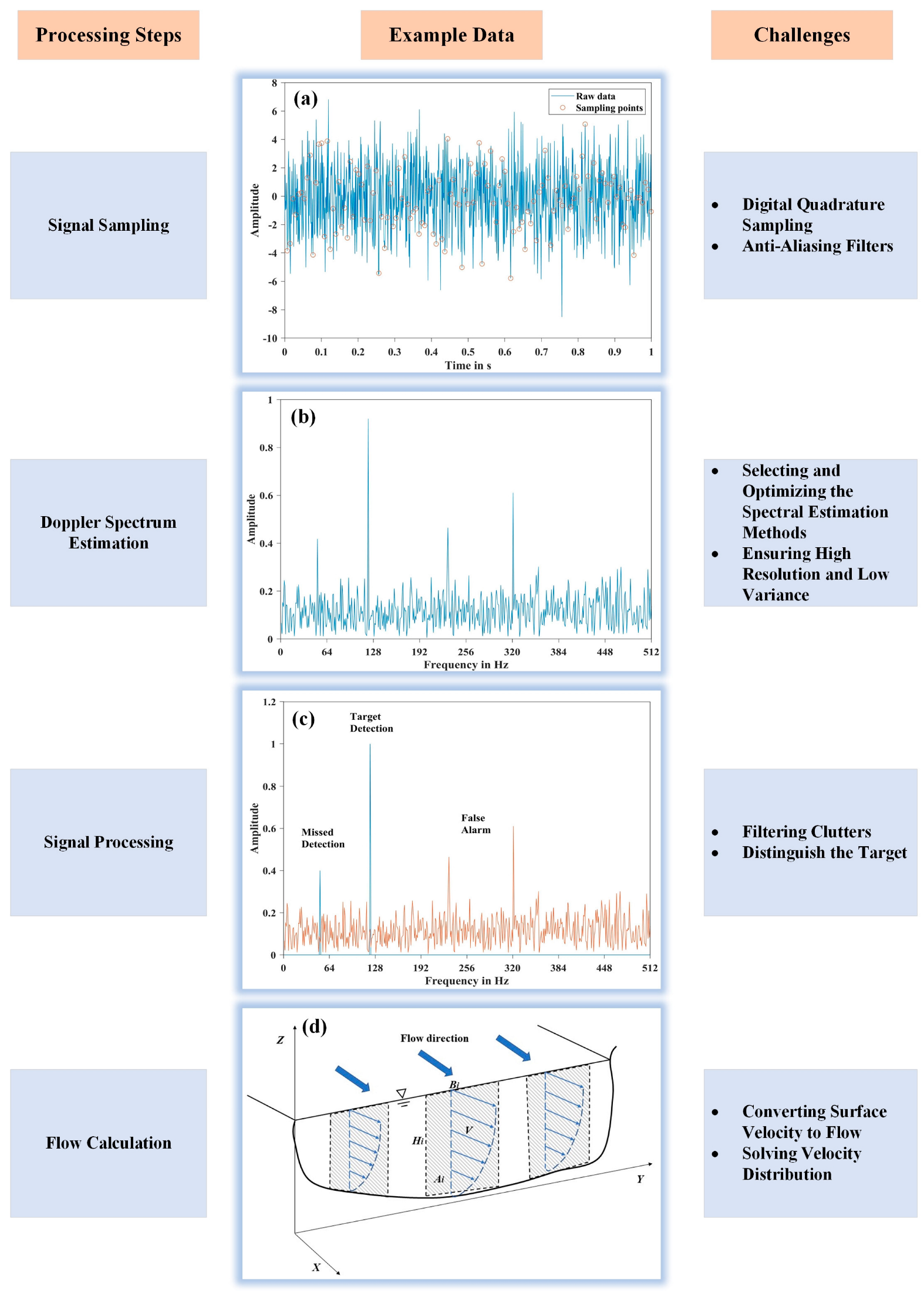
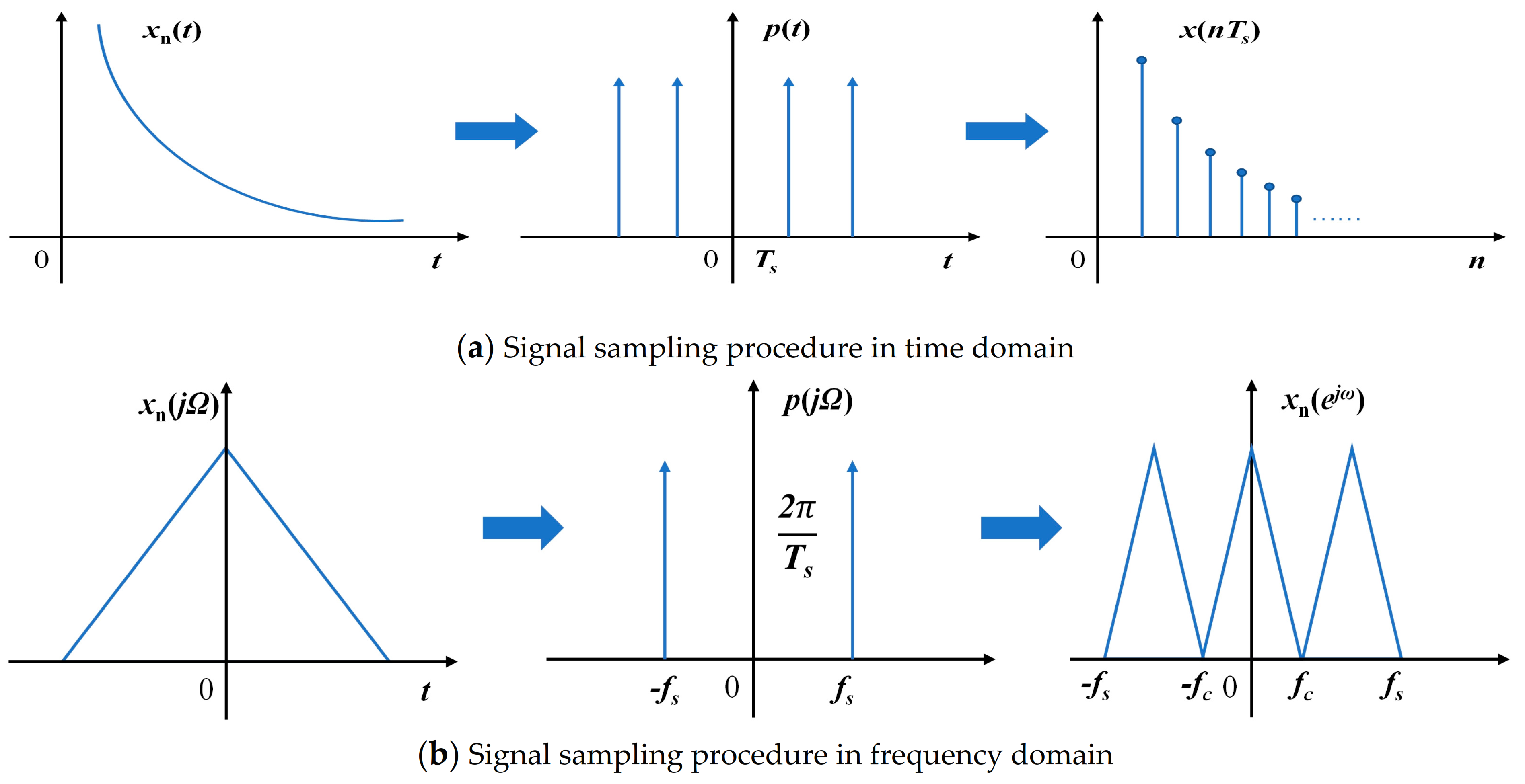
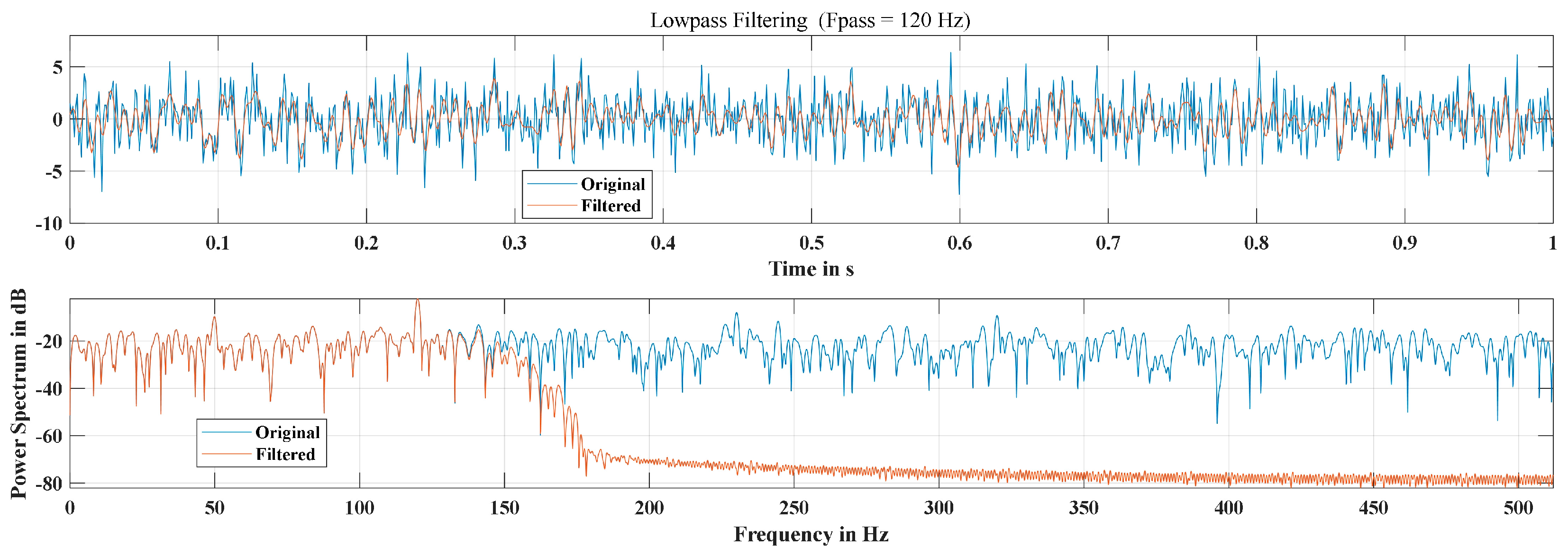
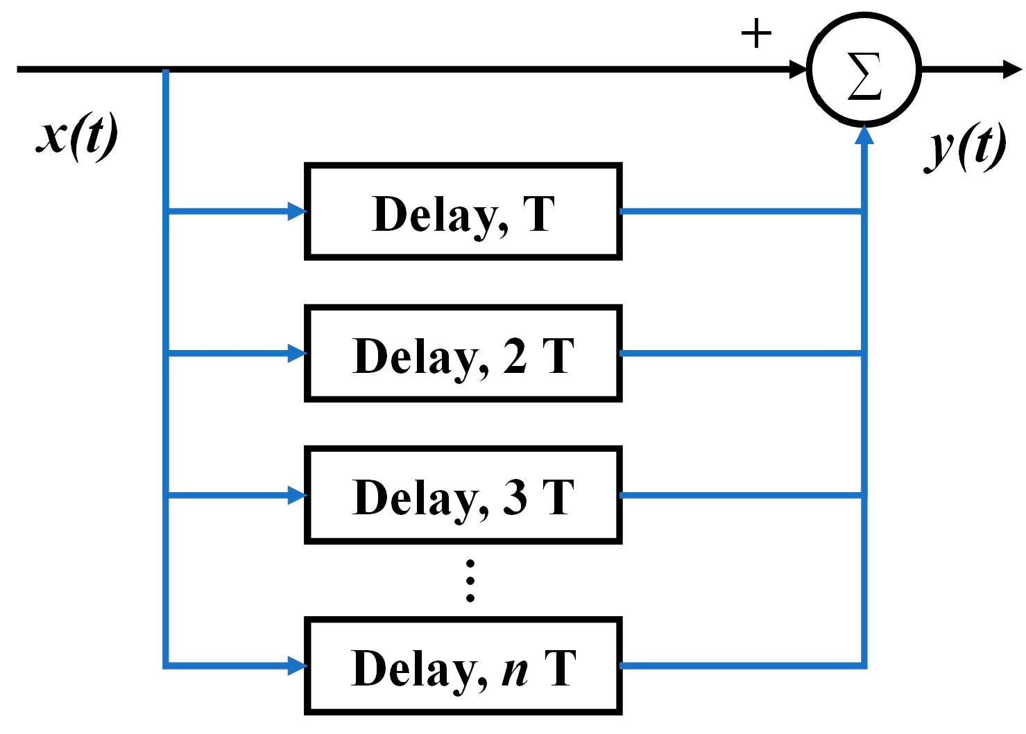
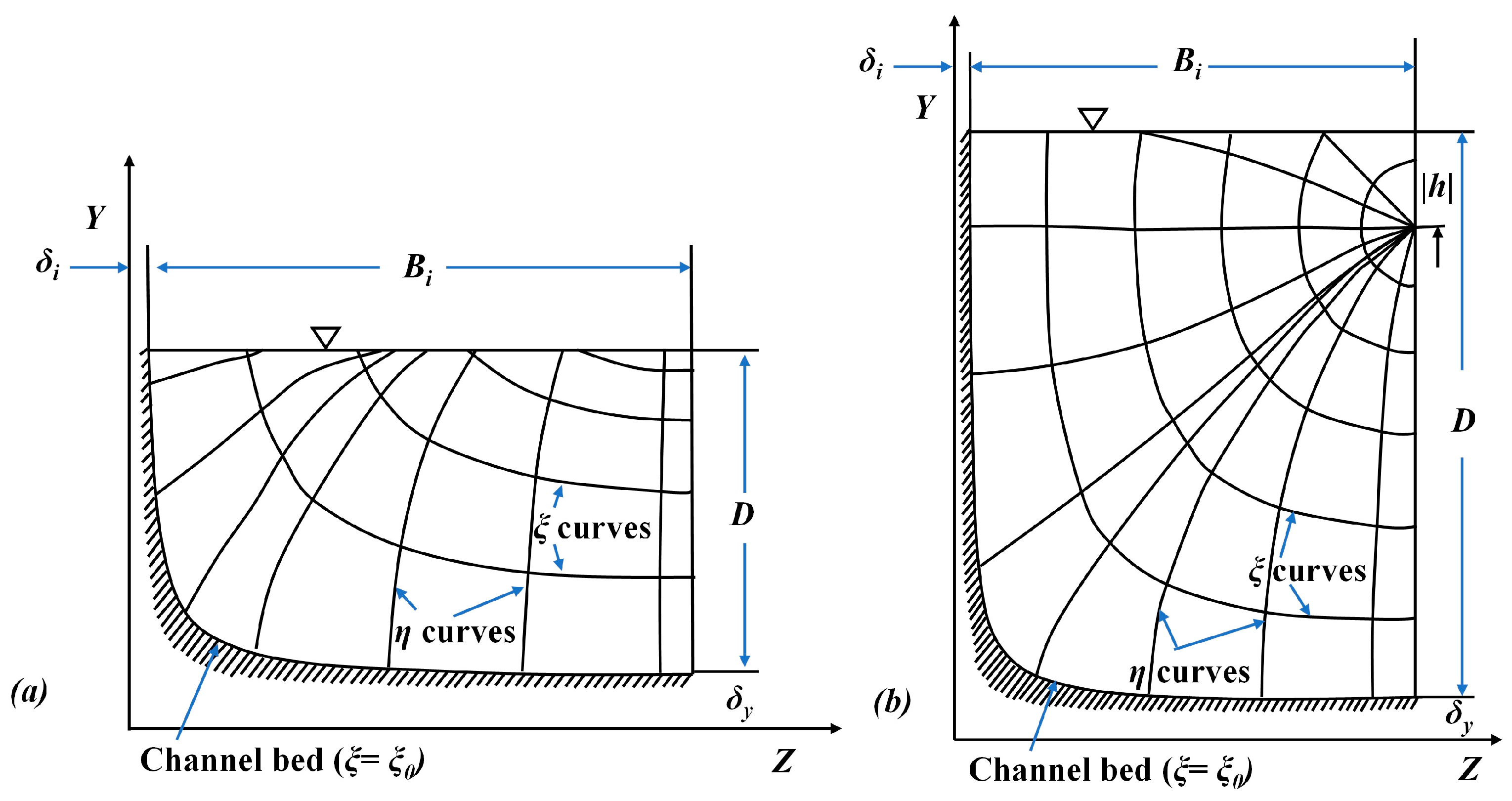
Table 1.
The advantages and disadvantages of different CFAR algorithms.
| Algorithm | Advantages | Disadvantages |
|---|---|---|
| CA-CFAR | High detection performance in the case of uniform clutter background. | The detection performance degrades in multiple targets and the clutter edge condition. |
| SO-CFAR | Good detection performance in the case of multiple targets | The probability of false alarm rises in the clutter edge condition. |
| GO-CFAR | Robust edge clutter resistance. | Multiple targets increase the likelihood of false alarms and decrease the detection performance. |
| OS-CFAR | Great detection performance in multiple targets circumstances. Good anti-clutter edge capabilities. | High false alarm loss due to the influence of k-value. Time-consuming process, and high hardware requirements. |
Table 2.
The relationship between surface velocity coefficient and channel roughness.
| Pretty Coarse | Coarse | Normal | Smooth | |
| m | 1–2 | 3–4 | 5–7 | 8–10 |
| ηs | 0.50–0.67 | 0.75–0.80 | 0.83–0.88 | 0.89–0.91 |
Disclaimer/Publisher’s Note: The statements, opinions and data contained in all publications are solely those of the individual author(s) and contributor(s) and not of MDPI and/or the editor(s). MDPI and/or the editor(s) disclaim responsibility for any injury to people or property resulting from any ideas, methods, instructions or products referred to in the content. |
© 2023 by the authors. Licensee MDPI, Basel, Switzerland. This article is an open access article distributed under the terms and conditions of the Creative Commons Attribution (CC BY) license (https://creativecommons.org/licenses/by/4.0/).
Share and Cite
MDPI and ACS Style
Huang, Y.; Chen, H.; Liu, B.; Huang, K.; Wu, Z.; Yan, K. Radar Technology for River Flow Monitoring: Assessment of the Current Status and Future Challenges. Water 2023, 15, 1904. https://doi.org/10.3390/w15101904
AMA Style
Huang Y, Chen H, Liu B, Huang K, Wu Z, Yan K. Radar Technology for River Flow Monitoring: Assessment of the Current Status and Future Challenges. Water. 2023; 15(10):1904. https://doi.org/10.3390/w15101904
Chicago/Turabian StyleHuang, Yu, Hua Chen, Bingyi Liu, Kailin Huang, Zeheng Wu, and Kang Yan. 2023. "Radar Technology for River Flow Monitoring: Assessment of the Current Status and Future Challenges" Water 15, no. 10: 1904. https://doi.org/10.3390/w15101904
Note that from the first issue of 2016, this journal uses article numbers instead of page numbers. See further details here.