Machine Learning Framework with Feature Importance Interpretation for Discharge Estimation: A Case Study in Huitanggou Sluice Hydrological Station, China

Abstract

Accurate and reliable discharge estimation plays an important role in water resource management as well as downstream applications such as ecosystem conservation and flood control. Recently, data-driven machine learning (ML) techniques showed seemingly insurmountable performance in runoff forecasting and other geophysical domains, but they still need to be improved in terms of reliability and interpretability. In this study, focusing on discharge estimation and management, we developed an ML-based framework and applied it to the Huitanggou sluice hydrological station in Anhui Province, China. The framework contains two ML algorithms, the ensemble learning random forest (ELRF) and the ensemble learning gradient boosting decision tree (ELGBDT). The SHapley Additive exPlanation (SHAP) was introduced into our framework to interpret the impact of the model features. In our framework, the correlation analysis of the dataset can provide feature information for modeling, and the quartile method was utilized to solve the outlier problem of the dataset. The Bayesian optimization algorithm was adopted to optimize the hyperparameters of the ensemble ML models. The ensemble ML models are further compared with the traditional stage–discharge rating curve (SDRC) method and the single ML model. The results show that the estimation performance of the ensemble ML models is superior to that of the SDRC and the single ML model. In addition, an analysis of the discharge estimation without considering the flow state was performed. This analysis reveals that the ensemble ML models have strong adaptability. The ensemble ML models accurately estimate the discharge, with a coefficient of determination of 0.963, a root mean squared error of 31.268, and a coefficient of correlation of 0.984. Our framework can prove helpful to improve the efficiency of short-term hydrological estimation and simultaneously provide the interpretation of the impact of the hydrological features on estimation results.

1. Introduction

The accurate estimation of discharge is important for effective water resource management and downstream ecosystem conservation. In the daily measurement tasks of the hydrological station, discharge measurement is a complex, hazardous, time-consuming, and expensive task [1,2]. Moreover, the continuous collection of discharge data is costly or impossible, especially during large flood events [3]. In general, the hydrological station provides continuous information on the water level (stage) and sparse information on corresponding discharges. Therefore, an alternative approach is to establish the stage–discharge relationship and use this relationship to convert records of the stage into discharges [4].

In previous discharge estimations, historical stage and discharge data were usually used as the basis to establish a relationship, which is known as the stage–discharge rating curve (SDRC) [5]. The quality of the SDRC determines the accuracy of the calculated discharge data. The SDRC is typically established as a single-valued relationship using statistical regression analysis of the stage and discharge measurement [6]. However, under the condition of a gentle slope and narrow channel, the discharge of a flood in the upstream phase is different from that in the downstream phase [7]. Therefore, this method cannot establish the relationship between stage and discharge under different levels of flood fluctuation. In fact, it is influenced by subjective and objective factors, such as the flood process, cross-section erosion, downstream backwater jacking, and measurement errors of the sluice gate opening height, and thus the SDRC presents a complex and non-linear relationship [8]. Obviously, the SDRC cannot describe the dynamic relationship between stage and discharge well [9]. In practical applications of the SDRC, it is necessary to consider the water flow state in the sluice waterway. In addition, the SDRC requires the establishment of multiple fitting curves, which makes it inconvenient to use.

In recent years, some ML methods, such as the decision tree, Takagi–Sugeno fuzzy inference system, neuro-fuzzy inference system (ANFIS), gene expression programming (GEP), support vector machine, back-propagation (BP) neural network, and artificial neural network (ANN) [10,11,12,13,14,15,16], have been widely used in discharge estimation and renewable energy field [17]. This is because these methods are not affected by the external physical environment. They can learn the potential correlational relationship between data to establish the quantitative relationship between input and output [18], the calculation speed is fast, and the estimation accuracy is high.

However, the decision tree, BP neural network, support vector machine, and ANN belong to a single ML. The performance of a single ML algorithm is limited, which may generate partially correct analysis results, thus reducing the reliability of the algorithm. With the rapid development and widespread application of artificial intelligence, ensemble learning [19,20] is an effective method to improve the reliability of ML algorithms. The core of ensemble learning is that the error result of a single learning machine will not affect the analysis results of most learning machines [21]. At present, two popular ensemble learning methods are bagging and boosting [22,23]. Research in many fields has shown the advantages of ensemble learning methods both theoretically and empirically [24,25]. In bagging, the basic learners are constructed using random independent bootstrap replicates from a training dataset, and the final result is calculated by means of a simple majority vote [26]. In boosting, the basic learners are constructed on a weighted version of the training dataset, which depends on the results of the previous basic learners, and the final result is calculated by means of a weighted majority vote [27,28]. Compared with a single ML algorithm, the ensemble ML algorithm trains multiple learning machines. Therefore, the ensemble ML algorithm increases the reliability and robustness of the algorithm.

Despite the success of ensemble ML, ensemble ML is visualized as a black box model, which is not highly explanatory and has no explicit physical constraints. Lack of trust in the ensemble ML is often due to a lack of interpretability [29,30]. Therefore, model interpretability is currently used to compensate for the lack of trust in models [31]. At present, the Local Interpretable Model-Agnostic Explanation (LIME) and SHapley Additive exPlanation (SHAP) are the most popular explainable methods [32,33]. Among them, the LIME method interprets individual model estimations based on linear assumptions and locally approximates the model around a given estimation [32]. However, the explanations are very unstable [34]. For most of these explanatory solutions, an important goal is to answer which input features are more important to the output of the model [35]. One prominent example is the SHAP method. The SHAP method is derived from Shapley values in game theory, which describe the contribution of each team member in a collaborative environment [36]. In ML, it works by assigning important values to each feature for a particular estimation. In addition, Microsoft researchers have published a unified interpretive framework for ML [33].

The main research objectives of this work were as follows: (1) to focus on discharge estimation and management, by developing an ML-based framework; (2) to interpret the impact of the model features, by introducing the SHAP into our framework; (3) to verify the effectiveness and applicability of the proposed method in discharge estimation, by conducting the method in a real-world case study at Huitanggou sluice hydrological station in Anhui Province, China. The correlation analysis of the dataset can provide feature information for modeling, and the Bayesian optimization algorithm was adopted to optimize the hyperparameters of the ensemble ML models. This approach can be utilized to estimate the discharge of the sluice hydrological station and further transfer application to other similar domains.

2. Methodology

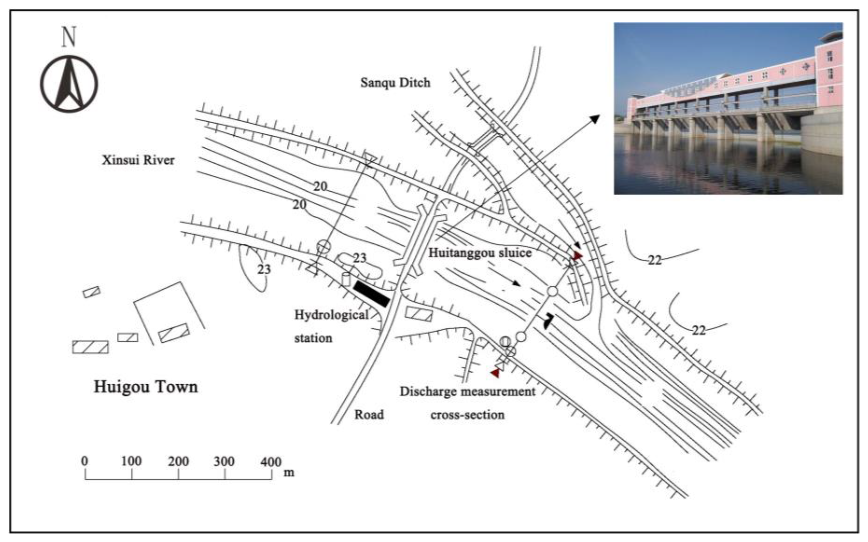
2.1. Study Area and Data Sources

Huitangguo sluice hydrological station, an important control station to the Xinsui River in Suzhou city, Northern Anhui Province, China, is shown in Figure 1. The hydrological station is located at longitude 117°33′59″ E, latitude 33°45′26″ N. The watershed encompasses an area of 2396 square kilometers. Huitangguo sluice hydrological station was established in 1951. The measurement items include stage, discharge, precipitation, evaporation, groundwater, soil moisture, and water quality. Huitanggou sluice was demolished in 2006 and moved upstream for reconstruction. The discharge measurement cross-section was also moved to above the Sanqu ditch estuary. The new sluice (Figure 2) has a total of 7 waterways and every waterway is 12 m wide. The type of sluice gate is arc-shaped, and the composition consists of steel. The elevation of the sluice bottom is 16.18 m.

Many variables can affect discharge estimation. After the analysis of the actual situation of the Huitangguo sluice hydrological station, the data of six variables were selected. The variables Z_u, Z_d, e, n, B_q, and A_q are the upstream stage, downstream stage, sluice gate opening height, sluice gate opening number, discharge measurement cross-section width, and discharge measurement cross-section area, respectively. Among them, the measurement position of Z_u was 120 m away from the upstream of the sluice, and the measurement position of Z_d was 380 m away from the downstream of the sluice. In total, 1281 sets of Z_u, Z_d, e, n, B_q, A_q, and measured discharge (Q_m) data covered the period from 2008 to 2022. The dataset was divided into the training set and the testing set at a ratio of 7:3. The measured data were derived from the Suzhou Hydrology and Water Resources Bureau of Anhui Province. The descriptive statistics of these variables are summarized in

Table 1. Summary of descriptive statistics for variables.

Dataset	Number of Cases	Variable	Minimum	Maximum	Mean	Median	Standard Deviation
Training	897	Zu (m)	17.07	23.06	21.13	21.31	0.81
		Zd (m)	16.77	22.97	18.26	18.16	0.87
		e (m)	0.10	6.86	0.52	0.30	0.89
		n	1	7	3	2	2
		Bq (m)	97.5	158	118.1	119	7.1
		Aq (m2)	28.1	856	200.7	188	109.1
		Qm (m3/s)	2.49	875	66.9	36.6	107.4
Testing	384	Zu (m)	18.43	22.96	21.15	21.27	0.69
		Zd (m)	17.08	22.92	18.52	18.18	1.20
		e (m)	0.10	6.76	0.91	0.30	1.55
		n	1	7	3	2	2
		Bq (m)	89.1	156	120.8	121	8.9
		Aq (m2)	63.5	818	241.9	195	153.3
		Qm (m3/s)	7.75	767	116.9	45.6	163.3

. The variation amplitude of Q_m and A_q was higher than that of Z_u and Z_d. The minimum and maximum values of Z_u, Z_d, A_q, and Q_m in the testing set fell within the range in the training set. This shows that the training set with a wider data spectrum can guarantee a robust model for estimating discharge in a wider range, and can overcome the problem of estimating extreme discharge values.

2.2. Methods

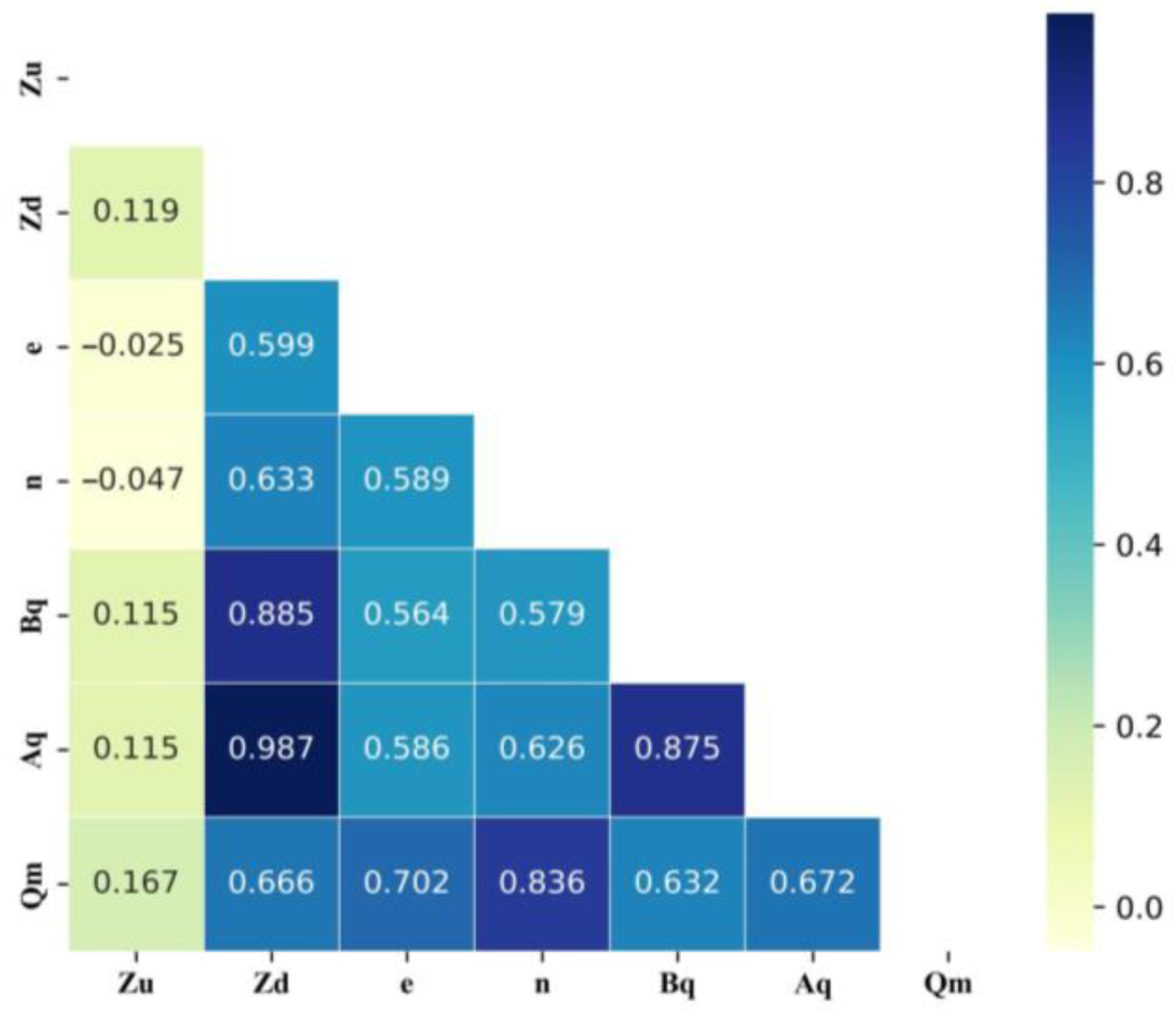
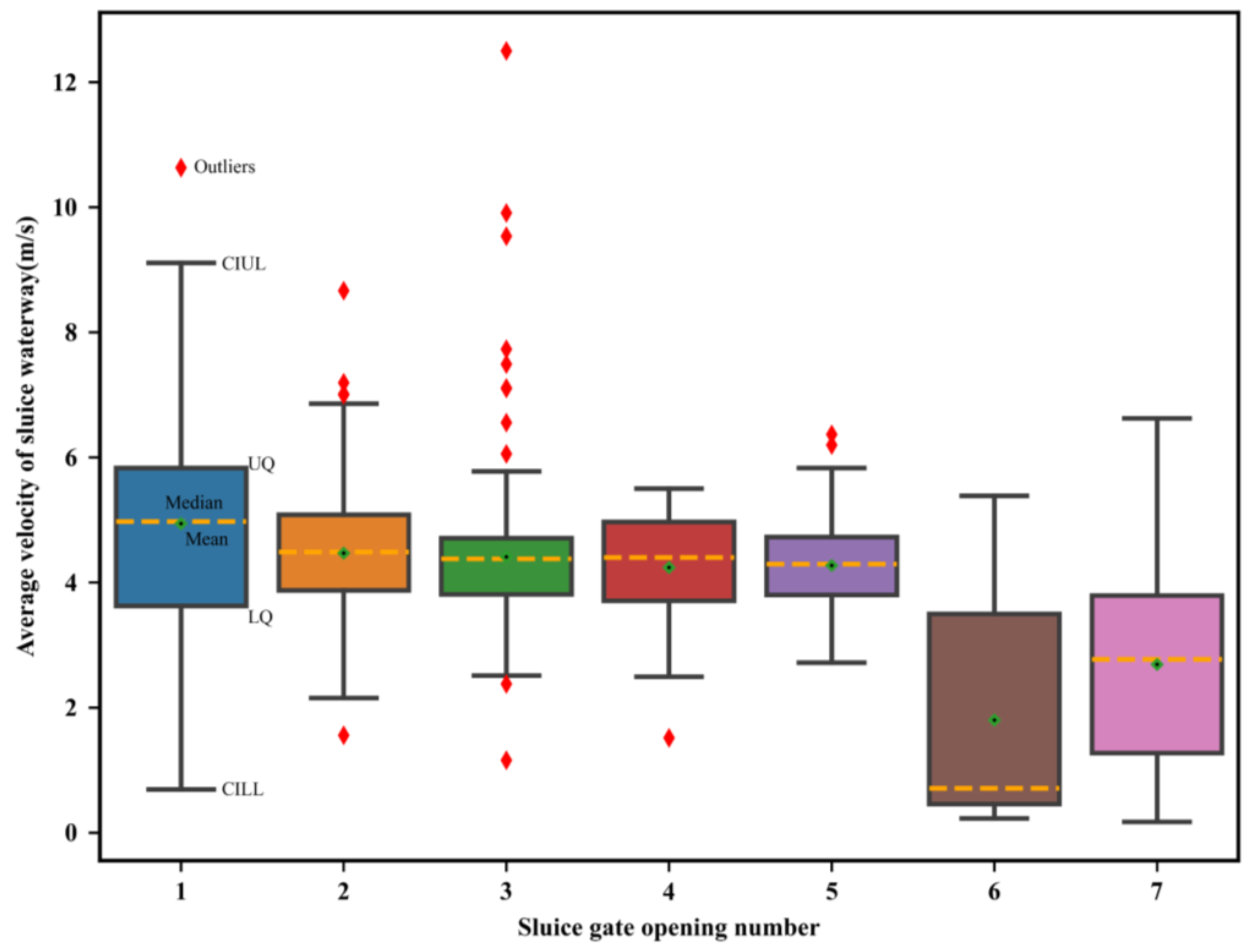
2.2.1. Exploratory Data Analysis (EDA)

EDA is helpful for finding the outliers of the dataset and providing a reference for modeling, which can improve the estimation accuracy of the model. In this study, Spearman’s rank correlation coefficient (SRCC) (Equations (1) and (2)) [37] was used to find the features that have a weak correlation relationship with discharge. The quartile method [38] was applied to solve the outlier problem of the dataset. The quartile method is a statistical descriptive analysis method used to describe various types of data. Itis one of the most common methods used to detect outliers. This method uses the median to measure the trend in concentration of the data and the quartile interval to measure the dispersion of the data, because these statistics are more robust to outliers.

$$a=\sum _{i=1}^n{\left|f\left(x_i\right)-f\left(y_i\right)\right|}^2$$

(1)

$$SRCC=1-\frac{6a}{n(n^2-1)}$$

(2)

where $f\left(x\right)$ and $f\left(y\right)$ are the ranks of variables $x$ and $y$, respectively, and n is the number of samples.

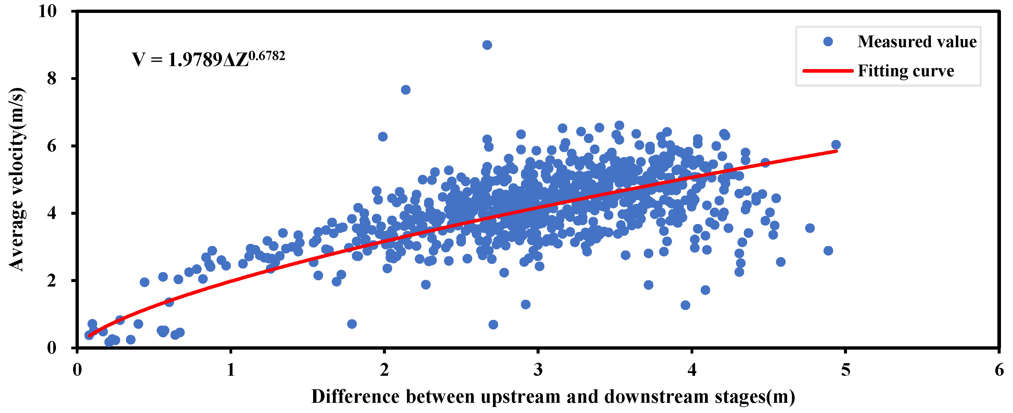
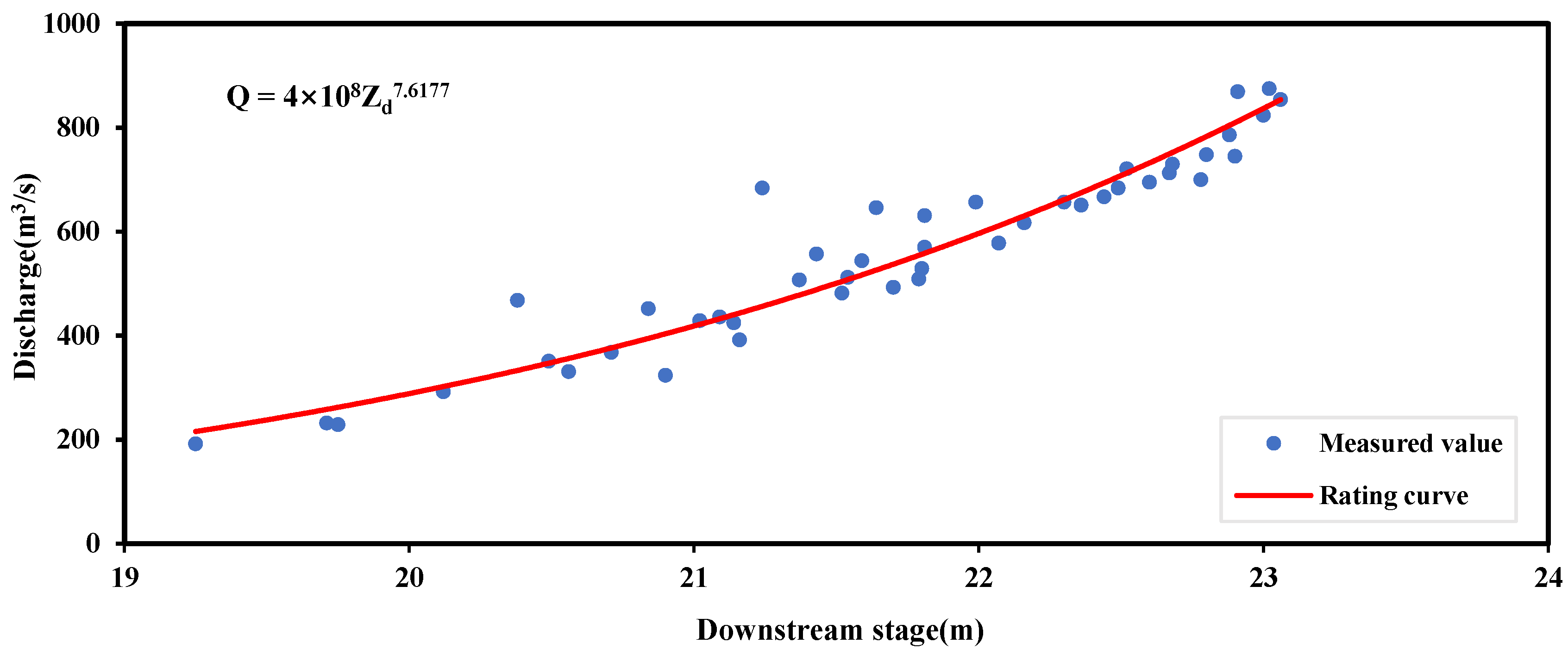
2.2.2. Conventional Method: Stage–Discharge Rating Curve (SDRC)

The SDRC is a useful tool for a hydrologist to estimate discharge from gauge observations. It alleviates the need for costly and time-consuming discharge measurements [16]. The Huitanggou sluice is affected by the water storage of the downstream sluice, and it has always demonstrated the submerged orifice flow state and the submerged weir flow state. According to the principle of hydraulics, the average velocity of the sluice waterway is mainly related to the difference between the upstream stage and downstream stage in the submerged orifice flow state (Equations (3) and (4)), and the discharge is mainly related to the downstream stage in the submerge weir flow state (Equation (5)). In hydrology, many observations of stage and discharge data are often used to calibrate the relationship formula or relationship curve between stage and discharge, which is used to estimate the discharge, reduce the intensity of measurement and improve the accuracy of the calculation.

$$V_i=a{∆Z}_i^b,i=\mathrm{1,2},3\dots ,n$$

(3)

$$Q_i=Be{V}_i,i=\mathrm{1,2},3\dots ,n$$

(4)

$$Q_j=m{Z}_{dj}^t,j=\mathrm{1,2},3\dots ,n$$

(5)

where $V_i$ is the average velocity of sluice waterway; ${∆Z}_i$ is the difference between the upstream stage and downstream stage; $B$ is the sluice gate opening total width; e is the sluice gate opening height; $Z_{dj}$ is the downstream stage; a, b, m and t are the coefficients; $Q_i$ is the submerged orifice discharge; and $Q_j$ is the submerged weir discharge.

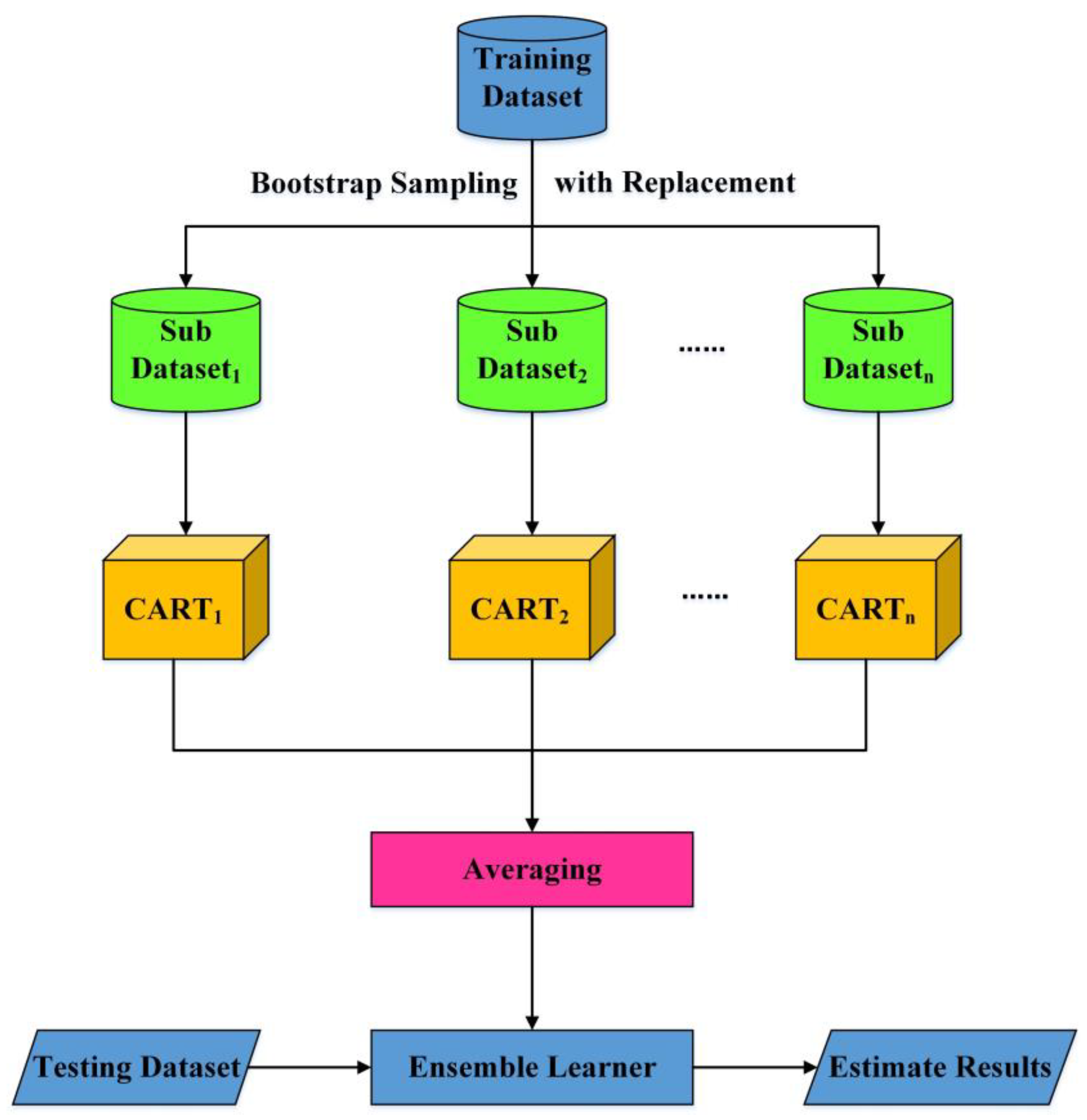
2.2.3. Ensemble Learning Random Forest (ELRF) Algorithm

The ELRF algorithm [39] is a typical bagging algorithm which is widely used in finance, medicine, manufacturing, and other fields. The basic principle is to extract several subsets from the original training set according to the Bootstrap method. Then, different features are extracted, and the base model is trained on different subsets. The Bagging algorithm generates multiple training sets by extracting training samples and training a classification and regression tree (CART) [40] on a subset of each training set. The results of multiple CART are arithmetically averaged to produce the final result [41]. The random forest (RF) algorithm is an ML algorithm with higher accuracy. The RF algorithm adopts CART as the base model. The CART is widely used in regression problems. It uses impurity as the basis for its tree model segmentation. This paper studies a regression problem, so the mean square error (MSE) is selected as the impurity function. Figure 3 exhibits the bagging algorithm process.

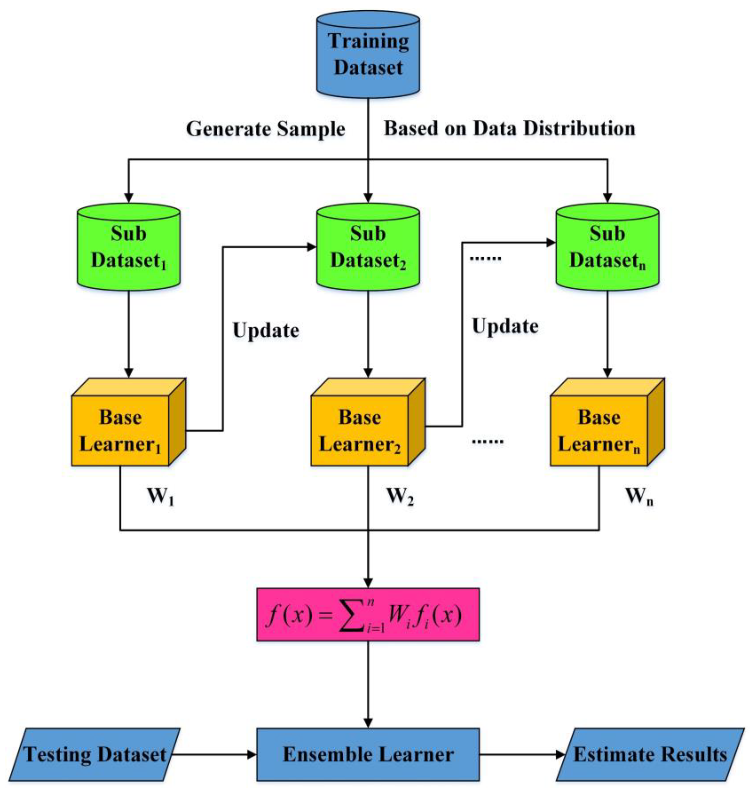
2.2.4. Ensemble Learning Gradient Boosting Decision Tree (ELGBDT) Algorithm

The ELGBDT algorithm is a classic boosting algorithm, which is a decision tree model of sequence ensemble learning (Figure 4). In each round of model training, each calculation of gradient boosting seeks to reduce the residual error generated by the previous decision tree. This causes the overall model to have better data fitting ability and improves the training effect of the model [42]. In the iterative process of the model training of the gradient boosting decision tree (GBDT) algorithm, as the number of individual learners increases, the value of the loss function decreases significantly [43]. The loss function of the GBDT algorithm is as follows:

$$L\left(y_i,f_i\left(x\right)\right)=L\left(y_i,f_{i-1}\left(x\right)+h_i\left(x\right)\right)$$

(6)

$$L\left(y_i,f_i\left(x\right)\right)<L\left(y_i,f_{i-1}\left(x\right)\right)$$

(7)

$$F\left(X\right)=\mathrm{m}\mathrm{i}\mathrm{n}\sum _{i=1}^{n}L\left(y_i,f_i\left(x\right)\right)$$

(8)

where $f_{i-1}\left(x\right)$, $L\left(y_i,f_i\left(x\right)\right)$, $h_i\left(x\right)$, $y_i$ and $n$ are the strong learners from the fusion of individual learners in the $i-1$ rounds, the loss function in the $i$ rounds, the base learners in the $i$ rounds, the measured values, and the number of base learners, respectively.

In this study, the base learner was the CART. The training process can be divided into the following steps: (1) the multiple training sets were generated, and the weight initialization of the training set ($W_i$, $i$ = 1, 2, …, $n$) was conducted. The first weak base learner (BL₁) was trained based on W₁, and the weight of BL₁ was updated based on its learning performance. The poorly performing data from BL₁ were recorded and their weights were set higher in W₂ to make them more important to BL₂. (2) The BL₂ was trained based on the knowledge from the previous step, and this iteration continued until the number of learning machines reached the set number. In this study, the number of learning machines was set to 100. (3) Based on ensemble learning, by integrating multiple learning machines into a machine learning algorithm, we obtained a machine learning algorithm with greater generalization ability.

2.2.5. SHAP Algorithm

SHAP is an explanatory model of additivity constructed by Lundberg [33] in 2017, inspired by cooperative game theory (Figure 5). The core of the algorithm is to calculate the SHAP values (Equation (9)). SHAP values can reflect the contribution of features to the estimation ability of the overall model. SHAP interprets the estimated value of the model as the sum of the SHAP values of each input feature. SHAP provides not only the contribution of each feature to the whole ML model, but also the positive and negative impact of each feature value in each sample point on the estimation result [44]. For each estimation sample, the model generates an estimation value, and the SHAP values are the numerical values assigned to each variable in that sample. The SHAP method reveals the interactions between all variables and how this relationship is reflected in the model. Therefore, the SHAP is beneficial for increasing the interpretability of the model, thereby increasing trust in the model.

In ML interpretable methods, the traditional method of feature importance will be affected by noise and feature interference with high correlation, and these problems can be solved by the SHAP method. In addition, the traditional method of feature importance can directly reflect the importance of features, but cannot determine the relationship between features and the final estimation result. SHAP uses the feature attribution method to calculate the attribution value of features, which can reflect the impact of each feature on the final estimated value, increasing the interpretability of the model. SHAP can be applied to any ML model, especially in the ensemble learning model based on the decision tree, which can have higher efficiency and richer interpretation functions. Moreover, the SHAP provides a powerful data visualization function to display the interpretation results of models and estimations and is widely used to interpret more complex algorithm models.

$$y_i=\stackrel{-}{y_0}+f\left(x_{i1}\right)+f\left(x_{i2}\right)+\dots +f\left(x_{in}\right)$$

(9)

where $y_i$, $\stackrel{-}{y_0}$, $x_{in}$, and $f\left(x_{in}\right)$ are the estimated value, the mean of the target variable, the feature of $n$ in the $i$ sample, and the SHAP value of $x_{in}$, respectively.

2.2.6. Bayesian Optimization Algorithm

The Bayesian optimization algorithm is an automatic parameter tuning algorithm based on the Gaussian process [45,46]. Due to its ability to quickly obtain the optimal value, it is widely used in the field of computer science to determine the optimal hyperparameter values of models [47]. Compared with the grid search parameter tuning method, the Bayesian optimization algorithm has fewer iterations and faster speed. The acquisition function (Equation (10)) is used to set the update and measure the expected utility of performing an evaluation of the objective at the new point. In this study, the objective function is root mean squared error.

$$x=\underset{x\in X}{\min }f\left(x\right)$$

(10)

where $f\left(x\right)$, $x$, and $X$ are the objective function to be optimized, the next acquisition point of Bayesian optimization, and the search space of the target solution, respectively.

2.3. Performance Evaluation Methods

In this study, four standards were used to validate the performance of the models to avoid the limitation of a single evaluation standard. The coefficient of determination (R²), root mean squared error (RMSE), coefficient of correlation (CC), and relative error (RE) (Equations (11)–(14)) were used as the evaluation standards. They, respectively, represent the fitting degree, relative deviation degree, correlation degree between estimated values and measured values, and the stability of models.

$$R^2=1-\frac{\sum {\left(Q_m-Q_p\right)}^2}{\sum {\left(Q_m-{\stackrel{-}{Q}}_m\right)}^2}$$

(11)

$$RMSE=\sqrt{\frac{\sum {\left(Q_m-Q_p\right)}^2}{n}}$$

(12)

$$CC=\frac{\sum (Q_m-{\stackrel{-}{Q}}_m)(Q_p-{\stackrel{-}{Q}}_p)}{\sqrt{\sum {(Q_m-{\stackrel{-}{Q}}_m)}^2\sum {(Q_p-{\stackrel{-}{Q}}_p)}^2}}$$

(13)

$$RE=\left|\frac{Q_m-Q_p}{Q_m}\right|$$

(14)

where $Q_m$ and $Q_p$ are the measured discharge values and the estimated discharge values, respectively; ${\stackrel{-}{Q}}_m$ and ${\stackrel{-}{Q}}_p$ are the average value of $Q_m$ and the average value of $Q_p$, respectively; and $n$ is the length of dataset.

3. Results

3.1. Data Exploration and Analysis

The analysis of error or uncertainty in model estimation is very useful for modeling. In this study, the source of error is mainly caused by variable measurement. After obtaining the dataset, this research first performed EDA. EDA can discover laws from the dataset, the correlation analysis of the dataset can provide a reference for modeling, and the quartile method can find the outliers of the dataset. Figure 6 shows the SRCC heatmap of the six variables and measured discharge. As can be seen in Figure 6, the six variables have different degrees of positive correlation with the measured discharge. Among them, the correlation degree of Z_u and Q_m is the weakest, and the correlation degree of n and Q_m is the strongest. Except for Z_u, the absolute value of SRCC between the variables and Q_m is greater than 0.5, which indicates that the selected variables have a high correlation with Q_m. Therefore, the input variables for the ELRF and ELGBDT models include Z_u, Z_d, e, n, B_q, and A_q.

Figure 7 presents box plots of the average velocity of the sluice waterway (V). The top horizontal line segment represents the confidence interval upper limit (CIUL) of the V distribution, the upper, middle, and lower line segments of the box represent the upper quartile (UQ), median, and lower quartile (LQ) of the V distribution, and the bottom line segment represents the confidence interval lower limit (CILL) of the V distribution. The red dots represent the outliers of the V distribution, and the black dot represents the mean value of the V distribution. As can be seen from the box plots, except for waterways six and seven, all of the waterways have abnormal points. So, the models developed in this study after the data were cleaned through the quartile method. The number of samples after data cleaning is 1256 sets.

3.2. Conventional SDRC Fitting

The functional relationship between stage and discharge can be established by the measured values of the stage, sluice gate opening height, sluice gate opening number, and discharge. The fitting curve is shown in Figure 8 and the rating curve is shown in Figure 9.

As can be seen from Figure 8, the estimated average velocity of the sluice waterway (V) remained within a reasonable range of the measured values for most of the time. However, the V values from the rating curve showed great variation from the measured values in some cases. Because the SDRC bears certain non-idealized features, such as section erosion, downstream backwater jacking, measurement error of the sluice gate opening height, the SDRC presents a non-linear relationship. Therefore, the fitting effect of the SDRC is poor. Figure 9 shows the SDRC of the submerged weir flow state. Because of the small sample size of the dataset, most of the points are distributed on the red line, and the SDRC is prone to overfitting.

3.3. Model Estimation

3.3.1. Bayesian Hyperparameter Optimization

The hyperparameter tuning of the model is a significant work. In this study, the optimal hyperparameters were determined using the Bayesian optimization algorithm. The Bayesian tuning uses a Gaussian process, which considers the previous parameter information and constantly updates the prior [45]. It has fewer iterations and faster speed. The Bayesian tuning is still robust for non-convex problems, so the model has good generalization ability. The number of iterations is 30, and the optimal target values for the ELRF and ELGBDT models in the submerged orifice flow state are 0.931 and 0.929, respectively. In this study, the optimal target values are the optimal coefficient of determination values for the ELRF and ELGBDT models. The optimization process for the hyperparameters of ELRF and ELGBDT models is presented in Tables S1 and S2 in the Supplementary Materials, respectively.

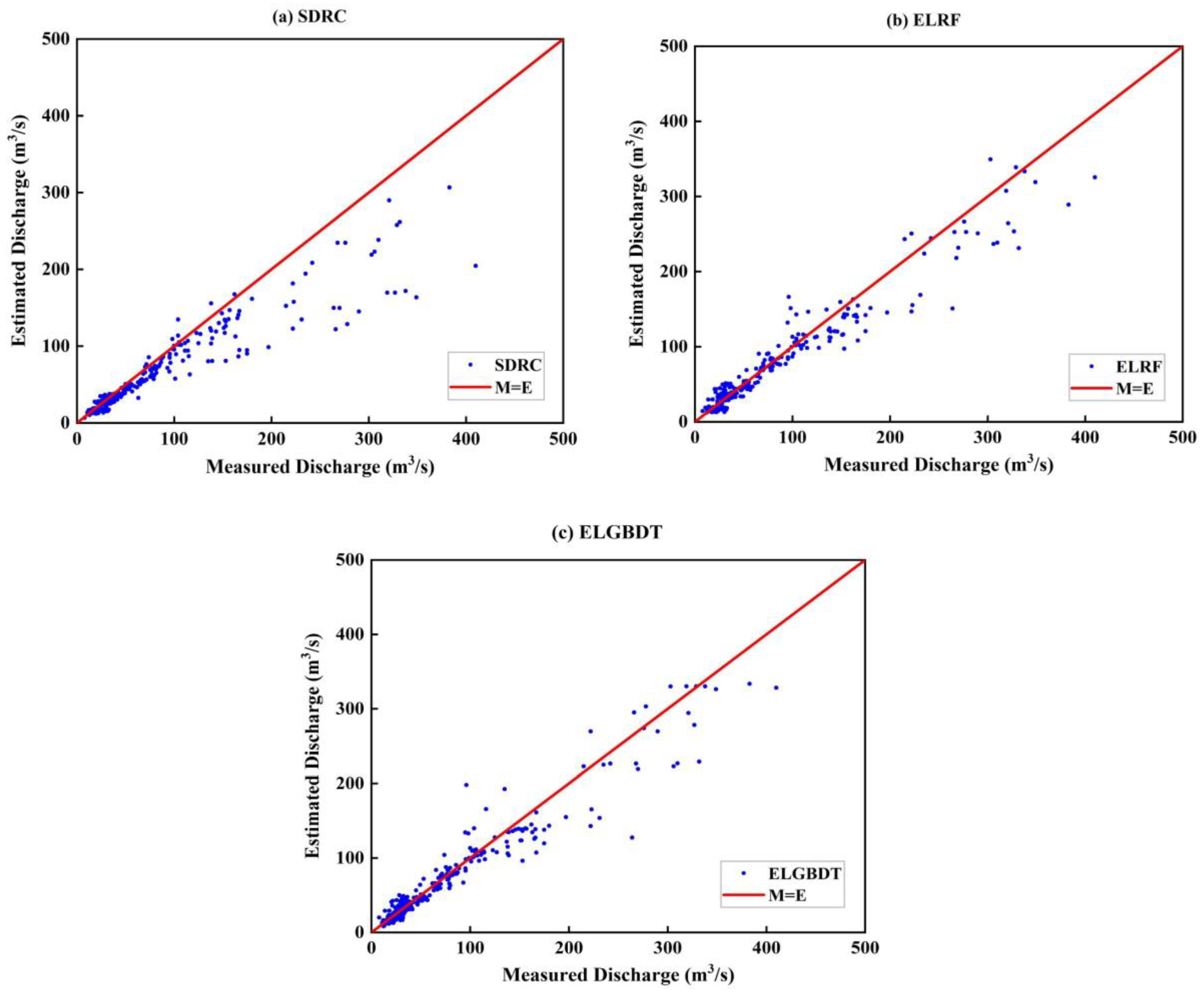
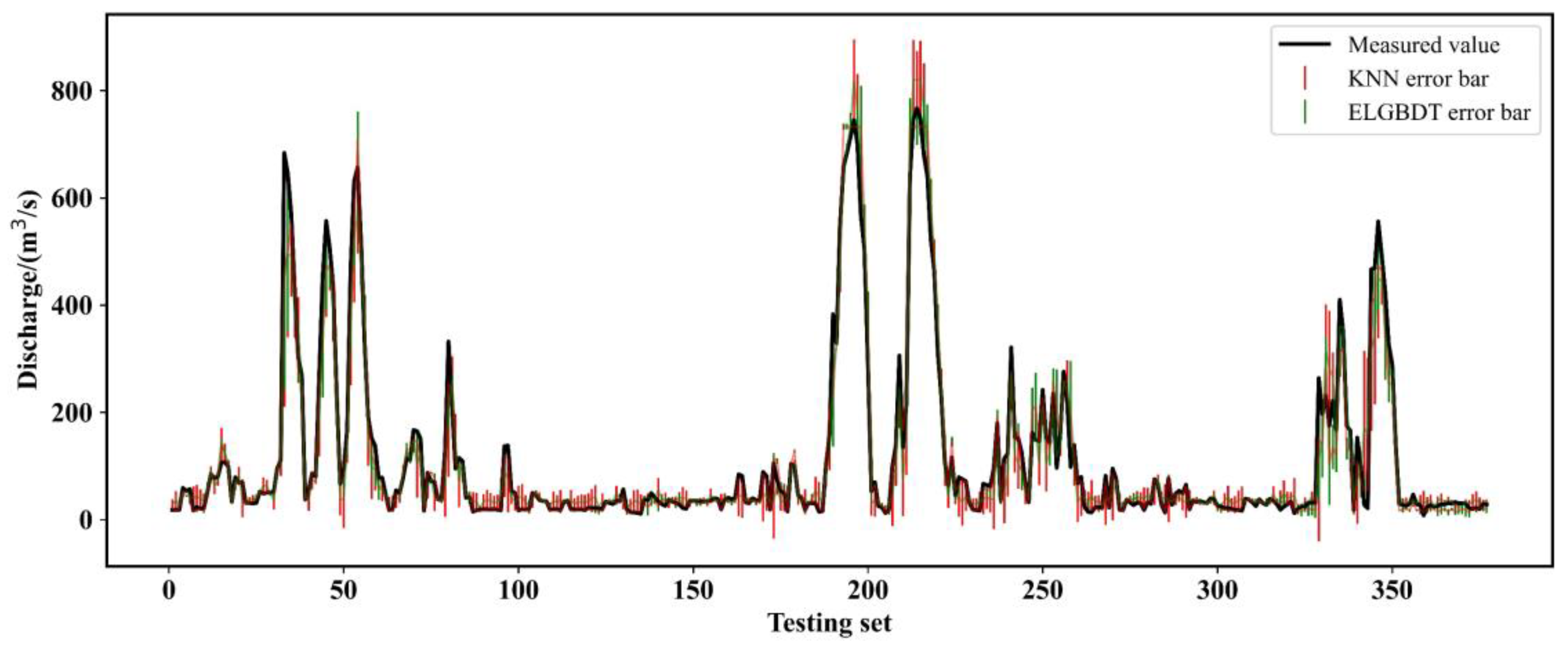
3.3.2. Model Evaluation

Table 2. Estimated results of the submerged orifice flow state.

Model	R2	RMSE	CC
SDRC	0.801	33.354	0.947
ELRF	0.911	19.578	0.971
ELGBDT	0.912	19.955	0.967

presents the estimated results of the submerged orifice flow state after Bayesian optimization. Due to the small sample size in the submerged weir flow state, three models are prone to overfitting, and the generalization ability of the models is weak. So, they are not displayed. From Table 2, it can be seen that the overall performance of the model developed using ELRF and ELGBDT is better than that of the SDRC model. According to the three evaluation standards, the R², RMSE, and CC values of the ELRF are similar to those of the ELGBDT model. This indicates that the ELRF and ELGBDT models estimate discharge with almost identical accuracy. The R² of the ensemble ML model increased by 13.86% compared to that of the SDRC model. This shows that the fitting degree of the ensemble ML model is high. The RMSE of the ensemble ML model is 41.30% lower than that of the SDRC model. This reveals that the stability of the ensemble ML model has strong. The CC of the ensemble ML model increased by 2.53% compared with the SDRC model. It can be seen that the correlation degree of the ensemble ML model is high. Therefore, the ensemble ML model has a stronger learning ability.

Figure 10 compares the estimated discharge distribution of the three models. As detailed in Figure 10, the distribution of SDRC model dots is mostly below the red line. This shows that the estimated discharge of the SDRC model is lower. The distribution of the other two model dots is even and similar. This reveals that the ensemble learning model performs well where both high and low discharges were reasonably estimated. Meanwhile, the stability of the models is validated by the RE between each estimated discharge and measured discharge. The violin plots of the three models are shown to compare the RE distributions. Figure 11 and

Table 3. RE distribution parameters of three models.

Model	CIUL (%)	UQ (%)	Median (%)	LQ (%)	CILL (%)
SDRC	52.90	25.80	14.02	7.74	0
ELRF	50.07	24.54	13.50	7.53	0
ELGBDT	49.38	24.25	14.81	7.49	0

Note: CIUL is the confidence interval upper limit; UQ is the upper quartile; LQ is the lower quartile; CILL is the confidence interval lower limit.

shows the violin parameters.

Figure 11 details the violin plot of the three models after removing outliers greater than 1. As detailed in Table 3 and Figure 11, the RE distribution of the ELRF and ELGBDT models is similar. Compared with the violin parameters of the SDRC model, although the CILL of the ensemble ML model and SDRC model are both 0, the violin parameters of the ensemble ML model have a smaller CIUL, UQ, median and LQ. The 95% confidence interval (CI) and interquartile range (IQR) of the ensemble ML model are smaller than that of the SDRC model. Therefore, the stability of the ensemble ML model is better.

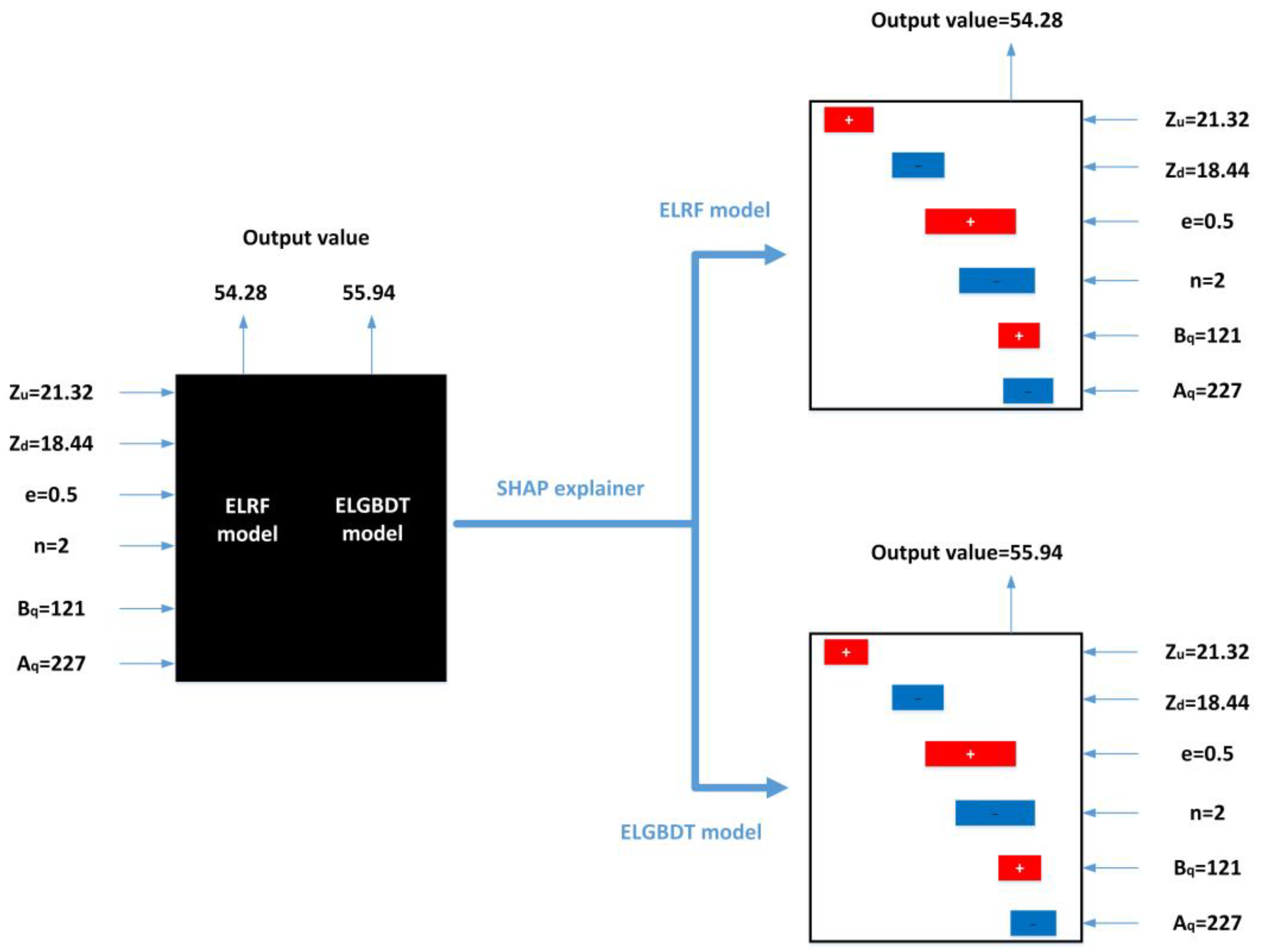
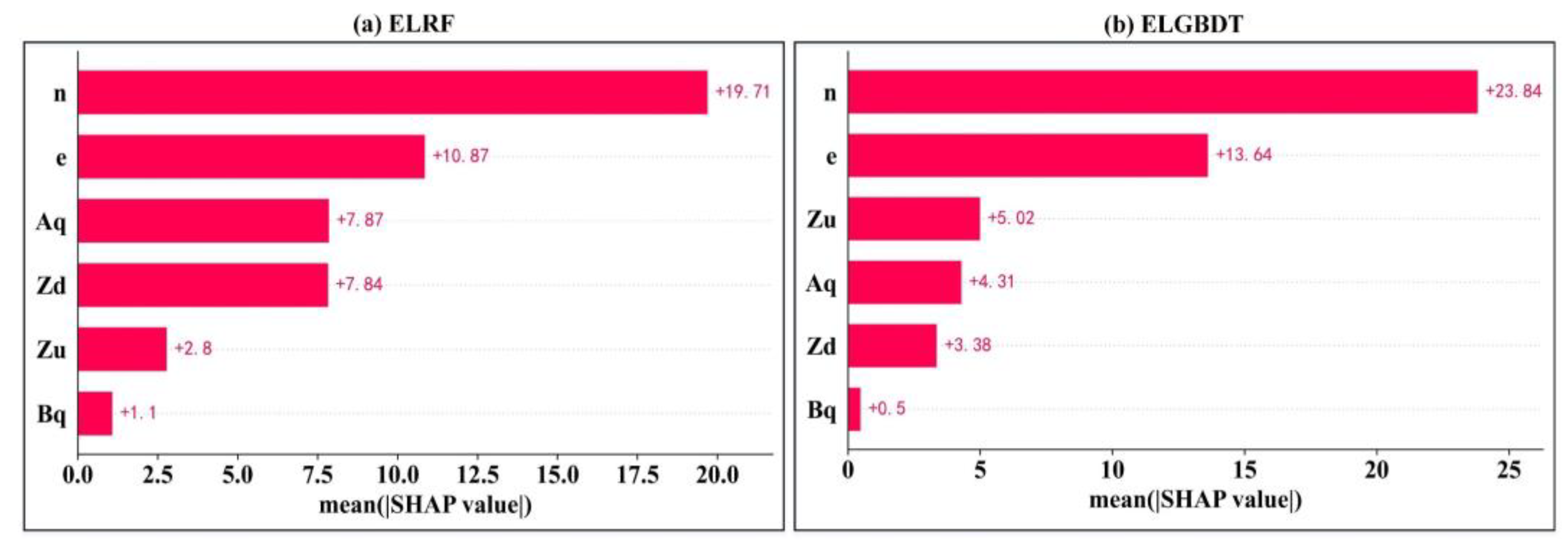
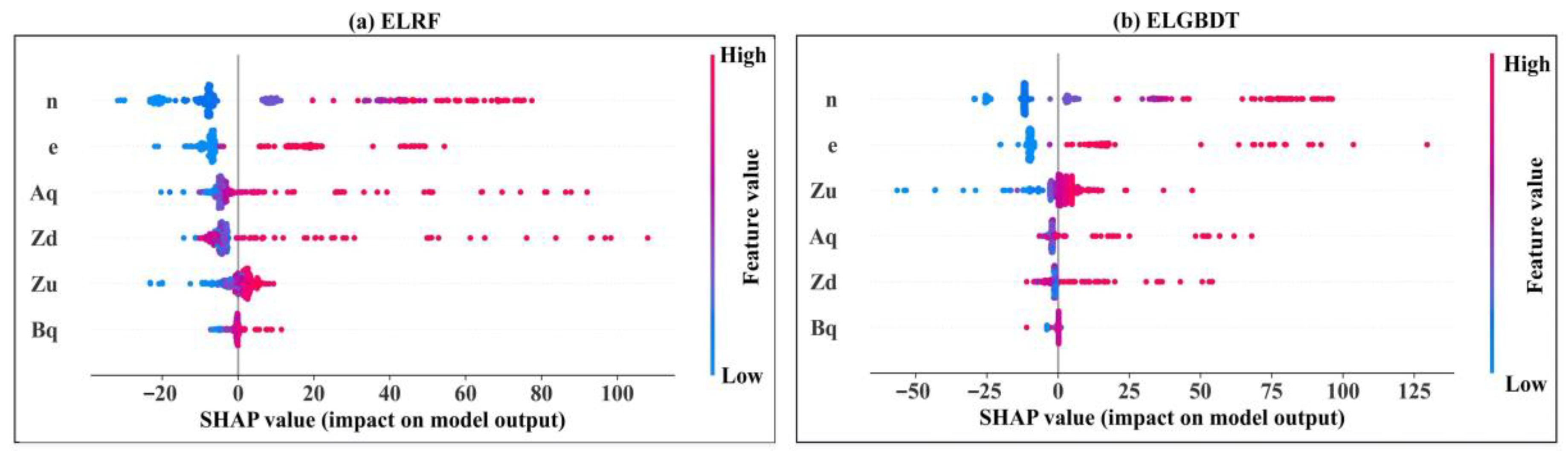
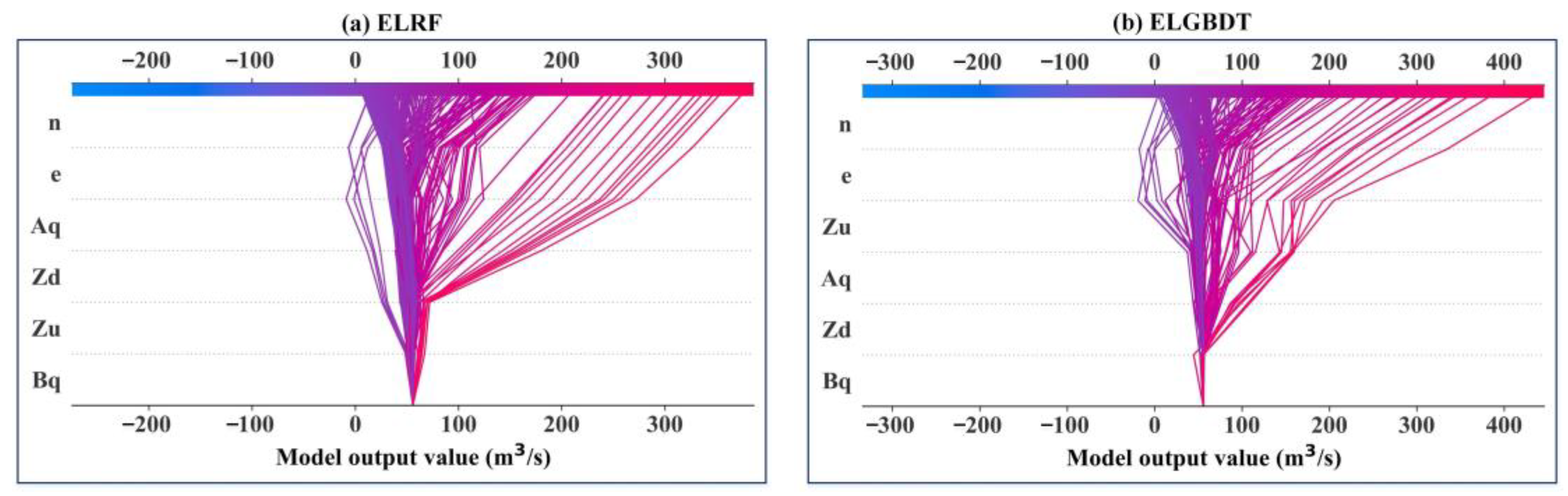
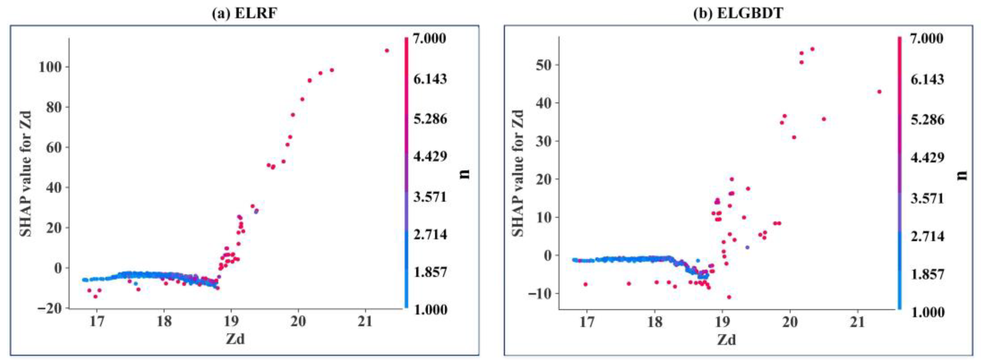
3.4. Model Feature Importance Interpretation

To determine the contribution of each variable, Figure 12 represents an absolute summary plot where the mean value of the SHAP values for each variable is used to obtain a bar chart as a function of the contribution of each variable to the estimation of the ELRF and ELGBDT models. From this plot, it can be inferred that the influential variables of the two models are different. For example, the most influential variables in the ELRF model are n, e, and A_q, from greater to lesser significance, respectively (Figure 12a). In the ELGBDT model, the influential variables from strong to weak are n, e, Z_u, A_q, Z_d, and B_q, respectively (Figure 12b).

Figure 13 represents a summary plot that shows the contribution of each variable to the ELRF and ELGBDT models, taking into account all values of each variable. The figure includes all of the variables of the input model, where the magnitude is indicated by the colored line on the right. As can be seen from Figure 13, the summary plots of the two models are similar. The summary plot shows that the existence of the variable n (higher values in red on the horizontal bar) means an increase in the estimated discharge (indicated on the scale at the bottom of the figure); in contrast, the lack of n (lower values in blue on the horizontal bar) is associated with a decrease in the estimated discharge. The same analysis can be applied to the other variables. Furthermore, for the Z_u variables, the values appear more heterogeneous due to their continuous nature (more purple than red and blue), unlike n, which is a dichotomous variable with its color polarization (only red and blue).

In the decision plot shown below (Figure 14), the estimated average discharge of the two models is less than 100 m³/s. For the y axis, the variables are ranked from highest to lowest according to their impact on the estimation of the model. If the discharge increases the average value of the final estimation of the two models, the line is red. Conversely, if the discharge decreases the average value of the final estimation, the line is blue.

To explore the reason for the change in the SHAP values of each variable, the dependence plot of individual variables was used to help us better understand the influence of multiple variables on each other and their impact on the estimation results. Finally, the dependence plot is shown in Figure 15. As can be seen from Figure 15, the dependence plots for SHAP values of Z_d and the relationship with n of the two models are similar. The blue points are those with lower n values, while the red points are those with higher n values. In these plots, it can be explained that the existence of Z_d has a smaller impact on the model when the n is low. Otherwise, at high values of n, the effect of the absence of Z_d in the model is estimated to increase.

4. Discussion

Bagging and boosting have their characteristics in practical applications. Bagging is one of the earliest ensemble learning algorithms [48]. Bagging is particularly appealing when the available data are of limited size. The base learners are trained in parallel without interfering with each other, so the error of each base learner is independent. Bagging can reduce the variance and make the model more stable. Boosting contains a series of methods. Unlike bagging, boosting creates different base learners by sequentially reweighting the instances in the training dataset [27]. Boosting adopts a forward distribution algorithm, and the latter base learner needs to optimize the residual of the former learner, so the error is smaller, and the accuracy is higher. Boosting can reduce bias and improve model accuracy. In this study, the R², RMSE, and CC values of the ELRF are similar to those of the ELGBDT model in the submerged orifice flow state. This demonstrates that bagging and boosting estimate discharge with almost the same accuracy. Therefore, these two algorithms can be selected during modeling.

To verify the adaptability of the framework, we further study the discharge estimation without considering the flow state.

Table 4. Estimated results without considering the flow state.

Model	R2	RMSE	CC	Mean RE
ELRF	0.959	31.451	0.982	0.174
ELGBDT	0.963	31.268	0.984	0.173

presents the estimated results of the two models after Bayesian optimization. The optimization process of the hyperparameters is shown in Tables S3 and S4 in the Supplementary Materials, respectively. As can be seen in Table 4, the R², RMSE, CC, and mean RE values of the ELRF are similar to those of the ELGBDT model. This demonstrates that the ELRF model performs equally well as the ELGBDT model. Compared with Table 2, the R² and CC values of the two models are superior to those of the submerged orifice flow state. The R² of the two models is 5.27% and 5.59% higher than that of the submerged orifice flow state, respectively. The CC of the two models is 1.13% and 1.76% higher than that of the submerged orifice flow state, respectively. This is because the submerged weir flow data are added to the sample set so that the dataset is increased and distributed evenly. It can also be seen that the ensemble ML model can more effectively decrease the error and average deviation degree of the model, and enhance the generalization ability of the model.

The results of different algorithms and models may be different. To demonstrate the superiority of the framework developed in this study, the support vector machine (SVM) and K-nearest neighbor (KNN) regression models are developed to compare their results with the results of the ELGBDT model, because SVM and KNN models have been widely used in regression problems [49]. The SVM and KNN are also mature and classic algorithms. Therefore, SVM and KNN are selected as specific machine learning algorithms for comparison. The optimization process for the hyperparameters of the SVM and KNN models is presented in Tables S5 and S6 in the Supplementary Materials, respectively.

Table 5. Estimated results of three models without considering the flow state.

Model	R2	RMSE	CC	Mean RE
SVM	0.928	42.409	0.966	0.217
KNN	0.943	38.284	0.973	0.195
ELGBDT	0.963	31.268	0.984	0.173

shows the estimated results without considering the flow state. The R², RMSE, CC, and mean RE of the ELGBDT model are superior to those of the SVM and KNN models. This shows that the estimation accuracy of the ELGBDT model is better than that of the SVM and KNN models. Compared with Table 4, the R², RMSE, CC, and mean RE of the ensemble ML model are superior to those of the SVM and KNN models. This reveals that the stability of the ensemble ML model is superior to that of the SVM and KNN models.

Figure 16 illustrates the absolute error bar plot between the estimated and measure ed values of the KNN and ELGBDT models. Compared with the error bars of the ELGBDT model, the error bars of the KNN model become longer, and the error bars increase obviously at some moments. This shows that the KNN model has a large error. Therefore, this indicates that the accuracy of the ELGBDT model is higher.

In addition, outliers have a tremendous influence on model performance. In the submerged orifice flow state, the R² values of the SDRC, ELRF, and ELGBDT without data cleaning are 0.657, 0.701, and 0.703, respectively. The CC values of the SDRC, ELRF, and ELGBDT without data cleaning are 0.852, 0.865, and 0.877, respectively. The R² and CC values of the three models with data cleaning are higher than those without data cleaning. Meanwhile, the results for the RMSE values are similar. Therefore, data cleaning can remove outliers and provide a reference for modeling.

5. Conclusions

In this study, we developed an ML-based framework and applied it to the discharge estimation of the Huitanggou sluice hydrological station in Anhui Province, China. In our framework, the quartile method is adopted to find the outliers and improve the estimation accuracy of models. The correlation analysis of the dataset can provide feature information for modeling. The ELRF and ELGBDT models are used to estimate the discharge. In addition, Bayesian optimization is used to improve the generalization ability of the model. The SHAP is introduced to our framework to interpret the impact of the model features. In this study, the following conclusions were drawn:

(1)

The performance of the model is improved by Bayesian optimization. ELRF and ELGBDT models estimate discharge with almost identical accuracy. The accuracy of the ensemble ML model is superior to that of the SDRC method in the submerged orifice flow state. The R², RMSE, and CC values of the ensemble ML model are 0.912, 19.578, and 0.971, respectively. The RE distribution parameter and violin plot of the ensemble ML model are the best, and this model has the strongest generalization ability.

(2)

The SHAP method reveals the interactions between all variables and how this relationship is reflected in the model. In the ensemble ML model, the sluice gate opening number (n) is the strongest influential variable, and the discharge measurement cross-section width (B_q) is the weakest influential variable. The estimated average discharge of the ensemble ML model is less than 100 m³/s. The variables can be appropriately analyzed, resulting in a better model with higher performance indicators.

(3)

Compared with the SDRC method and single ML model, the ensemble ML model has higher accuracy and better stability, which indicates that the ensemble ML model can express more complex nonlinear transformations accurately and effectively.

(4)

The accuracy of the ensemble ML model is the highest without considering the flow state. The R², RMSE, and CC values of the ensemble ML model are 0.963, 31.268, and 0.984, which indicates that the ensemble ML model has a strong adaptive ability.

The ensemble ML models are independent of the external physical environment. They can learn the deep correlational relationship between input and output. In addition, with the accumulation of the dataset, the estimation accuracy of the ML model will be higher. The ensemble ML models can reduce the time and cost of discharge measurement. Therefore, this research method can provide a reference for other sluice hydrological stations in China and other countries.

For most data-driven models or frameworks, the models have inherent uncertainty itself, which may impact the generalization ability. On the other hand, the accuracy of the framework is limited by the small amount of research data. Future work will be focused on collecting more data to improve the accuracy of the framework and how to reduce the impact of dataset imbalance on discharge estimation. In addition, testing more artificial intelligence models and focusing on the impact of important variables on the models to enhance practicability requires more attention.

References

1. Nezamkhiavy, K.; Nezamkhiavy, S. Estimate stage-discharge relation for rivers using artificial neural networks-Case study: Dost Bayglu hydrometry station over Qara Su River. Int. J. Water Resour. Environ. Eng. 2014, 6, 232–238. [Google Scholar]
2. Roushangar, K.; Alizadeh, F. Scenario-based prediction of short-term river stage-discharge process using wavelet-EEMD-based relevance vector machine. J. Hydroinform. 2019, 21, 56–76. [Google Scholar] [CrossRef]
3. Azamathulla, H.M.; Ghani, A.A.; Leow, C.S.; Chang, N.A.; Zakaria, N.A. Gene-Expression Programming for the Development of a Stage-Discharge Curve of the Pahang River. Water Resour. Manag. 2011, 25, 2901–2916. [Google Scholar] [CrossRef]
4. Ghimire, B.; Reddy, M.J. Development of Stage-Discharge Rating Curve in River Using Genetic Algorithms and Model Tree; International Workshop on Advances in Statistical Hydrology: Taormina, Italy, 2010. [Google Scholar]
5. Guven, A.; Aytek, A. New Approach for Stage–Discharge Relationship: Gene-Expression Programming. J. Hydrol. Eng. 2009, 14, 812–820. [Google Scholar] [CrossRef]
6. Ajmera, T.K.; Goyal, M.K. Development of stage-discharge rating curve using model tree and neural networks: An application to Peachtree Creek in Atlanta. Expert Syst. Appl. 2012, 39, 5702–5710. [Google Scholar] [CrossRef]
7. Tawfik, M.; Ibrahim, A.; Fahmy, H. Hysteresis sensitive neural network for modeling rating curves. J. Comput. Civ. Eng. 1997, 11, 206–211. [Google Scholar] [CrossRef]
8. Bhattacharya, B.; Solomatine, D.P. Neural network and M5 model trees in modeling water level–discharge relationship. J. Neurocomput. 2005, 63, 381–396. [Google Scholar] [CrossRef]
9. Petersen-Øverleir, A. Modelling stage-discharge relationships affected by hysteresis using the Jones formula and nonlinear regression. Hydrol. Sci. J. 2006, 51, 365–388. [Google Scholar] [CrossRef]
10. Wolfs, V.; Willems, P. Development of discharge-stage curves affected by hysteresis using time varying models, model trees and neural networks. Environ. Model. Softw. 2014, 55, 107–119. [Google Scholar] [CrossRef]
11. Lohani, A.K.; Goel, N.K.; Bhatia, K.K.S. Takagi-Sugeno fuzzy inference system for modeling stage-discharge relationship. J. Hydrol. 2006, 331, 146–160. [Google Scholar] [CrossRef]
12. Kashani, M.H.; Daneshfaraz, R.; Ghorbani, M.A.; Najafi, M.R.; Kisi, O. Comparison of different methods for developing a stage -discharge curve of the Kizilirmak River. J. Flood Risk Manag. 2015, 8, 71–86. [Google Scholar] [CrossRef]
13. Birbal, P.; Azamathulla, H.; Leon, L.; Kumar, V.; Hosein, J. Predictive modelling of the stage-discharge relationship using Gene-Expression Programming. Water Supply 2021, 21, 3503–3514. [Google Scholar] [CrossRef]
14. Alizadeh, F.; Gharamaleki, A.F.; Jalilzadeh, R. A two-stage multiple-point conceptual model to predict river stage-discharge process using machine learning approaches. J. Water Clim. Chang. 2021, 12, 278–295. [Google Scholar] [CrossRef]
15. Lin, H.; Jiang, Z.; Liu, B.; Chen, Y. Research on stage-discharge relationship model based on information entropy. Water Policy 2021, 23, 1075–1088. [Google Scholar] [CrossRef]
16. Jain, S.K.; Chalisgaonkar, D. Setting up stage–discharge relations using ANN. J. Hydraul. Eng. 2000, 5, 428–433. [Google Scholar] [CrossRef]
17. Sharma, P.; Said, Z.; Kumar, A.; Nižetić, S.; Pandey, A.; Hoang, A.T.; Huang, Z.; Afzal, A.; Li, C.; Le, A.T.; et al. Recent Advances in Machine Learning Research for Nanofluid-Based Heat Transfer in Renewable Energy System. Energy Fuels 2022, 36, 6626–6658. [Google Scholar] [CrossRef]
18. Fu, J.; Zhong, P.; Chen, J.; Xu, B.; Zhu, F.; Zhang, Y. Water Resources Allocation in Transboundary River Basins Based on a Game Model Considering Inflow Forecasting Errors. Water Resour. Manag. 2019, 33, 2809–2825. [Google Scholar] [CrossRef]
19. Wang, G.; Sun, J.; Ma, J.; Xu, K.; Gu, J. Sentiment classification: The contribution of ensemble learning. Decis. Support Syst. 2014, 57, 77–93. [Google Scholar] [CrossRef]
20. Nourani, V.; Elkiran, G.; Abba, S.I. Wastewater treatment plant performance analysis using artificial intelligence—An ensemble approach. Water Sci. Technol. 2018, 78, 2064–2076. [Google Scholar] [CrossRef] [PubMed]
21. Liu, X.; Sang, X.; Chang, J.; Zheng, Y.; Han, Y. Sensitivity analysis and prediction of water supply and demand in Shenzhen based on an ELRF algorithm and a self-adaptive regression coupling model. Water Supply 2021, 22, 278–293. [Google Scholar] [CrossRef]
22. Whitehead, M.; Yaeger, L. Building a General Purpose Cross-Domain Sentiment Mining Model. In Proceedings of the 2009 WRI World Congress on Computer Science and Information Engineering, Los Angeles, CA, USA, 31 March–2 April 2009; pp. 472–476. [Google Scholar] [CrossRef]
23. Wilson, T.; Wiebe, J.; Hwa, R. Recognizing strong and weak opinion clauses. Comput. Intell. 2006, 22, 73–99. [Google Scholar] [CrossRef]
24. Polikar, R. Ensemble based systems in decision making. IEEE Circuits Syst. Mag. 2006, 6, 21–45. [Google Scholar] [CrossRef]
25. Lary, D.J.; Alavi, A.H.; Gandomi, A.H.; Walker, A.L. Machine learning in geosciences and remote sensing. Geosci. Front. 2016, 7, 3–10. [Google Scholar] [CrossRef]
26. Bauer, E.; Kohavi, R. An empirical comparison of voting classification algorithms: Bagging, boosting, and variants. Mach. Learn. 1999, 36, 105–139. [Google Scholar] [CrossRef]
27. Schapire, R.E. The strength of weak learnability. Mach. Learn. 1990, 5, 197–227. [Google Scholar] [CrossRef]
28. Cmv, A.; Jie, D.B. Accurate and efficient sequential ensemble learning for highly imbalanced multi-class data. Neural Netw. 2020, 128, 268–278. [Google Scholar] [CrossRef]
29. Reig, S.; Norman, S.; Morales, C.G.; Das, S.; Steinfeld, A.; Forlizzi, J. A Field Study of Pedestrians and Autonomous Vehicles. In Proceedings of the 10th International ACM Conference on Automotive User Interfaces and Interactive Vehicular Applications, Toronto, ON, Canada, 23–25 September 2018. [Google Scholar] [CrossRef]
30. Morales, C.G.; Carter, E.J.; Tan, X.Z.; Steinfeld, A. Interaction Needs and Opportunities for Failing Robots. In Proceedings of the 2019 on Designing Interactive Systems Conference, San Diego, CA, USA, 23–28 June 2019. [Google Scholar] [CrossRef]
31. Morales, C.G.; Gisolfi, N.; Edman, R.; Miller, J.K.; Dubrawski, A. Provably Robust Model-Centric Explanations for Critical Decision-Making. arXiv 2021, arXiv:2110.13937. [Google Scholar]
32. Ribeiro, M.T.; Singh, S.; Guestrin, C. “Why Should I Trust You?”: Explaining the Predictions of Any Classifier. In Proceedings of the 22nd ACM SIGKDD International Conference on Knowledge Discovery and Data Mining, San Francisco, CA, USA, 13–17 August 2016. [Google Scholar] [CrossRef]
33. Lundberg, S.M.; Lee, S.I. A unified approach to interpreting model predictions. In Proceedings of the 31st International Conference on Neural Information Processing Systems, Long Beach, CA, USA, 4–9 December 2017; pp. 4765–4774. [Google Scholar]
34. Alvarez-Melis, D.; Jaakkola, T. On the Robustness of Interpretability Methods. arXiv 2018, arXiv:1806.08049. [Google Scholar]
35. Wang, J.; Wang, L.; Zheng, Y.; Yeh, C.; Jain, S.; Zhang, W. Learning-from-disagreement: A model comparison and visual analytics framework. arXiv 2022, arXiv:2201.07849. [Google Scholar] [CrossRef]
36. Lundberg, S.M.; Erion, G.G.; Lee, S.I. Consistent individualized feature attribution for tree ensembles. arXiv 2018, arXiv:1802.03888. [Google Scholar]
37. Zarei, A.R.; Moghimi, M.M.; Mahmoudi, M.R. Parametric and non-parametric trend of drought in arid and semi-arid regions using RDI index. Water Resour. Manag. 2016, 30, 5479–5500. [Google Scholar] [CrossRef]
38. Žerovnik, J.; Rupnik Poklukar, D. Elementary methods for computation of quartiles. Teaching Statistics 2017, 39, 88–91. [Google Scholar] [CrossRef]
39. Breiman, L. Random forests. Mach. Learn. 2001, 45, 5–32. [Google Scholar] [CrossRef]
40. Gordon, A.D.; Breiman, L.; Friedman, J.H.; Olshen, R.A.; Stone, C.J. Classification and Regression Trees. Biometrics 1984, 40, 874. [Google Scholar] [CrossRef]
41. Tandon, A.; Yadav, S.; Attri, A.K. Non-linear analysis of short term variations in ambient visibility. Atmos. Pollut. Res. 2013, 4, 199–207. [Google Scholar] [CrossRef]
42. Liu, J.; Wu, C. A gradient-boosting decision-tree approach for firm failure prediction: An empirical model evaluation of Chinese listed companies. J. Risk Model Valid. 2017, 11, 43–64. [Google Scholar] [CrossRef]
43. Friedman, J. Greedy function approximation: A gradient boosting machine. Ann. Stat. 2001, 29, 1189–1232. [Google Scholar] [CrossRef]
44. Lundberg, S.M.; Erion, G.; Chen, H.; DeGrave, A.; Prutkin, J.M.; Nair, B.; Katz, R.; Himmelfarb, J.; Bansal, N.; Lee, S.L. From local explanations to global understanding with explainable AI for trees. Nat. Mach. Intell. 2020, 2, 56–67. [Google Scholar] [CrossRef]
45. Snoek, J.; Larochelle, H.; Adams, R.P. Practical Bayesian Optimization of Machine Learning Algorithms. In Proceedings of the 25th International Conference on Neural Information Processing Systems, Lake Tahoe Nevada, CA, USA, 3–6 December 2012; pp. 2951–2959. [Google Scholar] [CrossRef]
46. Alruqi, M.; Sharma, P. Biomethane Production from the Mixture of Sugarcane Vinasse, Solid Waste and Spent Tea Waste: A Bayesian Approach for Hyperparameter Optimization for Gaussian Process Regression. Fermentation 2023, 9, 120–134. [Google Scholar] [CrossRef]
47. Garrido-Merchán, E.C.; Hernández-Lobato, D. Dealing with Categorical and Integer-valued Variables in Bayesian Optimization with Gaussian Processes. Neurocomputing 2020, 380, 20–35. [Google Scholar] [CrossRef]
48. Breiman, L. Bagging predictors. Mach. Learn. 1996, 24, 123–140. [Google Scholar] [CrossRef]
49. Bzdok, D.; Krzywinski, M.; Altman, N. Points of significance: Machine learning: Supervised methods. Nat. Methods 2018, 15, 5–6. [Google Scholar] [CrossRef] [PubMed]
Figure 1. Overview of Huitanggou sluice hydrological station.
Water 15 01923 g001
Figure 2. Schematic diagram of the new sluice.
Water 15 01923 g002
Figure 3. The bagging algorithm process.
Water 15 01923 g003
Figure 4. The boosting algorithm process. f i ( x ) is the estimated result in the i base learner, and W i is the weight in the i base learner.
Water 15 01923 g004
Figure 5. Diagrammatic representation of SHAP. The variables that increase the estimation of the model the most are shown in red boxes and those that reduce the estimation of the model the most are shown in blue boxes.
Water 15 01923 g005
Figure 6. SRCC heatmap of the six variables and measured discharge. These numbers are SRCC values of the six variables and measured discharge.
Water 15 01923 g006
Figure 7. The box plots of the average velocity of the sluice waterway.
Water 15 01923 g007
Figure 8. The fitting curve of the submerged orifice flow state.
Water 15 01923 g008
Figure 9. The rating curve of the submerged weir flow state.
Water 15 01923 g009
Figure 10. Distribution plot of estimated discharge of three models in the testing set. The blue dots are the estimated discharge, and the dots on the red line indicate that the estimated discharge is equal to the measured discharge.
Water 15 01923 g010
Figure 11. The violin plots of three models. The red dots are the relative error (RE), the outer curve is the probability density curve (PDC), and the white dot is the median.
Water 15 01923 g011
Figure 12. Absolute summary plot of two models in the testing set. The average absolute value of the SHAP values for each variable is used to obtain a bar chart as a function of the contribution of each variable to the estimation of the model. The y axis is the variable used in the study.
Water 15 01923 g012
Figure 13. Summary plot of two models in the testing set. The horizontal axis indicates the SHAP values of each variable used by the model to estimate the discharge. The left vertical axis represents the influence of variables in the model.
Water 15 01923 g013
Figure 14. Decision plot of two models in the testing set. The y axis is the variable used in the study. The straight vertical line represents the base value of the ELRF and ELGBDT models, and the colored lines are the estimated values. Starting at the bottom of the plot, the estimated line indicates how the SHAP values accumulate from the base value to the final model score at the top of the plot.
Water 15 01923 g014
Figure 15. Dependence plot for SHAP values of Zd and the relationship with n of two models in the testing set. The vertical axis shows the SHAP value, while the horizontal axis represents the actual value of the variable. In addition, each point in the plot is indicated by a color palette on the right-hand side of the plot, which indicates the scale of the value of the second variable at each point.
Water 15 01923 g015
Figure 16. The absolute error bar plot of estimated results without considering the flow state.
Water 15 01923 g016