

Gas Release and Solution as Possible Mechanism of Oscillation Damping in Water Hammer Flow

Department of Civil Engineering and Architecture, University of Catania, Via Santa Sofia 64, 95123 Catania, Italy
Water 2023, 15(10), 1942; https://doi.org/10.3390/w15101942
Submission received: 31 March 2023
/
Revised: 5 May 2023
/
Accepted: 16 May 2023
/
Published: 20 May 2023
(This article belongs to the Special Issue About an Important Phenomenon—Water Hammer)
Abstract
:Water hammer flow is examined, putting into evidence that unsteady friction cannot be fully responsible for observed oscillation damping. The measured piezometric head oscillations of water hammer flow experimental tests carried out for very long time (about 70 periods) are presented and compared with the numerical results of a quasi-two-dimensional (2D) flow model. The hypothesis is made that the energy dissipation could be partially due to the process of gas release and solution. An equation for the balance of gas mass is taken into account, already successfully used to improve the comparison between numerical and experimental head oscillations for transient gaseous cavitation. The models are based on a particular implementation of the method of characteristics (MOC-Z). The calibration of the empirical parameters of the models is carried out with a micro-genetic algorithm (micro-GA). The better performance of the proposed model is quantified with comparison of the mean absolute errors for three experimental tests at different Reynolds numbers, ranging from 5300 to 15,400. The corresponding ratios between the mean absolute errors of the models with and without gas release range between 47.3% and 17.7%. It is also shown that different turbulence models give very similar results. The results have some relevance in water hammer research, because sometimes dissipation that is not due to unsteady friction is attributed to it. However, the hypothesized mechanism has to be deepened and validated with further studies.
1. Introduction
Unsteady friction is one of the most important topics in water hammer flow. It is well known that analysis carried out using one-dimensional (1D) models with steady or quasi-steady resistance formulas gives rise to underestimation of friction forces and damping [1]. In 1D models, it is possible to adopt unsteady resistance, usually with dissipation terms to be added to quasi-steady resistance terms. However, in these models the evaluation of parameters is not general and rigorous [2]. The evaluation of energy dissipation due to friction can be carried out more properly with 2D models, in which the variation of the longitudinal component of velocity along the radial coordinate is considered. Different turbulent stress models were studied in 2D flow schematization [3,4,5,6,7], showing very similar results.
Vardy, in a recent review paper [8], examines the different possible mechanisms of dissipation and dispersion for water hammer flows, considering unsteady friction, fluid–structure interaction, viscoelasticity, bubbly flows, and porous pipe linings. He observes that it is important to distinguish between mechanisms with dissipative behaviour, giving rise to oscillation damping, and mechanisms with dispersive behaviour (in particular fluid–structure interaction), due to superposition of waves, that can lead to reduction of pressure amplitudes but also to pressure amplifications. Ferras et al. [9] deepened the mechanism of fluid–structure interaction, comparing the results obtained for four different experimental set-ups, showing the possibility of pressure reduction or amplification.
Many authors have proposed models in which the effects of free gas on transients are taken into account [10,11,12,13,14,15,16]. This aspect is mainly considered for the analysis of transient gaseous cavitation, and the reader can refer to the review paper by Bergant et al. [17] on water hammer with column separation for a more complete analysis of the literature. The reason for such attention is that water flowing through hydraulic plants usually contains free air or dissolved air very close to the theoretical saturation point [18]. In some of the models taking into account the effects of free gas on transients, the mass of free gas is considered constant for the sake of simplicity, whereas in others the process of dissolved gas release is taken into account. Models of the first kind reproduce the salient characteristics of the phenomenon, and in particular, the effect on the propagation of the increased compressibility of the liquid–gas mixture. Models of the second kind, assuming a release formulation that takes a relaxation process into account, can also explain the dissipation not due to friction. Although the bulk viscosity of pure liquid cannot be responsible for relevant dissipation, following Landau and Lifshitz [19] an equivalent bulk viscosity can be expressed, taking into account that when in transient phenomena the pressure variations are rapid with respect to the relaxation processes of restoration of equilibrium, and these processes, by nature irreversible and then characterized by energy dissipation, become important [19,20]. Only a few studies attempt to consider the combined effect of both unsteady friction and gas release and solution [20,21]. In particular the results of analysis of transient gaseous cavitation [21] showed that, although unsteady friction was taken into account by using a 2D model, there is a need to postulate other possible damping mechanisms to explain the observed pressure oscillation. Among the hypothesized mechanisms, that is, the thermic exchange between the gaseous phase and the surrounding liquid, and the dynamic of free gas due to dissolved gas release and solution, the first improves the simulation of experimental runs but does not always explain the observed dissipation, whereas the latter seems to explain the observed energy dissipation.
In the current study the results of long-duration experimental tests (about 70 periods) of water hammer without cavitation are presented. The experimental head oscillations are compared with the results of a 2D model [22]. The pipeline of the installation, on which the experimental tests were carried out, has long horizontal parts. Despite the presence of several air release valves, it is very difficult to completely eliminate the air from the circuit. Then the process of gas release and solution is considered as a possible reason for further oscillation damping for water hammer flow without cavitation. The process of gas release and solution is taken into account with a proper mass balance equation. The calibration of the model parameters is carried out with a micro-GA. A different turbulence model [23] is also considered for comparison.
2. Mathematical Models
2.1. Continuity Equation
The fundaments of modelling water hammer flow are well-established in the literature [24]. The assumptions here considered to obtain the presented model were already stated in a previous study [19], are well-established in the literature, appear very reasonable in the context of the considered phenomena, and are indirectly validated using a comparison with experimental results. Gas bubbles are distributed throughout the pipe and they are very small compared to pipe diameter; the difference in pressure due to surface tension across a bubble surface is neglected, as well as the momentum exchange between gas bubbles and surrounding liquid, so that gas bubbles and liquid have the same velocity. Under these hypotheses, the continuity equation can be written in the 1D form:
where = mass of free gas per unit volume, = gas constant, = absolute temperature, = absolute pressure, = distance along the pipe, = time, = liquid density, = cross-sectional area of pipe, and = mean velocity.
Considering the mixture density as a function of time through pressure and, in general, also through mass of free gas, the continuity equation for a 1D two-phase flow in an elastic pipe, for small gas fraction, i.e., 1, can be written as:
with wave speed of pure liquid in an elastic pipe.
This form of the equation differs from that previously proposed [21] and is simpler, because of neglecting the density of gas with respect to the density of liquid.
Introducing the auxiliary variable defined as:
where is the gravitational acceleration, the continuity equation of the mixture can be written in the form [21]:
A quasi-2D form of the continuity equation can be obtained by simply assuming a single instantaneous value of in each section by substituting the velocity component in the longitudinal direction to the mean velocity :
where , being the radial coordinate (distance from the pipe axis), while ; in Equation (5), is then the value pertaining to the whole section.
After the auxiliary variable is known, the pressure can be computed as the positive solution of the quadratic equation derived from Equation (3)
2.2. Gas Release and Solution Equation
As regards the gaseous phase, neglecting both the spatial derivative and the deformability of the area with respect to the term , the continuity equation can be written as [22,25]:
in which is a relaxation time, the Henry’s law constant, and the gas saturation pressure computed as
where and are the steady state values of and respectively. By substituting Equation (8) in Equation (7), the continuity equation for the gaseous phase becomes
2.3. Momentum Equations
The momentum equation for a liquid–gas mixture in a pipe with circular cross section and axial-symmetric 2D flow, with the usual assumption of neglecting the convective term, can be expressed in cylindrical coordinates in the form [19]:
in which is the shear stress and the piezometric head. In Equation (13) while . The piezometric head is expressed with the following relation:
where is the vapour pressure, is the atmospheric pressure, and is the elevation head. The vapour pressure is added to the gas pressure because the gas bubbles also contain water vapour [24].
For turbulent flow, the shear stress depends on both viscosity and density. Here, the shear stress is expressed with the two-zone turbulence model of Santoro et al. [26].
In the 1D flow model, the following momentum equation is used instead of Equation (10):
where is the wall shear stress and is the pipe cross section radius.
In Equation (12), is computed as with the friction factor evaluated as described by Santoro et al. [26].
2.4. Boundary Conditions
The same boundary conditions are used in all models; namely, with regard to the specific experimental installation that will be described below, a constant level reservoir with static head at the downstream end (, with pipe length), and velocity linearly variable in time, from the initial steady state value to zero at the complete valve closure time . For the latter condition, using pressure data from the literature for many other cases of transient flow, the author indirectly calibrated the law for the valve area by computing the coefficients of a third-order power function. In the examined cases of very fast closure, no differences existed, from a practical point of view, between the results obtained with a calibrated manoeuvre or with linear variation of discharge [26].
2.5. Method of Characteristics
By combining the continuity and momentum equations with standard treatment, the equations valid on the characteristic lines can be obtained. From Equations (5) and (10) for the 2D model one can write:
where = auxiliary variable. In Equation (13) the term has been added and subtracted. Considering the conditions of the characteristic lines:
Equation (13) can be written as:
valid on the characteristic lines:
When the process of dissolved gas release and solution is taken into account, Equation (9) is resolved in addition.
2.6. Numerical Scheme
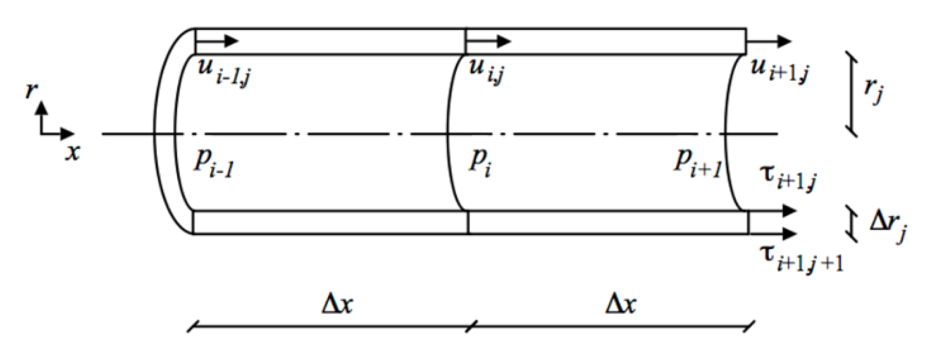
Equation (16) and, for variable mass, Equation (9), are solved on a cylindrical grid with constant step Δx in the longitudinal direction and constant area ΔA in the radial direction. Velocity is defined halfway in the radial direction, and shear stresses on the internal and external sides (Figure 1). All the calculations were carried out with 100 longitudinal steps and 50 steps in the radial mesh. Time step was .
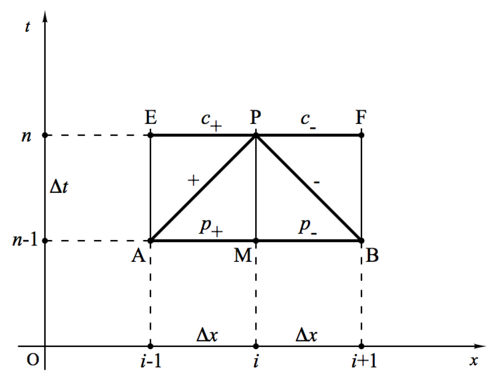
The adopted numerical scheme is defined as Z-mirror scheme, due to the shape of the characteristic line coupled with the lines along which the derivative is calculated (Figure 2). When the equation along the positive characteristic line is used, all the terms are computed on the segment AP, except the term containing the derivative with respect to of , that is computed on the segment AM in the predictor step (), and on the segment EP in the corrector step (), respectively. When the equation along the negative characteristic line is used all the terms are computed on the segment BP, except the term containing the derivative with respect to of , that is computed on the segment MB in the predictor step (), and on the segment PF () in the corrector step, respectively. Segments EP, AP and AM form a “Z”, while segments PF, BP, and MB form a “Z” as reflected in a mirror. For these reasons the scheme is defined as Z-mirror scheme and the associated model is called MOC-Z.
In the predictor step, Equation (16) is solved as
where indices , , and , refer, respectively, to directions , , and time .
In the corrector step the corresponding set of equations is
In both steps, for the evaluation of the shear stress an implicit scheme is adopted [6]. At each step, velocity components with quasi-2D models can be obtained by subtracting the negative characteristic equation from the positive one, without the need for knowing the “new” piezometric head nor the “new” auxiliary variable , as they cancel out. Then the variable is computed by adding Equations (18) and (19) (predictor step) or Equations (20) and (21) (corrector step). An analogous scheme is adopted for the 1D form of the equations.
2.7. Micro-GA
In order to compare numerical and experimental results, the calibration of and , considered as constants, has to be carried out. This was accomplished with a micro-GA. This optimization tool works with small populations, and it has the advantage, with respect to a genetic algorithm, of containing the calculation times. This is particularly useful when each evaluation of the fitness function requires the comparison of numerical results of a time-consuming mathematical model with experimental results.
The fitness of the micro-GA was evaluated as the inverse of the mean absolute error (MAE) function, as already explained by Pezzinga and Santoro [22],
where and are, respectively, the computed and measured head, and is the number of experimental values. Given that the considered duration of the experimental runs was 30 s and the experimental sampling frequency was 100 Hz, is equal to 3001. A ten-bit binary coding (giving 210 = 1024 possible values) of the parameters and , ranging, respectively, between 0 and 100 mg/m3, and between 10 and 1000 s, was used. A population size = 5 was used for the calibration of gas mass in the models with constant gass mass, where = 9 was used for the calibration of initial gas mass and relaxation time in the models with variable gas mass [22].
3. Experimental Installation
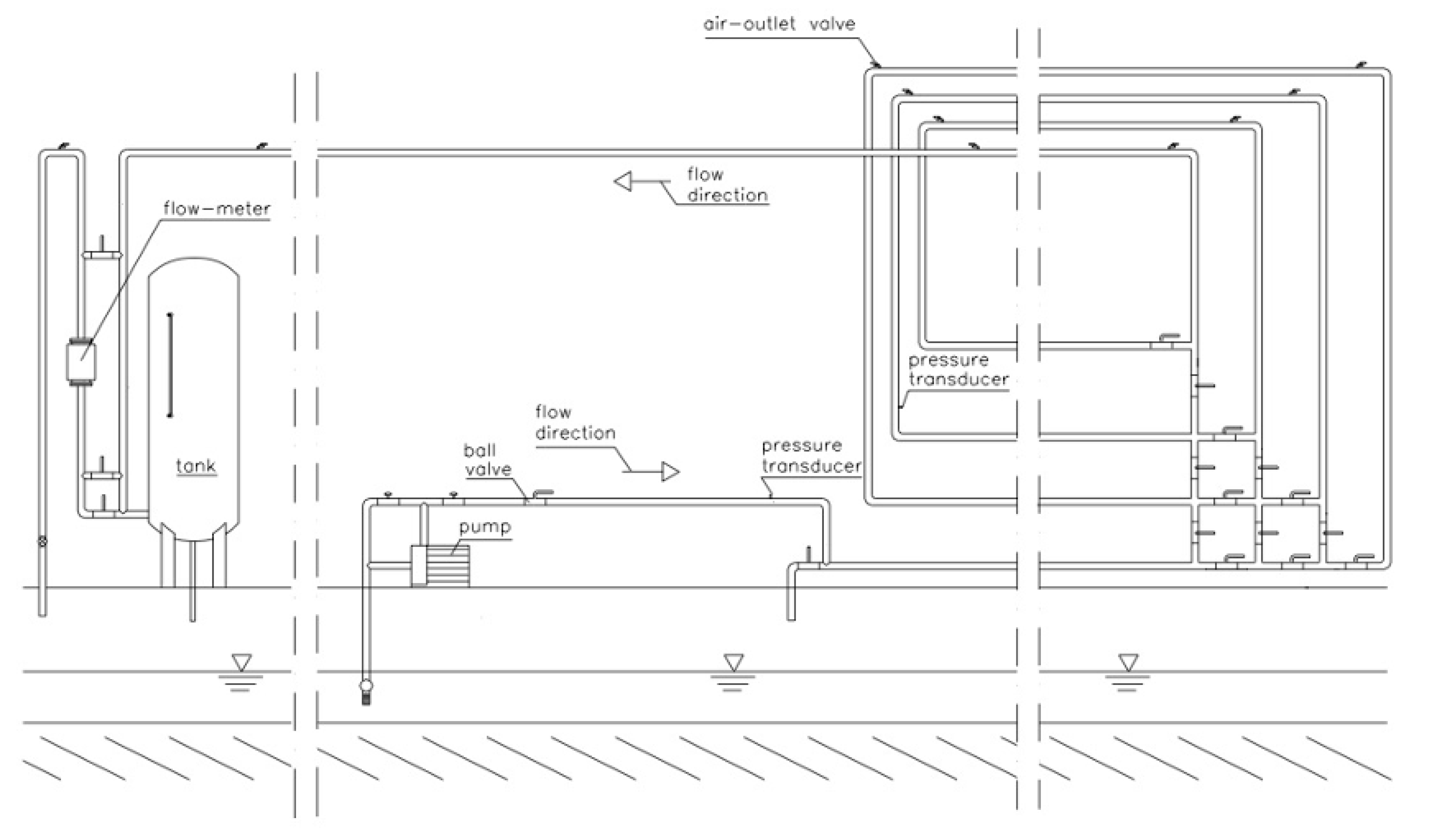
The numerical results of the proposed mathematical model were compared with experimental results of water hammer flow tests, carried out on the installation sketched in Figure 3. Such installation is composed mainly of a pipe anchored to the wall. Furthermore, previous experimental tests showed pressure traces similar to that obtained for straight pipe by Ferras et al. [8]. These considerations lead to excluding any relevant effect due to structural damping [27] or to fluid–structure interaction. The pipe is made of zinc-plated steel (internal diameter 53.9 mm, thickness 3.2 mm, modulus of elasticity 2.06 × 10¹¹ N/m2, roughness 0.1 mm, length 144.3 m) and it is fed by a centrifugal pump. A pressure tank is located at the downstream end of the pipe. The line pressure was measured with strain gauge pressure transducers, having a range of 0 to 10 bar, with maximum error of 0.5% of full-scale pressure. Discharge measurements were carried out with an electromagnetic flowmeter with adjustable full-scale velocity, with maximum errors of 0.1% of full scale. Each experimental test started from steady-state conditions by manually closing the ball valve at the upstream end of the pipe. The valve closure was estimated to take 0.04 s. Temperature as measured in all the experimental tests was 24 °C. Each physical property of water and air was indirectly evaluated as a function of the measured temperature. In Table 1, for each experimental test, values of initial discharge and static head referred to the laboratory floor are shown.
4. Analysis of Results
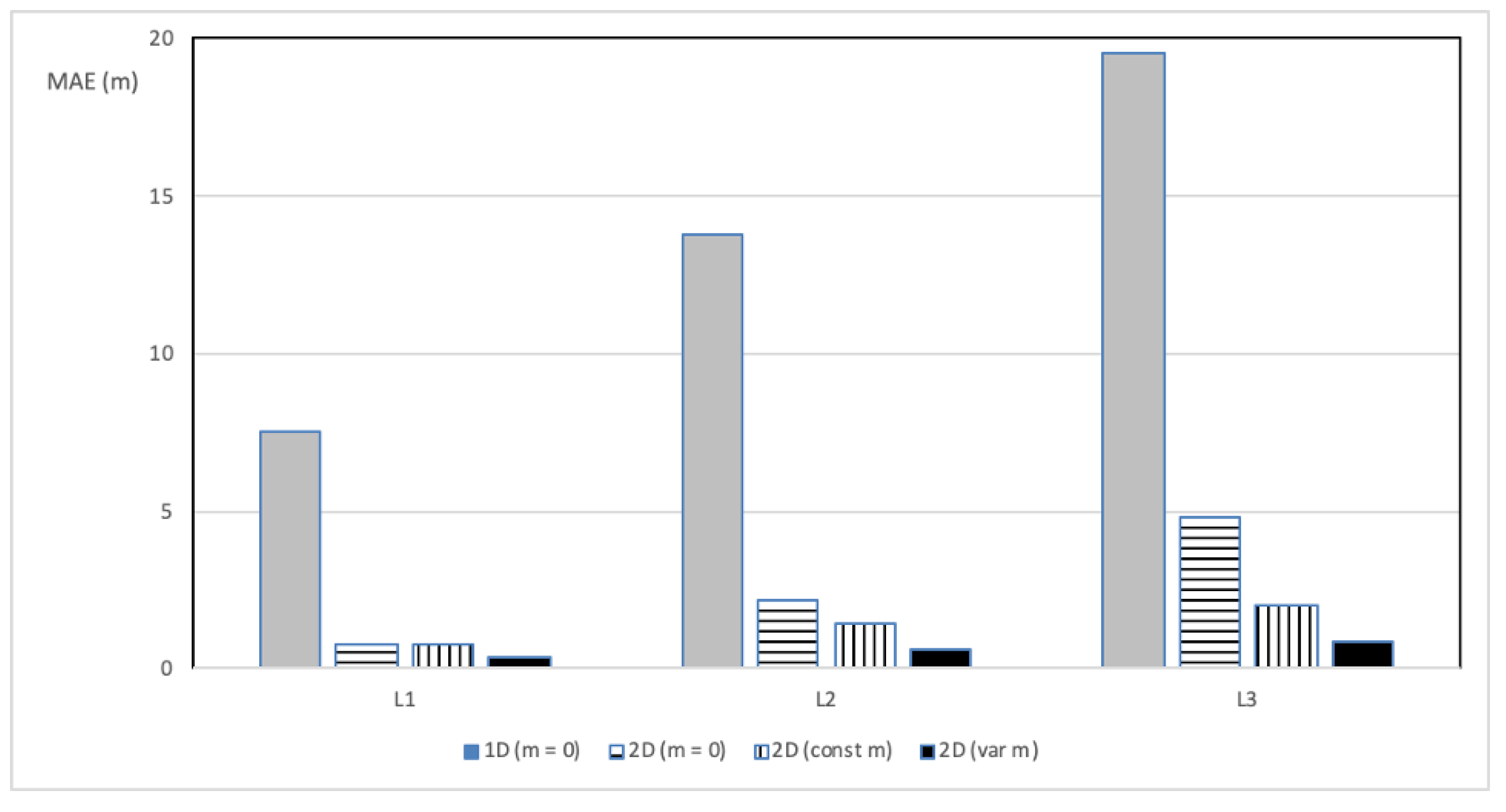
The comparison among results of all models is summarized in Figure 4, where MAEs for all tests are reported, respectively, for the 1D model without gas (1D = 0), the 2D model without gas (2D = 0), the 2D model with constant mass of gas (2D const), and the 2D model with variable mass of gas (2D var). It can be noted firstly the great decrease in MAE allowed with 2D models with respect to quasi-steady 1D models, confirming the importance of unsteady friction. Further reductions of MAE can be obtained by considering the presence of gas. When the mass of gas is considered as constant, the MAE reduction is due to the regulation of phase of the phenomenon, because the presence of gas allows the reduction of wave speed to match the experimental period and the computed one. The MAE for the models with variable mass of gas is the minimum for all the experimental tests, because the relaxation process taken into account in gas release and solution causes additional energy dissipation that allows a better reproduction of the experimental head oscillation. The ratios between the mean absolute errors of the models with and without gas release are, respectively, 47.3% for Test 1, 28.8% for Test 2, and 17.7% for Test 3.
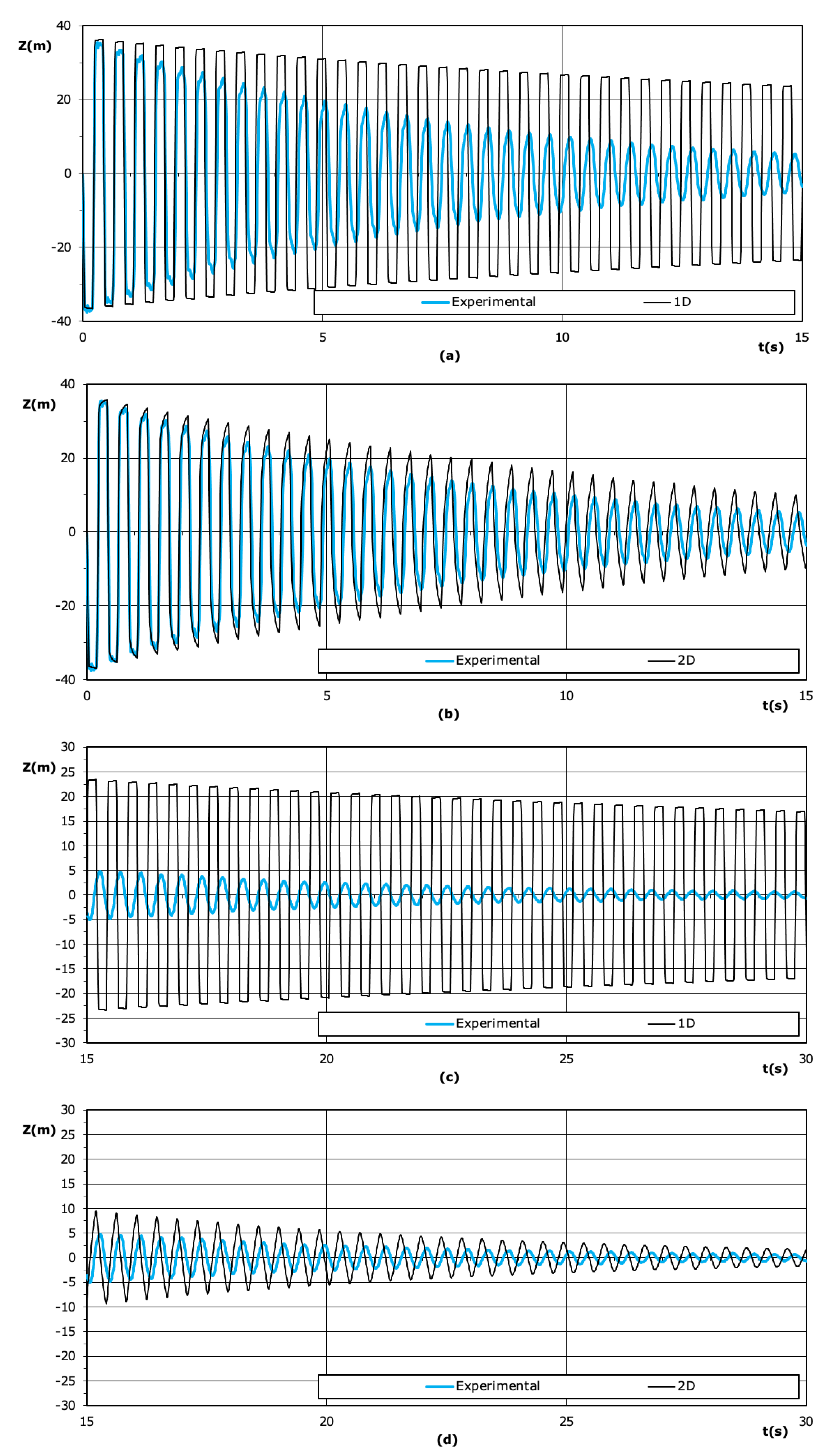
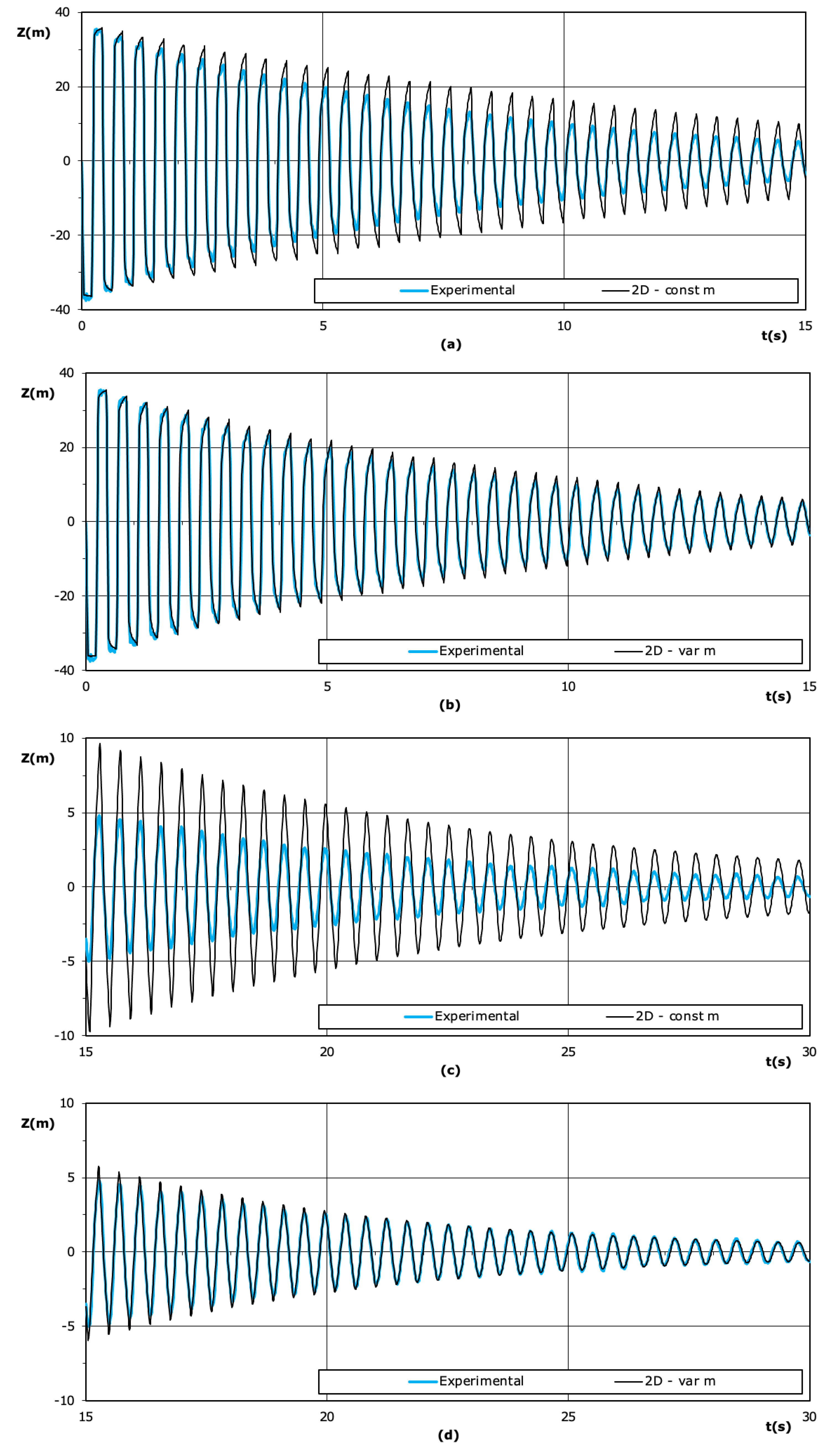
These considerations are confirmed by observing the detailed comparisons reported in Figure 5 and Figure 6 between the measured head oscillation with respect to the static head and the computed one with different models. The long duration of the test allows putting into evidence the great improvement due to the 2D flow models with respect to the 1D models (Figure 5). Furthermore, in Figure 6 the analogous results are reported for the 2D model with constant mass of gas, and with variable mass of gas. A similar behaviour to that of the model with constant mass of gas could also be obtained by reducing the wave speed of 0.5% with respect to the theoretical value (1361 instead of 1367), but with the same poor simulation of the amplitude of the oscillations. Instead, the comparison of the 2D model with variable mass of gas shows very good results in terms of phase and amplitude of the oscillations, due to cumulative effects of unsteady friction and relaxation due to gas release and solution. Longer durations were not considered due to the unreliability of smaller and smaller head oscillations.
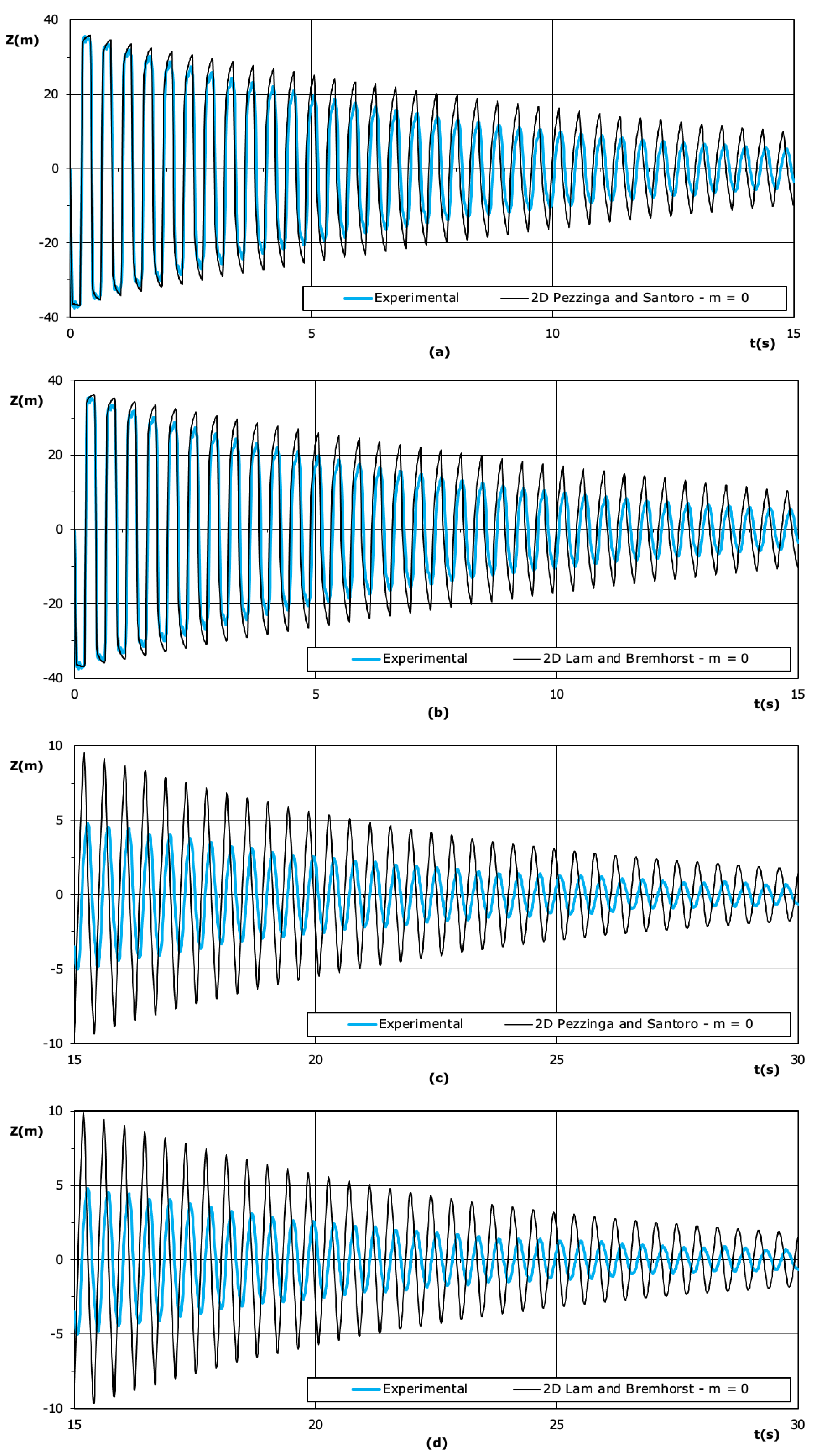
To analyse the performance of different turbulence models, Figure 7 reports the comparison of the head oscillations computed with the Santoro et al. [26] turbulence model and the Lam and Bremhorst low Reynolds number - turbulence model [23] with the experimental results. It is confirmed [7] that different turbulence models give almost the same results in terms of pressure head. Obviously more refined models can give more information on the turbulent variables, such as, for the - models, the turbulent kinetic energy and its dissipation rate .
The calibrated vales of the parameters for the 3 considered tests are reported in Table 2. An increase in the values of the mass of gas for increasing discharge already observed for transient gaseous cavitation can be noted [22]. However, this effect is probably due to particular conditions of the installation and of the experiments. With regard to the relaxation time, it can be observed that the calibrated values are of the same order of magnitude of the calibrated values for tests with transient gaseous cavitation [22].
5. Conclusions
In the present study, the use of both 1D and 2D models was considered, as well as both constant and variable gaseous mass for water hammer flow. The use of such models has the aim to examine the damping of head oscillations for tests of very long duration (about 70 periods). Main conclusions follow.
From the methodological point of view, a recently developed form of the MOC, called MOC-Z, was used, operating without the need FOR interpolation as the standard MOC for flow with liquid and gas. The calibration of the parameters was carried out with a micro-GA, to obtain results with contained computer times.
The main improvement was in the modelling of head oscillation damping results from the 2D flow schematization with respect to the 1D one with quasi-steady friction. Taking into account the mass of gas, considered as constant, reduces the MAE because it allows to phase the computed oscillations, approaching it to the observed one. If the mass of free gas is considered as a variable, taking into account a gas release and solution process, the oscillation damping is caught altogether, provided that a proper calibration of the parameters of the model is made.
In conclusion, the oscillation damping observed in water hammer flow is mainly due to unsteady friction, but other mechanisms of dissipation exist. The attribution of further energy dissipation to the gas release and solution process, here used as a hypothesis, can explain the observed oscillation damping, with values of calibrated parameters similar to other ones previously obtained. Neglected effects, in particular the thermic exchange between bubbles and surrounding liquid, could influence the values of the calibrated parameters, but, as already obtained previously [21], they do not seem capable of fully reproducing the observed pressure traces. The obtained results have some relevance in the field of water hammer research, mainly because sometimes all the energy dissipation is attributed to unsteady friction, for example calibrating the coefficients of 1D unsteady friction models using comparison of numerical and experimental pressure oscillations. The use in this study of a 2D flow model and the comparison with very long duration experimental tests allows correctly putting into evidence the role of unsteady friction and the need of other possible mechanisms of dissipation. However, the proposed hypothesized mechanism of gas release and solution has to be deepened and validated with further experimental and theoretical studies. In particular, more complex models of gas release and solution could be considered in future studies.
Funding
This research received no external funding.
Data Availability Statement
The experimental and numerical results generated or used during the study are available from the author by request.
Conflicts of Interest
The author declares no conflict of interest.
References
- Ghidaoui, M.S.; Zhao, M.; McInnis, D.A.; Axworthy, D.H. A review of water hammer theory and practice. Appl. Mech. Rev. 2005, 58, 49–76. [Google Scholar] [CrossRef]
- Pezzinga, G. Evaluation of unsteady flow resistances by quasi-2D or 1D models. J. Hydraul. Eng. 2000, 126, 778–785. [Google Scholar] [CrossRef]
- Vardy, A.E.; Hwang, K.L. A characteristics model of transient friction in pipes. J. Hydraul. Res. 1991, 29, 669–684. [Google Scholar] [CrossRef]
- Eichinger, P.; Lein, G. The Influence of Friction on Unsteady Pipe Flow. In Proceedings of the International Conference on Unsteady Flow and Fluid Transients, Durham, UK, 29 September–1 October 1992; IAHR: Durham, UK, 1992; pp. 41–50. [Google Scholar]
- Silva-Araya, W.F.; Chaudhry, M.H. Computation of energy dissipation in transient flow. J. Hydraul. Eng. 1997, 123, 108–115. [Google Scholar] [CrossRef]
- Pezzinga, G. Quasi-2D Model for Unsteady Flow in Pipe Networks. J. Hydraul. Eng. 1999, 125, 676–685. [Google Scholar] [CrossRef]
- Pezzinga, G.; Brunone, B. Turbulence, friction and energy dissipation in transient pipe flow. In Vorticity and Turbulence Effects in Fluid Structures Interactions; Brocchini, M., Trivellato, F., Eds.; WIT Press: Southampton, UK, 2006; pp. 213–236. [Google Scholar]
- Vardy, A.E. On Sources of Damping in Water-Hammer. Water 2023, 15, 385. [Google Scholar] [CrossRef]
- Ferras, D.; Manso, P.A.; Schleiss, A.J.; Covas, D.I. Experimental distinction of damping mechanisms during hydraulic transients in pipe flow. J. Fluids Struct. 2016, 66, 424–446. [Google Scholar] [CrossRef]
- Kranenburg, C. Gas release during transient cavitation in pipes. J. Hydraul. Div. 1974, 100, 1383–1398. [Google Scholar] [CrossRef]
- Wiggert, D.C.; Sundquist, M.J. The Effect of Gaseous Cavitation on Fluid Transients. J. Fluids Eng. 1979, 101, 79–86. [Google Scholar] [CrossRef]
- Wylie, E.B. Low void fraction two-component two-phase flow. In Unsteady Flow and Fluid Transients; Bettess, R., Watts, J., Eds.; Balkema: Rotterdam, The Netherlands, 1992; pp. 3–9. [Google Scholar]
- Huygens, M.; Verhoeven, R.; Van Pocke, L. Air entrainment in water hammer phenomena. WIT Trans. Eng. Sci. 1998, 18, 10. [Google Scholar]
- Hadj-Taieb, E.; Lili, T. Transient flow of homogeneous gas-liquid mixtures in pipelines. Int. J. Numer. Methods Heat Fluid Flow 1998, 8, 350–368. [Google Scholar] [CrossRef]
- Lee, T.S.; Low, H.T.; Nguyen, D.T. Effects of air entrainment on fluid transients in pumping systems. J. Appl. Fluid Mech. 2007, 1, 55–61. [Google Scholar]
- Lee, T.S.; Low, H.T.; Huang, W.D. Numerical study of fluid transient in pipes with air entrainment. Int. J. Comput. Fluid Dyn. 2004, 18, 381–391. [Google Scholar] [CrossRef]
- Bergant, A.; Simpson, A.R.; Tijsseling, A.S. Water hammer with column separation: A historical review. J. Fluids Struct. 2006, 22, 135–171. [Google Scholar] [CrossRef]
- Fanelli, M. Hydraulic Transients with Water Column Separation; IAHR Working Group 1971–1991 Synthesis Report; IAHR: Delft, The Netherlands; ENEL-CRIS: Milan, Italy, 2000. [Google Scholar]
- Landau, L.D.; Lifshitz, E.M. Fluid Mechanics: Course of Theoretical Physics; Pergamon Press: London, UK, 1959; Volume 6. [Google Scholar]
- Pezzinga, G. Second viscosity in transient cavitating pipe flows. J. Hydraul. Res. 2003, 41, 656–665. [Google Scholar] [CrossRef]
- Cannizzaro, D.; Pezzinga, G. Energy dissipation in transient gaseous cavitation. J. Hydraul. Eng. 2005, 131, 724–732. [Google Scholar] [CrossRef]
- Pezzinga, G.; Santoro, V.C. MOC-Z Models for Transient Gaseous Cavitation in Pipe Flow. J. Hydraul. Eng. 2020, 146, 04020076. [Google Scholar] [CrossRef]
- Lam, C.K.G.; Bremhorst, K.A. Modified Form of the k-ε Model for Predicting Wall Turbulence. J. Fluids Eng. 1981, 103, 456–460. [Google Scholar] [CrossRef]
- Wylie, E.B.; Streeter, V.L. Fluid Transients in Systems; Prentice-Hall: Englewood Cliffs, NJ, USA, 1993. [Google Scholar]
- Zielke, W.; Perko, H.D.; Keller, A. Gas Release in Transient Pipe Flow. In Pressure Surges, Proceedings of the 6th International Conference, Cambridge, UK, 4–6 October 1989; BHRA: Cranfield, UK, 1990; pp. 3–13. [Google Scholar]
- Santoro, V.C.; Crimì, A.; Pezzinga, G. Developments and limits of discrete vapor cavity models of transient cavitating pipe flow: 1D and 2D flow numerical analysis. J. Hydraul. Eng. 2018, 144, 04018047. [Google Scholar] [CrossRef]
- Budny, D.D.; Wiggert, D.C.; Hatfield, F.J. The influence of structural damping on internal pressure during a transient pipe flow. J. Fluids Eng. 1991, 113, 424–429. [Google Scholar] [CrossRef]
Figure 1.
Grid for the 2D models.

Figure 2.
Lines for numerical resolution with the Z-mirror scheme.

Figure 3.
Experimental installation.

Figure 4.
Mean absolute errors of different models with respect to experimental data.

Figure 5.
Comparison of head oscillations computed with the 1D or 2D model without free gas with the experimental results for Test L3: (a) 1D model, = 0 − 15 s; (b) 2D model, = 0 − 15 s; (c) 1D model, = 15 − 30 s; (d) 2D model, = 15 − 30 s.
Figure 5.
Comparison of head oscillations computed with the 1D or 2D model without free gas with the experimental results for Test L3: (a) 1D model, = 0 − 15 s; (b) 2D model, = 0 − 15 s; (c) 1D model, = 15 − 30 s; (d) 2D model, = 15 − 30 s.

Figure 6.
Comparison of head oscillations computed with the 2D model with constant or variable mass of free gas with the experimental results for Test L3: (a) 2D model with constant mass of free gas, = 0 − 15 s; (b) 2D model with variable mass of free gas, = 0 − 15 s; (c) 2D model with constant mass of free gas, = 15 − 30 s; (d) 2D model with variable mass of free gas, = 15 − 30 s.

Figure 7.
Comparison of head oscillations computed with the 2D present model or with the Lam and Bremhorst [23] model without free gas with the experimental results for Test L3: (a) 2D present model, = 0 − 15 s; (b) 2D Lam and Bremhorst model, = 0 − 15 s; (c) 2D present model, = 15 − 30 s; (d) 2D Lam and Bremhorst model, = 15 − 30 s.


Table 1.
Physical parameters of the experimental tests.
| Test | (L/s) | (m/s) | (m) | |
|---|---|---|---|---|
| L1 | 0.207 | 0.091 | 68.12 | 5300 |
| L2 | 0.409 | 0.179 | 66.87 | 10,500 |
| L3 | 0.598 | 0.262 | 60.08 | 15,400 |
Table 2.
Values of calibrated parameters.
| Test | 2D—Constant Mass | 2D—Variable Mass | |
|---|---|---|---|
| (mg/m3) | (mg/m3) | (s) | |
| L1 | 1.96 | 0.00 | 753.2 |
| L2 | 17.30 | 6.16 | 754.2 |
| L3 | 28.64 | 14.96 | 815.2 |
Disclaimer/Publisher’s Note: The statements, opinions and data contained in all publications are solely those of the individual author(s) and contributor(s) and not of MDPI and/or the editor(s). MDPI and/or the editor(s) disclaim responsibility for any injury to people or property resulting from any ideas, methods, instructions or products referred to in the content. |
© 2023 by the author. Licensee MDPI, Basel, Switzerland. This article is an open access article distributed under the terms and conditions of the Creative Commons Attribution (CC BY) license (https://creativecommons.org/licenses/by/4.0/).
Share and Cite
MDPI and ACS Style
Pezzinga, G. Gas Release and Solution as Possible Mechanism of Oscillation Damping in Water Hammer Flow. Water 2023, 15, 1942. https://doi.org/10.3390/w15101942
AMA Style
Pezzinga G. Gas Release and Solution as Possible Mechanism of Oscillation Damping in Water Hammer Flow. Water. 2023; 15(10):1942. https://doi.org/10.3390/w15101942
Chicago/Turabian StylePezzinga, Giuseppe. 2023. "Gas Release and Solution as Possible Mechanism of Oscillation Damping in Water Hammer Flow" Water 15, no. 10: 1942. https://doi.org/10.3390/w15101942
Note that from the first issue of 2016, this journal uses article numbers instead of page numbers. See further details here.