1. Introduction
Floods are described as a major type of natural disaster that occur worldwide, and they have become one of the most serious environmental issues [
1]. According to Tehrany et al. [
2] and Foody et al. [
3], floods cause massive infrastructure damage and loss of life worldwide. Floods have also caused severe environmental disasters in most arid and semiarid regions [
4]. Saudi Arabia, for example, is one of the countries that suffers from the negative effects of floods in some of its regions, such as Riyadh, Najran [
5,
6], and many others.
According to Elkhrachy [
6], about 16% of the population of Najran city has been affected by floods. Flooding is also a serious problem for the Riyadh region and threatens the environment, human life, infrastructure, and economic development, especially in the northern and northeastern parts of the region [
5]. An intense rainstorm (23.7 mm) on 19 November 2013 in Riyadh caused widespread flooding in many parts of the region. According to the Al-Riyadh Newspaper, this flood affected the infrastructure, such as roads and parking lots in many cities including Riyadh, and resulted in severe damage for residential properties, as shown in the photos presented in
Section 2. All these losses could have been avoided or minimized if an adequate flood vulnerability map was provided, and the conditions for flood occurrence were well defined. Accordingly, an approach that enables the accurate identification of the areas most prone to flooding and optimum factors leading to flood susceptibility is required to implement effective mitigation programs that reduce or prevent future increases in flood incidence.
The Wadi Hanifah drainage area has undergone an extensive land use change due to rapid population increase and urban development since 1972, which has negatively affected agricultural lands [
7,
8,
9]. As a result, around 70% of the Riyadh province is located inside the Wadi Hanifah’s drainage basin and has become susceptible to flood hazards [
9].
A strategic development plan was proposed for the Wadi by the high commission for the development of Riyadh (ADA) in 1994 and was officially finished in 2003 [
10], and it had five phases. The main aim of this plan was to maximize the benefit from Wadi Hanifah’s catchment. This development plan has been updated into the Riyadh Metropolitan Structural Plan 2030, which includes broad goals for urban infrastructure and land use, while at the same time setting out a basis for city development policies and procedures, such as important development areas, and the intention to use public lands and habitable, industrial, and protected areas [
11]. Therefore, the results of the current study will present suggestions for the areas that will be included in the land use development as it highlights the areas that are highly prone to flooding in the future.
One of ways to identify the most prone areas to flooding is forecasting, which can be used as a tool to reduce flood-related damages and economic losses [
12]. Moreover, mapping the spatial distribution of flood-prone areas is also a good tool that can be used to mitigate or avoid the effects of future flood events [
13]. In light of these solutions, many studies in recent years have focused on mapping and identifying flood susceptibility areas (with the help of remote sensing data and GIS capabilities) using variety of complex techniques, including machine learning methods [
9,
10,
11,
12,
13,
14,
15,
16,
17,
18], analytical hierarchy process (AHP) [
8,
13,
14,
15,
16,
17,
19,
20,
21,
22], and frequency ration (FR) [
1,
2,
18,
23]. However, the contributing factors to flooding were inconsistent among all these studies in terms of number and significance. For example, many hydrological, topographical, and ecological parameters are widely recognized as significant and non-important factors that influence the occurrence of floods. Previously, Kazakis et al. [
22] introduced a new flood hazard index (FHI) to map and assess flood hazard areas in the Rhodope–Evros region in northern Greece using seven parameters, including: flow accumulation, distance from drainage network, elevation, land use, rainfall intensity, and geology. They revealed that geology was the least contributing parameter for flood occurrence in the study area. In contrast, three parameters, including the elevation, the distance to the drainage network, and the slope, were the most contributing parameters to the occurrence of floods. Recently, Msabi and Makonyo [
19] found that elevation, slope, geology, Dd, flow accumulation, land use/land cover, and soil type were effective variables to map flood susceptibility areas in the Dodoma region, and they found that among these seven parameters, only slope, elevation, and Dd had greater influence on the flood occurrence in the Dodoma region. In addition, Kourgilas and Karatas [
24] conducted a study in Greece to estimate the spatial distribution of hazardous areas based only on six factors: flow accumulation, slope, land use, precipitation intensity, geology, and elevation; their results indicated that the six parameters perform better for predicting potential flood susceptibility areas.
Additionally, several authors have reported that an effective flood can occur in areas characterized by concave and flat slopes [
1,
25]. For example, Termeh et al. [
1] found that plan curvature with flat and concave slopes have the largest contributions to the occurrence of floods. According to their results, this factor has the largest frequency ration, 95%, compared to the most effective factors, i.e., slope, rainfall, and altitude, and they stated that lithology was the least important factor for the flood occurrence. In contrast to these views, other researchers have reported that profile curvature contributes less regarding flooding. For example, Khosravi et al. [
26], in a comparative analysis, rejected the direct links between profile curvature and flood occurrence. The elevation, slope, and TWI factors, for instance, were recognized as the most contributing factors to the occurrence of floods [
2,
12,
18,
27,
28]. On the other hand, other results obtained by Wang et al. [
18], using the random forest statistical technique, showed that slope, NDVI, SPI, soil texture, distance to the drainage network, and land use pattern were the least contributing factors with respect to mapping flood incidence in the Dongjiung River Basin in China. The runoff (Q) factor, in turn, has been found to be less significant in the occurrence of flooding in different areas. Tehrany et al. [
2], based on a Cohen’s Kappa index, have declared that runoff (Q) was the least contributing factor to the occurrence of flooding in their area of study, and they concluded that reliable results can be obtained by removing the runoff (Q) factor from the computation of final flood susceptibility index (FSI). In contrast to this result, runoff (Q) was recognized as an effective driving factor for the occurrence of flooding in the Dongjiung River Basin in China [
18] and in Najran city in Saudi Arabia [
6]. In addition, unlike other studies, basin characteristics, such as geomorphometry, land use/land cover type, size, and location of rainstorm, are also considered effective variables that control the flood peak in arid and semiarid regions [
4]. Das [
12], using analytical hierarchy process (AHP), showed that Dd had major impacts on flood occurrence in the Ulhas catchment. An increase in the probability of flooding with urbanization has also been reported by some authors [
16,
21]. Hence, human activities, such as rapid urbanization and logging [
2,
27], and climate change, such as extreme precipitation events [
5], can increase the likelihood of flooding.
The spatial multicriteria decision analysis methods are proficient for enhancing the clearness and diagnostic precision of land use decisions [
29,
30]. Applied works in MCDA methods have become more prevalent in studies related to land appropriateness [
31]. The innovative MCDA approaches comprising Electre, Maut, Promethee, and fuzzy set theory, in addition to random set theory, offer extra modern procedures to study ambiguous or imprecise data [
32]. The theory of fuzzy set methods is considered the most public approach that deals with inaccurate and ambiguous problems [
29]. However, most of the empirical studies have applied fuzzy methods without a proportional investigation to examine whether applying extra modernized methods such as fuzzy AHP will cause a substantial change compared to normal AHP. Furthermore, choosing further advanced methods such as fuzzy AHP, which can merely be observed as a black box by stakeholders, does not produce dissimilar results. However, in additional comprehensive planning, recognizing spatial limits is essential (for example, forming a master plan). In that context, the primary reason for the popularity of the AHP is that it is very convenient to implement within the environment of GIS by means of map algebra processes and cartographic modeling. The approach is also easy to understand and instinctively tempting to decision makers.
The analytical hierarchy process (AHP) and weighted product model (WPM) are prevalent techniques based on the collective weighting model [
33]. They have been used in two common means within the environment of GIS. Firstly, they could be used to develop the weights related to map layer characteristics, merging weights with the layers of the attribute map in a way comparable to the weighted improver grouping means. This method is significant for issues concerning a big number of substitutes, when it is difficult to achieve a pairwise comparison of the substitutes. Secondly, their values could be utilized in order to combine primacy for the entire the hierarchy structure level comprising the level signifying substitutes so that a comparatively trivial number of substitutes could be assessed [
34].
Advantageously, AHP is a proficient technique that could be employed to distribute numerous parameters into a cluster of pairwise evaluations followed by incorporating the outcome [
35,
36]. Decision makers with different specializations have confirmed that the integration of GIS with AHP in the MCDA context is operative in numerous studies associated with the assessment of natural hazards such as floods. On the other hand, the AHP technique has been capable in achieving plentiful environmental and climatic applications, for instance, mapping soil erosion threats [
37], landslide susceptibility mapping, and zoning potential groundwater [
38]. The efficiency of a such technique (i.e., integration of GIS with AHP in MCDA context) in mapping hazards is primarily due its capability to handle data shortage issues [
39]. Nevertheless, there have been some caveats in AHP as one of the MCDA-applied techniques, as GIS employments of the weighted synopsis processes are frequently applied without complete understanding of the assumptions underlying the technique. Furthermore, the technique is mostly achieved regardless of whether there is complete awareness of the senses of the dual serious features of the weighted summation model; the weights assigned to attribute maps as well as the measures of the originating commensurate attribute maps. Malczewski [
40] presented debates on some characteristics of the improper usage of the technique.
Numerous studies other than AHP and WPM have been applied for flood risk assessment, such as numerical models [
41,
42], which have been widespread approaches for flood risk studies. Hydrological and hydrodynamic models have been largely utilized for assessing floods with respect to size, scope, and occurrence [
41,
43]. Hydrological models, for example, the Normal Distribution or P-III Distribution models, deal mostly with line-type flood spreading. The runoff yield model, an additional hydraulic model, principally examines the flood channeling problems of water courses. Such numerical models are able to process many data and reproduce important info about flood danger. However, the most mutual and challenging matter in such approaches is the rareness or absence of hydrometeorological data [
40].
The first attempt to map flood susceptibility zones over the Riyadh region was conducted by Mahmoud and Gan [
5]. They used ten parameters to map flood susceptibility and assess its risk by employing an AHP model for parameter weighting. Their study concluded that the occurrence of floods in the Riyadh region was triggered by two factors, namely, runoff (Q) and flow accumulation.
Although the previous study conducted in the study area provided reliable results regarding flood susceptibility mapping and assessment, the variables contributing to the occurrence of floods need further investigation [
5]. Despite the fact that the ability to determine the sites most susceptible to flooding is well documented, as shown in the above literature, the links between flood occurrence and its parameters are not easy to determine. Therefore, this study aimed to (1) map and assess flood susceptibility zones in the Wadi Hanifah drainage basin using the AHP and WMP models and (2) identify the key/optimum variables leading to flood susceptibility using a correlation matrix and OIF. Our primary hypothesis was that the variable with the largest mean, least variance (CV%), and least correlation would be the most influential variable contributing to flooding in the study area. A complementary objective was to compare the performance of the AHP and WPM models regarding the accuracy of flood susceptibility mapping. The outcome of this study will assist local authorities (e.g., Civil Defense Authority), engineers, and decision makers in dealing with the risks related to floods and also help develop a strategic plan for urban development, and can be used as a support to protect against flood risks in the future.
2. Materials and Methods
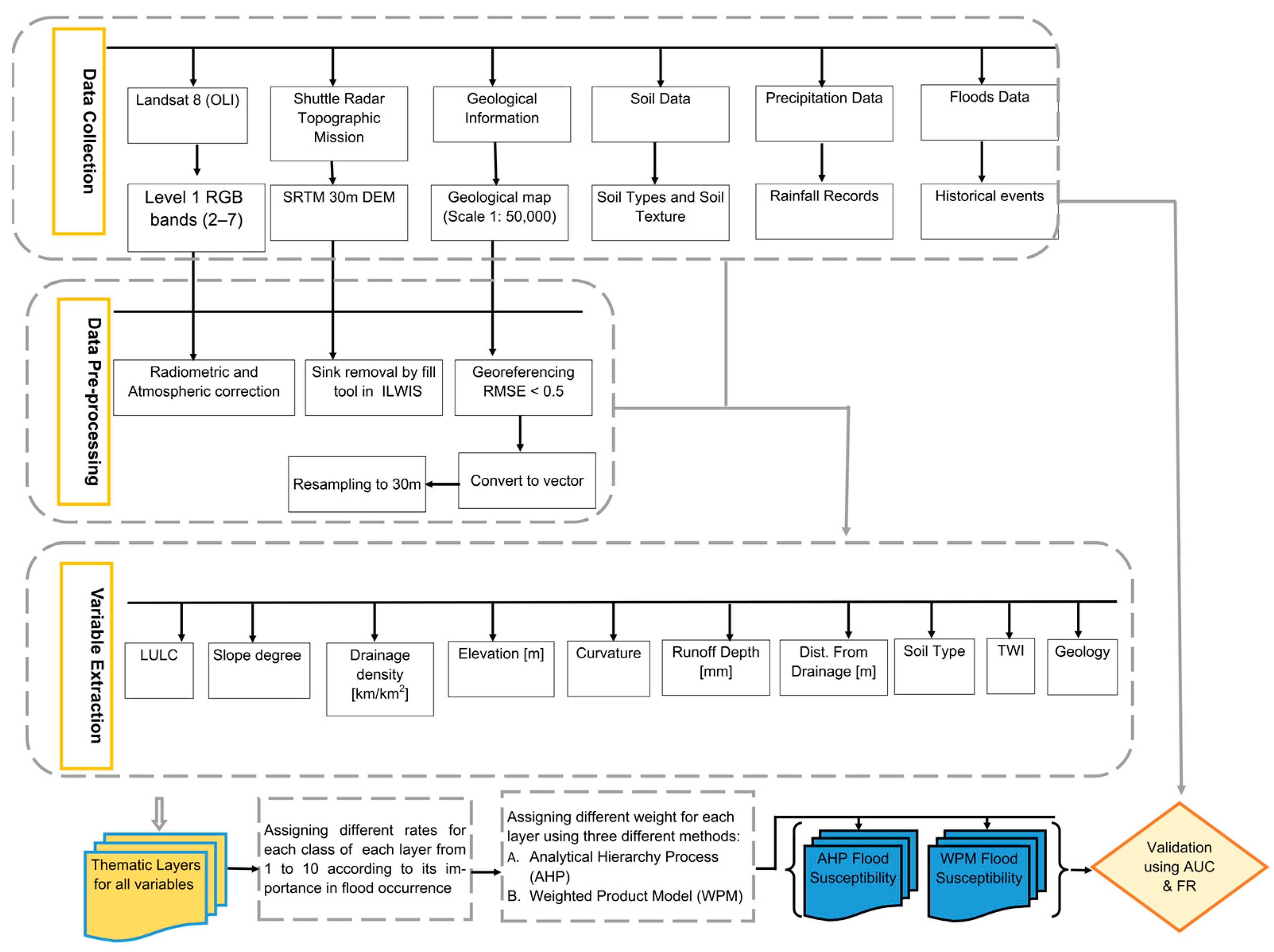
The workflow for achieving this study entails four main procedures: first, mapping the effective variables in the occurrence of floods using the data shown in
Table 1; second, the analysis and modeling of flood susceptibility; third, the validation of flood susceptibility maps; and finally, the assessment of variables’ importance in flood susceptibility (
Figure 1). These steps require separate methodologies, which are provided in the following subsections.
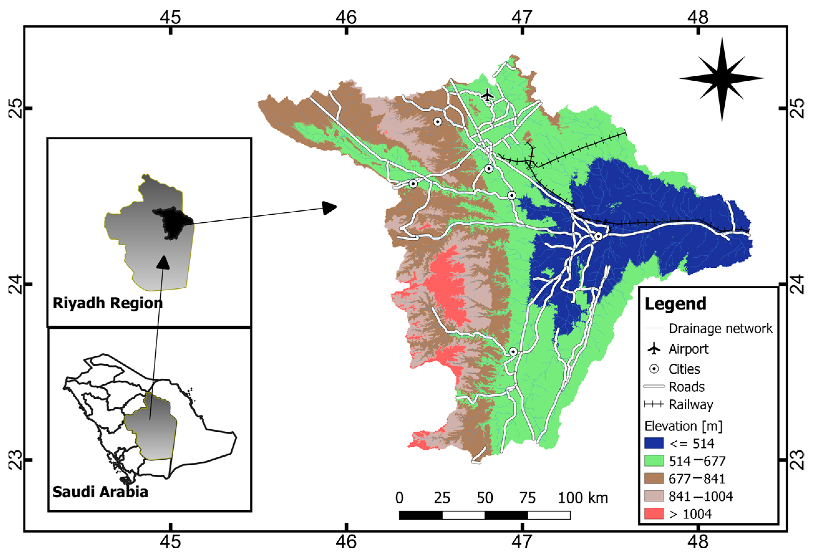
The Wadi Hanifah drainage basin (32,897.24 km
2), one of the major natural habitats of algae and various aquatic plants [
44], is located in the Riyadh region, between latitudes 23°04′ N–25°10′ N and longitudes 45°23′ E–48°15′ E (
Figure 2). Wadi Hanifah is one of the main drainage systems in the region, and comprises two main branches, Wadi Aysan and Batha, and collects flood water from these tributaries. The area is characterized by western mountainous land (e.g., Tuwaig mountain), low elevations in the northern and eastern parts of the basin, and gentle slopes in the central and eastern parts of the basin. Its elevation ranges between 368 and 1175 m above mean sea level. It is circulated with a main W-E orientation. Its length and width are about 150 km and 30 km, respectively [
8]. Moreover, in one year, about 200,000 cubic meters of water is discharged into it. To increase the groundwater recharge, around seven dams have been established on the Wadi [
45]. Most of the residential areas are situated at low altitudes, which makes them more prone to flooding. The main cities are Riyadh, which has a population of 7.677 million according to the 2018 census, and an area of 1973 km
2, and Al-Kharj, which has a population of 376 thousand.
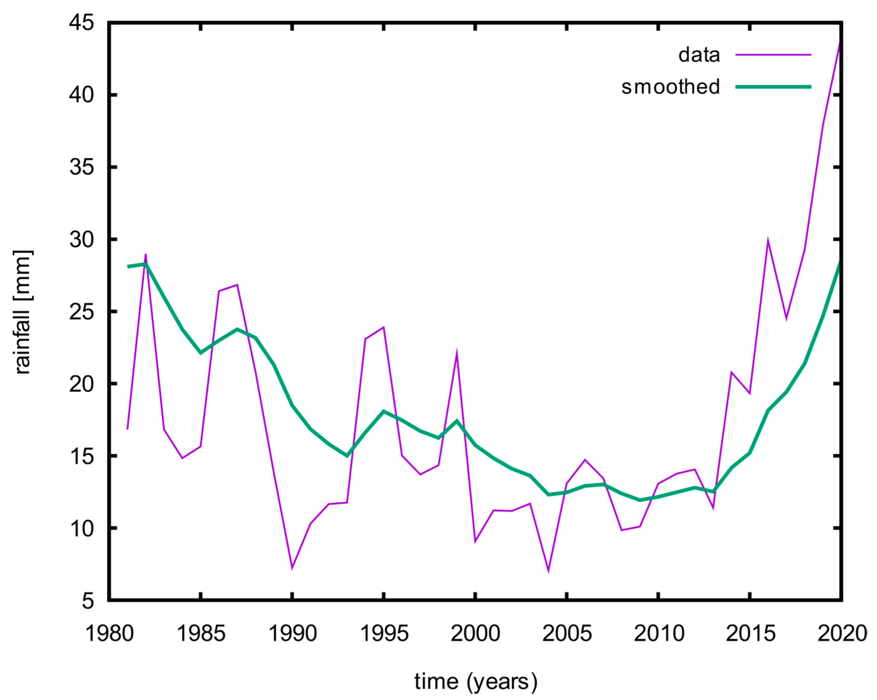
The Wadi Hanifah basin has a dry climate with an average annual temperature of over 45 °C during the summer (June to August). During the winter (January and February), the temperature varies between 2 and 25 °C. The annual precipitation is about 84.4 mm with a large interannual variance, as shown in the precipitation variance in
Figure 3. Most of the basin area (32.17%) is made of two types of geological formations: (a) Jurassic formations, primarily in the western part of the study area, and (b) Cretaceous formations, which primarily exist in the eastern part of the study area.
The area covered by the Wadi Hanifah drainage basin has suffered from the effects of natural disasters, such as flooding [
9,
46]. For example, large flood events have occurred in the Riyadh province and led to serious damage to the traffic and infrastructure [
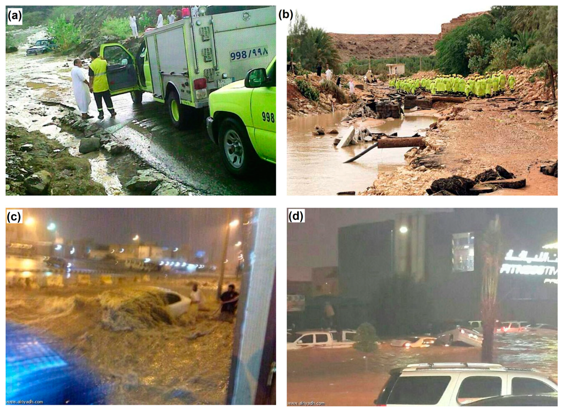
46]. Moreover, during the past ten years, one of the most important events which occurred within the basin was the flood on 19 November 2013, which caused a severe damage to the residential properties and infrastructure of Riyadh city and some of its neighborhoods (
Figure 4); therefore, this basin was considered a suitable case study area, and the identification of flood-prone areas and the variables underlying them became the main objective of this study.
2.1. Data Acquisition and Variables Extraction
Several types of data (
Table 1) were used to extract (10) variables for flood susceptibility mapping. The geological and soil maps were downloaded freely from the US Geological Survey (USGS) World Oil and Gas Resource Assessment website (
https://certmapper.cr.usgs.gov/ (accessed on 5 December 2022)) and Food and Agriculture Organization of the United Nations (FAO) (
https://www.fao.org/soils-portal/data-hub/ (accessed on 5 December 2022)), respectively. The SRTM-DEM and Landsat-8, an Operational Land Imager and Thermal Infrared Sensor (OLI and TIRS), satellite products were freely obtained from the US Geological Survey (USGS) Earth Explorer website (
http://earthexploere.usgs.gove/ (accessed on 5 December 2022)). We obtained the daily rainfall for the date 19 November 2013 from the Riyadh meteorological station report, Saudi Arabia (
https://ncm.gov.sa/ (accessed on 5 February 2022)). These data were preprocessed by employing the capability of different open source software, including R i386 4.1.2, QGIS 3.18, and ILWIS 3.4 GIS software programs.
On the other hand, the historical flood events data were collected from local sources (newspapers and reports), including Al Riyadh (Arabic;
https://www.alriyadh.com/ (accessed on 5 February 2022)), Al Jazirah (Arabic;
https://www.al-jazirah.com/ (accessed on 5 February 2022)), and Al Eqtisadiah newspapers (
https://www.aleqt.com/ (accessed on 5 February 2022)), as described previously [
20]. All these three sources were reviewed for news related to flood events that occurred previously in the study area from 2010 to 2015. This period was selected due to the noticed frequency of flood occurrence in the specified time span, according to reports provided by local residents in the study area. About 23 locations were identified and tabulated using an excel sheet, so that the data entailed the location names, the date, the month, and the year of the individual event. Google Earth Pro version 2018 was then used to extract the (x and y) of each location, and then the tabulated data were vectorized, making use of the conversion tools of the ILWIS 3.4 GIS software. Then, the transform point map tool of ILWIS 3.4 was used to transform the coordinates of these points from “LaLoWGS 1984” in degrees to a projected coordinate system “WGS 1984 UTM zone 38N” to match the other data set. The data types, sources, and uses are briefly described in
Table 1.
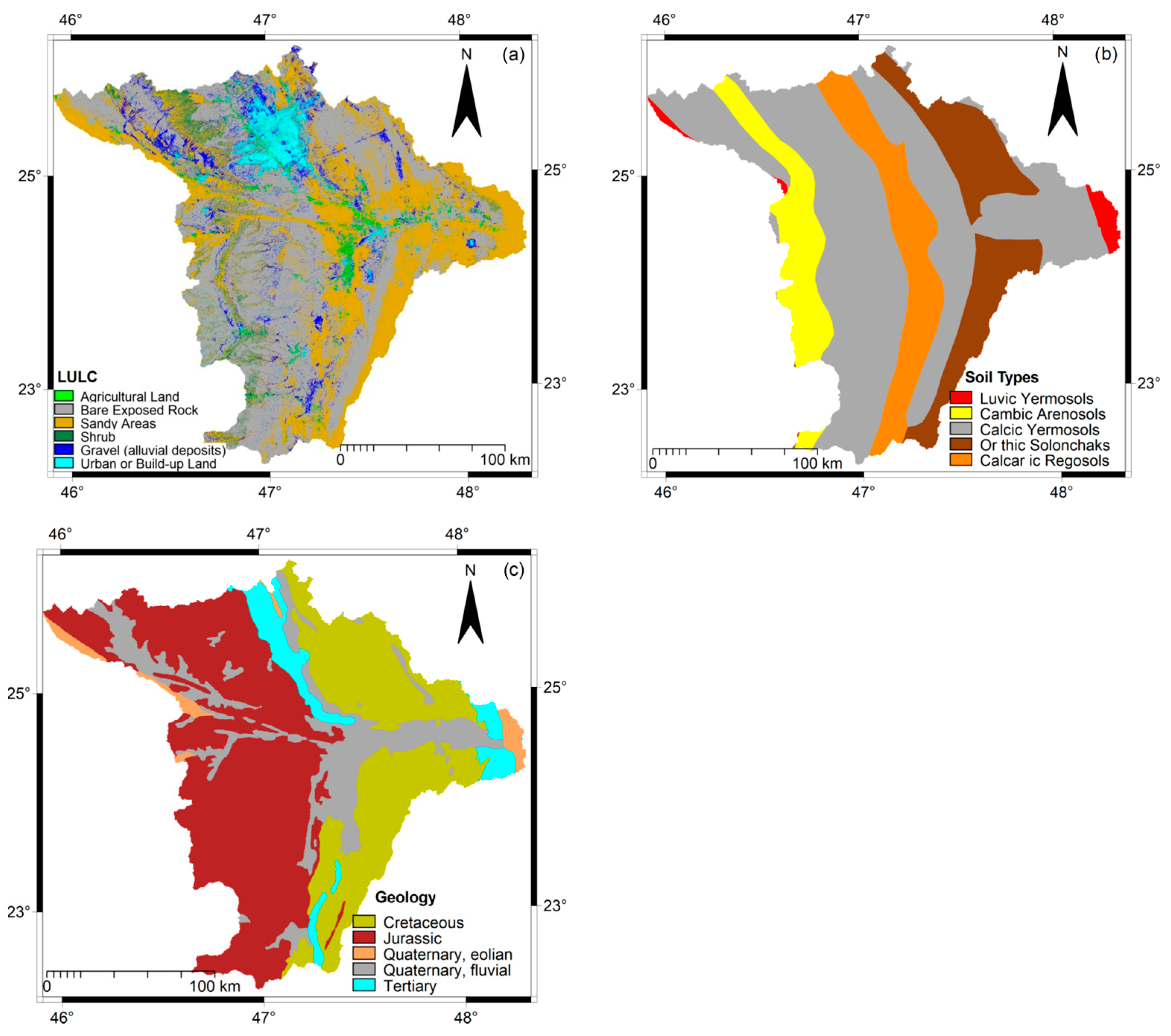
The selected most effective factors that were assumed to have a great influence on flooding are, namely, land use/cover, distance from existing river or drainage network, Dd, elevation, slope, curvature, soil type, topographic wetness index (TWI), runoff (Q), and geology or lithology. Most of the studies related to modeling and mapping flood susceptibility, specifically studies conducted in arid and semiarid areas, selected these variables as the most effective factors [
15,
17,
28]. In this study, all these factors were categorized into three groups of variables: (1) topographical variables, including elevation, slope, and curvature; (2) hydrological variables, including runoff (Q), Dd, TWI, and distance from drainage network; and (3) environmental variables, including land use/land cover, geology, and soil type. The detailed procedures used to extract every parameter are described in the subsections below.
2.1.1. Environmental Variables Extraction
The land use/cover type directly impacts the frequency of flood occurrence by increasing or decreasing runoff (Q) volume and infiltration rate [
47], as runoff (Q) increases in urban areas and decreases in vegetated areas [
15]. In the present study, the land use/cover map (see
Figure 5a) was constructed from Landsat-8 OLI image data (path/raw: 165/43; acquired on 3 March 2020;
Table 1) by applying k-Nearest Neighbor (k-NN) machine learning classifier [
48] using R software (version 4.1.2), where a Cart package was used [
49]. The final values used for the K-NN model were kmax = 9, distance = 2, and kernel = optimal. Training samples were collected from Google Earth Pro high-resolution satellite images using a visual interpretation technique. In total, around 1006 samples (region of interest (ROI)) were collected to represent each of the land use/cover categories. Six separate land use/cover types were identified based on Anderson’s classification Level 1 scheme [
50], including: agricultural land, bare exposed rock, sandy areas, shrub land, grave (alluvial deposit), and build-up area, as shown in
Figure 5a. Cross validation (5-fold, repeated 5 times) was used as an accuracy assessment method. The overall classification accuracy was 0.903 with a kappa coefficient equal to 0.874, which is quite acceptable for the purpose of this study.
The Landsat-8 sensor produces data in 11 spectral bands at spatial resolutions ranging from 15 to 100 m. Bands 2–6 were selected for the purpose of this study as they provided the most appropriate spatial resolution, which is 30 m. Prior to the classification and to obtain high-quality products, the images were carefully preprocessed using the standard techniques [
51,
52,
53], aiming to minimize the image noise, atmospheric effect, and variation between the spectral bands, and to maximize the image spectral information used for image classification and analysis. The preprocessing included atmospheric and radiometric corrections of the remotely sensed data, using the Semi-Automatic Classification Plugin (SCP) [
54,
55], which is available in the QGIS open source software. The gain and offset coefficients available in the satellite image metadata file were used to convert the image bands into radiance and from radiance to top-of-atmospheric (TOA) reflectance. The atmospheric correction was achieved by SCP’s dark object subtraction technique [
56]. A sub-scene covering the study site was selected and converted into the R program for the purpose of land use/land cover classification. The classification output was directly imported into the ILWIS 3.4 GIS program, and the obtained land use/land cover map’s classes were then assigned rates ranging from 1 (minimum impact to flood susceptibility) to 10 (maximum impact to flood susceptibility) according to their permeability. The urban or build-up areas had the highest rates in comparison to agricultural or shrub land.
Soil type and texture are effective variables in the occurrence of floods because they determine the water holding capacity and infiltration capacity of an area [
57]. Some types of soil, for example, clay soil, can cause more flooding than other types [
11]. The “soil type” data used in this study were provided by the Food and Agriculture Organization (FAO) [
58] in a raster format. The texture of the various soil types in the study area was obtained from a Harmonized World Soil Database (HWSD), which is provided by FAO [
59]. The FAO/UNESCO Digital Soil Map of the World has been widely used by several authors for different purposes [
60,
61]. Asante et al. [
60], for example, utilized the FAO/UNESCO Digital Soil Map to estimate different hydrological parameters, such as water holding capacity, while Nourani and Mano [
62] used the FAO Digital Soil Map for rainfall–runoff (Q) modeling.
The “soil type” data were provided in 30 arc-seconds (i.e., about 1 km spatial resolution). In order to make them compatible with other variables, they were resampled to 30 m spatial resolution (
Figure 5b) using the nearest neighbor resample method in ILWIS 3.4 software. The soil map’s classes were then assigned ratings from 1 to 10, according to their permeability. Soil types with a coarse texture (high infiltration rate) had a lower rate in comparison with soil types with a fine texture (low infiltration rate), which had a high rate.
As local geology becomes more diverse, it will have a greater impact on flood occurrence [
19,
63], and accordingly, it can be considered an effective flood factor [
22]. When geological units are highly permeable, this increases the infiltration rate and vice versa. For this study, the geological map was provided by the United State of Geological Survey (USGS) website (
https://certmapper.cr.usgs.gov/data/apps/world-maps/, accessed on 14 January 2023) in vector format; hence, it was converted into raster format and resampled into 30 m spatial resolution using the nearest neighbor resample method in ILWIS 3.4 GIS software to match the other variables. As shown in
Figure 5c, the geology of the study area comprises five geological units. According to the general geological sections of the Arabian Peninsula [
64] and other studies in the related geological literature, ratings from 1 to 10 were assigned to the geological map’s classes. The coarse geological units were assigned low rating values compared with the fine geological units.
2.1.2. Hydrological Variables Extraction
We prepared four hydrological variables, including: (i) Dd (km/km2), (ii) distance from drainage network (m), (iii) topographic wetness index (TWI), and (iv) runoff (Q) (mm). The input data and methods used to extract these four variables are presented below as follows:
For the first three variables, 1 arc-second global Digital Elevation Model (DEM) data (~30 m-resolution) with 16 vertical accuracy were used to define, model, and delineate the main drainage channels and their characteristics for the Wadi Hanifah drainage basin (
Figure 1). The used DEM was obtained at no cost from the Shuttle Radar Topographic Mission version 3.0 (SRTMGL1). The current version of the SRTM, which is a joint project between the National Aeronautics and Space Administration (NASA) and the National Geospatial-Intelligence Agency (NGA), was equipped with a gap-filling tool as it also provides digital elevation data with a spatial resolution of 1 arc-second global coverage. Six scenes were downloaded—with a raster size of 1-degree tiles—from the Earth Explorer website (
https://earthexplorer.usgs.gov/, accessed on 16 January 2023). In order to produce a single DEM map that fully covers the study area, the six collected SRTM-DEM were merged (mosaicked). The mosaicked DEM was then enhanced by removing the local depression (sinks) to improve hydrological operations within the study area. A DEM optimization operation was also used to further improve the mosaicked DEM.
The drainage network was extracted after calculating the flow direction and flow accumulation with the help of the DEM hydro-processing tool of the ILWIS 3.4 GIS software. This tool is based on the commonly used 8D neighboring pixels algorithm to calculate the flow direction of each central pixel. The others (GIS software, e.g., ArcGIS and QGIS) follow the same algorithm for calculating flow direction using DEM data [
65,
66]. The final drainage channels that represent the actual drainage system were estimated using a threshold of 500 pixels (0.45 km
2). The stream order of each channel was also calculated according to Strahler’s method [
67]. The other morphometric characteristics of the drainage basin were also computed. The extracted drainage network was validated by comparing it with high-resolution images from the Google Earth Pro satellite for different locations, where excellent agreement was found between the DEM-derived drainage channels and the one revealed by the high-resolution Google Earth images.
The Dd works favorably with other factors of flood occurrence [
19]. The area with high Dd has a high probability to be prone to flood risk and vice versa [
12]. In this study, Dd, which is the ratio between the sum of the total drainage network length per kilometer to the total upstream area of the basin per square kilometer [
68], was estimated based on the following equation:
where
Dd is the drainage density,
Di is the total length of all drainage networks, and
A is the total area in km
2. Then, the obtained
Dd map (
Figure 6a) was classified into five classes (using an equal interval scheme) with the slicing operation of the ILWIS 3.4 GIS software and assigned ratings from 1 to 10. The areas with high
Dd were assigned high numerical rates.
We used the distance operation tool in the ILWIS 3.4 GIS software to estimate the distance from the drainage network. The obtained distance layer was used to identify and allocate areas that were within the floodplain from those were next or far. Previous studies have considered areas allocated within the distances of ≤200 m from the existing drainage network to be areas with high flood susceptibility potential [
5,
14,
17,
23,
69]. Natarajan et al. [
70] have considered the areas located up to 1000 m as highly susceptible to flood hazards. In this study, a distance up to 500 m was selected to classify the area as high potential for flood risk. The obtained distance map (
Figure 6b) was then categorized into five classes (using an equal interval scheme) by the slicing operation in the ILWIS 3.4 GIS software and assigned ratings from 1 to 10. High numerical rates were assigned to the distances with low values.
The runoff (Q) factor was computed by the widely used Soil Conservation Service Curve Number (SCS-CN) method [
71,
72] developed in 1972 by the US Soil Conservation Service, which is now known as the Natural Resource Conservation (NRCS) curve number (CN) method. This method has been most commonly used in mapping potential zones for groundwater and water conservation in arid and semiarid areas [
73,
74] for rainwater harvesting and beak discharge estimation [
65,
75,
76], and for flood susceptibility assessment [
3,
4,
77]. CN in this study was used as a deterministic model to estimate runoff (Q) from previous rainstorm events for a specific return period and medium-to-high probability of occurrence. For information on this method, the reader can refer to Mishra and Singh [
72] and Hawkins et al. [
78]. The runoff (Q) in mm was computed according to the following formula:
where
ρ is rainstorm in mm,
Iα is the initial abstraction in mm,
S is the maximum possible retention in mm, obtained by using Equation (3), and
Q is runoff in mm. This method is based on two main factors: curve number (CN) and maximum possible retention (denoted by
S) in mm to estimate runoff (
Q) from excess rainfall. Here, the
S value was obtained by applying the following equation:
where
CN is a function of the land use/land cover and hydrologic soil group (HSG), and
α is a unit conversion constant value that equals 25.4 in SI units and 1.0 in CU units [
65].
The
CN value was obtained by integrating information from the previously derived land use/land cover map (
Figure 5a) and hydrological soil group (HSG) map that was prepared based on the soil type data (
Figure 5b). A complete CN map was prepared and used as a factor in Equation (3). For the
p value, a rainstorm event that was recorded at the meteorological station in Riyadh on 19 November 2013, with a rainfall depth of 23.77 mm for a 5-year return period, which was chosen and used as a factor in Equation (3) to estimate the runoff. The runoff (Q) map was then estimated (
Figure 6c) and classified into five classes in the ILWIS 3.4 GIS software and assigned ratings from 1 to 10. High runoff (Q) values were assigned high numerical rates.
The TWI is commonly used as an important factor in different Earth science and disaster management sub-majors’ studies, regarding events such as soil erosion, landslide susceptibility, groundwater exploration, fire occurrence modeling and mapping, and land subsidence. In addition, it plays a vital role in flood susceptibility studies [
12]. However, despite the simplicity of its calculation, it is difficult to interpret its values. The TWI is expected to be an effective flood susceptibility variable. To extract the TWI map, the previously derived slope and flow accumulation maps were used as input to the formula of Beven and Kirk by [
79] as follows:
where
α is the upslope area of a given pixel and tan
β is the slope angle at that pixel. The TWI map (
Figure 6d) was disseminated into five classes (using an equal interval scheme) using the slicing tool of the ILWIS 3.4 GIS software and assigned ratings from 1 to 10. Pixels with a high
TWI were assigned high numerical rates.
2.1.3. Topographical Variables Extraction
We computed the slope factor from the previously glued and enhanced SRTM-DEM using a script, which is a set of related sequenced commands [
80], built on the ILWIS 3.4 GIS software. The script contained the following equations:
where
HYP is an internal map function of ILWIS,
dx and
dy are two filters of ILWIS applied on the DEM to create the gradient in x and y directions, pixel size is the cell size of the DEM, and raddeg and atan are two function maps of the ILWIS software used to convert the slope given as a percent to a slope in degrees. To compute the curvature factor, which is the slope differences in the x and y directions [
81], the D2DXDY 5 × 5 filter of the ILWIS GIS software was used.
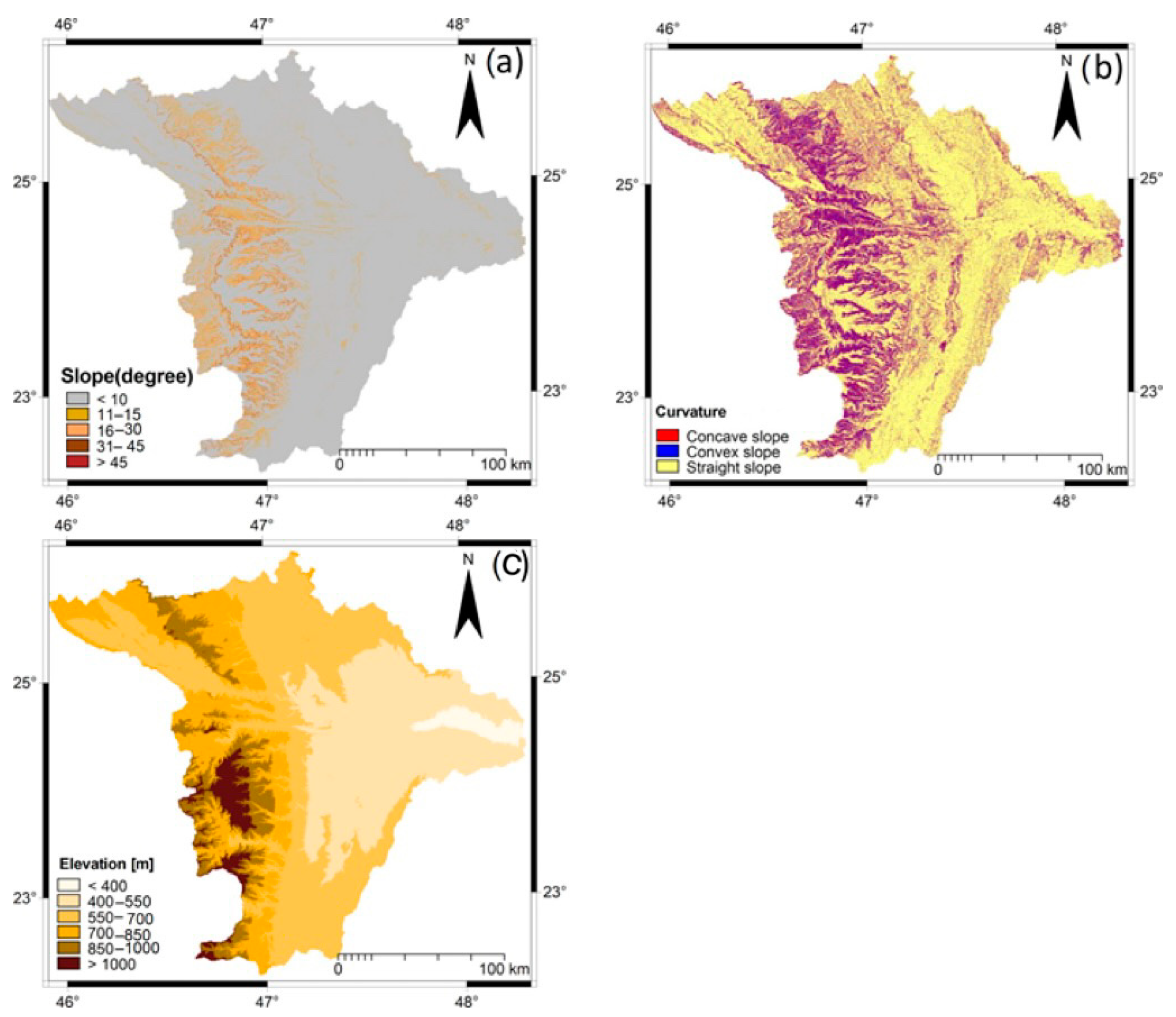
While slope angle shows the steepness of a surface for each cell, the curvature, both concave and convex, shows the change in slope angle in that cell for a short distance. The slope and curvature control the water movement within the catchment area [
10]. When the concave slope is dominant in the region, the probability of flooding is greater. However, when the convex slope is dominant, there is more time for the water to flow away to the lower slope area (concave) and accumulate. Moreover, the height of the slope indicates a lower probability of water infiltration and impermeability and hence a higher probability of flooding down the slope area. Therefore, slope and curvature are considered important factors in flood susceptibility studies [
15,
17,
23].
The slope map was then classified into five categories (using equal interval scheme) using the slicing tool of the ILWIS 3.4 GIS software (
Figure 7a). On the other hand, the curvature map was sliced into three classes: value < −0.45 for the convex area, values > 0.45 for the concave area, and values near zero for the flat area (
Figure 7b). Both maps were then assigned ratings ranging from 1 to 10. The flat areas were assigned higher values because they capture water for a long time, while areas with a steep slope were assigned lower rates because the steep slope increases the speed of water moving down.
The elevation variable was constructed by categorizing the mosaicked DEM into six classes (using an equal interval scheme) using the slicing tool of the ILWIS 3.4 GIS program (
Figure 7c). The elevation classes were then assigned ratings from 1 to 10. Flooding is more likely to occur in areas at lower altitude, as flood cannot occur in areas with high elevation [
2]; thus, high rates were assigned to areas in the low elevations category.
2.2. Method for Flood Susceptibility Analyses and Modeling
In this study, two weighted index overlay analysis methods, which have been successfully applied in many types of flood susceptibility mapping, landslide mapping, and groundwater mapping studies, were applied to generate two separate flood susceptibility maps. These methods were the weighted product model (WPM) [
82] and the analytical hierarchy process (AHP) [
5,
83].
2.2.1. The AHP Method
Based on the previously extracted variables (cf.
Section 2.2), the AHP method, developed by Saaty between 1971 and 1975 [
84], was used to map the flood susceptibility zones in the study area. This method is used to obtain an optimum solution for a complex problem in different areas of science by weighing the variables. The AHP yields a numerical index that is derived from rates and weights assigned to the independent variables. The AHP method involves the following necessary steps as descried by Kulakowski [
85]: (1) defining the overall aim of the study, (2) determining the variables related to the problem under investigation, (3) constructing a pairwise matrix to reach preferences among a set of variables towards a specific aim of the study, (4) assigning a weight for each variable according to its relative importance toward the problem under investigation using prior knowledge, (5) computing the geometric mean using a matrix analysis, and (6) computing the consistency to determine the validity of the weight assigned to each variable using a consistency ratio.
In this study, based on authors’ judgments and the relative importance, weights were assigned from 1 (less important) to 9 (more important) to all variables by constructing a pairwise comparison matrix (
Table 2). Then, scale weights were generated using eigenvalue calculation [
85]. The pairwise matrix was then normalized, utilizing the weighted arithmetic mean method, to compute the standard pairwise comparison matrix (
Table 3) as previously described [
19]. The calculation of criteria weights for all factors was then achieved by averaging the values for each row in the normalized matrix.
Subsequently, to minimize biased subjective judgments, consistency was computed using consistency index (
CI) and consistency ratio (
CR) as follows:
where
CI is the consistency index,
n is the number of variables,
CR is the consistency ratio, and
RI is the consistency index of a random index value based on many variables that are used in the pairwise matrix [
84,
86]. Using a pairwise matrix with ten variables, the RI was 1.49. For this study, the judgment made was found consistent with a
CR value > 0.1 equaling 0.03.
2.2.2. WPM Method
The weighted product model (WPM) is a technique that is commonly used to solve multi-criteria decision making (MCDM) problems [
87]. In this method, after constructing the normalized decision matrix as described in
Section 2.3.1 (cf: AHP method) through the equal weight designation to all variables, the equal weights were multiplied with the corresponding performance value in the matrix for the purpose of comparison. The weighed normalized decision matrix was then computed using Equation (9), in which equal weights were raised to the power of each performance value. Subsequently, preference scores (weights) were obtained (
Table 4) by multiplying the product of each cell with the product of the next cell. A more detailed description of this model is provided by San Cristóbal [
87].
where
Xi is the performance value and
Wi is the equal weight.
Table 5 displays the obtained variables’ classes, ratings, and weights for both the AHP and WPM methods. Finally, the flood susceptibility index (FSI) was computed by applying a linear combination of all variables with the previously obtained weights according to the following formula:
where
T,
E,
D,
Dd,
St,
G,
L,
R,
Sd, and
C are the ten variables, and the subscript w and r are the corresponding weights and rates of the variables, respectively (
Table 5). The obtained raster flood susceptibility maps were then classified (sliced) into five classes (using an equal interval scheme) with the slicing tool of the ILWIS 3.4 GIS software, which were, namely: “very low”, “low”, “moderate”, “high”, and “very high” classes. Subsequently, the total area and percentage of each susceptibility class were calculated.
2.3. Method for Accuracy Assessment
To check the applicability of the adopted models to map the flood susceptibility areas, the results (i.e., flood susceptibility maps) need to be validated, preferably using historical flood locations. In this work, the efficiency and the performance of the AHP and WPM models were verified through employing two statistical methods, as follows: (1) the area under the receiver operating characteristics (ROC) curve (AUC), and (2) the frequency ration, which is the accumulation of historical flood locations within the flood susceptibility classes.
2.3.1. ROC Curve
The area under the ROC curve (AUC) is considered one of the most efficient techniques applied to validate model results [
2,
15,
17]. It is an effective technique in medical research [
88] and machine learning and data mining studies [
89] to evaluate models’ performance effectively. It is based on a plot of the false positive rate (FPR) values or 1-specificty on the
y axis against the true positive rate (
TPR) or sensitivity on the
x axis for a set of cutoff values of the historical data to assess a model outcome as positive or negative. The AUC value varies from 0 to 1, where a value of 0 indicates minimum or poor quality of a model output and a value of 1 indicates maximum or excellent quality of a model output. The (
TPR) and (
FPT) can be calculated as follows:
where
TP (true positive),
TN (true negative),
FP (false positive), and
FN (false negative) are the correct occurrence or non-occurrence of historical flood events.
In this paper, the historical flood locations collected previously from the local sources were used (
Table 1) to compute the FPR and TPR using Equations (11) and (12), respectively. Accordingly, an ROC curve plot was designed and the area under the ROC curve (AUC) was calculated for each of the adopted flood susceptibility mapping models. These adopted models were then compared according to the differences in their performance.
2.3.2. The Identification of Flood Frequency Ration (FR) within Each Flood Susceptibility Class
We used the frequency ration approach as a second validation method to spatially relate the historical events to the flood susceptibility map’s classes, aiming to compute the frequency (density) of the historical flood points that occur within each class. For this purpose, the historical flood locations were first rasterized. The cross operation of the ILWIS 3.4 GIS software was then used to overlay the obtained flood susceptibility maps with the rasterized map. In the overlay analysis, the pixels from both maps were combined at the same locations, and the combination that resulted in each flood susceptibility class was recorded and stored in a cross table [
81]. A table aggregation function was used to obtain points (pixels) from the output cross table that was constructed within each flood susceptibility class. The flood susceptibility maps were considered valid if most (≥50%) of the historical flood locations were situated in the “moderate”, “high”, and “very high” flood susceptibility classes.
2.4. Statistical Analysis for the Optimum Flood Susceptibility Variables
A statistical analysis was carried out using a statistical package of the ILWIS 3.4 GIS software [
81]. OIF (optimum index factor) and correlation matrix operations were used to determine the most effective variables that have contributed (at most) to the flood occurrence in the study area. The OIF is a statistical index primarily developed to determine the optimum set of bands (maximum three bands) with the least correlation and highest amount of information to create a color-composite (RGB) satellite image [
81]. The OIF is expressed as follows:
where
Stdi,j,k are the standard deviations of any three rated variables, and
Corri,j,k are the correlation of the rated variables.
A correlation matrix operation was used to compute the correlation coefficients between the ten variables. The correlation coefficients are computed by following two steps; first, a covariance matrix combing all the variables is constructed, and second, the elements of the covariance matrix are normalized using the following equation [
81]:
where
Covarb1, b2 is the computed covariance of two variable layers (variable 1 and variable 2), and
var b1, b2 are the variance in the first and second variables. It was hypothesized that most of the flood susceptibility parameters are spatially invariable and correlated, which means that they contribute a little to the variance in the flood susceptibility in the study area.
2.5. The Spatial Interaction between Variable Classes and the Historical Flood Locations
Making use of the cross operation of the ILWIS 3.4 GIS software, the spatial interaction between the flood occurrence locations and the variable classes was examined. In this operation, pixels on the same position in both maps were compared using an overlay analysis. Hence, the events that occurred within each class of input variable were stored in a cross table [
81]. From this cross table, events that occurred in each class of input variable were obtained using table calculation and aggregation functions.
3. Results
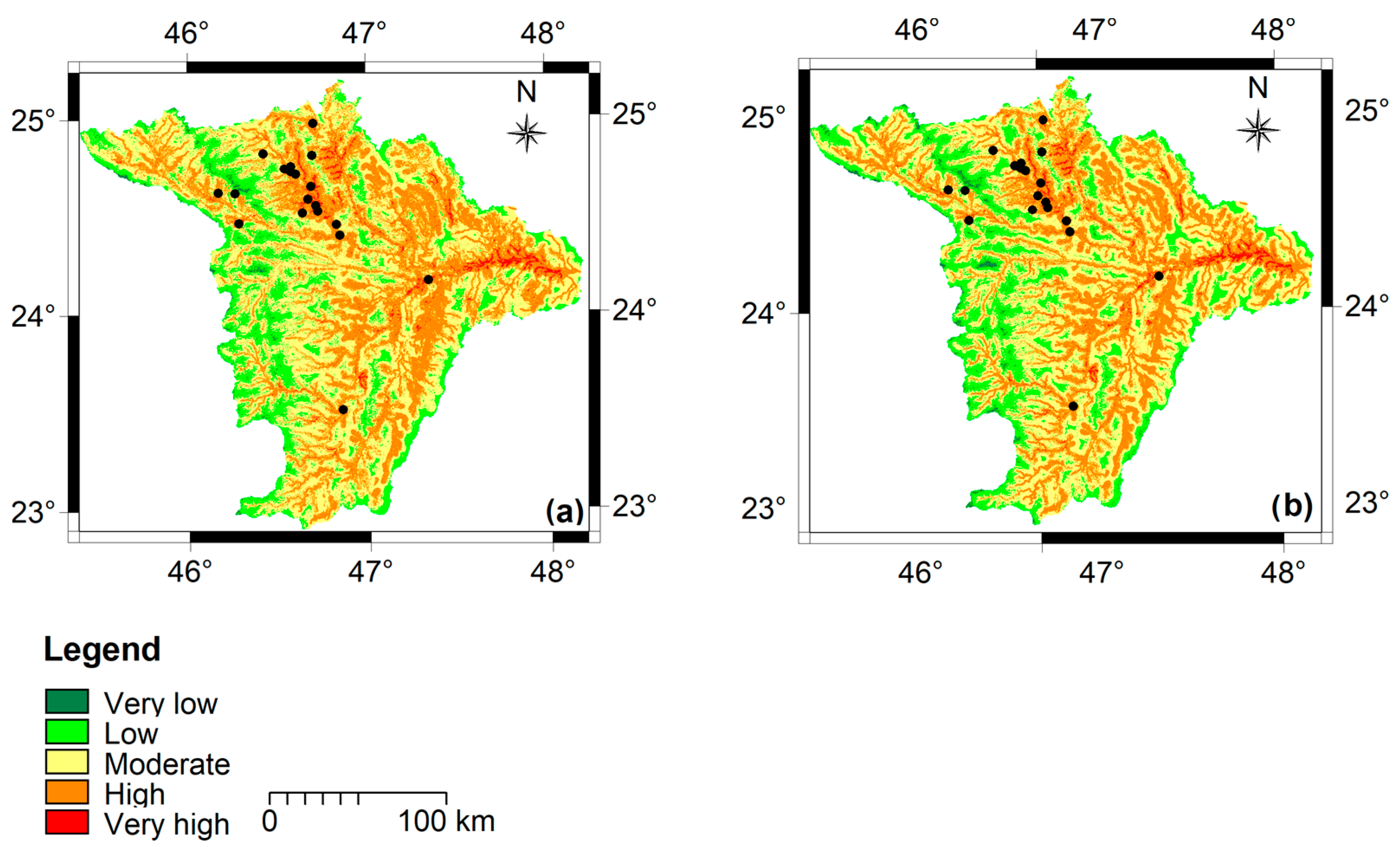
Two flood susceptibility maps were produced: the analytical hierarchy process (AHP) map (
Figure 8a) and the weighted product model (WPM) map (
Figure 8b). A comparative analysis was performed between the two maps for model validation results and the distribution of flood susceptibility zones as they were related to the ten variables.
3.1. Evaluation of Applied Models
For reliability, it is important to validate the results obtained from the two adopted models to assess their performance and efficiency. Therefore, the first step to produce the flood susceptibility maps was to test their quality and reliability by employing the two validation methods.
3.1.1. Flood Frequency Ration (Flood Density) within the Flood Susceptibility Zones
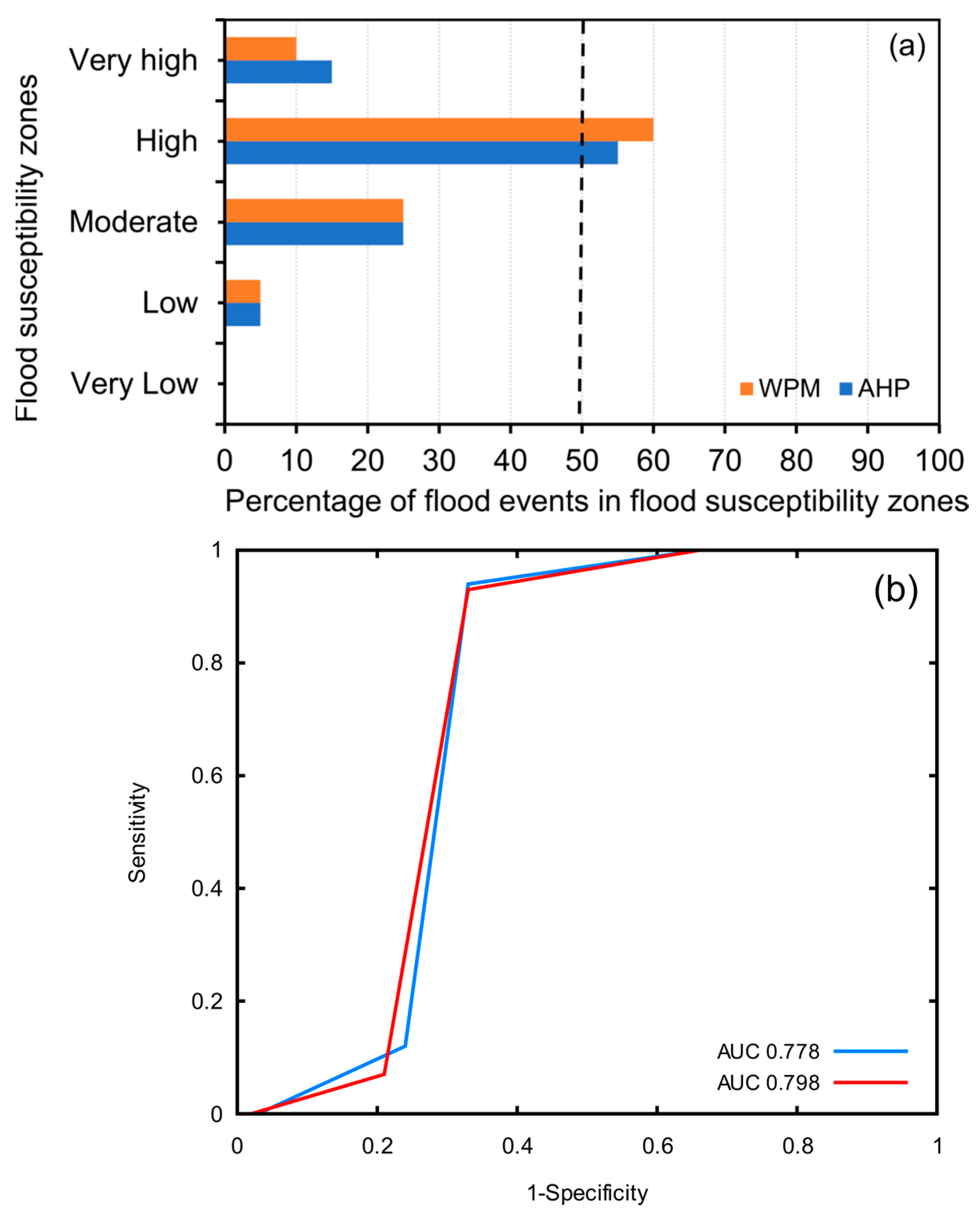
Figure 9a shows the flood frequency ration (density), computed by the cross-overly analysis operation, that occurred in each flood susceptibility class in each flood susceptibility map. Both maps displayed good agreement with the delineated high flood susceptibility zone, as the two maps slightly exceeded the specified threshold, and more than 50% of the historical flood events points were located in the high flood susceptibility zone. Regarding agreement in the moderate zone, both maps showed fair results; 25% of the points corresponded to the moderate flood susceptibility zone. In total, both maps showed significant results, with as many as 95% of the points located in moderate, high, and very high flood susceptibility zones, whereas only 5% were located in the very low and low flood zones. Additionally, the results revealed that the frequency ration (density) value gradually increased from the low to the high susceptibility class in the study area.
3.1.2. ROC Curve
Both models have shown reasonable results with an AUC of more than 77% (
Figure 9b). However, the weighted product model (WPM) had a higher predication accuracy, with an AUC of 79.8%, than the analytical hierarchy process (AHP) model, which produced an AUC of 77.8%. Therefore, it can clearly be judged that the WPM model performed better than the AHP model regarding flood susceptibility mapping.
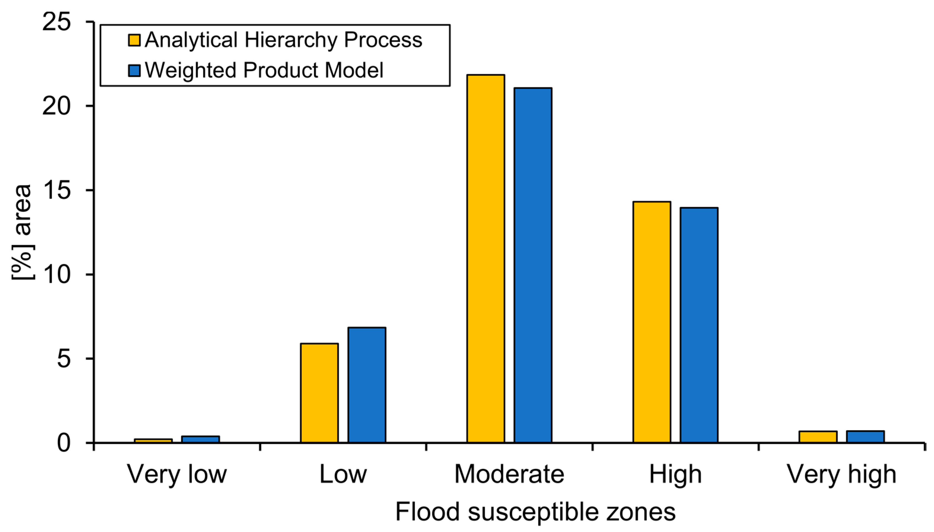
3.2. Distribution of Flood Susceptibility Zones
Five susceptibility classes were identified in the study area at a 10.916% interval for the WPM map and at a 7.592% interval for the AHP map as follows: very low, low, moderate, high, and very high (cf.
Figure 8a,b). The spatial distribution of these classes is illustrated in
Figure 10. The two-colored bars in
Figure 10 show a slight difference between the AHP and the WPM models regarding flood susceptibility classes. Both models have clearly highlighted the domination of the “moderate”, “high”, and “low” susceptibility classes in the study area. Almost half of the study area was characterized by the “moderate” susceptibility class, while the “high” susceptibility class, which occurred mainly in the northern and northeastern parts of the study area, accounted for approximately 33.34% and 32.49% of the total area, according to the AHP and the WPM models, respectively. Overall, the low susceptibility class accounted for 13.71% and 15.94% of the total area, according to the AHP and WPM models, respectively, and it was the predominant class in the high northwestern part of the study area, as shown in
Figure 8a,b.
3.3. The Importance and Relative Contribution of Variables towards Flood Susceptibility
The mean values varied considerably among the rated variables (
Table 6). The largest mean value (mean value was 9.63) was found only in one of the topographical variables, which is the slope factor. The curvature was the second variable with a medium mean value (mean value was 7.39). The TWI and elevation were characterized by lower mean values (mean values were 5.61 and 5.52, respectively) in comparison with the slope and curvature variables. The distance to the drainage network (hydrologic variable) and land use/land cover (environmental variable) were characterized by lower mean values (mean values were < 4). The Dd (hydrologic variable) was characterized by a medium mean value (mean value was 7.01), followed by the runoff (Q) variable with its lowest mean value (mean value was 5.96), compared with the other hydrologic variables. The geology (environmental variable) was characterized by a high mean value (mean value was 8.18) compared with the soil type variable, which had a medium mean value (mean value was 7.31) (
Table 6).
The “land use/land cover”, “runoff”, and “soil type” parameters were observed to be highly variable (CV% were 48.6, 48, and 46.2, respectively), while the “distance to the drainage network”, “elevation”, “curvature”, and “Dd” parameters were moderately variable (CV% were 36.2, 35.1, 32.3, and 31.1, respectively). The “geology”, “TWI” and “slope” parameters were the least varying factors (CV% was 25.6, 23, and 12, respectively). Overall, a low variability indicates that the parameter has a weak contribution to the variation in the flood susceptibility index across the study area.
The result of the correlation analysis is presented in
Table 7 (only statistically significant correlation coefficients are reported here). We found a strong correlation between the land use/land cover and runoff (Q) (r = 0.72), unlike the slope correlation with TWI and elevation, where weak correlations (r = 0.31 and 0.30, respectively) were exhibited. The most robust negative correlation was observed between the elevation and geology (r = −0.51). The geology and runoff, the distance to the drainage network, and Dd showed the least correlations (r = 0.28 and 0.25, respectively). However, the variables were considered virtually independent (
Table 7).
According to the OIF rank results, the best combination of factors dictating the variability in the flood occurrence within the study area were geology, land use/land cover, and soil type, as these factors had the highest amount of standard deviation and the lowest correlation.
The analysis of the land use/land cover map (
Figure 5a) revealed that the bare exposed rock mostly dominated over the study area; it represented 36.79% (27,851.4 km
2) of the total area, primarily in the center. The remaining 63.21% (5045.2 km
2) was dominated by the other land use/land cover classes (i.e., urban, agriculture, and shrub). The dominant geological features in the study area were Jurassic and Cretaceous. Jurassic features accounted for 19.93% (15,084.7 km
2) of the area, while Cretaceous features accounted for 12.24% (9266.03 km
2), primarily extending from the eastern part toward the center and from the western part toward the center (
Figure 5c). The Calcic Yermosols soil type was found in the study area and accounted for 24.73% (18,723.6 km
2). The sandy loam and loamy sand were the major soil textures in the study area. They accounted for 51.62% (16,982.67 km
2) and 31.61% (10,398.4 km
2) of the area, respectively. In addition, it was found that 65.76% (21,634.1 km
2) of the total area was covered by the hydrological soil group “B”, which is characterized by a medium infiltration rate whereas, and about 31.61% of the total area was covered by soil group “A”, which is characterized by a high infiltration rate. The remaining 2.63% of the area was represented by the hydrological soil group “C”, which is characterized by a low infiltration rate, and it was mainly concentrated in the center of the study area, where the main land use was mostly urban and agriculture.
Most of the study area was dominated by “moderate” elevation values. The elevation in the study area decreases gradually from west to east, and this decrease has made the eastern part more susceptible to flooding. The “moderate” elevation—ranging between 550 and 700 m—was 12,240.97 km2 and accounted for 37.2% of the total area. The area characterized with “high” and “very high” values both accounted for 12.03% of the total area. Similarly, the slope maintains a gentle grade (<10°) throughout most of the study area, and it mostly increases toward the west, northwest, and southwest, which is associated with the availability of some scattered mountains. The areas with a steep slope (>45°) accounted for 0.17% (54.8 km2), while the gentle slope represented the majority of the study area, with 89.23% (29,274.56 km2); thus, it was typically assigned a high rating score, indicating its highest effects on the occurrence of floods. Similarly, the “moderate” category of the TWI was prevalent in the study area, accounting for 56.55% (18,554.36 km2) of the area.
The morphometric analysis revealed that the study area was naturally served by a drainage area of about 32,897.24 km2, had a channel length of 376,149 m, had an average channel slope of 0.9%, and had an average slope steepness of 40.6%. The study area had six drainage orders, where the first order constituted 77.8% of the total stream network with a length of 3999.84 km and bifurcation ratio (Rb) of 5.65. Moreover, the stream network had a mean bifurcation ratio (Rbm) of 4.95, mean stream length of 649.2 m, and stream frequency of 0.018. In addition, the study area was characterized by low Dd (0.18–0.36 km/km2). The western part of the study area had relatively very low Dd (<0.18 km/km2). The total area covered by the “low” and “very low” Dd was 8269.6732 km2, accounting for 25.42%, and 21,006.61 km2, accounting for 64.58% of the total area, respectively.
Most of the study area was characterized by “high” runoff (Q) (2.3 to >3.3 mm), and it constituted 58.9% (19,387.41 km2) of the total study area. It has been noticed that the “very high” runoff (Q) rate (>3.3) mm was primarily concentrated in the area covered by urban land use, and accounted for only 3.4% (1129.34 km2) of the total area. The area characterized by “very low” runoff (Q) was 10,395.33 km2, accounting for 31.6% of the total area, primarily in an area covered by sand.
3.4. The Spatial Interaction between Flood Susceptibility Variable Classes and Historical Flood Locations
The results obtained from the cross operation between the classes of the sliced variables and the historical flood event locations are summarized in
Table 8. The results indicate that areas with a slope <10 degrees has the highest accumulation of flood occurrence locations, and about 95% of the historical flood events have occurred in this class. The accumulation of flood occurrence locations decreased when slope degrees increased. The results regarding the curvature variable showed that about 75% of the flood occurrence events have occurred in areas characterized by flat curvature, followed by concave curvature with only 15%. The elevation results showed that the highest percentage (about 75%) of the flood occurrence events accumulated in elevation classes ranging between 550 and 700 m. With regard to the geological variables, about 80% of the historical flood locations are places characterized by Jurassic formations. Concerning the class of soil type, Calcic Yermosols had the highest accumulation of flood occurrence, with 55%, followed by Calcar ic Regosols, with 30%, while only 15% have occurred in areas characterized by the Cambic Arenosols soil type. About 75% of the floods have occurred in areas characterized by hydrological soil group (HSG) “B”, while nearly 25% have occurred in areas with HSG “C”. With respect to the results of the land use/cover variable, urban areas and bare exposed rock had the highest percentage of flood occurrence, with values of 45% and 40%, respectively. Regarding the results of the Dd variable, the highest percentage (60%) of floods have occurred in areas with Dd ranging between 0.18 and 0.36; whereas nearly 40% have occurred in areas characterized by a Dd of <0.18. With regard to the runoff (Q) parameter results, about 90% of the flood events occurred in areas characterized by runoff (Q) ranging between 2.3 and >3.3 mm. The results regarding the distance from the drainage network parameter showed that 90% of the floods have taken place within distances ranging between 0 and 3000 m. Furthermore, the analysis of the TWI results showed that the highest accumulation of flood occurrence occurred in two classes: 5–10 and 10–15, and about 90% of the historical flood events have occurred in these two classes.
5. Conclusions
In this paper, an attempted to map and evaluate flood susceptibility zones in the Wadi Hanifah drainage basin using the AHP and WPM models. Remote sensing data from Landsat-8, Shuttle Radar Topography Mission (SRTM), and other additional datasets were used to map ten relevant variable categories (topographical, hydrological, and environmental), including: the distance to the drainage network, elevation, land use/land cover, runoff, slope, curvature, geology, soil type, Dd, and TWI. A correlation matrix and OIF were used to determine the most important variables that contribute (the most) to the occurrence of floods. We successfully validated the AHP and WPM maps using historical flood event locations and the FR and AUC methods. The main results are summarized as follows:
Substantially, the study findings confirmed that it is better to use the WPM model, as it provides a better accuracy than the AHP model.
The obtained flood susceptibility maps indicated that 33% of the total land area was dominated by the “high” risk class, primarily in the north and northeastern parts of the study area, whereas 50% was dominated by “moderate” class, where the slope (mean importance: 9.63), followed by the geology (mean importance: 8.18), were determined to be the main factors controlling the occurrence of floods.
In addition, the elevated western part of the study area comprised mainly “very low” and “low” flood susceptibility zones, accounting for 0.49% and 13.71% of the total area, respectively.
Moreover, we noticed that the distance to the drainage network was the least important variable, with a mean importance of 3.73, followed by land use/land cover (mean importance: 3.83).
The analysis of the OIF indicated that the most important information about flood occurrence in the study area can be provided by three variables, namely: geology, land use/cover, and soil type. These variables were characterized by the least amount of duplication, i.e., the lowest correlation among the map pairs, and the highest sum of the standard deviation.
Finally, most notably, this study contains promising results on our knowledge regarding mapping and evaluating flood susceptibility areas. However, some limitations are worth noting. Although the obtained results have been validated in practice, the sample does not represent the whole region. Furthermore, most of the variables (topographical, hydrological, and environmental) were extracted from medium-resolution remote sensing data (~30 m), which could result in lower flood prediction precision. In addition, the weight assigned to each variable was subjective. In future investigations, mapping and evaluating flood susceptibility using parameters derived from LiDAR data using advanced machine learning techniques, such as random forest (RF) or support vector machine (SVM), is recommended to obtain a deeper understanding of flood susceptibility risk and control in the Riyadh region. We emphasize that the results obtained from this study represent a useful tool for local government and organizations, which are working on flood control and mitigation, to reduce flood risk through early flood risk management, as they can use these results as a guide to identify areas with high potential risk that must be avoided by the residing population.


