A Novel Energy Performance Prediction Approach towards Parametric Modeling of a Centrifugal Pump in the Design Process

Abstract

Traditional centrifugal pump performance prediction (CPPP) employs the semi-theoretical and semi-empirical approaches; however, it can lead to many prediction errors. Considering the superiority of deep learning when applied to nonlinear systems, in this paper, a method combining hydraulic loss and convolutional neural network (HLCNN) is applied to CPPP. Head and efficiency were selected as two variables for demonstrating the energy performance of the centrifugal pump in order to reflect the prediction ability of the proposed model. The evaluation results indicate that the predicted head and efficiency are accurate, compared with the experimental results. Furthermore, the HLCNN prediction model was compared against machine learning methods and the computational fluid dynamic method. The proposed HLCNN model obtained a better ARE_mean, root mean square error, sum of squares due to error, and mean absolute error for centrifugal pump energy performance. The research revealed that the HLCNN model achieves accurate energy performance prediction in the design of centrifugal pumps, reducing the development time and costs.

1. Introduction

In general, the research on centrifugal pumps mainly focuses on four stages: design and development, manufacturing, performance testing, and optimization and improvement [1]. This paper focuses on extracting feature information and predicting energy performance according to critical design and operation parameters of the centrifugal pump during the first stage only, with the goal of shortening the development period and reducing research costs. Current methods of centrifugal pump performance prediction (CPPP) mainly include the hydraulic loss method (HLM) [2,3,4,5], the computational fluid dynamic (CFD) [6,7,8] numerical simulation method, and the artificial neural network (ANN) method [9,10,11,12].

Because it takes into consideration factors such as secondary flow, the HLM is widely used in the field of CPPP. Lin [13] applied the enstrophy dissipation method to study hydraulic loss, and the results showed that the losses are controlled by the fluctuating and the wall enstrophy dissipation power. Naggar [14] used Euler and energy equations to calculate the fluid slip and volute loss at the impeller outlet. However, due to the difference in hydraulic loss between the mathematical calculation models for different types of pumps, the application is subject to restrictions. The development of computer visualization technology has led to the CFD method being widely used in the research on various fluid machineries [15,16,17,18]. Kang [19] used CFD to predict the variation rule of internal flow and performance parameters of the short blade centrifugal pump. Rehman [20] used ANSYS soft to predict the cavitation phenomenon of the pump under different working conditions. However, CFD’s effectiveness in prediction accuracy depends to a certain extent on the engineers’ experience. In recent years, ANNs have been increasingly used to predict complex behavior in uncertain problems [21,22,23]. Zhao [24] combined the gray clustering method and a second curvelet neural network to predict the performance ratio of photovoltaic pumping systems. The simulation results showed that the second curvelet neural network had the highest prediction precision. Mrinal [25] developed approximate models based on ANN to predict pump performance. These approximation models can eliminate the expensive testing to plot the performance curve of a pump. Park [26] applied ANN to predict the seasonal heating performance of a large-scale ground-source heat pump system. The prediction model can be used as a baseline for the measurement and verification of future energy conservation measures and real-time performance monitoring to check for system malfunctions. Nie [27] used a back-propagation neural network (BPNN) algorithm to predict centrifugal pump performance and found that the errors of head and efficiency were 7% and 8%, respectively. Deng [28] used the least squares support vector regression (LSSVR) algorithm to predict pump performance from multiple impeller parameters but did not consider the influence of volute parameters. Although the above findings have achieved good results, they have one drawback: only one hidden layer was selected in the structure of the prediction model, and the features contained in the training data were not always completely extracted. The reason why only one hidden layer was selected is that, for these shallow networks, due to the particularity of the training algorithm, a large number of hidden layers might cause difficulty in the training process, and they are prone to problems such as overfitting, gradient disappearance, and falling into local minimum value [29]. Therefore, an ANN with one hidden layer was unable to extract pump features efficiently, and the prediction accuracy of the pump needed to be further improved.

Later, with the rapid development of computer software and hardware technology, deep learning (DL) has been proven to alleviate the problems of training difficulties and gradient disappearance caused by the shallow neural network algorithm [30]. Several researchers have introduced convolutional neural networks (CNNs) in DL to performance prediction in various fields [31,32,33]. CNNs have been shown to outperform ANNs with one hidden layer and learn features automatically instead of requiring manual design [34,35]. Ye [36] used a CNN to predict the pressure coefficient of a non-uniform cylindrical flow, and prediction accuracy was significantly improved. Harbola [37] used a one-dimensional CNN to predict the dominant wind speed and direction of the wind field; these research results are beneficial for the installation of wind turbines. Haidar [38] used a deep CNN to predict the monthly rainfall of a location in eastern Australia. Yong [39] introduced DL to quantitatively predict changes in the heating capacity, power consumption, and performance coefficient of air source heat pumps. DíazeVico D [40] used a CNN to predict wind energy and solar irradiance, based on input data from a numerical weather prediction system. These results attest to the powerful feature extraction ability of the CNN.

However, most researchers using deep neural networks for performance prediction only migrated the DL directly from other fields, including CPPP, without considering the embedding of physical laws between the design and performance parameters of centrifugal pumps for small datasets. In this paper, we did consider this correlation in exploring a new method suitable for CPPP and validated it by carrying out experiments. The novelty of this approach is that it predicts centrifugal pump performance based on HLM and CNN (HLCNN), rather than relying solely on a purely data-driven black box agent model to complete CPPP. In addition, for the centrifugal pump’s entire flow field, the performance prediction process considered hydraulic loss analysis, giving it the advantage of improving the interpretability and stability of the intelligent model.

Therefore, to improve the accuracy and interpretability of the CPPP model under small sample datasets, this paper proposes a HLCNN-based approach for predicting the energy performance of a centrifugal pump. This paper achieved the CPPP by using multiple alternately distributed convolutional layers to complete the adaptive learning of performance features and combine the fully connected layer (FCL). The main contributions are as follows: (1) a hybrid CPPP model considering the relationship between centrifugal pump hydraulic loss and energy performance is established; (2) considering the influence of network structure on the CPPP model, the feature learning speed of different convolutional layers is analyzed; and (3) compared with an experimental study and other methods (BPNN, LSSVR, CFD), the effectiveness of the proposed model is proved.

2. Methodology and model

2.1. Modeling of Hydraulic Loss and Energy Performance of Centrifugal Pump

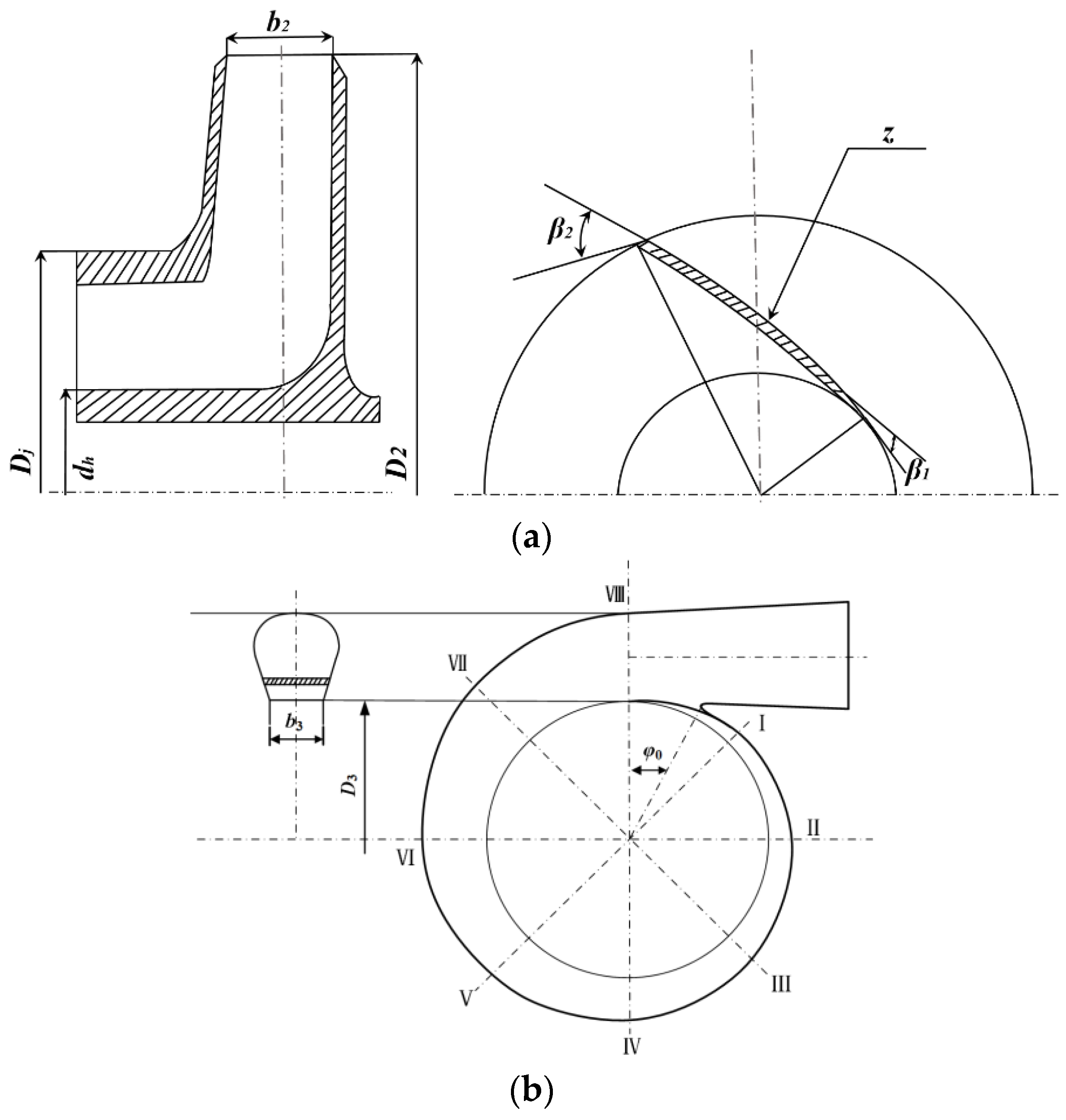
The common structure of a centrifugal pump consists of inlet, impeller, volute, and outlet. The impeller and volute play the crucial role in energy conversion in a centrifugal pump. The main design parameters of the impeller and volute are shown in Figure 1, including the impeller inlet diameter (D_j), impeller outlet diameter (D₂), blade outlet width (b₂), the number of blades (z), blade outlet angle (β₂), hub diameter (d_h), blade inlet angle (β₁), volute base circle diameter (D₃), and volute inlet width (b₃), initial angle of volute tongue (φ₀), and throat area (F_t). The specific speed (n_s), flow rate (Q), and impeller rotational speed (n) are significant operating parameters of the pump. The design and operating parameters affecting the centrifugal pump energy performance (head (H) and efficiency (ղ)) have been widely researched [41,42,43].

Generally, there are many semi-theoretical and semi-empirical methods to calculate the hydraulic loss of a centrifugal pump. Hydraulic loss is mainly caused by the inlet, impeller, and three volute parts, and the inlet is usually ignored. In this section, the following hydraulic losses are taken into consideration: (a) impeller inlet shock loss (l_iis), (b) impeller surface friction loss (l_isf), (c) impeller flow passage diffusion loss (l_ifd), (d) volute inlet shock loss (l_vis), (e) volute friction loss (l_vfri), and (f) volute diffusion loss (l_vdif).

2.1.1. Impeller Inlet Shock Loss

When the centrifugal pump operates under off-design conditions, shock loss will occur at the blade inlet. The l_iis depends on the relative velocity of the blade inlet, which is defined as:

$$l_{\mathrm{iis}}=\frac{f_{\mathrm{iis}}}{2g}{(u_1\frac{Q-Q_{\mathrm{d}}}{Q_{\mathrm{d}}})}^2$$

(1)

where f_iis is the impeller inlet shock loss coefficient, u₁ is the circumferential velocity of the impeller inlet, and Q_d represents the flow rate of the centrifugal pump under design conditions.

2.1.2. Impeller Surface Friction Loss

The impeller surface friction loss follows that of the standard pipe friction model [44], and the corrected l_isf is as follows:

$$l_{\mathrm{isf}}=z{k}_3{\lambda }_1\frac{l_{\mathrm{a}}}{D_{\mathrm{a}}}\frac{w_{\mathrm{a}}{}^2}{2g}$$

(2)

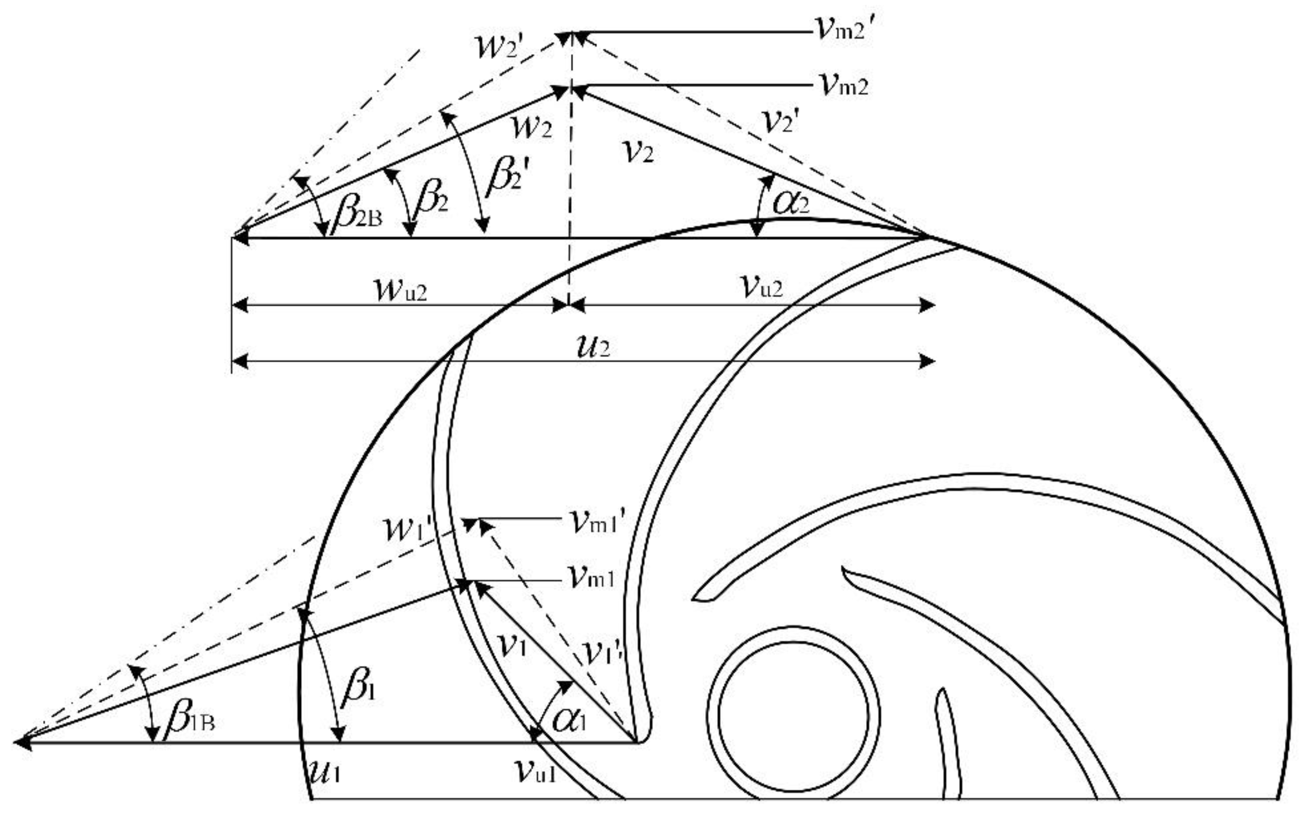
The relationship between impeller circumferential velocity (u), relative velocity (w), and absolute velocity (v) is obtained from the rules of vector addition, which can be illustrated as velocity triangles [45]. The relevant parameters used in this work to calculate the l_isf are presented in

Table 1. Relevant parameters of impeller surface friction loss.

Parameter	Expression
k3: impeller friction loss correction coefficient	$k_3=1/4.68n_{\mathrm{s}}{}^{0.0185}-4.84$	(3)
λ1: impeller linear friction coefficient	${\lambda }_1={\left[1.74+2\lg (D_{\mathrm{a}}/2\delta )\right]}^{-2}$	(4)
la: hydraulic length of the flow passage	$l_{\mathrm{a}}=(D_2-D_{\mathrm{j}})/(\sin {\beta }_2+\sin {\beta }_1)$	(5)
Da: average diameter of the flow passage	$D_{\mathrm{a}}=(D_2+D_{\mathrm{j}})/2$	(6)
wa: average relative velocity	$w_{\mathrm{a}}=0.5(w_1+w_2)$	(7)

Here, δ is the surface roughness of the centrifugal pump. w₁ and w₂ are the relative velocity of the impeller inlet and outlet.

.

2.1.3. Impeller Flow Passage Diffusion Loss

When liquid flows through the centrifugal pump, it will cause flow separation on the impeller inner wall, which is defined as:

$$l_{\mathrm{ifd}}=0.25\frac{w_1{}^2}{2g}$$

(8)

2.1.4. Volute Inlet Shock Loss

When the centrifugal pump operates under off-design conditions, the liquid that flows out of the impeller and enters the volute will have an impact due to the different velocity, which is shown as:

$$l_{\mathrm{vis}}={\left(\frac{v_{\mathrm{m}2}}{u_2}\right)}^2{\left(\frac{1}{{\mathsf{\psi }}_2}-\frac{b_2}{b_3}\right)}^2$$

(9)

where u₂ and v_m2 are the circumferential and axial velocities at the impeller outlet, and ψ₂ is the extrusion coefficient of the blade outlet.

2.1.5. Volute Friction Loss

According to the theory of equivalent pipe flow loss [46], the l_vfri can be estimated as:

$$l_{\mathrm{vfri}}=k_7{\lambda }_2\frac{l{v}_{\mathrm{a}}}{D\times 2g}$$

(10)

The relevant parameters used in this work to calculate the l_vfri are presented in

Table 2. Relevant parameters of volute friction loss.

Parameter	Expression
k7: volute friction loss correction coefficient	$k_7=-0.071+6.3\frac{n_{\mathrm{s}}}{100}-2{(\frac{n_{\mathrm{s}}}{100})}^2-3.44{(\frac{n_{\mathrm{s}}}{100})}^3+1.7{(\frac{n_{\mathrm{s}}}{100})}^4$	(11)
λ2: volute linear friction coefficient	${\lambda }_2={\left[1.2+2\lg (D/2\delta )\right]}^{-2}$	(12)
l: equivalent tube length of volute	$l=\mathsf{\pi }\left(1-{\phi }_0/360\right)\left(D_3+D\right)$	(13)
D: equivalent tube diameter of volute	$D=\sqrt{\frac{2F_{\mathrm{t}}}{\mathsf{\pi }}}$	(14)

Here, v_a is the average velocity in the volute.

.

2.1.6. Volute Diffusion Loss

As the volute flow passage is in a diffusion state, the diffusion loss of the liquid flow out of the impeller and entering the volute is calculated as follows:

$$l_{\mathrm{vdif}}=C_{\mathrm{v}}\frac{v_{3\mathrm{d}}{}^2}{2g}$$

(15)

C_v is the volute loss coefficient. v_3d is the velocity component in a tangential direction to the impeller.

To sum up, the actual head (H) and total efficiency (ղ) of the centrifugal pump in this paper can be expressed as:

$$H=H_{\mathrm{t}}-(l_{\mathrm{iis}}+l_{\mathrm{isf}}+l_{\mathrm{ifd}})-(l_{\mathrm{vis}}+l_{\mathrm{vfri}}+l_{\mathrm{vdif}})$$

(16)

$$\eta ={\eta }_{\mathrm{h}}{\eta }_{\mathrm{v}}{\eta }_{\mathrm{m}}$$

(17)

$${\eta }_{\mathrm{h}}=H/H_{\mathrm{t}}$$

(18)

$${\eta }_{\mathrm{v}}=1/(1+0.68n_{\mathrm{s}}{}^{-2/3})$$

(19)

$${\eta }_{\mathrm{m}}=1-0.07/{(n_{\mathrm{s}}/100)}^{7/6}$$

(20)

Here, H_t, ղ_h, ղ_v, and ղ_m are the theoretical head, hydraulic efficiency, volumetric efficiency, and mechanical efficiency of the centrifugal pump [47]. The theoretical calculation of H_t (as shown in Appendix A) can be referred to the literature [48].

2.2. Hydraulic Loss–Convolution Neural Network (HLCNN)

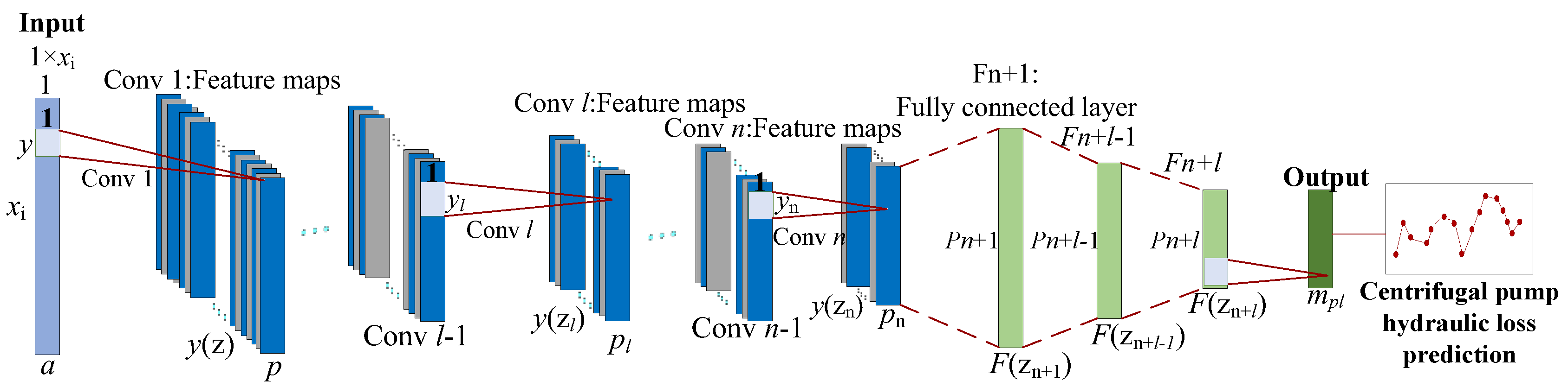
CNN is an end-to-end, supervised neural network, whose basic structure can be divided into input layer, alternately distributed convolutional layer, pooling layer, FCL, and output layer. In this paper, the basic architecture for predicting the hydraulic loss of the centrifugal pump applying the CNN is shown in Figure 2. In addition, the nonlinear mathematical relation between centrifugal pump design, operation parameters, and hydraulic loss can be derived as follows.

First, suppose that the input layer neuron is a (aϵx_i), which represents the design and operation parameters of the centrifugal pump. The expression of the centrifugal pump feature information g(z) extracted from the first convolution layer (Conv1) through p channels is shown in Equation (21), where $w_{\mathbf{1},\mathbf{y},\mathbf{z}}^{\mathbf{z}}$ is the convolution kernel and b^z is the bias of the Conv1.

$$\mathit{g}\mathbf{(}\mathit{z}\mathbf{)}={\displaystyle \sum _{y=1}^i{\displaystyle \sum _{z=1}^p{a}_{1,y,1}}}\times {\mathit{w}}_{\mathbf{1},\mathbf{y},\mathbf{z}}^{\mathbf{z}}+{\mathit{b}}^{\mathit{z}},z=1,2\dots p$$

(21)

After each channel completes the convolution computation, the nonlinear transformation is conducted by applying the rectified linear unit (ReLU) [49], and the output of Conv1 is given by

$$\mathit{y}(\mathit{z})=f(\mathit{g}(\mathit{z}))=\max \left\{0,\mathit{g}(\mathit{z})\right\},z=1,2\dots p$$

(22)

Assuming that the CPPP model in this paper contains n convolutional layers, the feature information extracted through the n-th convolution layer (Convn) is presented in Equation (23). The output of Convn is shown in Equation (24).

$$\mathit{g}({\mathit{z}}_{\mathit{n}})={\displaystyle \sum _{y_n=1}^k{\displaystyle \sum _{z_n=1}^{p_n}{\mathit{a}}_{\mathbf{1},{\mathbf{y}}_{\mathbf{n}},{\mathbf{z}}_{\mathbf{n}}}^{{}^{\mathbf{n}-1}}}}\times {\mathit{w}}_{\mathbf{1},{\mathbf{y}}_{\mathbf{n}},{\mathbf{z}}_{\mathbf{n}}}^{{\mathbf{z}}_{\mathbf{n}}}+{\mathit{b}}^{{\mathbf{z}}_{\mathbf{n}}}$$

(23)

$$\mathit{g}({\mathit{z}}_{\mathbf{n}})={\displaystyle \sum _{y_n=1}^k{\displaystyle \sum _{z_n=1}^{p_n}{\mathit{a}}_{\mathbf{1},{\mathbf{y}}_{\mathbf{n}},{\mathbf{z}}_{\mathbf{n}}}^{{}^{\mathbf{n}-\mathbf{1}}}}}\times {\mathit{w}}_{\mathbf{1},{\mathbf{y}}_{\mathbf{n}},{\mathbf{z}}_{\mathbf{n}}}^{{\mathbf{z}}_{\mathbf{n}}}+{\mathit{b}}^{{\mathbf{z}}_{\mathbf{n}}}$$

(24)

Next, the centrifugal pump feature information extracted from n convolutional layers is inputted to the first fully connected layer (FCL1), and the output of FCL1 is shown in Equation (25), where f₁ represent the number of neurons of FCL1. Similarly, the feature information of the (n + l)th layer is inputted to the regression layer, and the regression function is shown in Equation (26), where w^T and b are regression coefficients.

$$\mathit{F}({\mathit{z}}_{\mathbf{n}+\mathbf{1}})={\displaystyle \sum _{i=1}^{f_1}{\displaystyle \sum _{y_{n+1}}^q{\displaystyle \sum _{z_{n+1}}^{p_n}{\mathit{a}}_{\mathbf{1},{\mathbf{y}}_{\mathbf{n}+\mathbf{1}},{\mathbf{z}}_{\mathbf{n}+\mathbf{1}}}^{{}^{\mathbf{n}}}\times {\mathit{w}}_{\mathbf{1},{\mathbf{y}}_{\mathbf{n}+\mathbf{1}},{\mathbf{z}}_{\mathbf{n}+\mathbf{1}}}^{{\mathbf{z}}_{\mathbf{n}+\mathbf{1}}}+{\mathit{b}}^{{\mathbf{z}}_{\mathbf{n}+1}}}}}$$

(25)

$$e(x)=w^{\mathrm{T}}x+b$$

(26)

Finally, all feature information of the centrifugal pump is outputted from the output layer, as shown in Equation (27), where m_pl represents all hydraulic loss of the centrifugal pump.

$${\mathit{m}}_{\mathbf{p}\mathbf{l}}=e(\mathit{F}({\mathit{z}}_{\mathbf{n}+\mathbf{l}}))$$

(27)

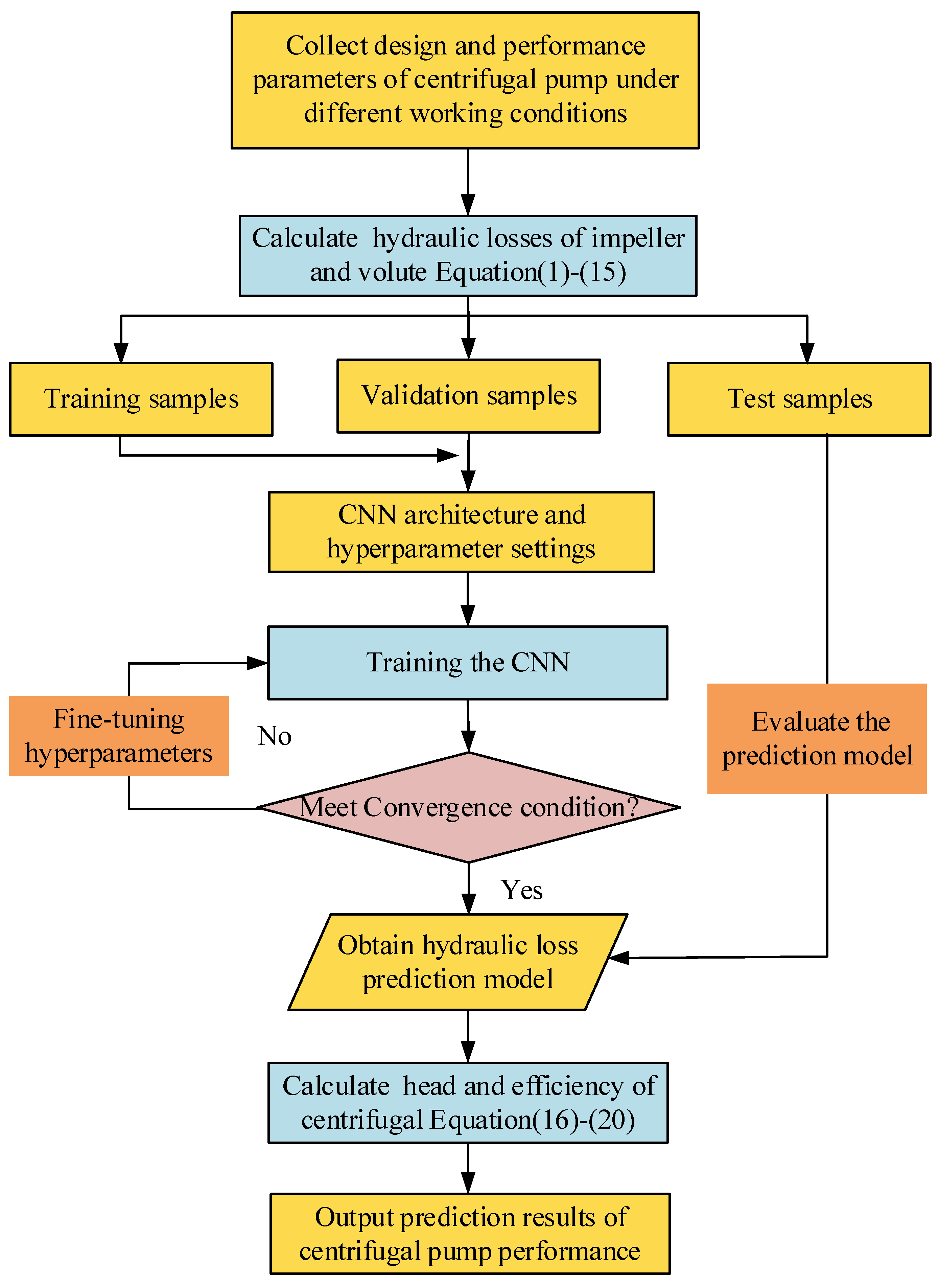
As can be seen in Figure 3, the prediction process consisted of three parts. The first part was to calculate the hydraulic loss of the impeller and volute based on the design and operation parameters of the centrifugal pump.

The second part was to build a fully convolution neural network. To improve the stability of the network and avoid the gradient disappearance in the training process, all activation functions were set as ReLUs. The Adam algorithm [50] was used to optimize and update each training parameter. To accelerate the learning speed of centrifugal pump feature information and ensure the correctness of the training direction, mapminmax normalization was used to initialize the training samples.

The third part was the evaluation of the HLCNN model. The test samples were inputted to the prediction model for testing, and the prediction model was evaluated by comparing the absolute relative error (ARE) between the predicted and the experimental values, as follows:

$$\mathrm{ARE}=\frac{\left|{\mathit{y}}_{\mathbf{i}}-{\widehat{\mathit{y}}}_{\mathbf{i}}\right|}{{\mathit{y}}_{\mathbf{i}}}$$

(28)

Other regression evaluation indicators [51], including root mean square error (RMSE), the sum of squares due to error (SSE), and mean absolute error (MAE) are defined as follows:

$$\mathrm{RMSE}=\sqrt{\frac{1}{n}{\displaystyle \sum _{\mathrm{i}=1}^{\mathrm{n}}{\left({\mathit{y}}_{\mathbf{i}}-{\widehat{\mathit{y}}}_{\mathbf{i}}\right)}^2}}$$

(29)

$$\mathrm{SSE}={\displaystyle \sum _{\mathrm{i}=1}^{\mathrm{n}}{\left({\mathit{y}}_{\mathbf{i}}-{\widehat{\mathit{y}}}_{\mathbf{i}}\right)}^2}$$

(30)

$$\mathrm{MAE}=\frac{1}{n}{\displaystyle \sum _{\mathrm{i}=1}^{\mathrm{n}}\left({\mathit{y}}_{\mathbf{i}}-{\widehat{\mathit{y}}}_{\mathbf{i}}\right)}$$

(31)

where y_i and ŷ_i represent the experimental and predicted values of the i-th sample, and n is the number of samples.

The HLCNN model framework used to predict the hydraulic loss of centrifugal pump is shown in Figure 4.

3. Experimental Research and Data Sources

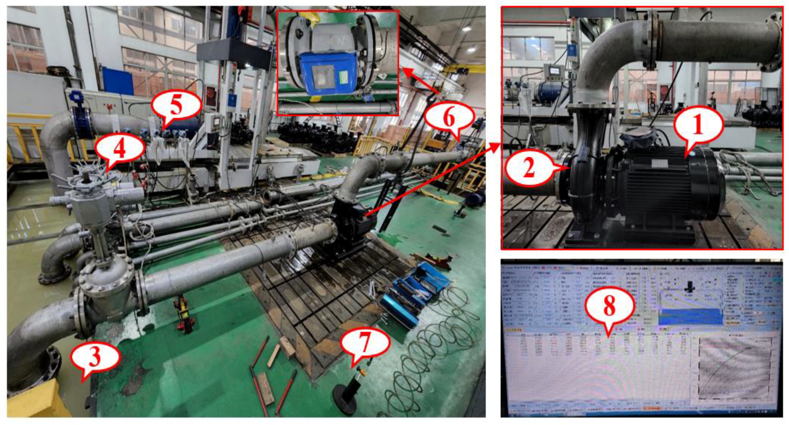
The centrifugal pump is an indispensable energy conversion machine on pump station systems. The prediction of its energy performance directly affects the energy-saving transformation and stable operation of the pump station system. In order to study the relationship between the energy performance and design parameters of the centrifugal pump, performance tests were carried out on an open test rig in Zhejiang, China. The test rig met the Chinese national standard of GB/T3216, and the test accuracy was Level I. The working medium was room temperature water. The experimental devices for the energy performance test are presented in Figure 4. Two pressure sensors were installed at the inlet and outlet pipe of the centrifugal pump. The flow rate was controlled by an electric valve, and a photoelectric sensor was used for feedback on the impeller rotational speed. Finally, the obtained energy performance parameters were saved and processed in real time by the data acquisition system.

In this paper, the fourteen design parameters, namely D_j, D₂, b₂, z, β₂, d_h, β₁, D₃, b₃, φ₀, F_t, and n_s, Q, and n are considered as the input variables of the HLCNN model. The six hydraulic losses, namely l_iis, l_isf, l_ifd, l_vis, l_vfri and l_vdif, were selected as output variables. In the design of the centrifugal pump, the variations in these parameters were related to each other along with the working condition and the regulation mode. In this paper, the HLCNN model is proposed to predict the head and efficiency of the centrifugal pump. Consequently, the modeling samples of the centrifugal pump can be represented as M = {X, Y}, where X = [x₁, …, x_N]^T∈R^n×14, Y = [y₁, …, y_N]^T∈R^n×6, and n is the number of the sampling set. The i-th sample set can be further described as m_i = {(x_i = [D_j (i), D₂(i), b₂(i), z(i), β₂(i), d_h(i), β₁(i), D₃(i), b₃(i), φ₀(i), F_t(i), n_s(i), Q(i), n(i)]^T, y_i = [l_iis (i), l_isf (i), l_ifd(i), l_vis(i), l_vfri(i), l_vdif(i)]^T)}.

In this paper, 390 groups of experimental data were collected from the centrifugal pump energy performance test rig. In terms of dataset division, we used 20% of the samples as the test set to evaluate the generalization ability of the HLCNN model. Similarly, 20% of the experimental data were used as the validation set to adjust and optimize the hyperparameters of the HLCNN model. The rest of the samples, except the test and validation set, were used as a training set to build a prediction model. Therefore, the numbers of samples in the training, validation, and test sets were 234, 78 and 78, respectively.

4. Results and Discussions

4.1. Influence of Convolutional Layer on Prediction Model

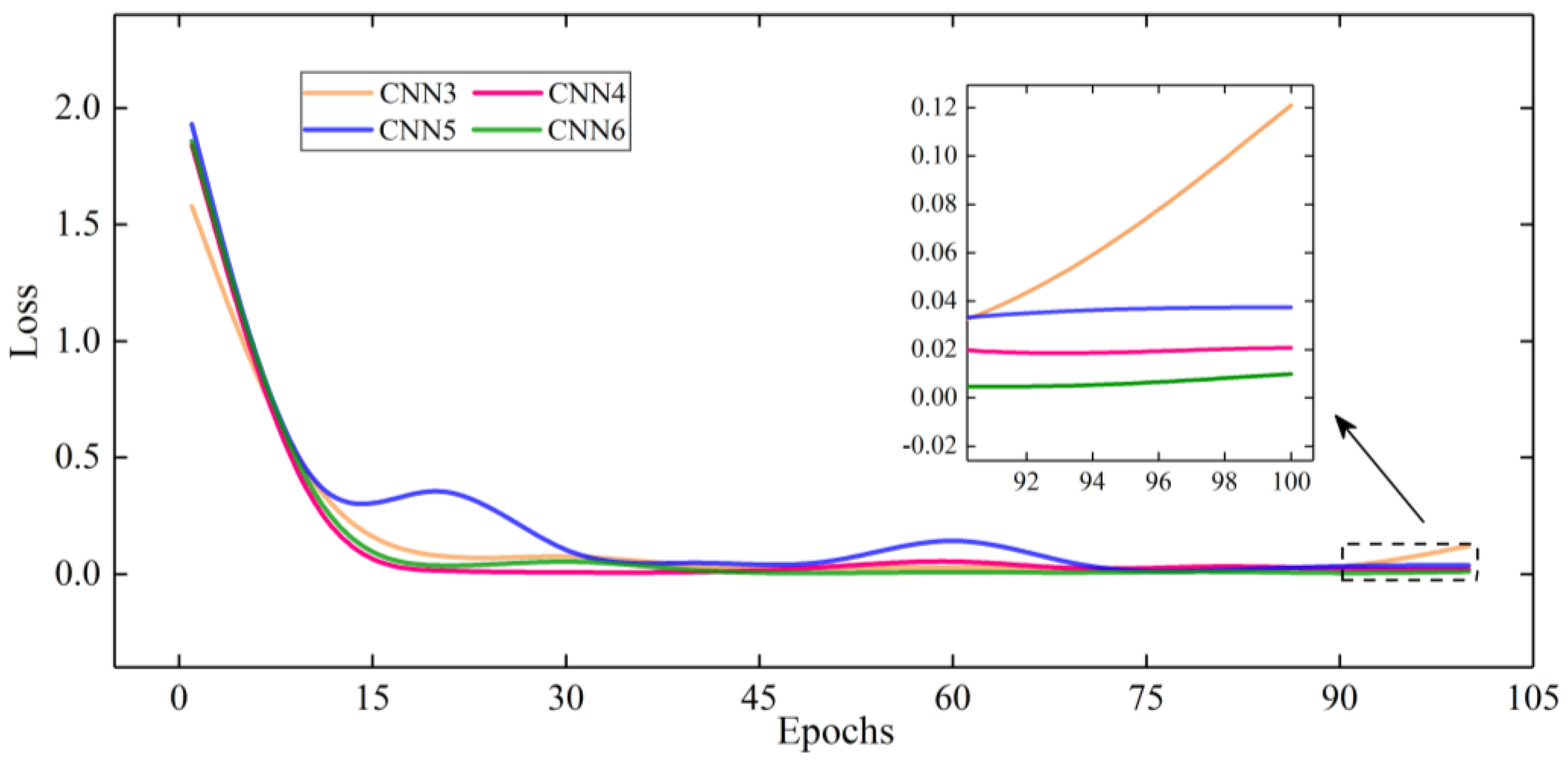
As discussed in Section 2, we found that the convolutional layer was the main building block of the HLCNN model. Three parameters affected the structure of the convolutional layer: convolutional kernel size, feature maps, and neurons. Here, the convolution kernel was able to achieve the feature extraction of the input sample. The feature map refers to the number of convolution kernels. In this paper, the convolutional layer directly affected whether the prediction model could completely extract the feature information from the design and operation parameters of centrifugal pump. Therefore, the same sample set was used to train three (CNN3), four (CNN4), five (CNN5), and six (CNN6) convolution layers to determine the influence of the convolutional layers on the HLCNN model. The simulation environment was a MATLAB 2020a with a 2.3 GHz CPU and 16 GB RAM.

The variation trend of losses with different convolutional layers is shown in Figure 5. From the curve comparison, it can be found that, except for CNN5, the training process of the other three networks was similar. In terms of model stability, the loss fluctuation of CNN5 was the largest compared with the other three networks under the same training epoch. The fluctuation was most obvious when the training epochs were 20 and 60. Therefore, CNN5 was not suitable for predicting the performance of the centrifugal pump. At the same time, CNN3 did not reach the convergence state for the feature learning speed of the model when the training epoch was 100. Finally, we selected a network with four convolution layers (CNN4) to predict the head and efficiency of the centrifugal pump after taking the impact of the training time into consideration. The hyperparameters of the selected network are listed in

Table 3. Hyperparameters of the selected CNN4.

Network Layer	Type	Parameters
		Convolutional Kernel Size	Feature Maps	Neurons
Input	Input layer	-	-	14
Conv1	Convolutional layer	1 × 3	16	-
Conv2	Convolutional layer	1 × 3	24	-
Conv3	Convolutional layer	1 × 3	24	-
Conv4	Convolutional layer	1 × 3	16	-
FCL1	Fully connected layer	1 × 1	-	32
FCL2	Fully connected layer	1 × 1	-	12
FCL3	Fully connected layer	1 × 1	-	6
Output	Output layer	-	-	6

.

The loss variation in the CNN4 model in the training and validation processes is shown in Figure 6. The results show that the loss gradually decreases with the increase in the learning epoch, and finally keeps near zero. There was no fluctuation or overfitting in the whole feature learning process. It indicates that the CNN4 model has robustness and fitting ability, and it can be utilized in modeling analysis of centrifugal pump performance.

4.2. Performance Prediction for the Test Samples

We used 78 test samples to evaluate the prediction effect of the HLCNN model. The comparison curve between predicted and experimental values of head and efficiency is shown in Figure 7. It shows that the values predicted by the HLCNN model were consistent with the change trend of the experimental values, and the difference was insignificant.

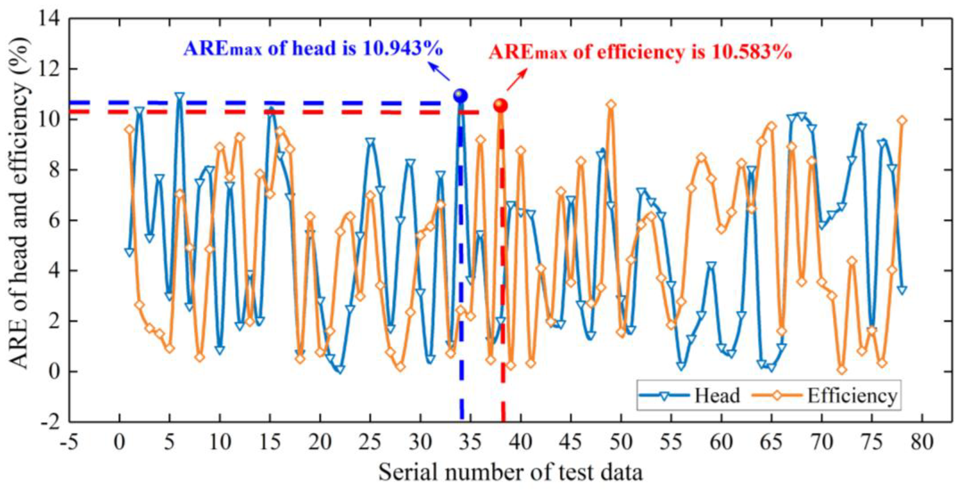
The ARE variations in the HLCNN model test samples are shown in Figure 8. It can be found that the ARE_means of the head and efficiency were both less than 9%, which meets the requirements of theoretical research and engineering practice [52]. The change in ARE indicates that it is feasible to use the HLCNN model to predict the energy performance of the centrifugal pump.

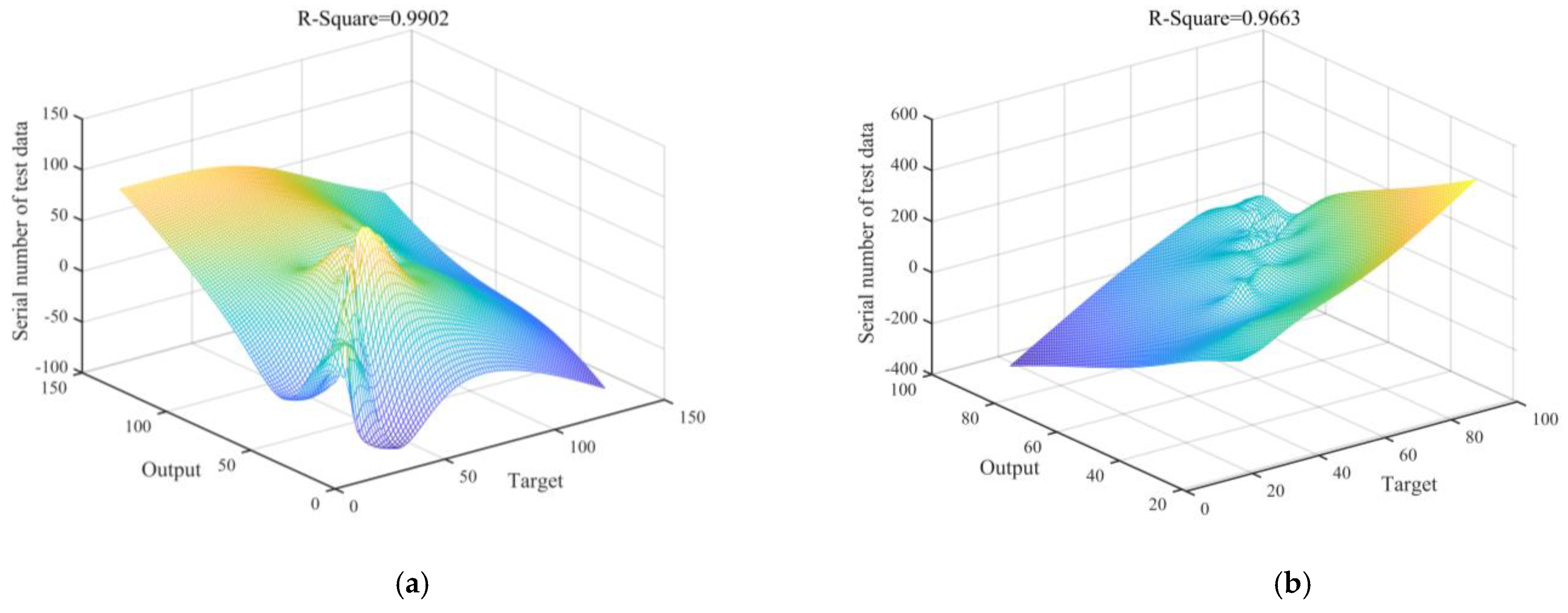
Once the head and efficiency predictions of the test samples are realized, Figure 9 can further illustrate the correlation between the prediction and the experimental results. It can be seen that the coefficients of determination (R−Square) of head and efficiency were 0.9902 and 0.9663, indicating that the HLCNN model has better fitting performance.

4.3. Comparison with the Other Machine Learning Models

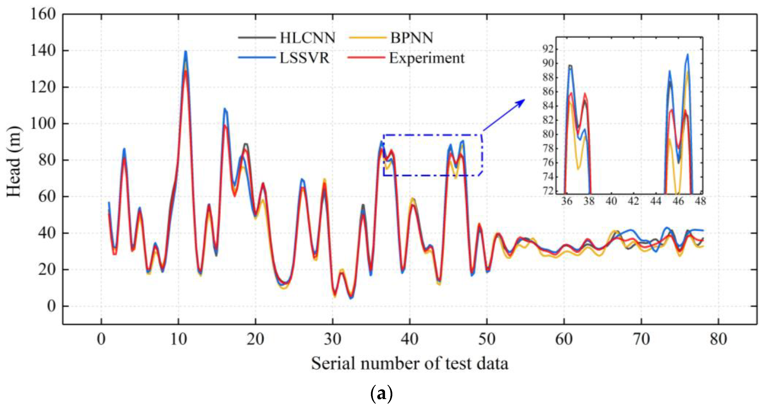
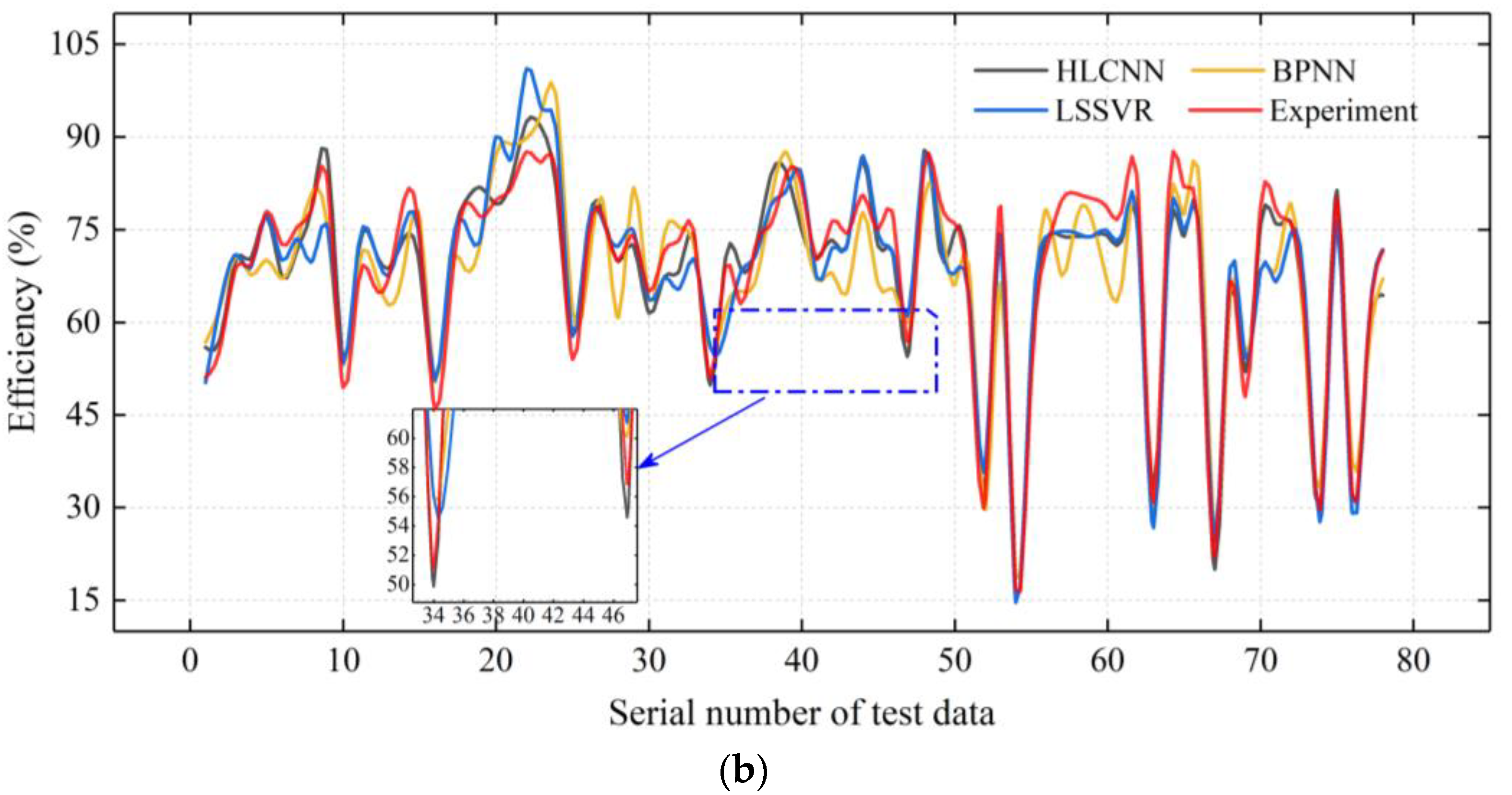
To further verify the nonlinear approximation ability of the proposed HLCNN model, we compared the prediction results of the HLCNN, the BPNN, and the LSSVR models. The same data set and running environment were adopted for the three models. The predicted results of the different models compared to the experimental results are shown in Figure 10. It can be seen that the fitting ability of the HLCNN model was better than that of the other two models in terms of predicting the head and efficiency of the centrifugal pump (as marked with the blue rectangles). This indicates that the problems of training process difficulties and model instability are solved by the HLCNN model compared with the traditional machine learning models.

Table 4. Comparison of evaluation indicators of different models on centrifugal pump head.

Model	AREmax	AREmin	AREmean	RMSE	SSE	MAE
HLCNN	10.943%	0.112%	4.866%	2.774 m	600.331 m2	0.783 m
BPNN	20.268%	0.252%	7.587%	3.607 m	1014.695 m2	1.053 m
LSSVR	15.318%	0.118%	5.718%	3.608 m	1015.125 m2	0.980 m

and

Table 5. Comparison of evaluation indicators of different models on centrifugal pump efficiency.

Model	AREmax	AREmin	AREmean	RMSE	SSE	MAE
HLCNN	10.583%	0.072%	4.769%	4.011%	0.125	0.443%
BPNN	16.724%	2.319%	8.019%	6.263%	0.306	1.217%
LSSVR	16.693%	0.316%	6.538%	5.154%	0.207	0.463%

summarize the error distributions of the different models regarding head and efficiency, respectively. It can be seen that the HLCNN prediction model obtained better ARE_max, ARE_min, ARE_mean, RMSE, SSE, and MAE values than the BPNN and LSSVR models. This indicates that the predicted head and efficiency of the HLCNN model and the experimental values have a great agreement, which means that it is more suitable for approximating the nonlinear mapping relationship between design, operation parameters, and energy performance of the centrifugal pump. At the same time, it is worth noting that the HLCNN model reduces the complexity of the prediction model with its special structure of local weight sharing, which is embodied in the data reconstruction in the process of centrifugal pump feature extraction.

4.4. Comparison with the CFD Method

According to many previous studies, the CFD method, which analyzes the relationship between the internal flow field characteristics and the external performance parameters, is another way to predict the performance of centrifugal pumps. In order to verify the prediction ability of the HLCNN model, the CFD flow field numerical simulation method was compared in this section. The simulation environment of the CFD method was the same as that of the MATLAB.

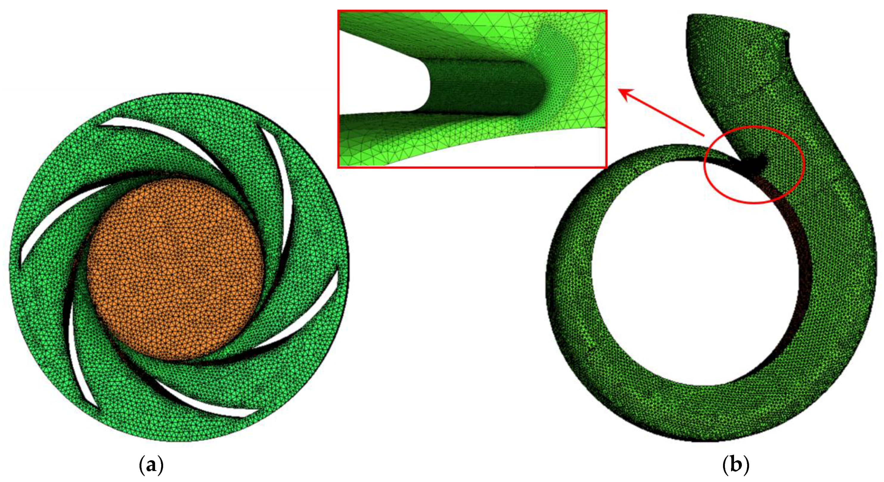
In this section, a centrifugal pump was selected randomly to reflect the variation in performance parameters with the flow rate. The design and operation parameters of the centrifugal pump are given in

Table 6. Design and operation parameters of impeller and volute of centrifugal pump.

Parameter	Value	Parameter	Value
Dj (mm)	76	D3 (mm)	15
D2 (mm)	137	b3 (mm)	30
b2 (mm)	14	φ0 (°)	22
z	6	Ft (mm2)	1477
β2 (°)	30	ns	129
dh (mm)	0	Qd (m3/h)	50
β1 (°)	17	n (r/min)	2900

. The impeller and volute, as two important components of the centrifugal pump, were divided into grids as shown in Figure 11.

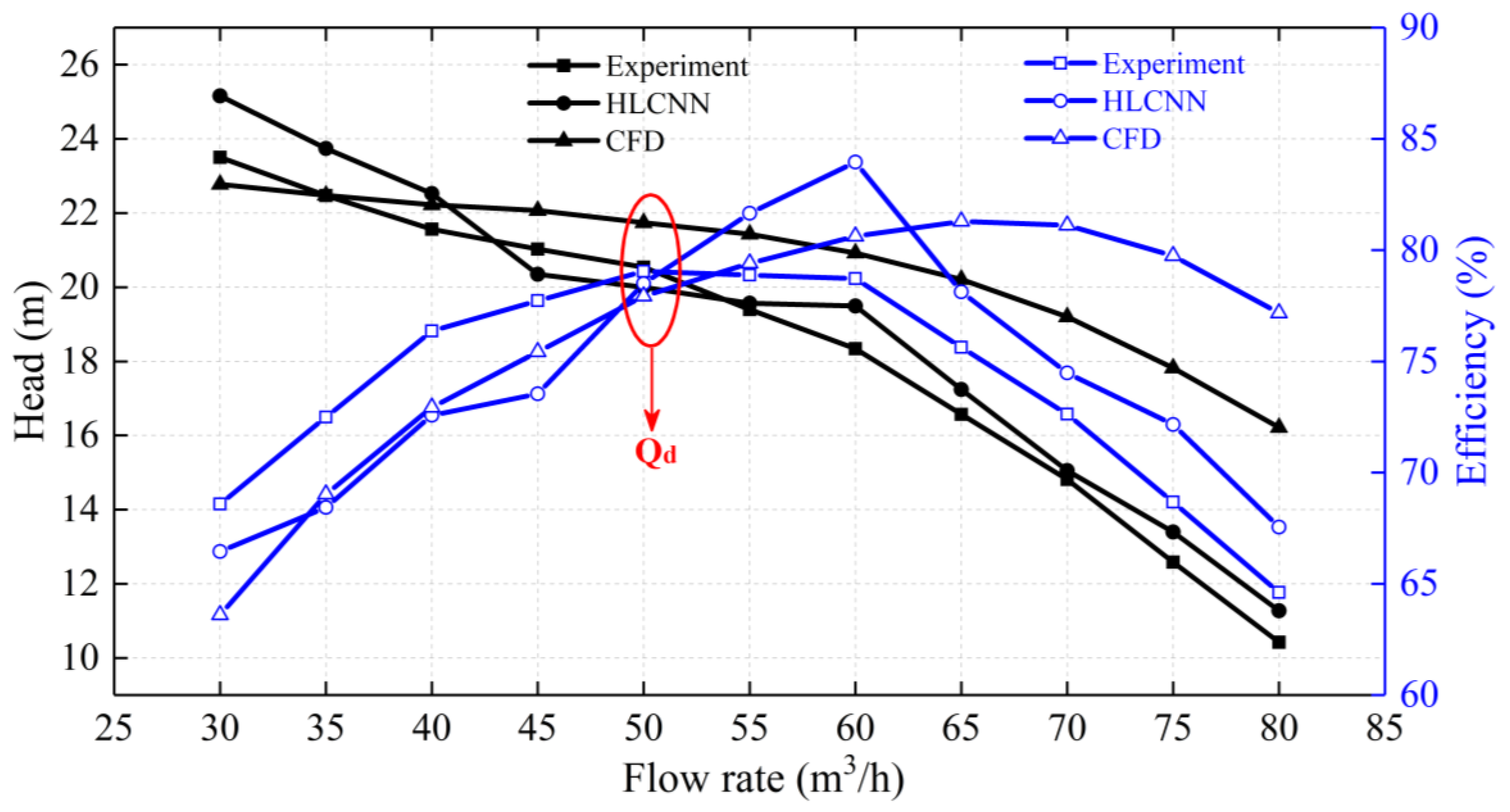
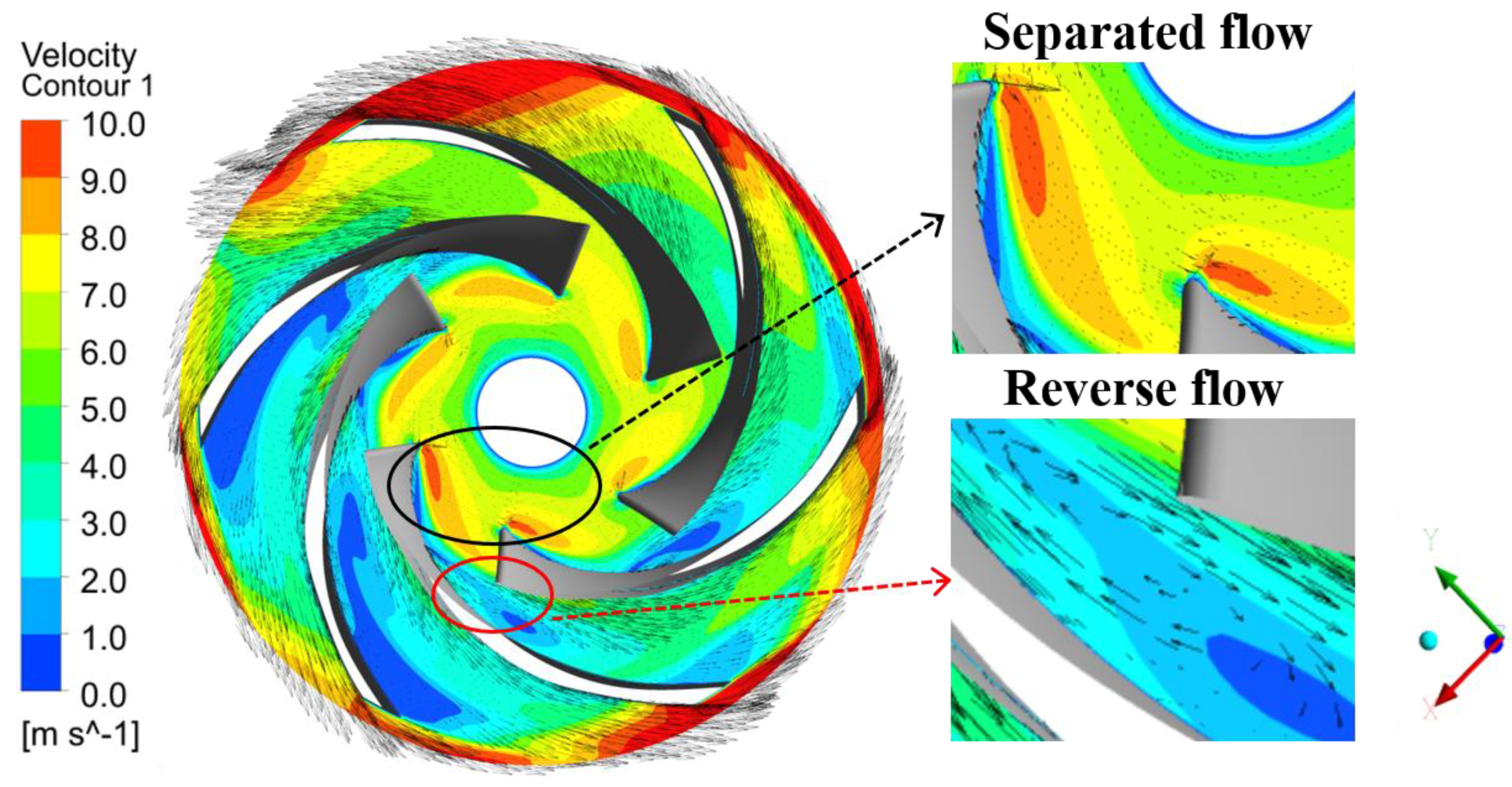
The changes in performance parameters of the centrifugal pump are presented in Figure 12. The research in Figure 12 shows that when the centrifugal pump was operating under design conditions (as marked with the green circles), the predicted values of the two models were both close to the experimental values, and those the HLCNN model proposed are particularly obvious. The predicted values of the CFD model gradually deviated from the experimental values when it operated in off−design conditions. There may be three reasons for this phenomenon: (1) The accuracy of the CFD method is limited by the influence of computer performance and engineer experience. (2) The inside flow pattern of the centrifugal pump has a high turbulence value. At the same time, the numerical simulation process is affected by turbulence model selection, separated flow, reverse flow, and other factors under off−design conditions (see Figure 13). (3) At present, the research of the interaction between the impeller and volute is not deep enough.

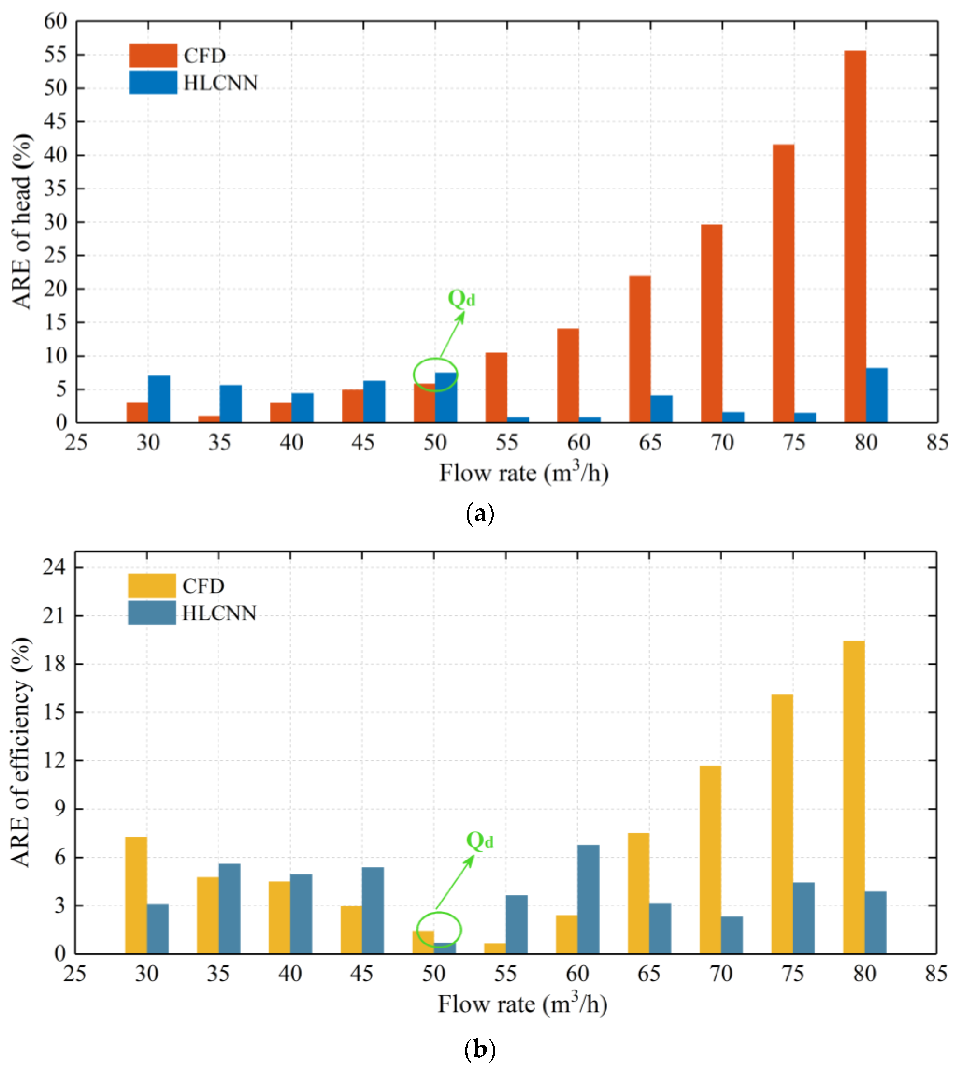
It can be found from Figure 14 that the ARE_means of the head and efficiency obtained by the CFD model were 17.30% and 7.16%. On the contrary, the ARE_means of the HLCNN model were 4.36% and 4.00%, respectively, proving the strong generalization ability of the HLCNN model within a wide flow rate range.

In addition, compared with the CFD method, the HLCNN model has advantages in the prediction time of centrifugal pump performance. The whole prediction process of the HLCNN model took 6.48 min in this section. However, under the same operating environment, the CFD method required 27.5 h to complete the performance predictions at 11 operating points (Q = 30~80 m³/h). Therefore, the HLCNN model built in this paper can build a CPPP model to meet the needs of design, production, and operation quickly and accurately.

5. Conclusions

This paper proposes a HLCNN-based method for predicting centrifugal pump energy performance. The results demonstrate that the HLCNN method can improve prediction accuracy compared with other methods. The following conclusions can be drawn:

(1) The performance features of the centrifugal pump were extracted by the HLCNN model, and a nonlinear mathematical relationship was established between the hydraulic loss of the centrifugal pump and the design operating parameters.

(2) The influence of convolution layers on the HLCNN model training process was analyzed, and it was determined that the network with four convolution layers (CNN4) was feasible to build the performance prediction model for the centrifugal pump.

(3) The HLCNN model prediction results were compared with the experimental results, and it was found that the ARE_means of head and efficiency were both less than 9%, which is consistent with the error range required by both theoretical research and engineering practice.

(4) The ARE_mean of the HLCNN model was lower in predicting the head and efficiency compared with the BPNN and the LSSVR model.

(5) The ARE_means of the HLCNN model were lower than the CFD method in predicting head and efficiency, and the whole prediction process only took 6.48 min. It indicates that the HLCNN model can predict the energy performance of centrifugal pumps in a wide flow rate range quickly and efficiently.

In light of the above analysis, the energy performance prediction method proposed in this paper only studies the centrifugal pump without considering more types of pumps, such as mixed-flow pumps, axial-flow pumps, etc. Hence, the first effort in future work should be to validate this idea. The second effort should be to analyze the internal flow mechanism on the basis of energy performance prediction combined with advanced flow field visualization technology, such as particle image velocimetry (PIV).

References

- Bing, H.; Cao, S. Multi-parameter optimization design, numerical simulation and performance test of mixed-flow pump impeller. Sci. China (Technol. Sci.) 2013, 56, 2194–2206. [Google Scholar] [CrossRef]
- Remo, J.; Carlson, M.; Pinter, N. Hydraulic and flood-loss modeling of levee, floodplain, and river management strategies, Middle Mississippi River, USA. Nat. Hazards 2012, 61, 551–575. [Google Scholar] [CrossRef]
- Wang, C.; Shi, W.; Wang, X.; Jiang, X.; Yang, Y.; Li, W.; Zhou, L. Optimal design of multistage centrifugal pump based on the combined energy loss model and computational fluid dynamics. Appl. Energy 2017, 187, 10–26. [Google Scholar] [CrossRef]
- Toti, A.; Vierendeels, J.; Belloni, F. Coupled system thermal-hydraulic/CFD analysis of a protected loss of flow transient in the MYRRHA reactor. Ann. Nucl. Energy 2018, 118, 199–211. [Google Scholar] [CrossRef]
- Qiu, C.; Huang, Q.; Pan, G.; Shi, Y.; Dong, X. Numerical simulation of hydrodynamic and cavitation performance of pumpjet propulsor with different tip clearances in oblique flow. Ocean Eng. 2020, 209, 107285. [Google Scholar] [CrossRef]
- Prakash, S.A.; Hariharan, C.; Arivazhagan, R.; Sheeja, R.; Raj, V.A.A.; Velraj, R. Review on numerical algorithms for melting and solidification studies and their implementation in general purpose computational fluid dynamic software—ScienceDirect. J. Energy Storage 2021, 36, 102341. [Google Scholar] [CrossRef]
- El-Ghafour, S.; Elghandour, M.; Mikhael, N.N. Three-Dimensional Computational Fluid Dynamics Simulation of Stirling Engine. Energy Convers. Manag. 2019, 180, 533–549. [Google Scholar] [CrossRef]
- Conti, F.; Wiedemann, L.; Sonnleitner, M.; Saidi, A.; Goldbrunner, M. Monitoring the mixing of an artificial model substrate in a scale-down laboratory digester. Renew. Energy 2018, 132, 351–362. [Google Scholar] [CrossRef]
- Motahar, S. Experimental study and ANN-based prediction of melting heat transfer in a uniform heat flux PCM enclosure. J. Energy Storage 2020, 30, 101535. [Google Scholar] [CrossRef]
- Tavakolpour-Saleh, A.R.; Shourangiz-Haghighi, A.R. A neural network-based scheme for predicting critical unmeasurable parameters of a free piston Stirling oscillator. Energy Convers. Manag. 2019, 196, 623–639. [Google Scholar]
- Nabipour, N.; Daneshfar, R.; Rezvanjou, O.; Mohammadi-Khanaposhtani, M.; Baghban, A.; Xiong, Q.; Li, L.K.; Habibzadeh, S.; Doranehgard, M.H. Estimating biofuel density via a soft computing approach based on intermolecular interactions. Renew. Energy 2020, 152, 1086–1098. [Google Scholar] [CrossRef]
- Zhang, J.; Wang, Y. Evaluating the bond strength of FRP-to-concrete composite joints using metaheuristic-optimized least-squares support vector regression. Neural Comput. Appl. 2020, 33, 3621–3635. [Google Scholar] [CrossRef]
- Lin, T.; Li, X.; Zhu, Z.; Xie, J.; Li, Y.; Yang, H. Application of enstrophy dissipation to analyze energy loss in a centrifugal pump as turbine. Renew. Energy 2021, 163, 41–55. [Google Scholar] [CrossRef]
- El-Naggar, M.A. A one-dimensional flow analysis for the prediction of centrifugal pump performance characteristics. Int. J. Rotating Mach. 2013, 12, 473512. [Google Scholar] [CrossRef]
- Li, W.G. Effects of viscosity on turbine mode performance and flow of a low specific speed centrifugal pump. Appl. Math. Model. 2016, 40, 904–926. [Google Scholar] [CrossRef]
- Shahverdi, K.; Loni, R.; Maestre, J.; Najafi, G. CFD numerical simulation of Archimedes screw turbine with power output analysis. Ocean Eng. 2021, 231, 108718. [Google Scholar] [CrossRef]
- Bhatti, M.; Arain, M.; Zeeshan, A.; Ellahi, R.; Doranehgard, M. Swimming of Gyrotactic Microorganism in MHD Williamson nanofluid flow between rotating circular plates embedded in porous medium: Application of thermal energy storage. J. Energy Storage 2022, 45, 103511. [Google Scholar] [CrossRef]
- Krzemianowski, Z.; Steller, J. High specific speed Francis turbine for small hydro purposes-design methodology based on solving the inverse problem in fluid mechanics and the cavitation test experience. Renew. Energy 2021, 169, 1210–1228. [Google Scholar] [CrossRef]
- Kang, C.; Mao, N.; Pan, C.; Zhu, Y.; Li, B. Effects of short blades on performance and inner flow characteristics of a low-specific-speed centrifugal pump. Proc. Inst. Mech. Eng. Part A J. Power Energy 2017, 231, 290–302. [Google Scholar] [CrossRef]
- Ur Rehman, A.; Shinde, S.; Singh, V.K.; Paul, A.R.; Jain, A.; Mishra, R. CFD based condition monitoring of centrifugal pumps. In Proceedings of the COMADEM 2013, Helsinki, Finland, 11–13 June 2013. [Google Scholar]
- Esfandiari, K.; Abdollahi, F.; Talebi, H.A. Adaptive control of uncertain Nonaffine nonlinear systems with input saturation using neural networks. IEEE Trans. Neural Netw. Learn. Syst. 2015, 26, 2311–2322. [Google Scholar] [CrossRef]
- Yu, L.; Dai, W.; Tang, L.; Wu, J. A hybrid grid-GA-based LSSVR learning paradigm for crude oil price forecasting. Neural Comput. Appl. 2016, 27, 2193–2215. [Google Scholar] [CrossRef]
- Mirabbasi, R.; Kisi, O.; Sanikhani, H.; Meshram, S.G. Monthly long-term rainfall estimation in Central India using M5Tree, MARS, LSSVR, ANN and GEP models. Neural Comput. Appl. 2019, 31, 6843–6862. [Google Scholar] [CrossRef]
- Zhao, B.; Ren, Y.; Gao, D.; Xu, L. Performance ratio prediction of photovoltaic pumping system based on grey clustering and second curvelet neural network. Energy 2019, 171, 360–371. [Google Scholar] [CrossRef]
- Mrinal, K.R.; Samad, A. Performance prediction of kinetic and screw pumps delivering slurry. Proc. Inst. Mech. Eng. Part A-J. Power Energy 2018, 232, 898–911. [Google Scholar] [CrossRef]
- Park, S.K.; Moon, H.J.; Min, K.C.; Hwang, C.; Kim, S. Application of a multiple linear regression and an artificial neural network model for the heating performance analysis and hourly prediction of a large-scale ground source heat pump system. Energy Build. 2018, 165, 206–215. [Google Scholar] [CrossRef]
- Nie, S.B.; Guan, X.F.; Liu, H.L. Exploration of using artificial neural network to predict the performance of centrifugal pumps. Pump Technol. 2002, 5, 16–18. [Google Scholar]
- Deng, H.; Liu, Y.; Li, P.; Zhang, S. Whole flow field performance prediction by impeller parameters of centrifugal pumps using support vector regression. Adv. Eng. Softw. 2017, 114, 258–267. [Google Scholar] [CrossRef]
- Zhang, Y.; Le, J.; Liao, X.; Zheng, F.; Li, Y. A novel combination forecasting model for wind power integrating least square support vector machine, deep belief network, singular spectrum analysis and locality-sensitive hashing. Energy 2019, 168, 558–572. [Google Scholar] [CrossRef]
- Krizhevsky, A.; Sutskever, I.; Hinton, G. ImageNet classification with deep convolutional neural networks. Adv. Neural Inf. Process. Syst. 2017, 60, 84–90. [Google Scholar] [CrossRef]
- Xie, C.; Kumar, A. Finger vein identification using convolutional neural network and supervised discrete hashing. Pattern Recognit. Lett. 2019, 119, 148–156. [Google Scholar] [CrossRef]
- Yang, N.; Song, Z.; Hofmann, H.; Sun, J. Robust State of Health estimation of lithium-ion batteries using Convolutional Neural Network and Random Forest. J. Energy Storage 2020, 48, 103857. [Google Scholar] [CrossRef]
- Pereira, J.; Saraiva, F. Convolutional neural network applied to detect electricity theft: A comparative study on unbalanced data handling techniques. Int. J. Electr. Power Energy Syst. 2021, 131, 107085. [Google Scholar] [CrossRef]
- Qi, C.R.; Su, H.; Nießner, M.; Dai, A.; Yan, M.; Guibas, L.J. Volumetric and multi-view CNNs for object classification on 3D data. In Proceedings of the IEEE Conference on Computer Vision and Pattern Recognition, Las Vegas, NV, USA, 27–30 June 2016; pp. 5648–5656. [Google Scholar]
- Kuo, C. Understanding convolutional neural networks with a mathematical model. J. Vis. Commun. Image Represent. 2016, 41, 406–413. [Google Scholar] [CrossRef]
- Ye, S.; Zhang, Z.; Song, X.; Wang, Y.; Chen, Y.; Huang, C. A flow feature detection method for modeling pressure distribution around a cylinder in non-uniform flows by using a convolutional neural network. Sci. Rep. 2020, 10, 4459. [Google Scholar] [CrossRef] [PubMed]
- Harbola, S.; Coors, V. One dimensional convolutional neural network architectures for wind prediction. Energy Convers. Manag. 2019, 195, 70–75. [Google Scholar] [CrossRef]
- Haidar, A.; Verma, B. Monthly rainfall forecasting using one-dimensional deep convolutional neural network. IEEE Access 2018, 6, 69053–69063. [Google Scholar] [CrossRef]
- Eom, Y.H.; Chung, Y.; Park, M.; Hong, S.B.; Kim, M.S. Deep learning-based prediction method on performance change of air source heat pump system under frosting conditions. Energy 2021, 228, 120542. [Google Scholar] [CrossRef]
- Díaz-Vico, D.; Torres–Barrán, A.; Omari, A.; Dorronsoro, J.R. Deep neural networks for wind and solar energy prediction. Neural Process. Lett. 2017, 46, 829–844. [Google Scholar] [CrossRef]
- Ma, Z.Q.; Zhang, S.C.; Ma, Y.; Deng, H.Y.; Zhang, Z.H.; Zhang, H.J. Non-overload optimization design of medium specific speed pump based on orthogonal design method. Fluid Mach. 2015, 43, 42–46. [Google Scholar]
- Zhang, Y.; Hu, S.; Wu, J.; Zhang, Y.; Chen, L. Multi-objective optimization of double suction centrifugal pump using Kriging metamodels. Adv. Eng. Softw. 2014, 74, 16–26. [Google Scholar] [CrossRef]
- Jain, S.V.; Swarnkar, A.; Motwani, K.H.; Patel, R.N. Effects of impeller diameter and rotational speed on performance of pump running in turbine mode. Energy Convers. Manag. 2015, 89, 808–824. [Google Scholar] [CrossRef]
- Hickman. Centrifugal Pump Design. Hrvatska Znanstvena Bibliografija i MZOS-Svibor. 2007. Available online: https://www.researchgate.net/publication/255096967_Centrifugal_pump_design (accessed on 16 May 2023).
- Gülich, J.F. Centrifugal Pumps; Springer: Berlin, Germany, 2014. [Google Scholar]
- Kim, K.H. Experimental Investigation under Water Condition on the Loss of Pipe Material Caused by Solid Particle Erosion in the Pipe Flow. Int. J. Fluid Mach. Syst. 2018, 11, 424–431. [Google Scholar] [CrossRef]
- Lei, C.; Yiyang, Z.; Zhengwei, W.; Yexiang, X.; Ruixiang, L. Effect of Axial Clearance on the Efficiency of a Shrouded Centrifugal Pump. J. Fluids Eng. 2015, 137, 071101. [Google Scholar] [CrossRef]
- Omar, A.K.; Khaldi, A.; Ladouani, A. Prediction of centrifugal pump performance using energy loss analysis. Aust. J. Mech. Eng. 2017, 15, 210–221. [Google Scholar] [CrossRef]
- Bhusal, N.; Kamruzzaman, M.; Benidris, M. A convolutional neural network-based approach to composite power system reliability evaluation. Int. J. Electr. Power Energy Syst. 2021, 135, 107468. [Google Scholar]
- Wang, H.; Zhou, J.; Liu, W.; Li, J.; Huang, X.; Liu, L.; Liang, W.; Yu, C.; Li, F.; Li, Z. BGD-based Adam algorithm for time-domain equalizer in PAM-based optical interconnects. Opt. Lett. 2020, 45, 141–144. [Google Scholar] [CrossRef]
- Atsalakis, G.S.; Valavanis, K.P. Surveying stock market forecasting techniques—Part II: Soft computing methods. Expert Syst. Appl. 2009, 36, 5932–5941. [Google Scholar] [CrossRef]
- Guan, X.F. Modern Pump Technology Manual; China Astronautic Publishing House: Beijing, China, 1995; pp. 746–751. [Google Scholar]
- Dixon, S.; Larry, H.C. Fluid Mechanics and Thermodynamics of Turbomachinery; Butterworth-Heinemann: Burlington, VT, USA, 2013. [Google Scholar]
Figure 1.
Main design parameters of a centrifugal pump. (a) Impeller. (b) Volute.
Figure 2.
HLCNN architecture of centrifugal pump hydraulic loss prediction.
Figure 3.
The flow chart of the HLCNN model framework.
Figure 4.
Centrifugal pump energy performance test rig. (1) Motor. (2) Centrifugal pump. (3) Suction sump. (4) Electric valve. (5) Pressure sensor. (6) Electromagnetic flowmeter. (7) Photoelectric sensor. (8) Data acquisition system.
Figure 5.
Loss variations in different convolution layers.
Figure 6.
The loss variation in the CNN4 in the training and validation processes.
Figure 7.
Prediction results of the HLCNN model test samples. (a) Head. (b) Efficiency.
Figure 8.
ARE variations in the HLCNN model test samples.
Figure 9.
Linear regression analysis of test samples. (a) Head. (b) Efficiency.
Figure 10.
Comparison of performance prediction of centrifugal pump with different models. (a) Head. (b) Efficiency.
Figure 11.
Grid meshing of a centrifugal pump. (a) Impeller. (b) Volute.
Figure 12.
Comparisons of the performance parameters obtained by the HLCNN and CFD models.
Figure 13.
Flow field structure in the centrifugal pump under off−design conditions.
Figure 14.
Comparisons of the AREs obtained by the HLCNN and CFD models. (a) Head. (b) Efficiency.