
Oil Discharge Trajectory Simulation at Selected Baltic Sea Waterway under Variability of Hydro-Meteorological Conditions

Department of Mathematics, Gdynia Maritime University, Morska St. 81-87, 81-225 Gdynia, Poland
Water 2023, 15(10), 1957; https://doi.org/10.3390/w15101957
Submission received: 7 March 2023
/
Revised: 17 May 2023
/
Accepted: 18 May 2023
/
Published: 22 May 2023
(This article belongs to the Special Issue Seas under Anthropopressure)
Abstract
:The paper deals with an important issue related to the identification, modelling, and prediction of environmental pollution in aquatic ecosystems of the Baltic Sea caused by anthropopressure. Water ecosystems are in danger nowadays because of the negative influence of chemical releases in seas, oceans, or inland waters. The crucial issue is to prevent the oil spills and mitigate their consequences. Thus, there is a need for methods capable of reducing the water pollution and enhancing the effectiveness of port and marine environment preservation. The challenge in implementing actions to remove and prevent horizontal oil discharge lies in accurately determining its shape and direction of oil spreading. The author employed a self-designed software utilizing modified and developed mathematical probabilistic models to forecast the movement and dispersion of an oil spill in diverse hydrological and meteorological conditions. This involved determining the trajectory and movement of a spill domain, which consists of elliptical sub-domains undergoing temporal changes. The research results obtained are the initial results in the oil spill simulation problem. This approach represents an expanded and innovative method for determining the spill domain and tracking its movement, applicable to oceans and seas worldwide. It expands upon the methodologies firstly discussed, thereby broadening the range of available techniques in this field. A simple model of an oil spill trajectory simulation and a surface oil slick as an ellipse is illustrated using a time-series of selected hydro-meteorological factors that change at random times. The author proposes a Monte Carlo simulation method to determine the extent of an oil spill in an aquatic ecosystem, taking into account the influence of varying hydro-meteorological conditions. A semi-Markov model is defined to capture the dynamics of these conditions within the spill area and develop an enhanced algorithm for predicting changes in the shape and movement of the spill domain under changing these conditions. By applying the algorithm, a simulation is conducted to provide short-term prediction of the oil discharge trajectory in a selected Baltic Sea waterway. To enhance the accuracy of predicting the process of changing conditions, uniformly tested joint datasets from the open sea water area were incorporated. Finally, the potential future prospects and directions for further research in this field are discussed.
1. Introduction
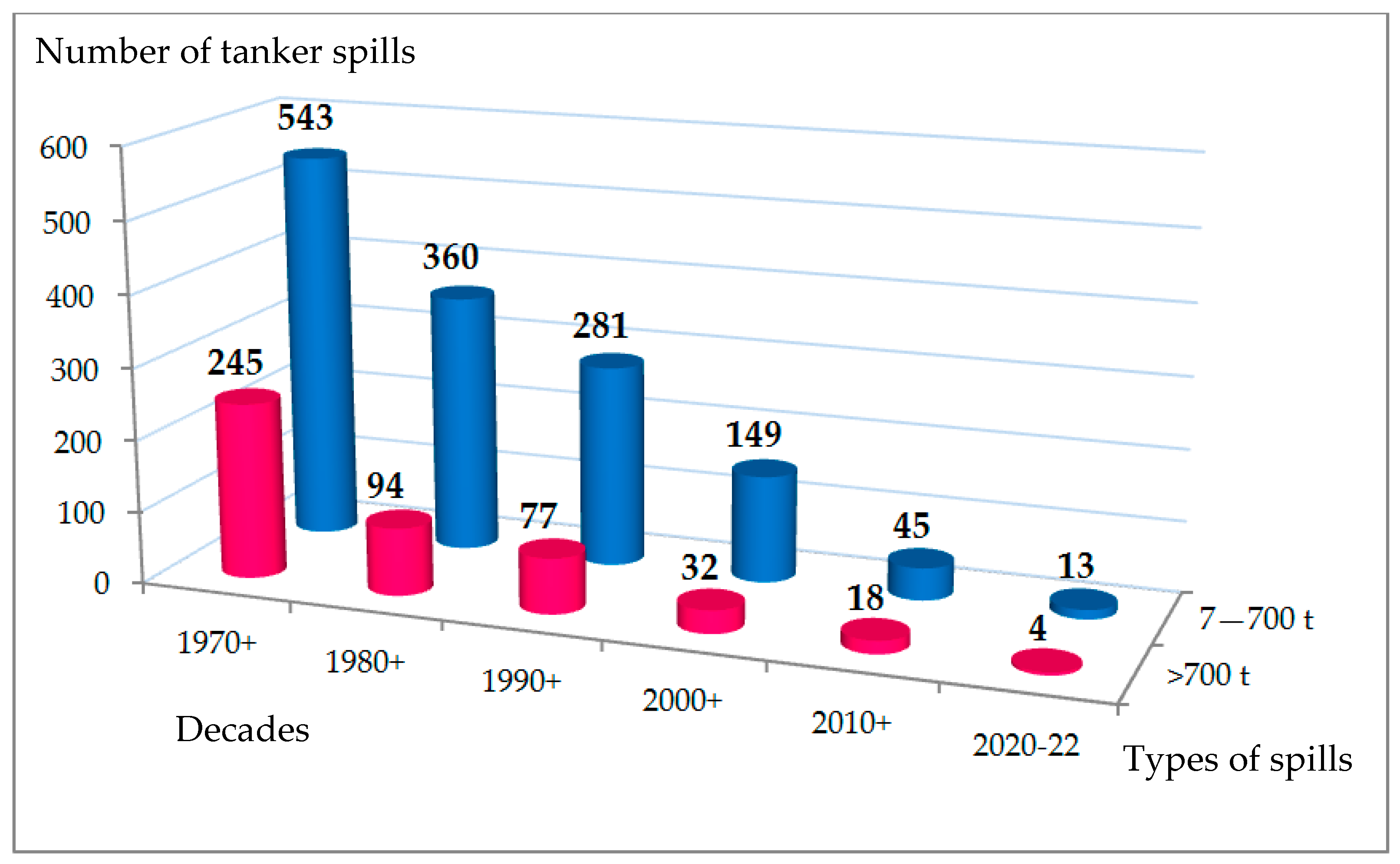
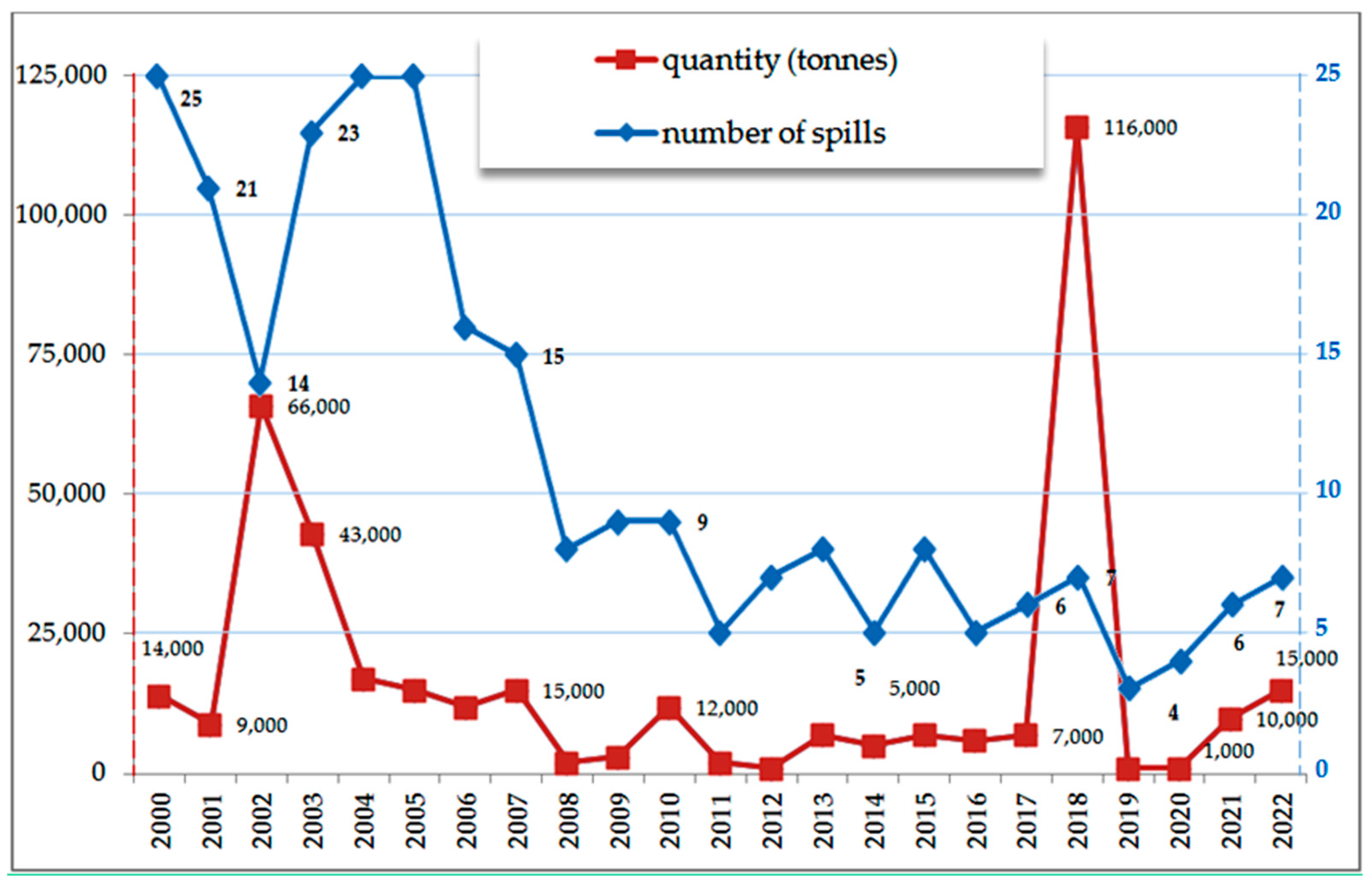
In recent years, a large threat of chemical releases into international waters has been observed. This pollution means that the concentration of toxic substances is harmful to the environment and local economy [1,2], which implies that the effects can harm biological life and affect human activities. Any intentional or accidental action that results in the spill, emptying, dumping, pumping, emitting, or pouring of oil into water is considered a discharge of oil [3]. The main causes of pollution are seabed exploration and drilling platform construction, oil transport by ships and pipelines, pollution during drilling and pipelines operation, contamination from rivers, and illegal oil discharges from ships [4]. There were four medium spills (7–700 tonnes) and three large spills (>700 tonnes, in Asia and Africa) in 2022 with total volume of around 15,000 tonnes [5]. The current trends seem to be downward, however some fluctuations still occur (Figure 1 and Figure 2).
The significant issue is to forestall the oil slicks and mitigate their cost to the nations and wildlife affected. The oil spill on the water surface behaves very differently depending on its chemical composition as well as on the hydrological parameters of the basin [1]. The removal of pollution, especially oil discharge in the open sea area, is very difficult due to the variability of hydro-meteorological conditions [1,2]. The spreading of oil generally depends on wind, wave height, and currents [1,6].
In terms of transport intensification, the Baltic Sea is widely recognized as one of the most congested seas globally. In the era of globalization of the economy, we can observe a negative impact of chemical releases, especially during winter, when the sun light falls on the Earth with less intensity and the days are shorter [7,8,9,10]. In terms of threats to the Baltic Sea, maritime transport is one of the most dangerous factors affecting the environment. That is why safety issues should be considered, especially in the Baltic Proper basin [1]. Difficulties associated with reaching the scene of the event, carrying out the action, the risk of sinking the ship, including fuel sunk and large amounts of dangerous cargo on board, cause disasters on a scale of much larger areas compared to disasters on land [1]. Due to the amount of transported cargo, the greatest threats of an ecological disaster as a result of accidents come from oil tankers and container ships. It will certainly not be indifferent to the flora and fauna of the sea, and thus to other sea users. There is also the fear that the effects of contamination will be felt for a long time after the accident occurred.
This research problem of sea pollution identification, modelling, and prediction due to the spills of hazardous substances has existed for many years and is becoming more and more significant due to the intensive development of marine water purity monitoring systems [5,6,7,8,9]. The increase in computerization, automation, and miniaturization of measurement and navigation systems leads to the prevention and quick detection of oil spills by means of monitoring activities, including those from space and SAR (search and rescue) radars [10,11,12,13,14,15,16]. However, these data are often unavailable for the specified time period, and thus numerical models and cutting-edge monitoring methods must be integrated. Moreover, in [1], it is stated that even the satellite-based systems can have a lot of false and missing detections. Out of the almost 800 synthetic aperture radar (SAR) images of spills observed in the Baltic Sea, approximately 94% were classified as having medium or low confidence levels. In contrast, only approximately 45% of the almost 70 confirmed incidents of oil pollution in the Latvian Baltic region were detected by SAR. Additionally, around 40% of the SAR detections corresponded to slicks or minor quantities of oil. By appropriately selecting a model that considers the influence of changing hydro-meteorological conditions on the movement and dispersion of pollution spots, relevant authorities can effectively respond with timely rescue actions in real-time. Such a model would enable accurate predictions and monitoring of the spread of pollutants, allowing for proactive measures to mitigate the impact on the environment and ensure swift response and containment efforts [2,9,11,15,17,18,19].
There are many methods allowing for the determination of the oil spill area, marking the domain, and predicting its trajectory to prevent ecological disasters. Their level of complexity, ease of use, and applicability vary depending on what features are most reasonable in a given sea basin. The big marine disasters concerned with oil spill [20] made the scientific community interested in this topic, and this resulted in the appearance of a large number of models [16,21,22,23]. According to the TAC (Technical Advisory Committee) on oil spill prevention and response it is possible to determine two categories of oil spill response [16,22,23,24]. Oil weathering models evaluate the changes over time without predicting the expected drift direction. The common approaches proposed in the literature, including the hydro-meteorological impacts, are often based on the historical statistical data, which is a reasonable approach. In the second group, there can be found models, such as: deterministic trajectory models, hind cast, stochastic models, and three-dimensional models (longitude, latitude, depth), which predict the oil behaviour and spread over time. Nevertheless, the chemical properties of oil were initially skipped [25] and later considered [26]. National Oceanic and Atmospheric Administration—NOAA provided a report, also including hazmat mapping as a third oil spill modelling tool [24]. A substantial amount of literature and numerous existing models have been developed to describe the movement of oil on the water surface, employing varying degrees of physics-based approaches. Examples of commonly utilized models include OpenDrift, SpillCalc, OSCAR, Mike, and SIMAP [1]. These models have been extensively studied and documented, providing valuable insights into understanding and predicting the behaviour of oil discharges in marine environments. The mathematical models and stochastic simulation software, such as GNOME, PISCES II, MEDSLINK-II, POSEIDON, STW, MOTHY, DieCAST-SSBOM, and COZOIL, can be used to mitigate the consequences of oil spills [6]. Several investigations have been performed on this topic [27,28,29,30,31,32,33,34,35]. Not all the studies are considered in the references because the research topic is extensive, but they are mostly based on ready-made models, instead of proposing the original ones from scratch.
An important issue in the implementation of the action of removing and stopping the spill is to determine precisely the shape and direction of oil spread [1,2,6,8,11,33,35,36,37]. To do this, author proposed their own written software based on modified and developed mathematical models [18,38,39,40] for predicting the horizontal spill movement and spreading in changing hydro-meteorological conditions through determining the oil spill domain composed of changing in time its surface elliptical sub-domains. Thus, the simple model of a surface oil slick as an ellipse is driven in the paper by a time-series of selected hydro-meteorological factors that change at random times. The algorithm developed for predicting oil spill trajectories and investigating the movement of domains is applicable universally, as it can be utilized in various areas of the Baltic Sea that share similar conditions related to hydrology and meteorology. This universality can be achieved through scientific experimentation and statistical identification of the model’s required parameters. By employing a simulation-based approach, real-time information can be provided to oil spill responders, enabling them to take prompt and informed actions. The research results obtained are the initial results. The model can be developed to provide a helpful reflection of reality with greater precision.
2. Process of Changing Hydro-Meteorological Conditions
2.1. Definition
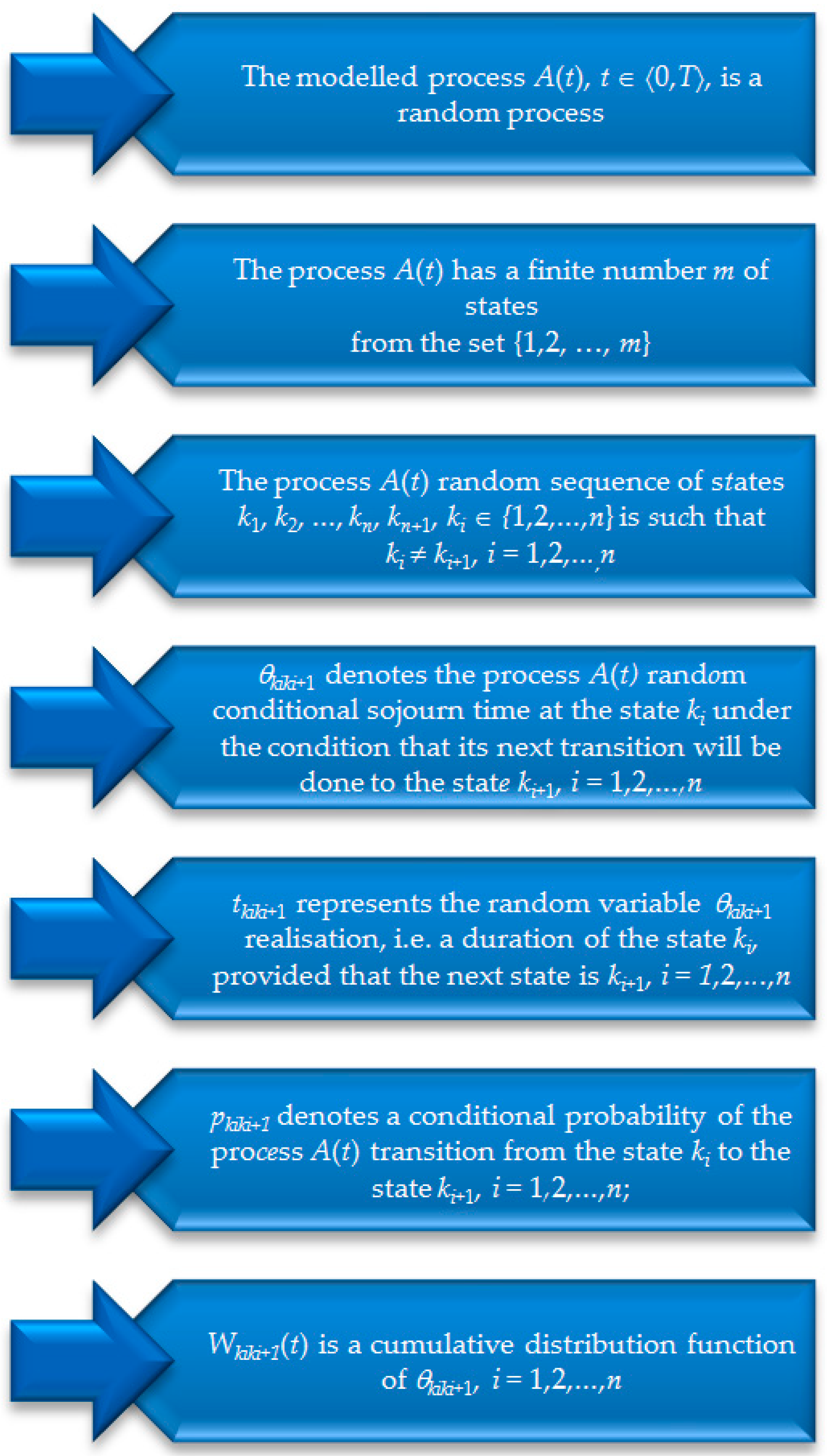
Using the semi-Markov model [41,42], to mathematically model the process A(t), t ∈ 〈0, T〉, of varying hydro-meteorological (h-m) conditions during time T, T > 0, the necessary assumptions and denotations are presented in Figure 3 [43,44,45,46].
The paper considers the semi-Markov approach as a more flexible and adaptable alternative to the conventional Markov model. Unlike the Markov model, which assumes exponential distributions for conditional sojourn times in specific h-m states, the semi-Markov approach allows for non-exponential distributions. This means that the model can accommodate any distribution of sojourn times in the respective states, providing a more realistic and accurate representation of the process. As a result, the semi-Markov approach is considered more practical, offering a better depiction of the real-world conditions.
In the following Section 2.2 and Section 2.3, the parameters for selected Baltic Sea waterway area are identified and the input data for Monte Carlo simulation are presented, assuming the initial time t = 0 (starting point). Once statistical data are collected, such as the number of initial states, counts of transitions between the states, and realizations of conditional sojourn times, the next step is to identify statistical parameters. This involves calculating the related probabilities and verifying the hypotheses regarding the distribution functions of the considered variables.
2.2. Parameters Identification for Selected Baltic Sea Waterway Area
Following a maritime accident and the subsequent release of oil, the resulting oil slick disperses and spreads across the water surface [7,20,22,26,35,47,48,49]. This happens due to gravity and interfacial tension [1,26,33,35,39]. The gravity influence decreases with time, but nevertheless the oil is still spreading [50]. Moreover, the hydro-meteorological conditions often significantly accelerate and lengthen the oil spread on the surface dependently on the wind direction and the wave height [1,23,26,33,49,51,52], especially in the open sea area. After consulting with experts from the polish Institute of Meteorology and Water Management, National Research Institute—IMWM-NRI, certain h-m factors were identified as having a significant impact on the trajectory of spill in the Baltic Sea waterway area. These selected factors were considered essential for understanding and accurately predicting the behaviour of the spills in that specific region:
- the velocity and direction of the wind;
- the height of the sea water level and waves;
- the direction of the currents;
- any obstacles to visibility such as fog or icing.
Therefore, we are engaged in studying the impact of these certain parameters on the shape and horizontal movement of the oil spill. We distinguish m = 6 states from {1, 2, …, 6} of the process of changing h-m conditions A(t), where t ∈ 〈0, T〉 [40,42] for the selected Baltic Sea open waters area defined by two parameters, the wave height (wh) and the wind speed (ws), presented in Table 1.
Statistical methods are essential for determining the unknown parameters of the process to apply practically the simulation to the prediction of the oil discharge trajectory, considering the states of this process [40,42,53]. If the statistical data come from various experiments or the datasets are collected at different times but contain measurement points close to each other at the considered area, before the identification of parameters, the investigation of these data uniformity is necessary [42,54]. The uniformity testing procedure for the process of varying h-m conditions data, including realisation from different experiments or the datasets, is presented, e.g., in [42]. In the aforementioned work, the methods for estimating the probabilities of the initial process states (from Table 1), the probabilities of transitions between these states, and the distributions of the process’s sojourn times are discussed [17,18,40,41,42,44,45,46,47,48] and should be firstly applied.
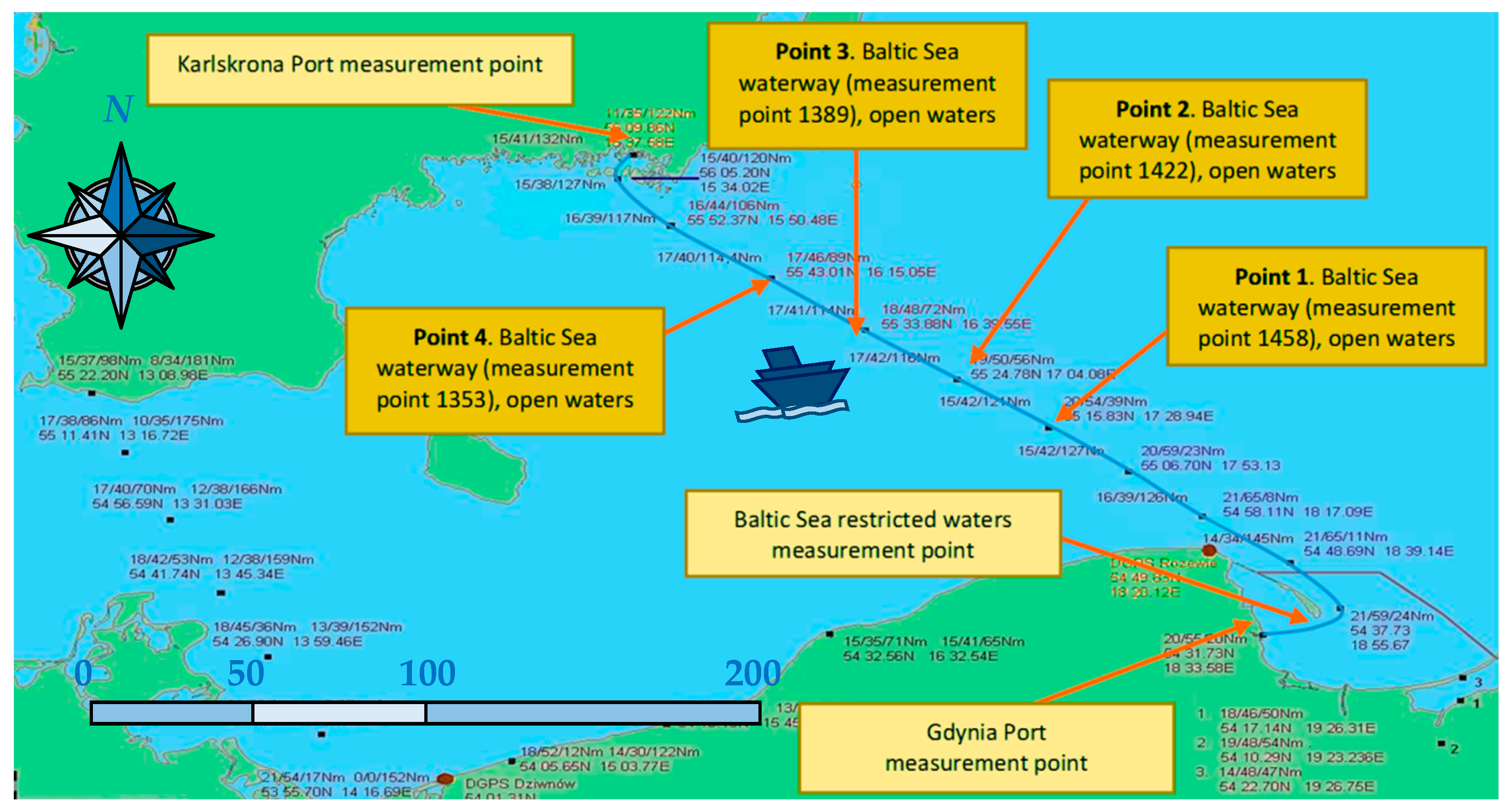
The study focuses on analyzing the variations in h-m conditions specifically in the selected Baltic Sea waterway within the open waters area (excluding ports area and restricted water area) presented in Figure 4. The blue line is a waterway of a passenger ro-ro ship sailing from Gdynia to Karlskrona. The four points are the measurement points given from IMWM-NRI. The approximate coordinates are given on the map, whereas the four different measurement points: 1353, 1389, 1422, and 1458, are marked precisely in cooperation with the Institute.
Datasets of statistical nature were gathered over a six-year period (Θ = 6), specifically during the month of March, at open waters area [56]. First of all, the IMWM-NRI prepared data, including wh and ws (see Table 1) at the selected measurement points (1–4), as shown in Figure 4. The interval was 3 h. Thus, each year there were approximately 365 × 8 = 2920 records saved. Multiplying this number accordingly by 6 years was sufficient to perform the analysis. It made sense to choose one month due to varying conditions in the Baltic Sea, e.g., in June there are different winds than in February and March. This month was selected because from January to March there are more accidents than in the summer months, which is closely related to the storms, temperature, humidity, and visibility that occur. During that period, the weather in Sweden undergoes rapid changes, ranging from strong winds and storms to calm breezes. This factor is of significant importance in the investigation. The data were obtained from the IMWM-NRI under a copyright provision such that they can be presented in a processed form, not the exact original. Following the uniformity testing, the data collected from the four points (as depicted in Figure 4) were combined and subjected to analysis using methods outlined in [40,41,42,57,58,59,60,61]. Based on this consolidated dataset, the unknown fundamental parameters of the semi-Markov model of the process at the selected water area were assessed and evaluated.
Every day at 3 am in March during the 6-year period, the wh and the ws were checked. Then, according to Table 1, the initial state of the process, from {1, 2, …, 6}, was assigned. After that, all the initial realizations ni, i = 1, 2, …, 6, were counted and presented in Table 2.
Next, there were calculated the initial probabilities of the considered h-m conditions:
p1(0) = 405/680 ≈ 0.595, p2(0) = 0.349, p3(0) = p4(0) = 0, p5(0) = 0.04, p6(0) = 0.016;
Further, all the possible transitions between the 6 states were calculated. Every 3 h (3:00, 6:00, 9:00, 12:00, 15:00, 18:00, 21:00, 24:00), an evaluation was performed to assess whether the process continued or changed its state, i.e., if the two considered parameters (wh and ws) remain the same as 3 h ago or their value changed noticeably. Table 3 illustrates the obtained results.
According to the above table, there were calculated the probabilities of transitions between the process’ states:
p12 = 1516/(1516 + 1 + 31) ≈ 0.98, p15 = 0.02, p21 = 0.7, p25 = 0.3, p32 = 0.92, p35 = 0.08, p45 = 1,
p52 = 0.76, p53 = 0.01, p56 = 0.23, p62 = 0.41, p63 = 0.15, p65 = 0.44.
p52 = 0.76, p53 = 0.01, p56 = 0.23, p62 = 0.41, p63 = 0.15, p65 = 0.44.
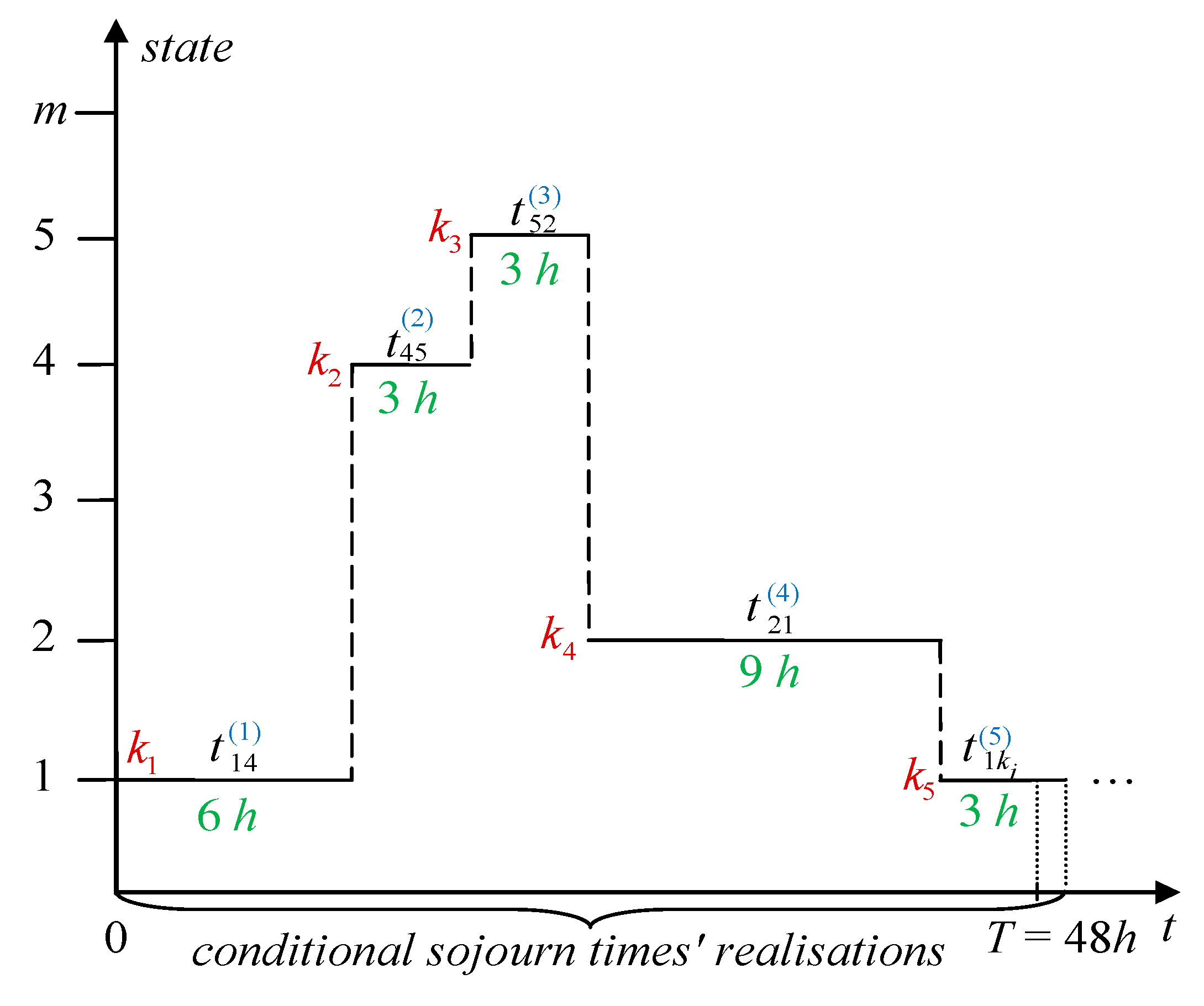
The process is analyzed with respect to changes in time states. According to Section 2.1, the symbol θkiki + 1 denotes the process’ random conditional sojourn time at the state ki under the condition that its next transition will be to the state ki + 1, i = 1, 2, …, n. For instance, the process is at the state k1 = 1 (wh up to 2 m and small ws up to 17 m/s), but under the condition it will go to the state k2 = 4 (the wave remains the same, but wind is changing). That change has happened once and the realisation time tk1k2 = t14 = 6 h. Next, we are at the state k2 = 4 and the next transition was to the state k3 = 5 (wave height increased up to 5 m plus there is a strong wind) and lasted for 3 h, which means tk2k3 = t45 = 3 h. An example of a process’s A(t) realization is presented in Figure 5.
Moreover, the hypotheses on the distribution functions Wkiki+1(t) were verified based on the sufficiently large realization number tkiki+1, and the empirical distribution functions were determined for the numbers of realizations less than 30.
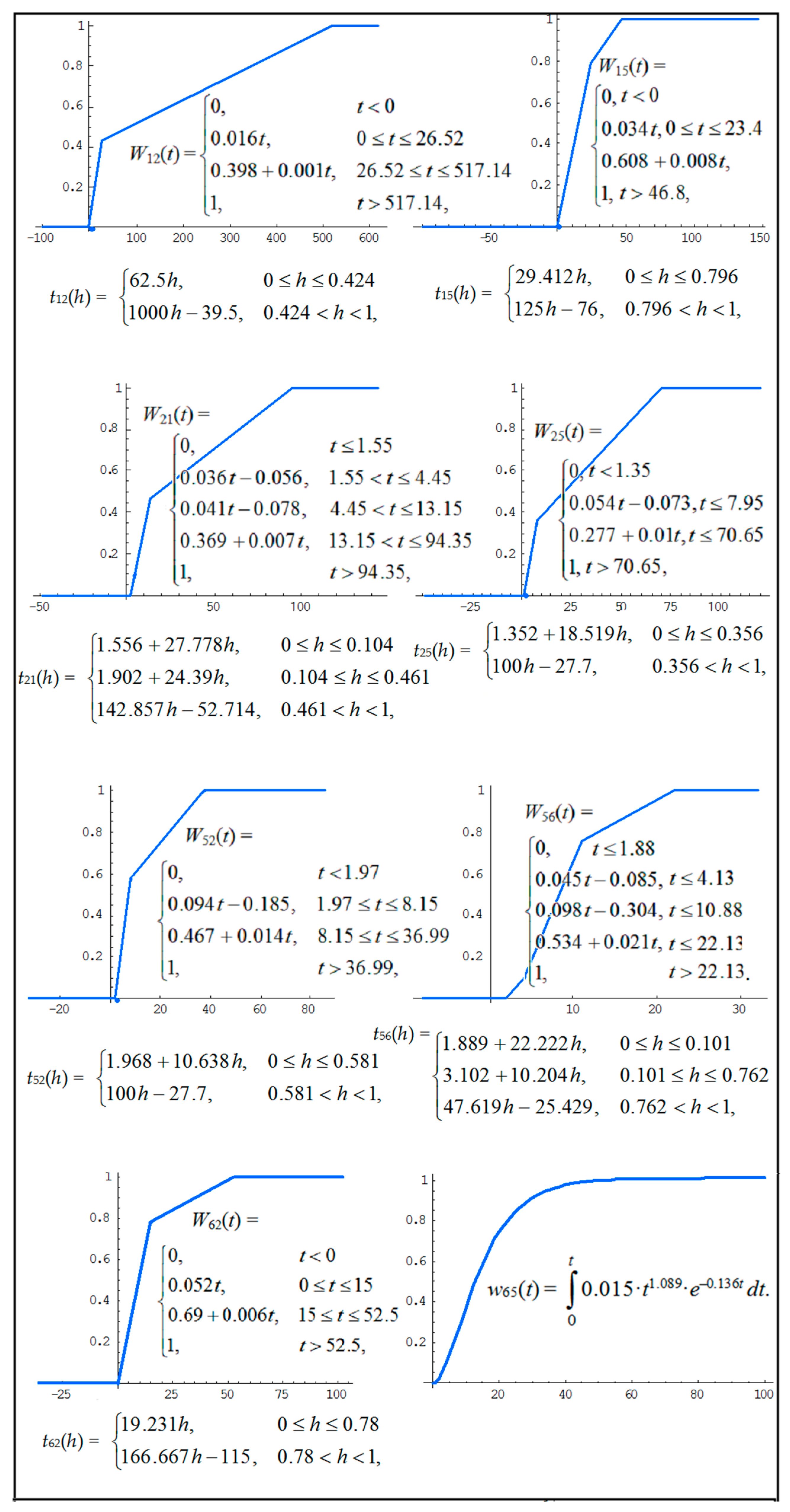
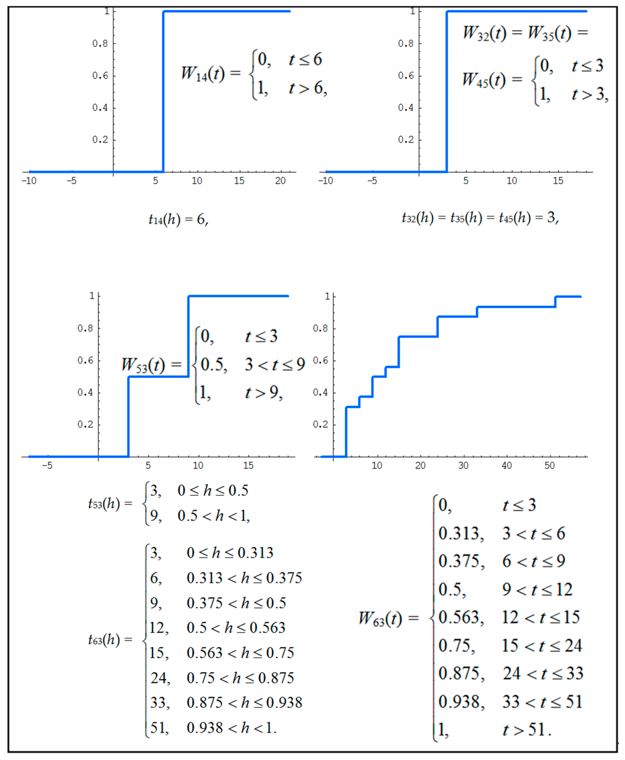
The collection of realizations of θkiki+1 representing the conditional sojourn times, where {ki, ki+1} = {{1,2}, {1,5}, {2,1}, {2,5}, {5,2}, {5,6}, {6,2}, {6,5}} were significantly large, and after verification it was confirmed that they exhibit chimney distributions (θ12, θ15, θ21, θ25, θ52, θ56, θ62) and gamma distribution (θ65), while the distribution functions of θ14, θ32, θ35, θ45, θ53, θ63 have the empirical distribution functions (Figure 6 and Figure 7). Formulae of the functions Wkiki + 1(t) are approximated to three decimal places, whereas in the graphs there are illustrated functions drawn without that approximation. The chimney distribution is introduced in a book [42], Chapter 2, page 58. This distribution got its name from chimneys because of the chimney look of the density function. The chimney distributions were used because they fit very well to the given data sets. However, a few distribution functions have the empirical distribution functions and none of the common distributions can fit well to the data (at least 30 distributions were checked with 1% to 10% critical interval). Moreover, some transitions to next states do not appear frequently and there were a few realisations. For instance, a transition between states 1 → 4: wh up to 2 m and small ws up to 17 m/s that increases above that value without much change in the wave height happened once during the considered period of time. Thus, empirical distributions were used.
The illustrated graphs and the presented formulae for distribution functions in Figure 6 and Figure 7 are later used in Section 2.3 to predict the h-m conditions using simulation method. There are multiple methods available for generating random samples from a specified probability distribution. Examples of such transform methods include the inverse method, the Box-Muller (B-M) method, and Marsaglia and Tsang’s rejection sampling (MTRS) method. This paper employs the inverse transform method for generating the realizations from . The gamma distribution realisations are generated using the MTRS method. The values are generated from transformation of the Gaussian function.
2.3. Input Data for Simulation
The data input to the simulation method based on the parameters identified in Section 2.2 are as follows:
- the experiment time T = 48 h;
- formula for generating the initial state coming from (1)
- formula for generating next states
constructed using (2), where g is a number that is randomly generated from the uniform distribution over the interval 〈0,1);
The experiment time is chosen as a short-term forecast, because the first two days of an oil discharge are of utmost importance to accurately determine the shape and direction of spread to implement quickly the action of removing the pollution. The simulation time can of course be increased, even by much. However, for long time prediction, another method should be used.
3. Algorithm
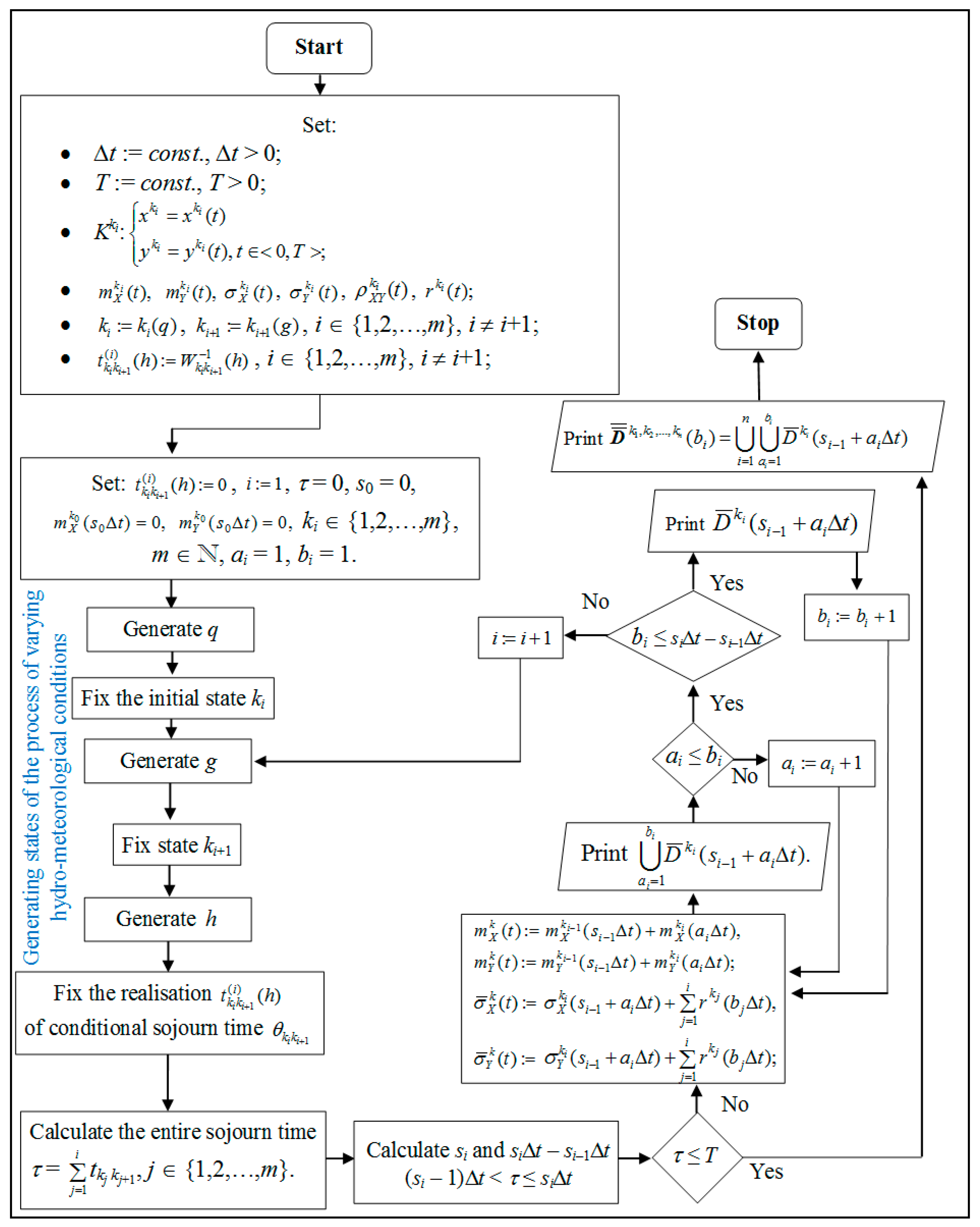
Figure 8 presents an expanded algorithm that proposes a method for determining the trajectory of oil discharge by taking into account its horizontal movement, which is influenced by varying h-m conditions. This is based on a probabilistic approach [17,18,40] and an extended approach from [39].
The process of varying h-m conditions at the selected water location where the oil spill occurred, depending on the specific incident being referred to, is constructed in the previous section. The h-m conditions presented in Table 1 are considered in the input model in Equations (3) and (4) which are generated from Equations (1) and (2) and equations derived from Figure 6 and Figure 7. Moreover, Equation (5) determines the parametric equations for the drift trend curve of the central point of the oil spill domain under different h-m conditions. These equations serve as the input for the model, allowing for the prediction of how oil drifts over time based on the specific conditions experienced.
The algorithm can consider more than two hydro-meteorological factors, e.g., wave height, wind speed, wind direction, ice conditions, sea water level, etc., and generates surface elliptical sub-domains, where actions of mitigation should be taken to reduce the pollution at the oil spill water area. In this paper, only two parameters were intentionally taken into consideration. For example, to add a third, fourth, or more parameters to Table 1, the data should be firstly grouped into sets and the table needed to be extended accordingly. For the purpose of this article, in order not to present (already) too many mathematical calculations, a simple example is illustrated in Section 4, to make the paper familiar to the reader.
This algorithm operates under the assumption that the oil spill central point at t, t ∈ 〈0, T〉, while the process of varying h-m is at the state ki, i = 1, 2, …, n, and has the normal distribution with the parameters that will be slightly modified [39,40]:
- expected values
- standard deviations , ;
- correlation coefficient .
Moreover, it is assumed that the oil spill domain radius at ki, i = 1, 2, …, n, is dependent on time t ∈ 〈0,T〉.
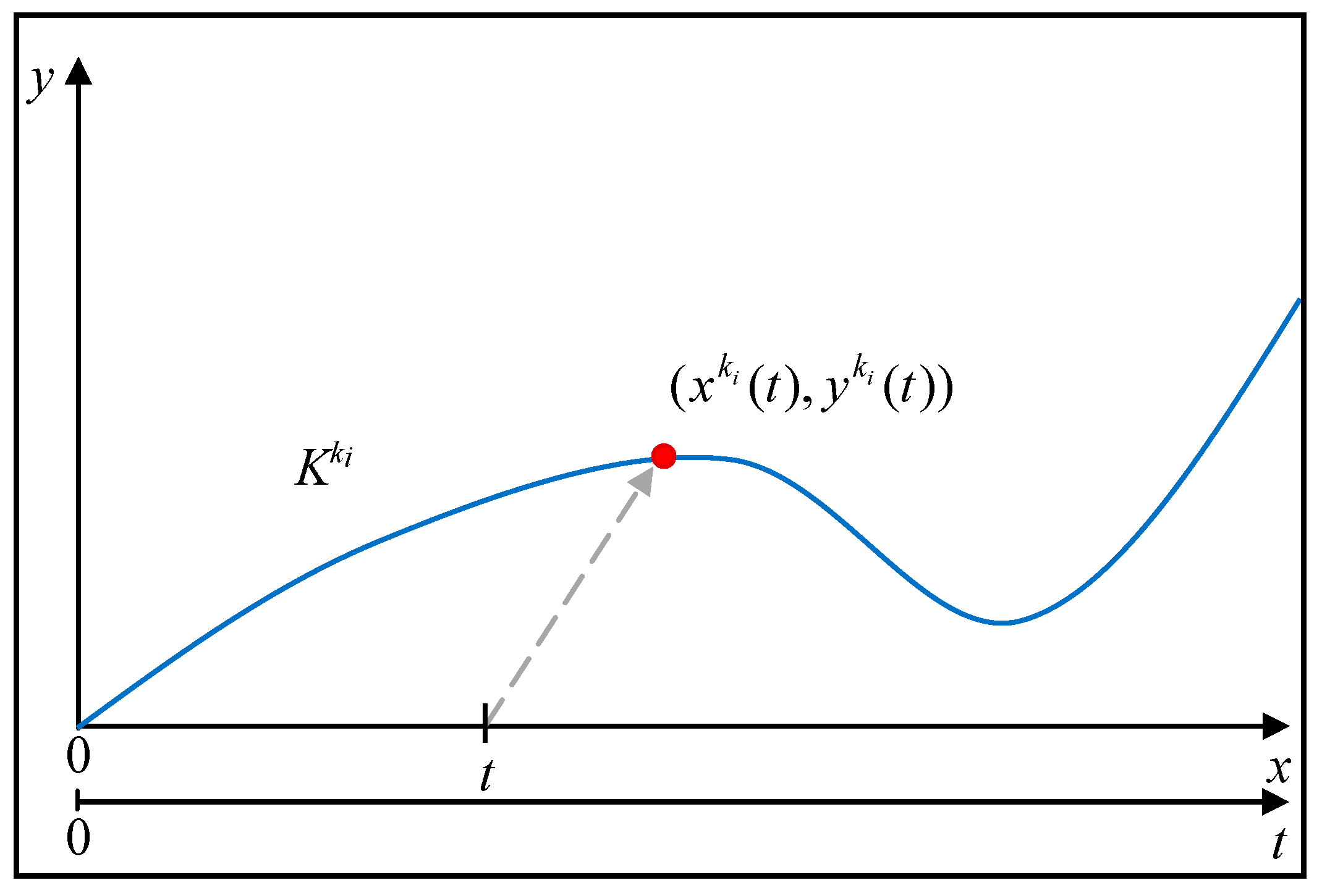
The points ( ), t ∈ 〈0,T〉, ki = 1, 2, …,~m, create a curve Kk called an oil spill central point drift trend (CPDT)
where x, y are given in meters. An exemplary CPDT is presented in Figure 9.
Therefore, assuming CPDT at each state the sequence of oil spill domains is given as follows
with the step of time ∆t, where , for t equals to (si–1 + 1)∆t, (si–1+ 2)∆t, …, si∆t, are given by
The sequence (6) is determined for the experiment time T in the successive intervals ((si–1 + 1)∆t, si∆t〉 at state ki, with si that satisfy the inequality
where and tkj kj + 1 = (h), j, = 1, 2, …,i, i = 1, 2, …, n, are the inverse functions of the conditional distribution functions Wkj kj + 1(t) and h is a number that is randomly generated over the interval 〈0, 1).
In the experiment, the considered domain is described by combining the determined domains of the sequences (6). The resulting domain represents the total extent under investigation:
with:
- c2 = −2ln(1 − p);
- expected values
- standard deviations
with radiuses
- correlation coefficients ,
for ai = 1, 2, …, bi, bi = 1, 2, …, si − si–1, i = 1, 2, …, n.
4. Application
Based on the statistical data presented in Section 2.2 and utilizing the input data from Section 2.3, the application of the algorithm outlined in Section 3 becomes possible. By employing the Monte Carlo approach, as described in references [19,26,35,62,63,64], it becomes feasible to predict the changes in the shape of the oil spill domain and forecast the trajectory of the oil under varying h-m conditions for the open water area of the Baltic Sea.
4.1. Experiment
We arbitrarily assume that the points , t ∈ 〈0,48〉, ki ∈ {1, 2, …, 6}, i = 1, 2, …, n, create an oil spill CPDT composed of curves Kki, i = 1, 2, …, n [40,65,66]. According to (5), we have
By repeatedly applying the procedure outlined in Section 3 with a time step of ∆t = 1 h, the domain that we are looking for can be obtained. This can be determined based on arbitrarily assumed standard deviations and the correlation coefficient of the coordinates of the oil spill CPDT and the radiuses of the domain, as specified in references [50,67,68]:
- = = = 0.1 + 0.2∙t;
- = 0.8;
- 0.5 + 0.5∙t,
for t ∈ 〈0,48〉, ki ∈ {1, 2, …, 6}, i = 1, 2, …, n, that in the real practice should be statistically identified using the methods given in [40].
First, a random number q is generated from the uniform distribution on the interval 〈0,1), and in this case q ≅ 0.62. Next, the initial state k1, where k1 ∈ {1, 2, …, 6}, is selected according to (3), resulting in k1(0.62) = 2.
Subsequently, another random number g is drawn, and in this case, g ≅ 0.45. With the fixed k1 = 2, we determine the next state k2, where k2 ∈ {1, 2, …, 6}, using Equation (4), i.e., k2(0.45) = 1.
Afterwards, a random number h is drawn, and in this case, h ≅ 0.20. Considering the fixed states k1 = 2 and k2 = 1, we generate the first realization tkiki + 1 = of θk1k2 from an assigned probability distribution, as indicated in Figure 6 and Figure 7. In this example, = t21 = 6.78. Consequently, we have (s1 − 1) < 6.78 ≤ s1.
Hence, s1 = 7 and s0 = 0, s1 − s0 = s1 = 7. Subsequently, we compare the value of s1 with time T, which is equal to 48. Observing that s1 = 7, which is less than 48, we proceed to draw the sequence of domains accordingly:
where
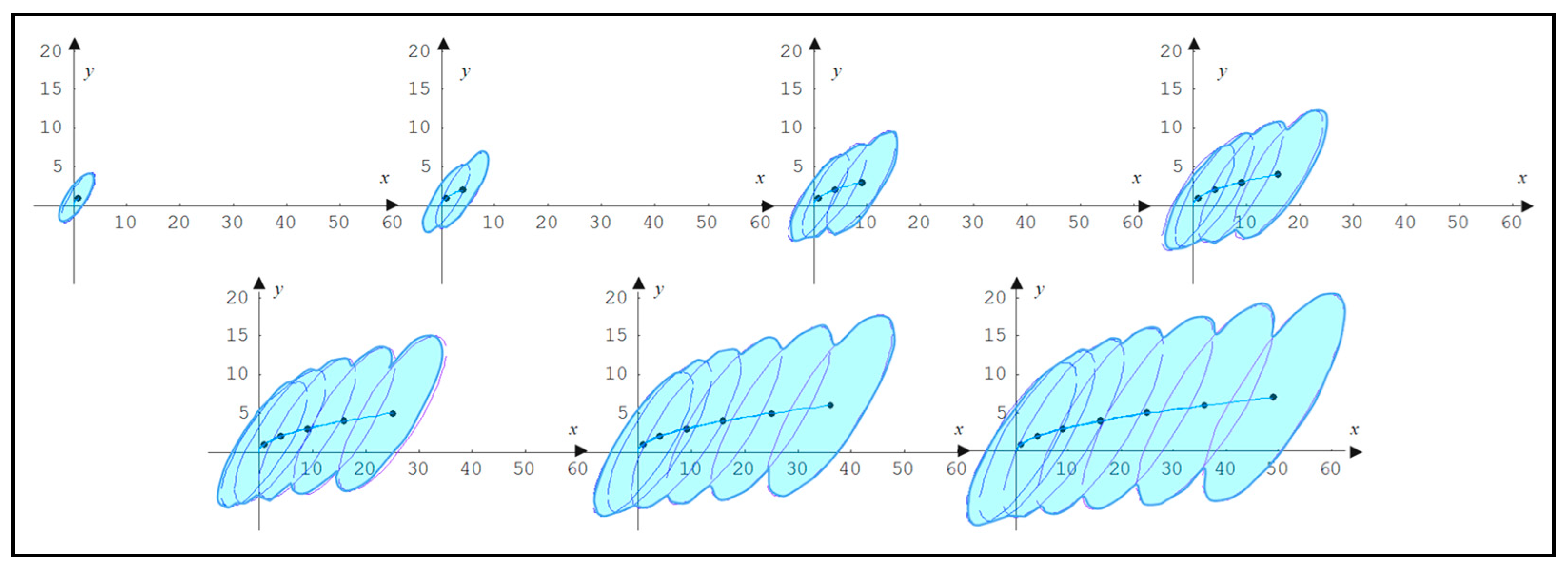
for a1 = 1, 2, …, b1, b1 = 1, 2, …, 7, composed of the elliptical sub-domains shown in Figure 10.
Further, the substitution of k2 = 1 is proceeded by randomly generating another set of numbers, g ≅ 0.76 and h ≅ 0.30. We select state k3(0.76) = 2, and generate another realization, = t12 = 18.75, for the conditional sojourn time. Once we have these realizations, we calculate their sum:
Considering the inequality (s2 − 1) < 25.53 ≤ s2, we deduce that s2 = 26 and the difference s2 − s1 = 26 − 7 = 19. Next, we compare s2 with time T and observe that s2 = 26, which is less than 48. Consequently, we obtain the sequence:
of domains, where
for a2 = 1, 2, …, b2, b2 = 1, 2, …, 19.
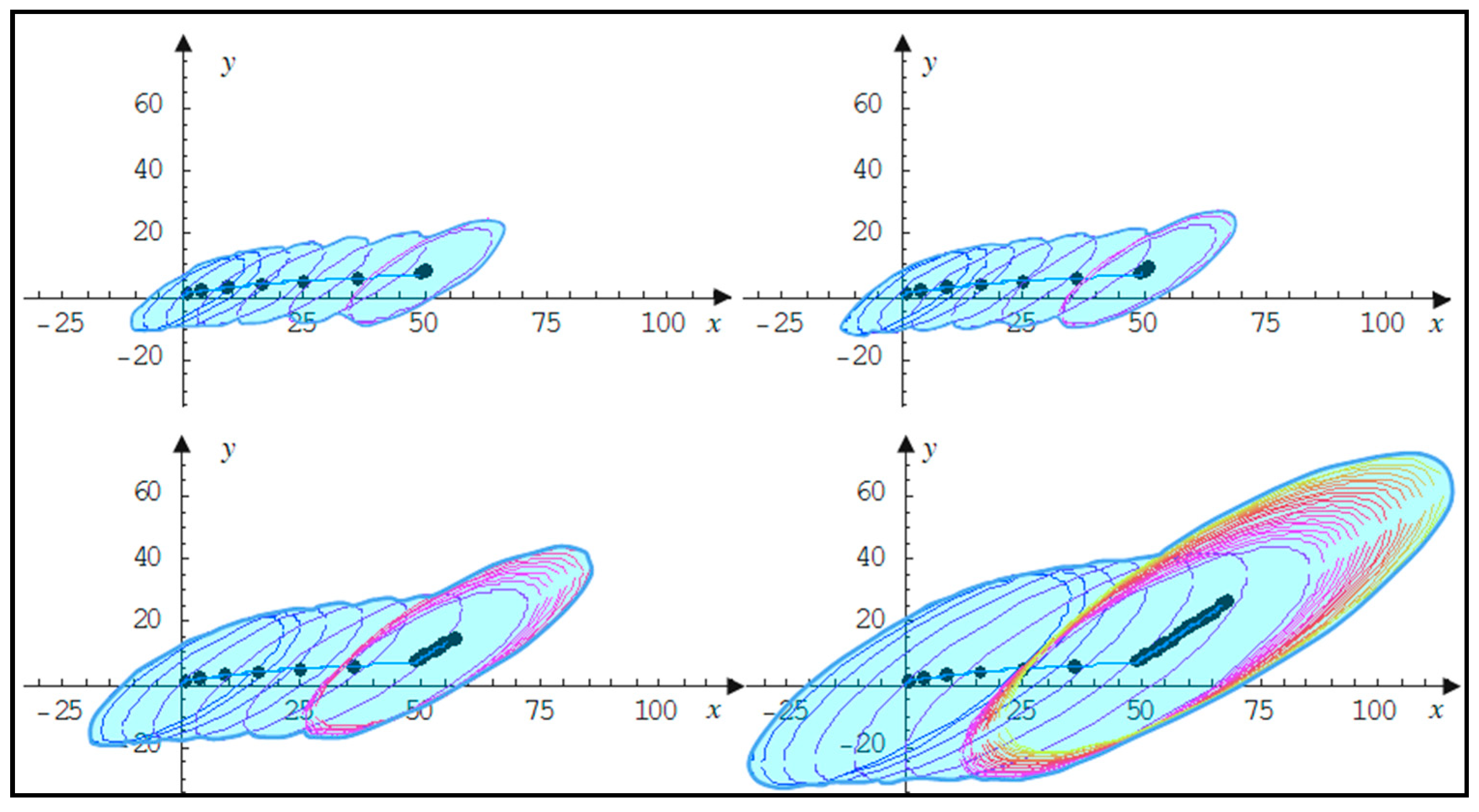
The sequence of oil spill domains in the time interval 〈s1, s2) = (7, 26〉 is partly illustrated for selected t = 8 h, 9 h, 15 h, 26 h, as shown in Figure 11. We can notice that it consists of elliptical sub-domains with bigger radiuses than those shown in Figure 10.
In the next step, we generate random numbers, g ≅ 0.03 and h ≅ 0.80. By selecting the state k4(0.03) = 1, we then obtain a realization as = 52.3. The entire sojourn time is:
and (s3 − 1) < 77.83 ≤ s3.
As s3 is greater than the experimental time 48 h, we substitute and calculate the difference s3 − s2 = 48 − 26 = 22. Based on this, we accordingly proceed to draw the sequence
of domains, where
for a3 = 1, 2, …, b3, b3 = 1, 2, …, 22.
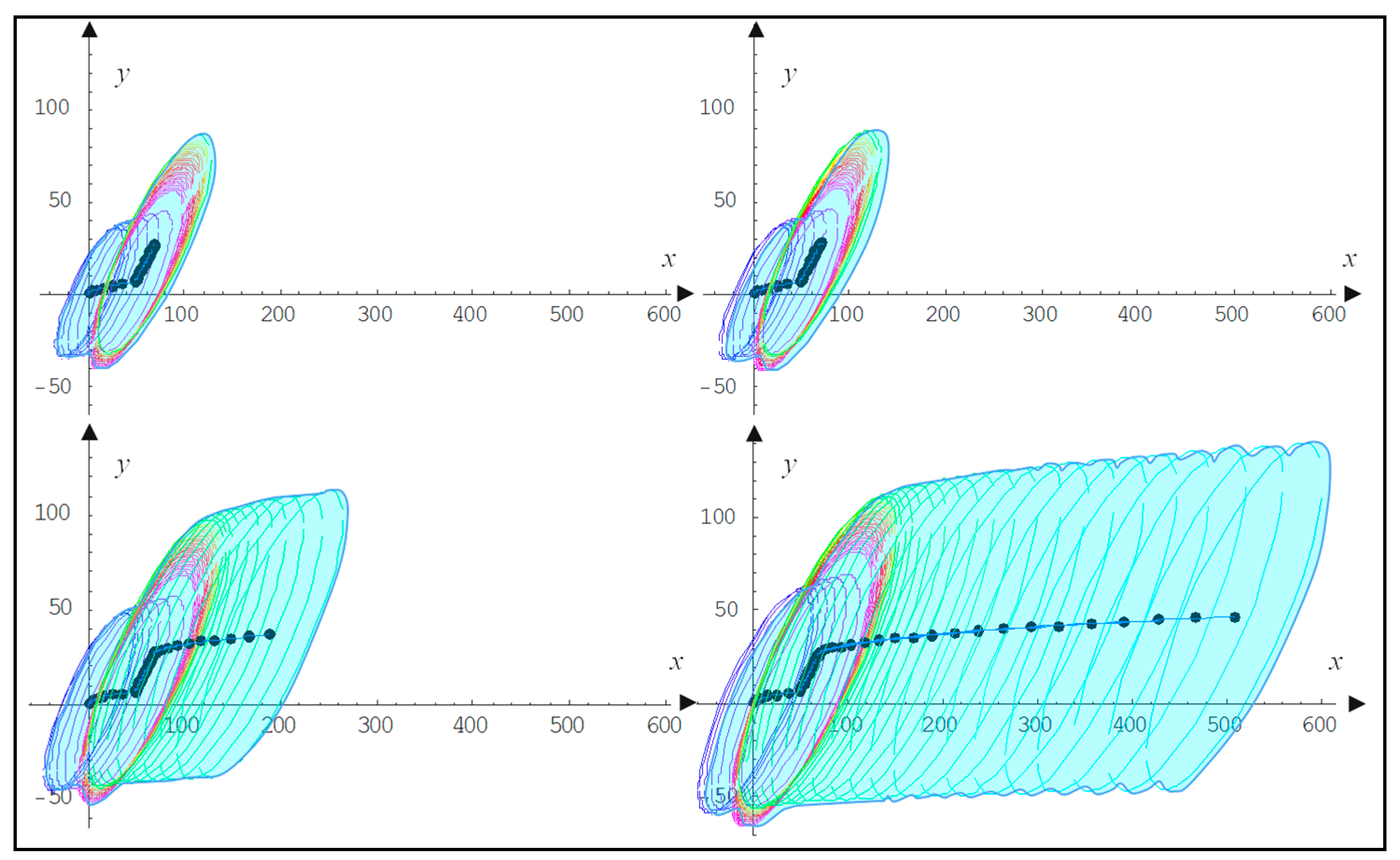
The sequence of oil spill domains (composed of the elliptical sub-domains) in the time interval 〈s3, s4) = (26, 48〉 is partly illustrated for selected t = 27 h, 28 h, 38 h, 47 h in Figure 12. Figure 13 displays the final domain at t = 48 h. The sequence for varying h-m conditions after two days of the oil discharge is presented. The simulation time can be increased and for this purpose the algorithm should be continued, i.e., the process involves substituting i with j and subsequently drawing new random numbers g, h. This is conducted to select the states ki+1 and generate different realizations . This is iteratively repeated until the cumulative sum tkjkj+1 obtained from all the generated realizations reach a new increased experiment time T. Then, the necessary parameters can be calculated and by following the aforementioned iteration process, sequences of domains under varying h-m conditions can be obtained. In the experiment, the oil spill domain is represented by the cumulative sum of sub-domains of an ellipse shape.
4.2. Discussion of Results and Further Developments
The preliminary results are obtained for arbitrarily assumed expressions of expected values and standard deviations and , correlation coefficients of the oil spill CPDT curves Kki, its equation, and the radiuses of the moving oil spill elliptical sub-domains. In the real practice, the unknown parameters should be statistically identified.
Figure 13 presents the final domain for a single simulation trial. To enhance the algorithm and simulation procedure, it is feasible to repeat the trials multiple times and calculate the average domain. This approach allows for a more comprehensive analysis and a better understanding of the overall behaviour of the oil spill.
The author aims to conduct a practical scientific experiment in specific water areas of the Baltic Sea with the intention of statistically identifying the unknown parameters associated with the assumed elements of the model proposed. This ambitious endeavour seeks to determine the forms of these model components under fixed hydro-meteorological conditions in the sea area. The insights gained from this study can be used to predict spill domains in other sea water areas with similar conditions. However, the experiments at the considered sea water areas will consume much time and cost, especially if performed for different kinds of spills and also including the physical oil characteristics and other processes, such us evaporation, emulsification, and thickness of the oil spill layer. The simulation results of the oil slick domain in terms of moving trajectories can be developed to ensure the greatest precision and correspondence to reality as possible.
5. Conclusions
This paper reports work that is of interest for practical safety in wide water areas. It proposes the utilization of the simulation technique, which employs a stochastic approach, for determining the trajectory of oil spills and investigating their horizontal domain movement. A probabilistic model is introduced and identified for the process of changing hydro-meteorological conditions at the water surface. A two-dimensional stochastic process is then employed to determine the central point position of the spill domain, and parametric equations for its trend curves under different h-m conditions are defined. Using the aforementioned approach, a comprehensive simulation algorithm is formulated to simulate the stochastic movement of oil spills within a dynamic hydro-meteorological environment. This algorithm takes into account the changing conditions over time. The practical application is demonstrated by applying it to the open water area of the Baltic Sea as a specific case study. The study specifically emphasizes two significant parameters: wave height and wind speed. By considering these factors, the algorithm provides insights into the movement patterns of oil in response to variations in h-m conditions. After successful uniformity testing and joining realisations of conditional sojourn times from different experiments or datasets into new sets of data, the unknown parameters investigation methods were applied and the simulation technique used. The prediction of oil spill movement and spreading in varying hydro-meteorological conditions is performed through determining the trajectory and movement of the oil spill domain composed of changing its surface elliptical sub-domains in time. The final result is obtained after reaching a fixed experiment time T.
The model presented in this paper serves as a valuable tool in the case of spills in areas of various oceans, seas, and inland water. The proposed simulation algorithm for oil spill domain movement investigation is universal in the sense that we can apply it in similar areas of the Baltic Sea with comparable hydro-meteorological conditions after the necessary identification of statistical model parameters through the scientific experiment. Transferring the findings to other water regions that share similar h-m conditions would undoubtedly enhance and optimize environmental protection efforts. This method provides a rapid and precise means of determining oil discharge trajectories and predicting their domain movement. The research outcomes obtained from this study serve as initial results in the field of oil spill simulation.
As oil spills can have a profound impact on the reliability of operations, profitability of investments, and operating costs associated with various industries and sectors [69,70], it seems reasonable to devote significant attention and resources to prevent and effectively respond to oil discharges, ensuring the sustainability and resilience of these industries in the face of potential environmental risks. Moreover, the aviation industry, with its reliance on fuel and oil can have the potential impact on oil spills [71,72]. Investing in early warning systems and improving spill response capabilities can help minimize the impact of e.g., flood-induced oil spills [73]. The method proposed in the paper can be applied to various types of spills, thereby mitigating the detrimental consequences for the environment.
Funding
This research received no external funding.
Data Availability Statement
The data presented in this study are available on request from the author, excluding some data protected by copyright.
Conflicts of Interest
The author declares no conflict of interest.
References
- Fingas, M. Oil Spill Science and Technology, 2nd ed.; Elsevier: Amsterdam, The Netherlands, 2016. [Google Scholar]
- Eckroth, J.R.; Madsen, M.M.; Hoell, E. Dynamic Modeling of Oil Spill Cleanup Operations. In Proceedings of the 38th AMOP Technical Seminar on Environmental Contamination and Response, Vancouver, BC, Canada, 2–4 June 2015; pp. 16–35. [Google Scholar]
- Federal Register. Rules and Regulations. § 254.6—Definitions. Federal Register, 18 October 2011, Volume 76.
- Cordes, E.E.; Jones, D.O.B.; Schlacher, T.A.; Amon, D.J.; Bernardino, A.F.; Brooke, S.; Carney, R.; DeLeo, D.M.; Dunlop, K.M.; Escobar-Briones, E.G.; et al. Environmental Impacts of the Deep-Water Oil and Gas Industry: A Review to Guide Management Strategies. Front. Environ. Sci. 2016, 4, 58. [Google Scholar] [CrossRef]
- The International Tanker Owners Pollution Federation Limited (ITOPF). Promoting Effective Spill Response, Oil Tanker Spill Statistics 2022; The International Tanker Owners Pollution Federation Limited (ITOPF): London, UK, 2023. [Google Scholar]
- Pocora, A.; Purcarea, A.A.; Nicolae, F.; Cotorcea, A. Modelling and simulation of oil spills in coastal waters. IOP Conf. Ser. Earth Environ. Sci. 2018, 172, 012012. [Google Scholar] [CrossRef]
- Dobrzycka-Krahel, A.; Bogalecka, M. The Baltic Sea under Anthropopressure—The Sea of Paradoxes. Water 2022, 14, 3772. [Google Scholar] [CrossRef]
- Nixon, Z.; Michel, J. Predictive Modeling of Subsurface Shoreline Oil Encounter Probability from the Exxon Valdez Oil Spill in Prince William Sound, Alaska. Environ. Sci. Technol. 2015, 49, 4354–4361. [Google Scholar] [CrossRef]
- Bogalecka, M. Consequences of maritime critical infrastructure accidents with chemical releases. Int. J. Mar. Navig. Saf. Sea Transp. 2019, 13, 771–779. [Google Scholar] [CrossRef]
- Bogalecka, M. Consequences of Maritime Critical Infrastructure Accidents. Environmental Impacts Modeling—Identification—Prediction—Optimization—Mitigation; Elsevier: Amsterdam, The Netherlands, 2020. [Google Scholar] [CrossRef]
- Australian Maritime Safety Authority (AMSA). Oil Spill Monitoring Handbook; Wardrop Consulting and the Cawthron Institute for the Australian Maritime Safety Authority (AMSA); Marine Safety Authority of New Zealand (MSA): Canberra, Australia, 2003. [Google Scholar]
- Etkin, D.S. Estimating Cleanup Costs for Oil Spills. In Proceedings of the 1999 International Oil Spill Conference Proceedings, Seattle, WA, USA, 7–12 March 1999; p. 168. [Google Scholar]
- Kontovas, C.A.; Ventikos, N.P.; Psaraftis, H.N. Estimating the Consequences Costs of Oil Spills from Tankers. In Proceedings of the SNAME 2011 Annual Meeting, Houston, TX, USA, 16–18 November 2011. [Google Scholar]
- Nikula, P.; Tynkkynen, V.P. Oil Transportation and Maritime Safety. In Towards a Baltic Sea Region Strategy in Critical Infrastructure Protection; Pursiainen, C., Ed.; Nordregio: Stockholm, Sweden, 2007; Volume 5, pp. 141–164. [Google Scholar]
- Ornitz, B.; Champ, M. Oil Spills First Principles: Prevention and Best Response; Elsevier: Amsterdam, The Netherlands, 2002. [Google Scholar]
- Armenio, E.; Ben Meftah, M.; De Padova, D.; De Serio, F.; Mossa, M. Monitoring Systems and Numerical Models to Study Coastal Sites. Sensors 2019, 19, 1552. [Google Scholar] [CrossRef] [PubMed]
- Bogalecka, M.; Dąbrowska, E. Monte Carlo Simulation Approach to Shipping Accidents Consequences Assessment. Water 2023, 15, 1824. [Google Scholar] [CrossRef]
- Dąbrowska, E.; Kołowrocki, K. Probabilistic Approach to Determination of Oil Spill Domains at Port and Sea Water Areas. TransNav Int. J. Mar. Navig. Saf. Sea Transp. 2020, 14, 51–58. [Google Scholar] [CrossRef]
- Kim, T.; Yang, C.-S.; Ouchi, K.; Oh, Y. Application of the method of moment and Monte-Carlo simulation to extract oil spill areas from synthetic aperture radar images. In Proceedings of the 2013 OCEANS—San Diego, San Diego, CA, USA, 23–27 September 2013; pp. 1–4. [Google Scholar]
- Jernelöv, A. The threats from oil spills: Now, then, and in the future. Ambio 2010, 39, 353–366. [Google Scholar] [CrossRef] [PubMed]
- Kulygin, V.V. A review of modern approaches of oil spill modelling. In Proceedings of the International Conference on Oil and Gas of Arctic Shelf, Murmansk, Russia, 2006. [Google Scholar]
- Zafirakou, A.; George, P.; Samaras, A.; Koutitas, C. Oil Spill Modeling Aiming at the Protection of Ports and Coastal Areas. Environ. Process. 2015, 2, 41–53. [Google Scholar] [CrossRef]
- Adofo, Y.K.; Nyankson, E.; Agyei-Tuffour, B. Dispersants as an oil spill clean-up technique in the marine environment: A review. Heliyon 2022, 8, e10153. [Google Scholar] [CrossRef] [PubMed]
- Oil Spill Prevention and Response Technical Advisory Committee (TAC). Minutes of the Meeting of 8 January 2016; California Department of Fish and Wildlife Office of Spill Prevention and Response: Sacramento, CA, USA, 2016. [Google Scholar]
- Fay, J.A. Physical Processes in the Spread of Oil on a Water Surface. In Proceedings of the Joint Conference on Prevention and Control of Oil Spills, sponsored by American Petroleum Industry, Environmental Protection Agency, and United States Coast Guard, Washington, DC, USA, 15–17 June 1971; pp. 463–468. [Google Scholar]
- Huang, J.C. A review of the state-of-the-art of oil spill fate/behavior models. In Proceedings of the International Oil Spill Conference Proceedings, San Antonio, TX, USA, 28 February–3 March 1983; Volume 1983, pp. 313–322. [Google Scholar]
- American Society of Civil Engineers (ASCE) Task Committee on Modeling of Oil Spills. State-of-the-art review of modelling transport and fate of oil spills. J. Hydraul. Eng. 1996, 122, 594–609. [Google Scholar] [CrossRef]
- Chen, C.S.; Huang, H.S.; Beardsley, R.C.; Liu, H.; Xu, Q. A finite volume numerical approach for coastal ocean circulation studies: Comparisons with finite difference models. J. Geophys. Res. 2007, 112, C3018. [Google Scholar] [CrossRef]
- De Dominicis, M.; Pinardi, N.; Zodiatis, G.; Lardner, R. MEDSLIK-II, a Lagrangian marine surface oil spill model for short-term forecasting—Part 1: Theory. Geosci. Model Dev. 2013, 6, 1851–1869. [Google Scholar] [CrossRef]
- Etkin, D.S.; Michel, J.; McCay, D.F.; Boufadel, M.; Li, H. Integrating state-of-the-art shoreline interaction knowledge into spill modeling. In Proceedings of the International Oil Spill Conference Proceedings, Savannah, GA, USA, 4–8 May 2008; pp. 915–922. [Google Scholar]
- Periáñez, R. Chemical and oil spill rapid response modelling in the Strait of Gibraltar-Alborán Sea. Ecol. Model. 2007, 207, 210–222. [Google Scholar] [CrossRef]
- Periáñez, R.; Pascual-Granged, A. Modelling surface radioactive, chemical and oil spills in the Strait of Gibraltar. Comput. Geosci. 2008, 34, 163–180. [Google Scholar] [CrossRef]
- Spaulding, M.L. A state-of-the-art review of oil spill trajectory and fate modeling. Oil Chem. Pollut. 1989, 4, 39–55. [Google Scholar] [CrossRef]
- Volckaert, F.; Tombroff, D. Progress Report to EEC Div. XI/B/l; IntechOpen Limited: London, UK, 1989. [Google Scholar]
- Wang, J.; Shen, Y. Development of an integrated model system to simulate transport and fate of oil spills in seas. Sci. China Technol. Sci. 2010, 53, 2423–2434. [Google Scholar] [CrossRef]
- Lehr, W.; Simecek-Beatty, D.; Aliseda, A.; Boufadel, M. Review of Recent Studies on Dispersed Oil Droplet Distribution. In Proceedings of the 37th AMOP Technical Seminar on Environmental Contamination and Response, Canmore, AB, Canada, 3–5 June 2014; pp. 1–8. [Google Scholar]
- McCay, D.F.; Reich, D.; Michel, J.; Etkin, D.; Symons, L.; Helton, D.; Wagner, J. Oil spill consequence analyses of potentially-polluting shipwrecks. In Proceedings of the 35th AMOP Technical Seminar on Environmental Contamination and Response, Vancouver, BC, Canada, 5–7 June 2012; pp. 751–774. [Google Scholar]
- Dąbrowska, E. Conception of Oil Spill Trajectory Modelling: Karlskrona Seaport Area as an Investigative Example. In Proceedings of the 2021 5th International Conference on System Reliability and Safety (ICSRS), Palermo, Italy, 24–26 November 2021; Piscataway: Institute of Electrical and Electronics Engineers (IEEE). pp. 307–311. [Google Scholar]
- Dąbrowska, E.; Kołowrocki, K. Monte Carlo Simulation Approach to Determination of Oil Spill Domains at Port and Sea Waters Areas. TransNav Int. J. Mar. Navig. Saf. Sea Transp. 2020, 14, 59–64. [Google Scholar] [CrossRef]
- Dąbrowska, E.; Kołowrocki, K. Modelling, Identification and Prediction of Oil Spill Domains at Port and Sea Water Areas. J. Pol. Saf. Reliab. Assoc. Summer Saf. Reliab. Semin. 2019, 10, 43–58. [Google Scholar]
- Grabski, F. Semi-Markov Processes: Application in System Reliability and Maintenance; Elsevier: Amsterdam, The Netherlands, 2014. [Google Scholar]
- Kołowrocki, K.; Soszyńska-Budny, J. Reliability and Safety of Complex Technical Systems and Processes: Modeling—Identification—Prediction—Optimization, 1st ed.; Springer: London, UK, 2011. [Google Scholar]
- Dąbrowska, E. Monte Carlo Simulation Prediction of Oil Spill Domain Movement considering Oil Spill Layer Thickness and Changing Hydro-Meteorological Conditions Impacts. Waters, 2023; in press. [Google Scholar]
- Dąbrowska, E.; Soszyńska-Budny, J. Monte Carlo Simulation Forecasting of Maritime Ferry Safety and Resilience. In Proceedings of the 2018 IEEE International Conference on Industrial Engineering and Engineering Management—IEEM 2018, Bangkok, Thailand, 16–19 December 2018; ISBN 978-1-5386-6785-9. [Google Scholar]
- Kołowrocki, K.; Kuligowska, E. Operation and Climate-Weather Change Impact on Maritime Ferry Safety. In Safety and Reliability—Safe Societies in a Changing World; CRC Press: London, UK, 2018; pp. 849–858. ISBN 978-0-8153-8682-7. European Safety and Reliability Conference—ESREL 2018, Trondheim, Norway, 17–21 June 2018. [Google Scholar]
- Kołowrocki, K.; Kuligowska, E.; Soszyńska-Budny, J.; Torbicki, M. Safety and Risk Prediction of Port Oil Piping Transportation System Impacted by Climate-Weather Change Process. In Proceedings of the International Conference on Information and Digital Technologies 2017-IDT, Zilina, Slovakia, 5–7 July 2017; pp. 173–177, ISBN 978-1-5090-5688-0. [Google Scholar]
- Bogalecka, M.; Kołowrocki, K. Prediction of critical infrastructure accident losses of chemical releases impacted by climate-weather change. In Proceedings of the 2018 IEEE International Conference on Industrial Engineering and Engineering Management (IEEM), Bangkok, Thailand, 16–19 December 2018; pp. 788–792. [Google Scholar] [CrossRef]
- Bogalecka, M.; Kołowrocki, K. Minimization of critical infrastructure accident losses of chemical releases impacted by climate-weather change. In Proceedings of the 2018 IEEE International Conference on Industrial Engineering and Engineering Management (IEEM), Bangkok, Thailand, 16–19 December 2018; pp. 1657–1661. [Google Scholar] [CrossRef]
- Ellis, J. Analysis of accidents and incidents occurring during transport of packaged dangerous goods by sea. Saf. Sci. 2011, 49, 1231–1237. [Google Scholar] [CrossRef]
- Elliot, A.; Hurford, N.; Penn, C. Shear diffusion and the spreading of slicks. Mar. Pollut. Bull. 1986, 17, 308–313. [Google Scholar] [CrossRef]
- Bruno, M.F.; Molfetta, M.G.; Pratola, L.; Mossa, M.; Nutricato, R.; Morea, A.; Nitti, D.O.; Chiaradia, M.T. A Combined Approach of Field Data and Earth Observation for Coastal Risk Assessment. Sensors 2019, 19, 1399. [Google Scholar] [CrossRef] [PubMed]
- Farrington, J.W. Oil Pollution in the Marine Environment II: Fates and Effects of Oil Spills. Environ. Sci. Policy Sustain. Dev. 2014, 56, 16–31. [Google Scholar] [CrossRef]
- Hryniewicz, O.; Kaczmarek-Majer, K. Monitoring of Possibilisticaly Aggregated Complex Time Series. In Building Bridges Between Soft and Statistical Methodologies for Data Science. In Proceedings of 10th International Conference on Soft Methods in Probability and Statistics (SMPS), Valladolid, Spain, 14–16 September 2022; Advances in Intelligent Systems and Computing; Garcia-Escudero, L.A., Gordaliza, A., Mayo, A., Gomez, M.A.L., Gil, M.A., Grzegorzewski, P., Hryniewicz, O., Eds.; Springer Nature: Cham, Swizerland, 2023; pp. 208–215. [Google Scholar] [CrossRef]
- Van Belle, J.; van Barneveld-Biesma, J.; Bastiaanssen, V.; Buitenhuis, A.; Saes, L.; van Veen, G. ICOS Impact Assessment Report; Technopolis: Amsterdam, The Netherlands, 2018; pp. 48–51. [Google Scholar]
- EU-CIRCLE Report D2.3-GMU2. Identification Methods and Procedures of Climate-Weather Change Process Including Extreme Weather Hazards. 2016. Available online: http://jpsra.am.gdynia.pl/ (accessed on 16 May 2023).
- Gdynia Maritime University Safety Interactive Platform. Available online: http://gmu.safety.umg.edu.pl/ (accessed on 1 June 2022).
- Kołowrocki, K.; Kuligowska, E.; Soszyńska-Budny, J.; Torbicki, M. Simplified Impact Model of Critical Infrastructure Safety Related to Climate-Weather Change Process. In Proceedings of the International Conference on Information and Digital Technologies 2017-IDT, Zilina, Slovakia, 5–7 July 2017; pp. 187–190, ISBN 978-1-5090-5688-0. [Google Scholar]
- Kołowrocki, K.; Soszyńska-Budny, J.; Torbicki, M. Critical Infrastructure Impacted by Climate Change Safety and Resilience Indicators. In Proceedings of the 2018 IEEE International Conference on Industrial Engineering and Engineering Management (IEEM), Bangkok, Thailand, 16–19 December 2018; pp. 986–990. [Google Scholar] [CrossRef]
- Kuligowska, E.; Torbicki, M. Climate-weather change process realizations uniformity testing for maritime ferry operating area. In Proceedings of the Applied Stochastic Models and Data Analysis International Conference with Demographics Workshop—ASMDA 2017, London, UK, 6–9 June 2017; pp. 605–618. [Google Scholar]
- Kuligowska, E.; Torbicki, M. Identification and prediction of climate-weather change processes for port oil piping transportation system and maritime ferry operation areas after their realisations successful uniformity testing. In Proceedings of the Applied Stochastic Models and Data Analysis International Conference with Demographics Workshop—ASMDA 2017, London, UK, 6–9 June 2017; pp. 621–630. [Google Scholar]
- Torbicki, M. Longtime Prediction of Climate-Weather Change Influence on Critical Infrastructure Safety and Resilience. In Proceedings of the 2018 IEEE International Conference on Industrial Engineering and Engineering Management (IEEM), Bangkok, Thailand, 16–19 December 2018; pp. 996–1000. [Google Scholar] [CrossRef]
- Marseguerra, M.; Zio, E. Basics of the Monte Carlo Method with Application to System Reliability; LiLoLe: Hagen, Germany, 2002. [Google Scholar]
- Rao, M.S.; Naikan, V.N.A. Review of simulation approaches in reliability and availability modeling. Int. J. Perform. Eng. 2016, 12, 369–388. [Google Scholar]
- Law, A.M. Simulation Modelling and Analysis, 5th ed.; McGraw Hill Education: New York, NY, USA, 2000; ISBN 978-0-07-340132-4. [Google Scholar]
- National Oceanic and Atmospheric Administration (NOAA). Response Tools for Oil Spills. Available online: http://response.restoration.noaa.gov/oil-and-chemical-spills/oil-spills/response-tools/response-tools-oil-spills.html/ (accessed on 30 May 2022).
- National Oceanic and Atmospheric Administration (NOAA). Trajectory Analysis Handbook. NOAA Hazardous Material Response Division. Seattle: WA. Available online: http://www.response.restoration.noaa.gov/ (accessed on 30 May 2022).
- Horn, M.; French-McCay, D. Trajectory and fate modeling with acute effects assessment of hypothetical spills of diluted bitumen into rivers. In Proceedings of the 38th AMOP Technical Seminar on Environmental Contamination and Response, Vancouver, BC, Canada, 2–4 June 2015; pp. 549–581. [Google Scholar]
- Johansen, T.; Reed, M.; Boksburg, N.R. Natural dispersion revisited. Mar. Pollut. Bull. 2015, 93, 20–26. [Google Scholar] [CrossRef]
- Das, T.; Goerlandt, F. Bayesian inference modeling to rank response technologies in arctic marine oil spills. Available online: https://www.sciencedirect.com/science/article/abs/pii/S0025326X22008852 (accessed on 16 May 2023).
- Kut, P.; Pietrucha-Urbanik, K. Most Searched Topics in the Scientific Literature on Failures in Photovoltaic Installations. Energies 2022, 15, 8108. [Google Scholar] [CrossRef]
- Toruń, A.; Burniak, C.; Biały, J.; Tomaszewska, J.; Grzesik, N.; Hošková-Mayerová, Š.; Woch, M.; Zieja, M.; Rurak, A. Challenges for Air Transport Providers in Czech Republic and Poland. J. Adv. Transp. 2018, 6374592, 1–7. [Google Scholar] [CrossRef]
- Woch, M.; Zieja, M.; Tomaszewska, J. Analysis of the Time between Failures of Aircrafts. In Proceedings of the 2017 2th International Conference on System Reliability and Safety (ICSRS), Milan, Italy, 20–22 December 2017; pp. 112–118, ISBN 978-1-5386-3320-5. [Google Scholar]
- Eldeeb, H.M.; Ibrahim, A.; Mowafy, M.H.; Zeleňáková, M.; Abd-Elhamid, H.F.; Pietrucha-Urbanik, K.; Ghonim, M.T. Assessment of Dams’ Failure and Flood Wave Hazards on the Downstream Countries: A Case Study of the Grand Ethiopian Renaissance Dam (GERD). Water 2023, 15, 1609. [Google Scholar] [CrossRef]
Figure 1.
Numbers of tanker spills (medium and large). Source: Own elaboration adapted with permission from Ref. [5].
Figure 1.
Numbers of tanker spills (medium and large). Source: Own elaboration adapted with permission from Ref. [5].

Figure 2.
Number of tanker spills and quantities of oil discharge (medium and large) in the recent years. Source: Own elaboration adapted with permission from Ref. [5].
Figure 2.
Number of tanker spills and quantities of oil discharge (medium and large) in the recent years. Source: Own elaboration adapted with permission from Ref. [5].

Figure 3.
Assumptions and denotations. Source: Own elaboration.

Figure 4.
Selected Baltic Sea waterway at the Bornholm Basin between two ports (blue line) with highlighted hydro-meteotological measurement points [55].
Figure 4.
Selected Baltic Sea waterway at the Bornholm Basin between two ports (blue line) with highlighted hydro-meteotological measurement points [55].

Figure 5.
Exemplary realization of the process A(t). Source: Own elaboration.

Figure 6.
Verified distribution functions of conditional sojourn times.

Figure 7.
Empirical distribution functions of conditional sojourn times.

Figure 8.
Algorithm of oil spill drift for varying h-m conditions.

Figure 9.
Curve Kk of CPDT.

Figure 10.
The sequence of oil spill domains at the moments t = 1 h, 2 h, …, 7 h.

Figure 11.
The sequence of domains at the moments t = 8 h, 9 h, 15 h, 26 h.

Figure 12.
The sequence of domains at the moments t = 27 h, 28 h, 37 h, 47 h.

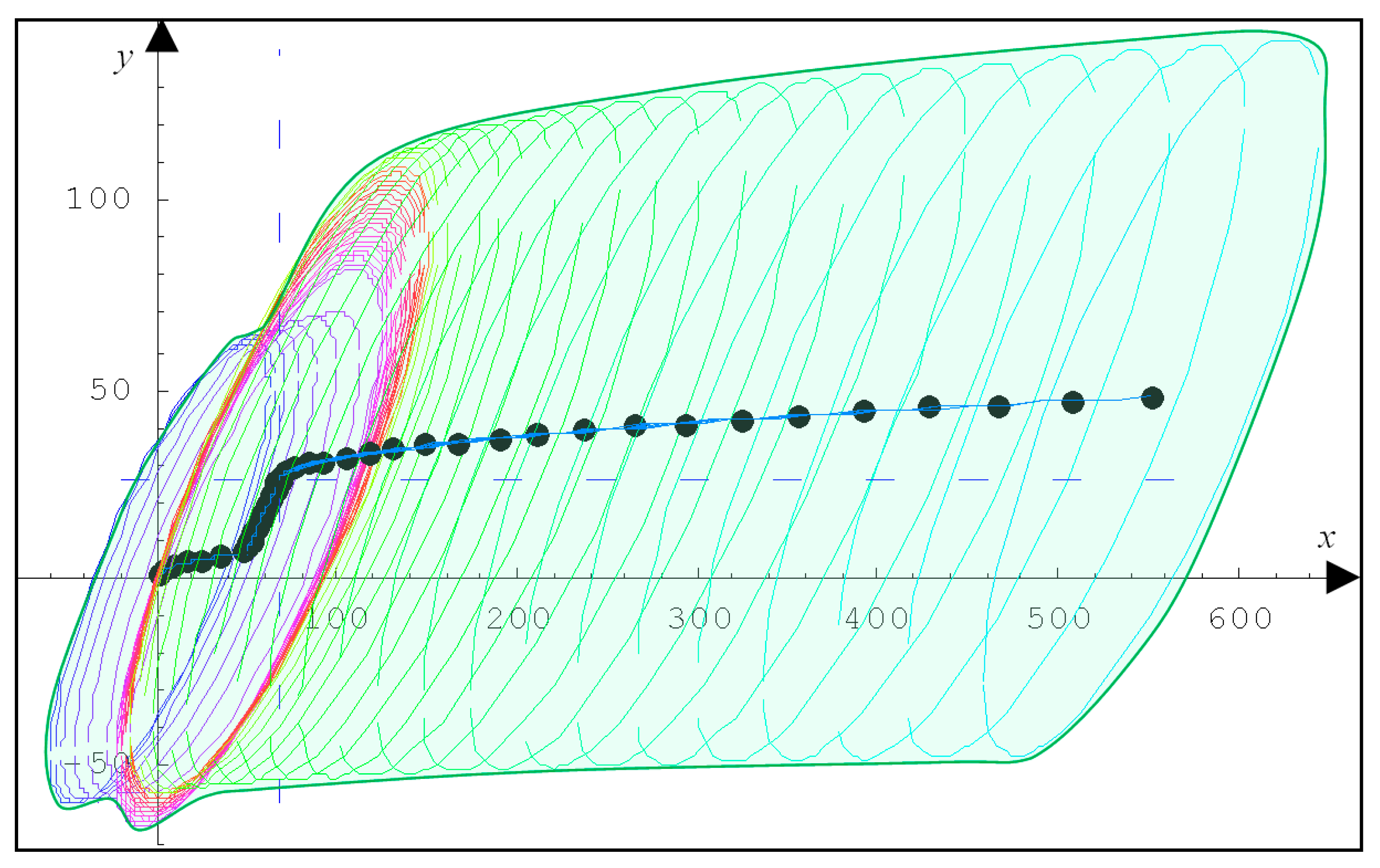
Figure 13.
The final oil spill domain at the moment t = 48 h.


Table 1.
States of the process of varying h-m conditions for selected Baltic Sea open waters area.
| States | wh [m] | ws [m/s] |
|---|---|---|
| 1 | 0–2 | 0–17 |
| 2 | 2–5 | 0–17 |
| 3 | 5–14 | 0–17 |
| 4 | 0–2 | 17–33 |
| 5 | 2–5 | 17–33 |
| 6 | 5–14 | 17–33 |
Table 2.
Numbers of initial realisations of the process.
| State | 1 | 2 | 3 | 4 | 5 | 6 | Total |
|---|---|---|---|---|---|---|---|
| ni | 405 | 237 | 0 | 0 | 27 | 11 | 680 |
Table 3.
The numbers of transitions between the states.
| State | 1 | 2 | 3 | 4 | 5 | 6 |
|---|---|---|---|---|---|---|
| 1→ | – | 1516 | 0 | 1 | 31 | 0 |
| 2→ | 1001 | – | 0 | 0 | 435 | 0 |
| 3→ | 0 | 11 | – | 0 | 1 | 0 |
| 4→ | 0 | 0 | 0 | – | 1 | 0 |
| 5→ | 0 | 298 | 2 | 0 | – | 88 |
| 6→ | 0 | 45 | 16 | 0 | 48 | – |
Disclaimer/Publisher’s Note: The statements, opinions and data contained in all publications are solely those of the individual author(s) and contributor(s) and not of MDPI and/or the editor(s). MDPI and/or the editor(s) disclaim responsibility for any injury to people or property resulting from any ideas, methods, instructions or products referred to in the content. |
© 2023 by the author. Licensee MDPI, Basel, Switzerland. This article is an open access article distributed under the terms and conditions of the Creative Commons Attribution (CC BY) license (https://creativecommons.org/licenses/by/4.0/).
Share and Cite
MDPI and ACS Style
Dąbrowska, E. Oil Discharge Trajectory Simulation at Selected Baltic Sea Waterway under Variability of Hydro-Meteorological Conditions. Water 2023, 15, 1957. https://doi.org/10.3390/w15101957
AMA Style
Dąbrowska E. Oil Discharge Trajectory Simulation at Selected Baltic Sea Waterway under Variability of Hydro-Meteorological Conditions. Water. 2023; 15(10):1957. https://doi.org/10.3390/w15101957
Chicago/Turabian StyleDąbrowska, Ewa. 2023. "Oil Discharge Trajectory Simulation at Selected Baltic Sea Waterway under Variability of Hydro-Meteorological Conditions" Water 15, no. 10: 1957. https://doi.org/10.3390/w15101957
Note that from the first issue of 2016, this journal uses article numbers instead of page numbers. See further details here.