
Pollution and Climatic Influence on Trees in the Siberian Arctic Wetlands
by
 , , , , and
Viacheslav I. Kharuk
1,2,3 ,
,
Il’ya A. Petrov
1,2,3,*,
Sergei T. Im
1,2,3,4,
Alexey S. Golyukov
1,2,3,
Maria L. Dvinskaya
1,3 and
Alexander S. Shushpanov
1,3,4 1
Sukachev Institute of Forests, Federal Scientific Center, Russian Academy of Science, Siberian Branch, Academgorodok 50/28, Krasnoyarsk 660036, Russia
2
School of Space and Information Technologies and School of Ecology and Geography, Siberian Federal University, Svobodny Str. 79, Krasnoyarsk 660041, Russia
3
Laboratory of Biodiversity and Ecology, Tomsk State University, Lenina Str. 36, Tomsk 634050, Russia
4
Institute of Space Research and High Technologies, Reshetnev Siberian State University of Science and Technology, Krasnoyarsky Rabochy Str. 31, Krasnoyarsk 660014, Russia
*
Author to whom correspondence should be addressed.
Water 2023, 15(2), 215; https://doi.org/10.3390/w15020215
Submission received: 25 November 2022
/
Revised: 23 December 2022
/
Accepted: 29 December 2022
/
Published: 4 January 2023
(This article belongs to the Special Issue Climate Change and Anthropogenic Impacts on Wetland Ecosystems in Siberia: Past, Present, and Future)
Abstract
:Siberian Arctic wetlands located within the planetary “warming hotspot” experience pronounced climate-driven vegetation cover changes. Together with warming, wetlands, which are located within the influence of Norilsk copper and nickel industry (69.35° N, 88.12° E), have been strongly influenced by industrial pollutions (sulfur dioxide mostly) since the 1940s. In addition, petroleum products release occurred in 2020 that potentially influenced vegetation vigor. We studied the combined effect of climate warming and pollution on the larch (Larix sibirica Ledeb.) and shrubs’ (Salix spp. and alder, Duschekia fruticosa) growth. Using satellite data (MODIS and Sentinel) processing, we mapped wetlands within the study area. We used on-ground survey, and applied dendrochronology, climate variables, and emissions rate analysis. We sampled woods (kerns) and, based on the tree ring analysis, generated trees and shrubs growth index (GI) chronologies. We analyzed the influence of the SO2 emissions and eco-climate variables (air temperatures, precipitation, soil moisture, and drought index SPEI) on the larch and shrubs GI. We mapped GPP and NPP (gross and net primary productivity) and vegetation index NDVI and temporal trends of these indexes based on the MODIS-derived products. We found that chronic SO2 influence led to larch trees GI decrease that was followed by tree mortality, which was observed until the end of 1990. Since the beginning of the 2000s, the GI of larch and shrubs has increased, which is correlated with elevated air and soil temperature and growth season prolongation, whereas excessive soil moisture negatively influenced GI. Together with that, increasing trends of vegetation indexes (GPP, NPP, and NDVI) were observed on the part of wetland within the zone of former trees’ heavy damage and mortality. The trends began mostly in 2003–2005 and were caused by emissions volume decrease and warming, together with resistant species’ (willows, graminoids, bushes, and birch) growth and invasion. We suggested that increasing productivity trends might partly be attributed to nitrogen fertilization caused by NOx emissions. Finally, we found that diesel fuel spill which happened in 2020 caused no influence on the larch, whereas some aquatic species (mosses mostly) were damaged.
1. Introduction
Northern marchlands are under a stronger influence of elevated temperatures than similar lands at lower latitudes, since the warming rate in the Arctic is more than two times higher [1]. Together, increased warming and fire activity in the permafrost area are initiating changes in the vegetation cover and species composition [2,3]. Within the Siberian Arctic, a combined warming and anthropogenic impact on the vegetation cover located within the polluted zone was caused by the Norilsk industry region. Chronical emissions (sulfur dioxide mostly) have influenced the wetland vegetation, including sparse and open forests, since the 1940s. This is a unique combination of the technogenic and climatic influence on the wetland vegetation within the completely circumpolar zone and beyond.
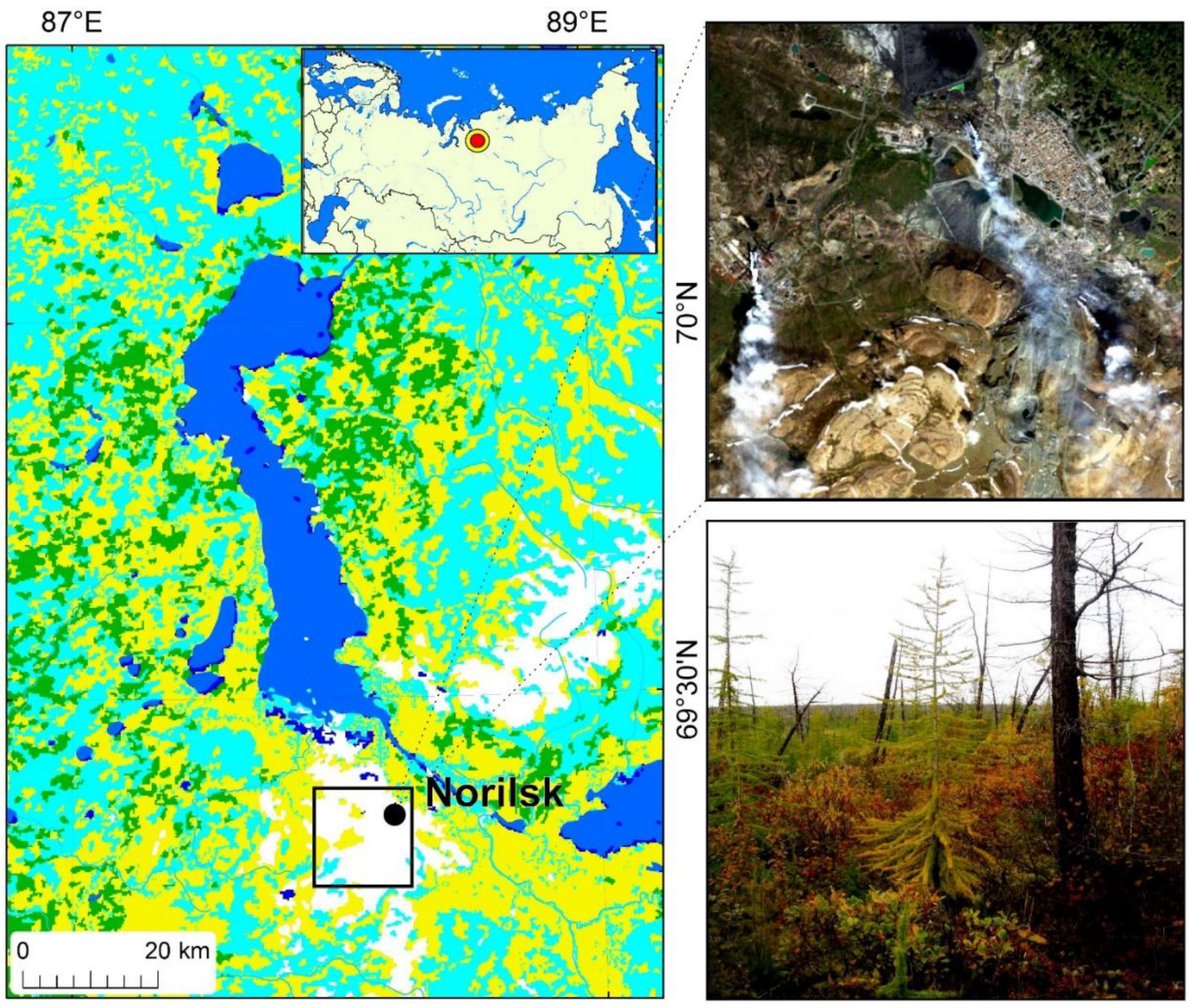
Norilsk city, one of the five most northward world cities, is located 300 km beyond the Polar Circle within the permafrost area of the Taymyr peninsula (Figure 1). Norilsk industry began in 1935 with the construction of nickel and copper plants. Firstly, concentrates of copper and nickel were obtained in 1939. Refined nickel, copper, cobalt, and platinoids production took place in 1942–1944. Since then, metallurgy and mining have rapidly continued to expand until the end of the 1980s [4]. Nadezhda, a huge third plant, started to work in 1979–1981. In 1985, Nadezhda production reached its planned volumes. Emissions from Nadezhda smelter are transferred over long distances due to high (250 m) smelter located on the plateau with elevation c. 200 m. The heights of the copper and nickel smokestacks are about 180 m and they are located in the lowlands. The Norilsk industry’s maximal production reached its maxima in 1989. However, in 1991, production decreased twice with minimum values in 1993. Nowadays, Norilsk industry provides, alongside nickel and copper, gold, silver, platinoids (palladium, osmium, iridium, rhodium, and ruthenium), selenium, tellurium, and sulfur [4].
An adverse strong by-effect of the Norilsk industry is air pollution by sulfur dioxide, nitrogen oxides, and heavy metals (Cu, Ni, Co). That caused dramatic decline and mortality of ground-cover vegetation (moss and lichen communities) and trees (primary larch, Larix sibirica Ledeb.) [5,6,7,8]. Thus, in 1990, larch decline and dieback were observed at the distances of 200 km and 80–100 km in the southwest direction from the Norilsk, respectively [9,10]. Alongside air pollutions, the recent release of c. 20,000 tons of diesel oil occurred in May of 2020 [11]. The spill impact on the water terrestrial biota was a subject of recent studies [12].
We hypothesize that current climate change might mitigate adverse pollution influence on the trees and shrubs growth.
The purpose of this study is an analysis of trees growth response to the combined influence of air pollution (SO2 emissions) and climate change on the trees growing in arctic wetlands. In addition, we studied the influence of the diesel oil spill on the tree growth.
We seek the answers to the following questions:
- -
- What was the impact of SO2 emissions on the larch (Larix sibirica Ledeb.) trees and shrubs’ (Salix spp. and alder, Duschekia fruticosa) growth?
- -
- How has climate warming influenced larch trees and shrubs’ growth?
- -
- What are the temporal trends of the gross (GPP) and net (NPP) primary production and vegetation index NDVI (Normalized Difference Vegetation Index) within the zone of pollution influence?
2. Materials and Methods
2.1. Study Area
The study domain is located within the northern wetlands, surrounded by offshoots of the Putorana plateau (Figure 1). This is the zone of continuous permafrost with multiple lakes. Sparse and open forests formed by larch, spruce (Picea obovata Ledeb.), and birch (Betula spp.). Bushes are presented mostly by willows (Salix spp.), alder (Duschekia fruticosa Pouzar), and Betula spp. Stony tundra is occupied by lichens, moss bushes, swamp ledum, and alder communities. The climate is sharply continental, with below zero (−9 ÷ −10 °C) annual air temperature (recorded minimum was −57 °C).
2.2. Field Studies
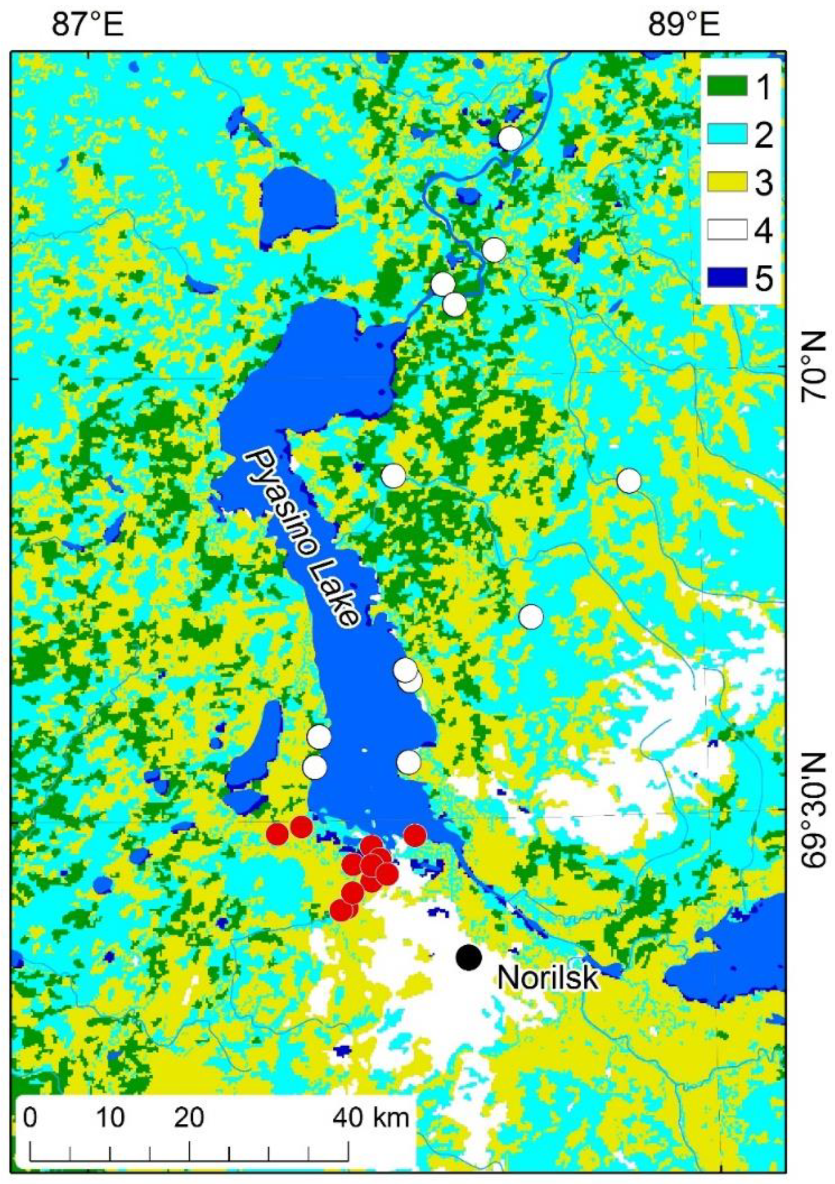
Over 2021–2022, we made a field survey within the area with heavily damaged forests (“impact zone”) and background (control) territories. Twenty-five temporary test plots (TP; approximately 0.5 ha each one) were established around the Pyasino Lake (13 and 12 TP within impact and control zones, respectively; Figure 2). Tree and stand characteristics (stem diameter, tree height, stand density, regeneration number, ground cover, and soil type) were determined. For dendrochronological analysis, we randomly selected trees within each TP. We extracted individual tree cores (small, pencil-sized pieces of wood oriented from bark to stem center perpendicular to the tree’s stem) with an increment borer from about 20 trees to represent each TP. Cores were taken at DBH height (1.3 m above ground-line) or lower (to root collar) from the stem. In the analysis we used 228 larch cores (195 survived and 33 dead trees), 19 alder cores, 59 cores of willow species from the impact zone, and 169 larch cores from the control zone.
2.3. Dendrochronological Analysis
Tree cores were mounted on wooden backing. Cores and disks were finely sanded and treated with contrast powder to enhance visualization of ring boundaries. The measurements were carried out on a LINTAB-6 platform with an accuracy of 0.01 mm. The cross-dating quality was assessed by COFECHA software (https://www.ldeo.columbia.edu/tree-ring-laboratory/resources/software; [13] (accessed on 1 December 2022)). From the measured series, we constructed a growth index (GI) chronology for each TP from raw tree-ring width in mm to unitless GI values by a detrending method with program ARSTAN ([14]; https://www.ldeo.columbia.edu/tree-ring-laboratory/resources/software (accessed on 1 December 2022)). We removed low frequency trends by fitting tree-ring series with a negative exponential curve or line with a negative slope. For statistical analysis, the GI chronology was normalized by conversion to Z-scores with a mean of zero and standard deviation of 1.0.
2.4. Eco-Climate Variables
Tree GI was analyzed against the pollution (SO2) emissions, monthly air and soil temperatures, precipitation, SPEI drought index (standardized precipitation-evapotranspiration index), soil moisture (volumetric soil water layer depth until to 7 cm), and EWTA (equivalent water thickness anomalies, or terrestrial water storage). Air temperature, precipitation, and soil moisture were obtained from ERA-5 database (https://cds.climate.copernicus.eu/cdsapp#!/dataset/reanalysis-era5-land-monthly-means?tab=overview, accessed on 15 October 2022; spatial resolution 0.1° × 0.1° [15]).
Drought index SPEI is the difference between precipitation and potential evapotranspiration [16]. Decreased SPEI indicated increased drought severity. We calculated SPEI based on ERA5-Land data by R-script (https://github.com/sbegueria/SPEI (accessed on 1 December 2022)). SO2 emissions were obtained from scientific literature and official reports [5,17,18].
The EWTA is the product of gravimetric measurements made by the GRACE satellite with on-ground resolution 1° × 1° [19]. This is characteristic of the moisture regime and represents total terrestrial water storage. EWTA data were obtained from NASA-JPL database (https://podaac-opendap.jpl.nasa.gov/opendap/hyrax/allData/tellus/L3, accessed on 15 October 2022).
GPP data (C, kg/ha) were obtained from the Terra/MODIS product MOD17A2H version 6.0 (https://lpdaac.usgs.gov/products/mod17a2hv006/, accessed on 15 October 2022). Data temporal and spatial resolutions were 8 days and 500 m, correspondingly [20]. Mosaics of GPP (as well as NPP and NDVI) composites were compiled based on median values from 8-day composites over summer periods. NPP annual values were obtained from the Terra/MODIS product MOD17A3HGF version 6.0 (https://lpdaac.usgs.gov/products/mod17a3hgfv006/, accessed on 15 October 2022). The database contained annual NPP values with a spatial resolution of 500 m [21]. NDVI were calculated based on data from the Terra/MODIS products MOD09Q1 и MOD09A1 version 6.1 (https://lpdaac.usgs.gov/products/mod09q1v006/ [22], accessed on 15 October 2022 and https://lpdaac.usgs.gov/products/mod09a1v006 [23], accessed on 15 October 2022; spatial resolution 250 m).
Wind rise was generated based on wind direction hourly data that were obtained from the nearest of the Norilsk stations (station 23077 and 23078; coordinates 69.33° N/87.95° E and 69.33° N 88.25° E, correspondingly).
2.5. Method of Groundcover Mapping
The created land-cover classification was based on the analysis of MODIS summer scenes obtained in 2022. Seven MODIS spectral bands were used. Bands 3–7 were resampled from 453 m spatial resolution to 231 m using the non-linear downscaling algorithm [24,25]. We used the Support Vector Machine classification method [26]. Training samples were generated based on the ground data, high-resolution scenes and aero-photography, and topographic maps. The accuracy of the classification map was estimated using the error matrix and kappa statistics [27]. The overall accuracy of the classification is 92% (kappa = 0.88). Further land-cover classes along the river valleys were identified based on the GMTED digital elevation model (https://www.usgs.gov/core-science-systems/eros/coastal-changes-and-impacts/gmted2010, accessed on 15 October 2022) and the dataset of water bodies Global Water Surface Extent [28]. The spatial resolution of the created map is ~250 m, corresponding to medium-scale maps of M 1:500,000 [29].
2.6. Statistical Analysis
Four sets of statistical analysis were applied to the GI and environmental variables. Pearson correlation analysis identified significant relationships between the GI and individual climate variables. Spearman’s correlation coefficient was used to identify the relationship between GI and sulfur dioxide values. The piecewise (also known as segmented or broken-stick) regression analysis was used to detect breakpoints in the time-series of larch GI, GPP, and NPP [30]. We used StatSoft Statistica (http://statsoft.ru (accessed on 1 December 2022)) and IBM SPSS Statistics Base V27 (https://www.ibm.com/analytics/spss-statistics-software (accessed on 1 December 2022)) software for statistical analysis.
We used the Theil–Sen regression to determine tendencies (trends) in dynamics of NDVI, GPP, NPP, and climate. The Theil–Sen estimator is a non-parametric method for fitting a line to sample points in the plane by choosing the median of the slopes of all lines through pairs of points and it is based on the Kendall tau correlation coefficient [31,32]. This estimator is less sensitive to outliers, and it is more accurate than the simple linear regression [33]. We used the Theil–Sen estimator realized in the Python library pymannkendall 1.4.2 (https://pypi.org/project/pymannkendall (accessed on 1 December 2022)). The source code of the pymannkendall was adopted to Python 2.7 and used in the ESRI ArcGIS software to apply it to analyze multiband raster datasets represented by time-series of NDVI, GPP, NPP, and climate variables for 2000–2021. As a result, raster datasets of regression slopes and p-values were determined. Additionally, for NDVI, GPP, and NPP, a floating starting year (2001–2017) of the most significant trends were calculated with the last year, fixed, and equal to 2021.
3. Results
3.1. Tree and Test Plot Characteristics
Tree species are represented by Larix sibirica, Picea obovata, and Betula sp. Larch the dominating tree species in the region. Larch tree characteristics varied, including mean tree height (6–10 m), DBH (diameter at breast height, i.e., 1.3 m) (13–16 cm), and age (15–435 years at DBH height; median age 95 years). The shrub layer was composed of alder, willow, and birch (Duschekia fruticose, Salix spp. and Betula spp.). The low shrubs and herbaceous ground cover layer contained Ledum palustre L., Vaccinium vitis-idaea L., Vaccinium uliginosum L., Carex spp., and Equisetum arvense L.
3.2. Climate Variables
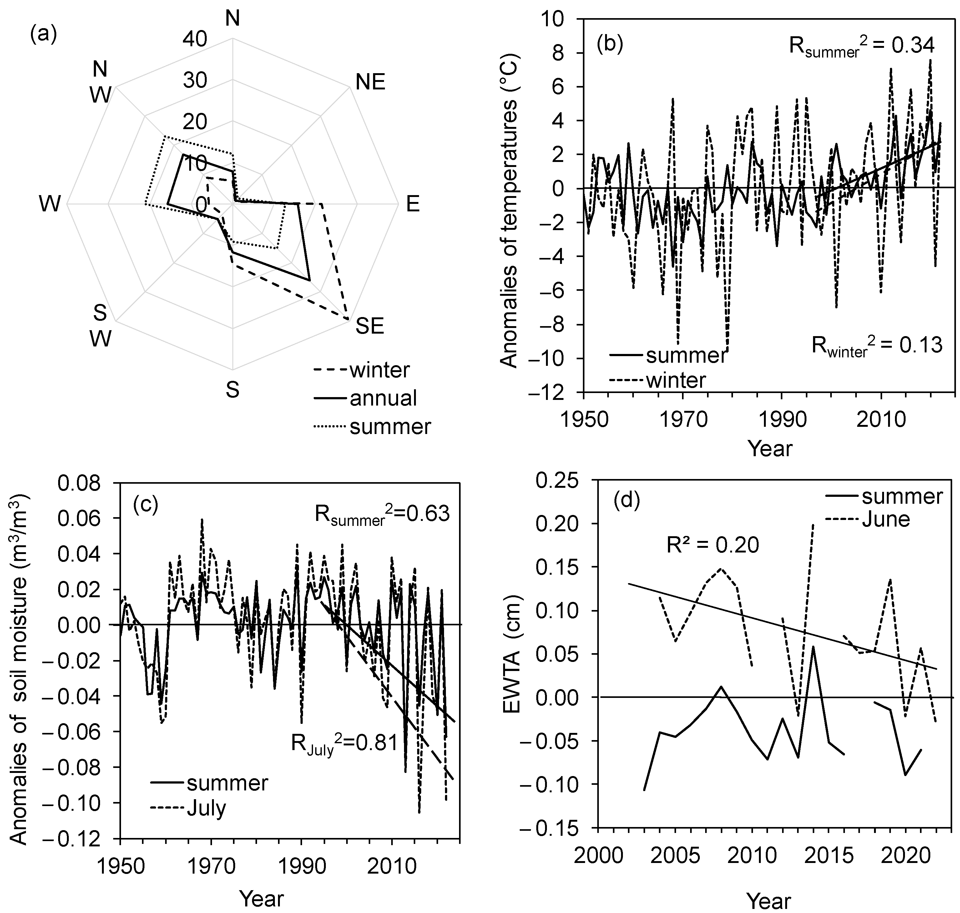
Within the study area, northwest winds prevailed during the summer and southeast ones prevailed in winter (Figure 3a). Summer and winter air temperatures have been increasing since 1990 (R2 = 0.13–0.34; Figure 3b). Soil summer moisture has been decreasing since 2000 (R2 = 0.63; Figure 3c). A strong decreasing trend experienced minimal values soil moisture in July, which indicated an acute drought frequency increase (R2 = 0.81; Figure 3c). Terrestrial moisture content (GRACE-derived June values) has been decreasing since 2000 (R2 = 0.20; Figure 3d). Meanwhile, precipitation values have stagnated.
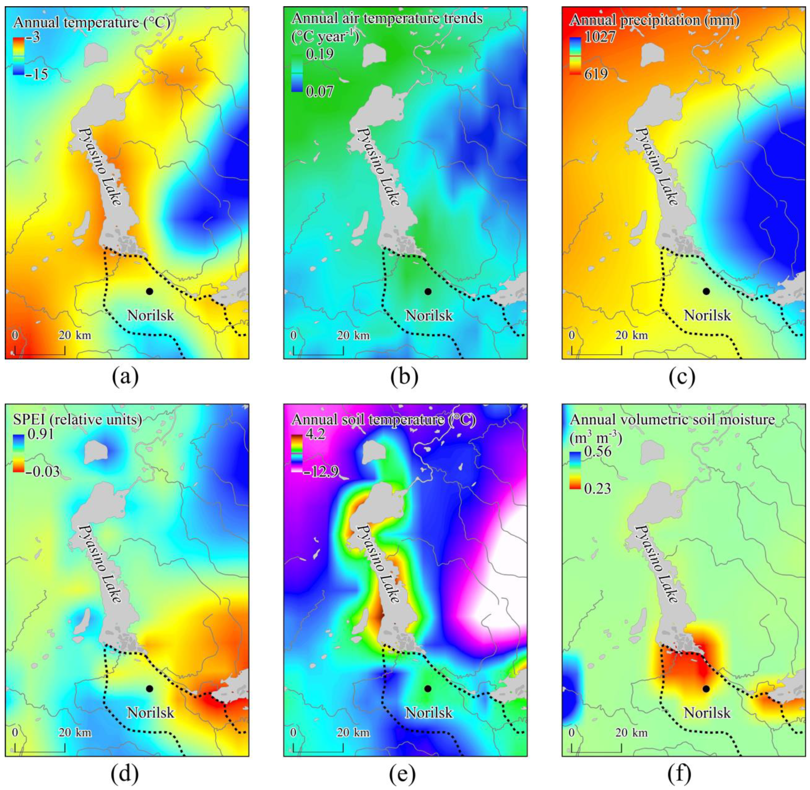
Maps of eco-climate variables within the study area show their spatial distribution within the study area (Figure 4). The annual temperature varied from c. −3 °C (in wetlands) to −15 °C (in mountains). Positive temperature trends were observed on the major part of the lowlands (Figure 4a,b). Annual precipitation varied from c. 600 mm/year (wetlands) to 1000 mm/year (mountains) (Figure 4c). Maximal values of atmospheric drought (indicated by drought index SPEI) were observed in the area southeast of Norilsk (Figure 4d). The highest soil temperatures are located around the Pyasino Lake and southeast of Norilsk (Figure 4e). Minimal soil moisture content was observed southward of Pyasino Lake (Figure 4f).
3.3. Pollution Sources and Emissions Transfer
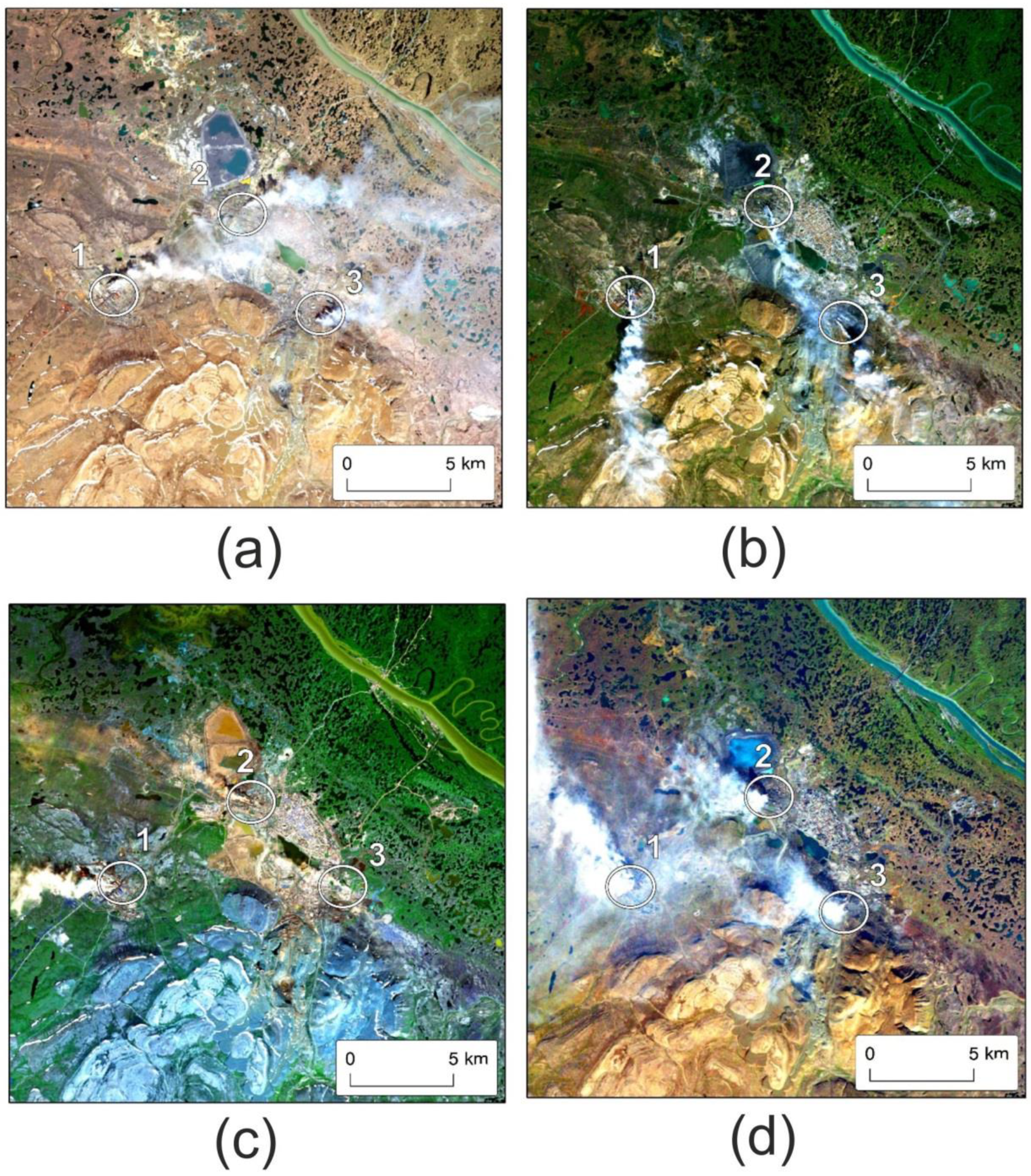
The locations of pollution sources (Nadezhda, copper, and nickel plants) are presented in Figure 5. Pollution transfer is controlled by wind direction and speed and terrain topography. Although the main directions of pollution transfer (according to wind rose, Figure 3a) are southeast and northwest (Figure 5b), pollution might be transferred to the other directions (Figure 5a,c) or stay mostly within smelters location in the case of anticyclone-caused still weather (Figure 5d). Under certain metrological conditions, part of the sulfur dioxide emissions extends to the middle and northern parts of the territories adjacent to Lake Pyasino. However, no significant effect of SO2 emissions on the radial increment of larch trees growing in this area was found.
3.4. Trees’ Growth Index Responses to Pollution Impact and Climate Variables
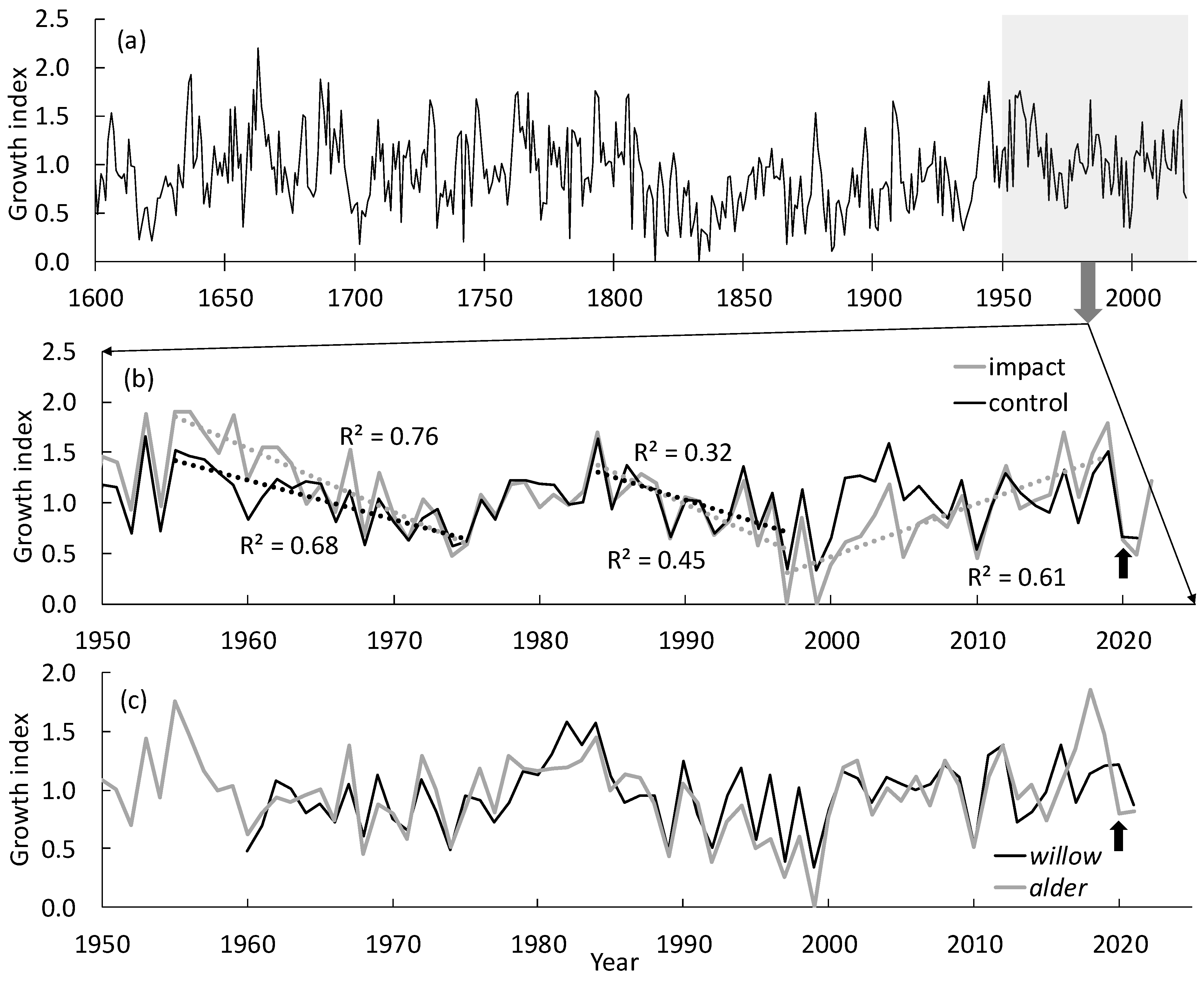
The dynamics of larch growth index (GI) in the impact and control zones until 1950 was highly synchronous (correlation coefficient r = 0.9; Figure 6). In the second half of the 20th century, that synchronicity decreased (r = 0.79) due to changes mainly in the low-frequency component. Since 2000, a GI increase has been recorded for trees in the impact zone mostly, and during the last decade (compared to the same pre-warming period of 1990–1999) larch GI increased by 1.6 times; for comparison, within the control zone, GI increased 1.2 times (Figure 6b).
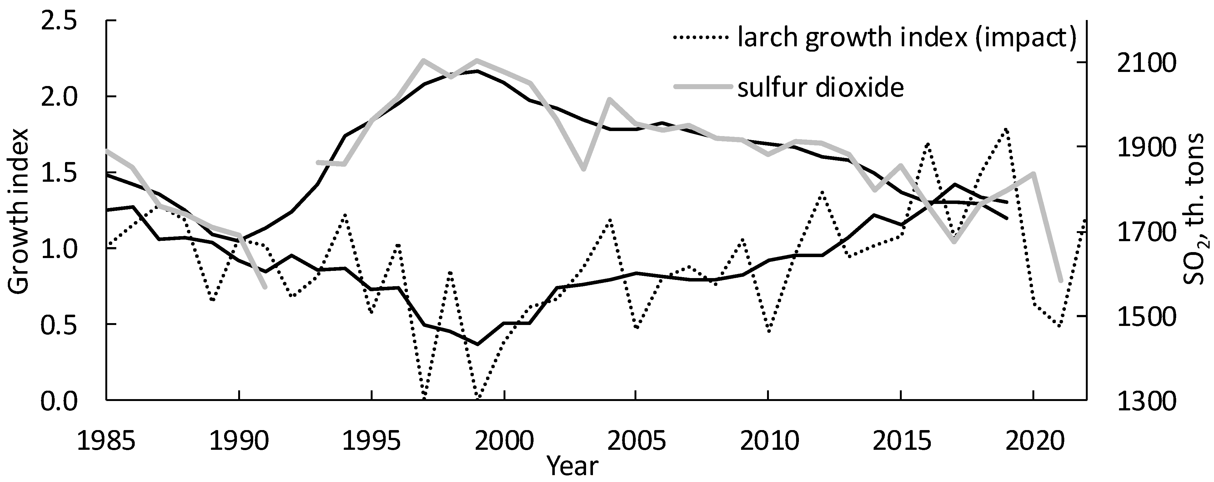
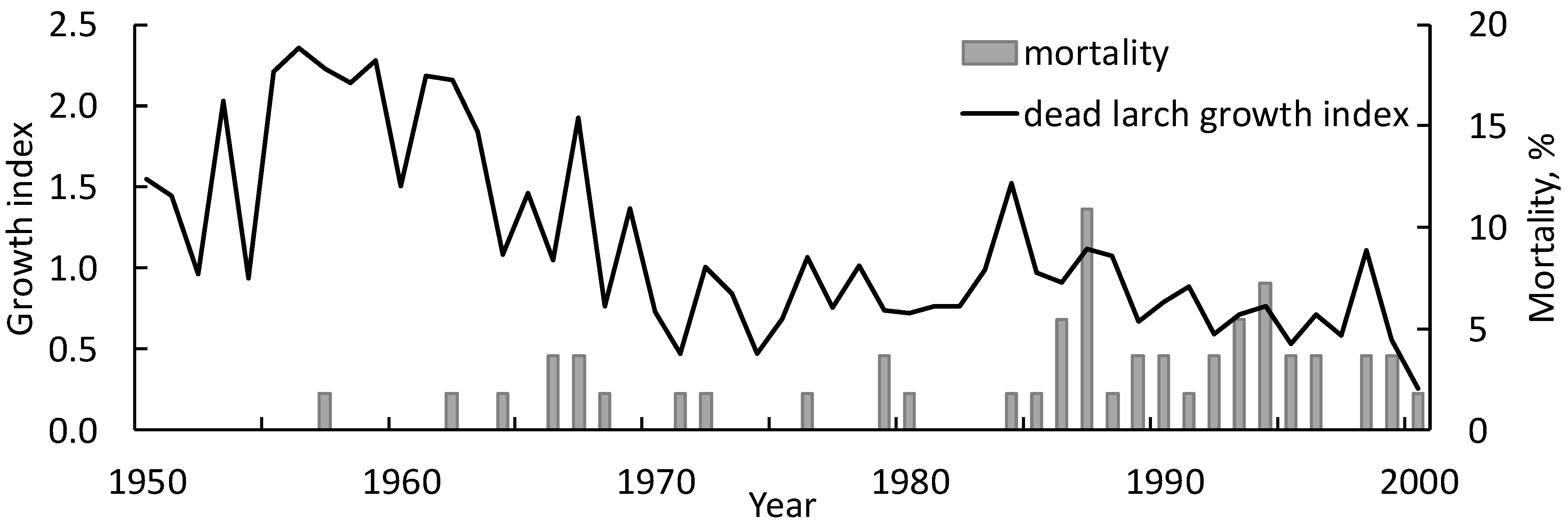
The dynamics of radial increment (a decrease in GI until the second half of the 1990s with a subsequent increase at the beginning of the 21st century) and the dynamics of SO2 emissions are in antiphase (an increase and subsequent decrease in emissions; Figure 7). Although the local minima of the radial increment during this period correspond to similar minima recorded for other wood species and are likely to be of a climatic origin, the increase in the radial increment in the impact zone (low frequency component; Figure 6b,c) coincides in time with a decrease in SO2 emissions. According to dendrochronological analysis, the onset of tree mortality dates back to the late 1950s. The maximum mortality of larch trees was observed in 1980–1990 against the background of an increase in sulfur dioxide emissions (Figure 8).
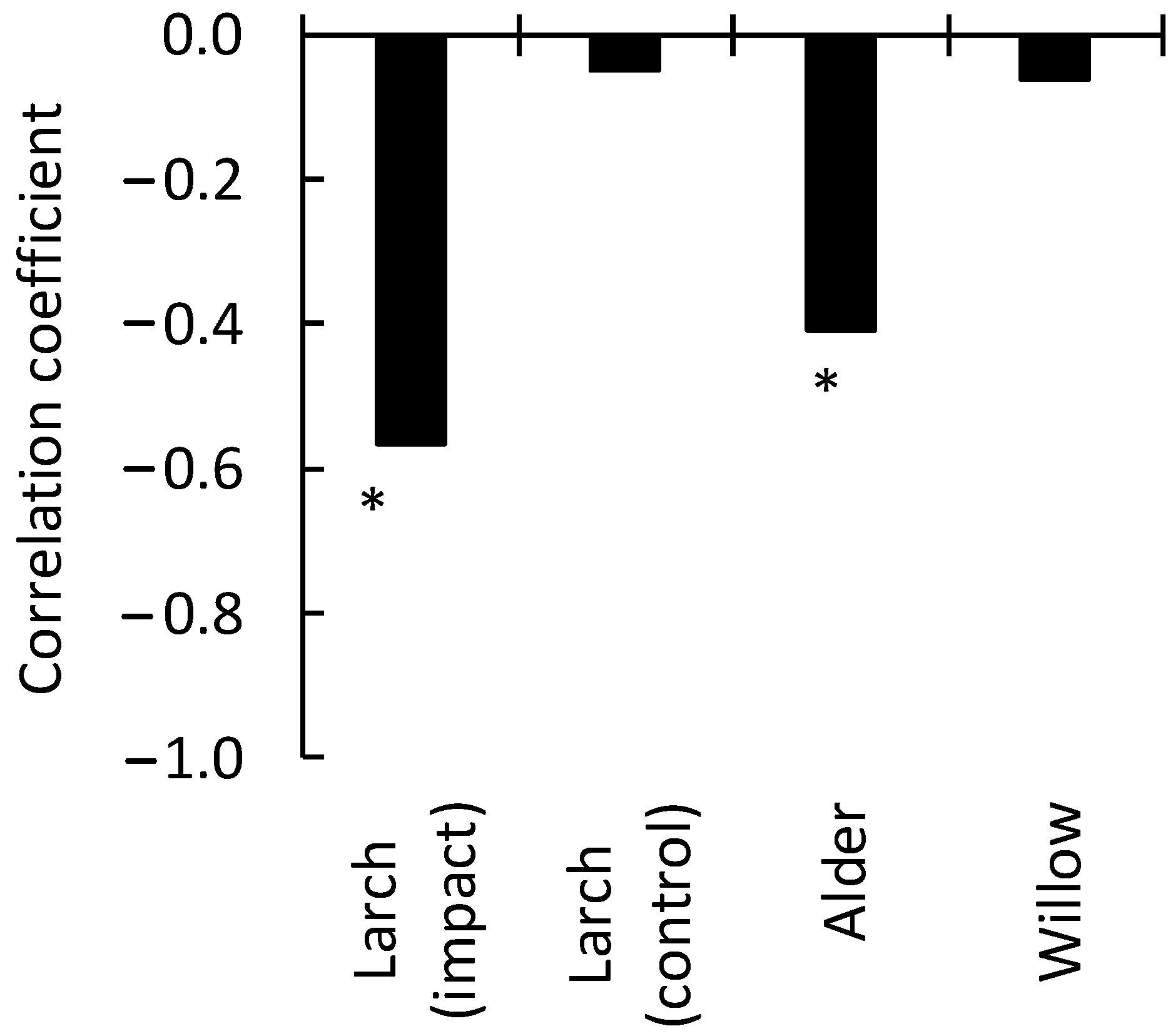
Comparative analysis of the GI and sulfur dioxide emissions dynamics for the period 1985–2020 (i.e., for period of reliable SO2 emissions data) indicates significant dependence of GI on emissions (r = −0.56 for larch and r = −0.41 for alder, p < 0.05; Figure 9). No significant correlations between GI and sulfur dioxide emissions were found for the larch trees in the control zone and for the willow in the impact zone.
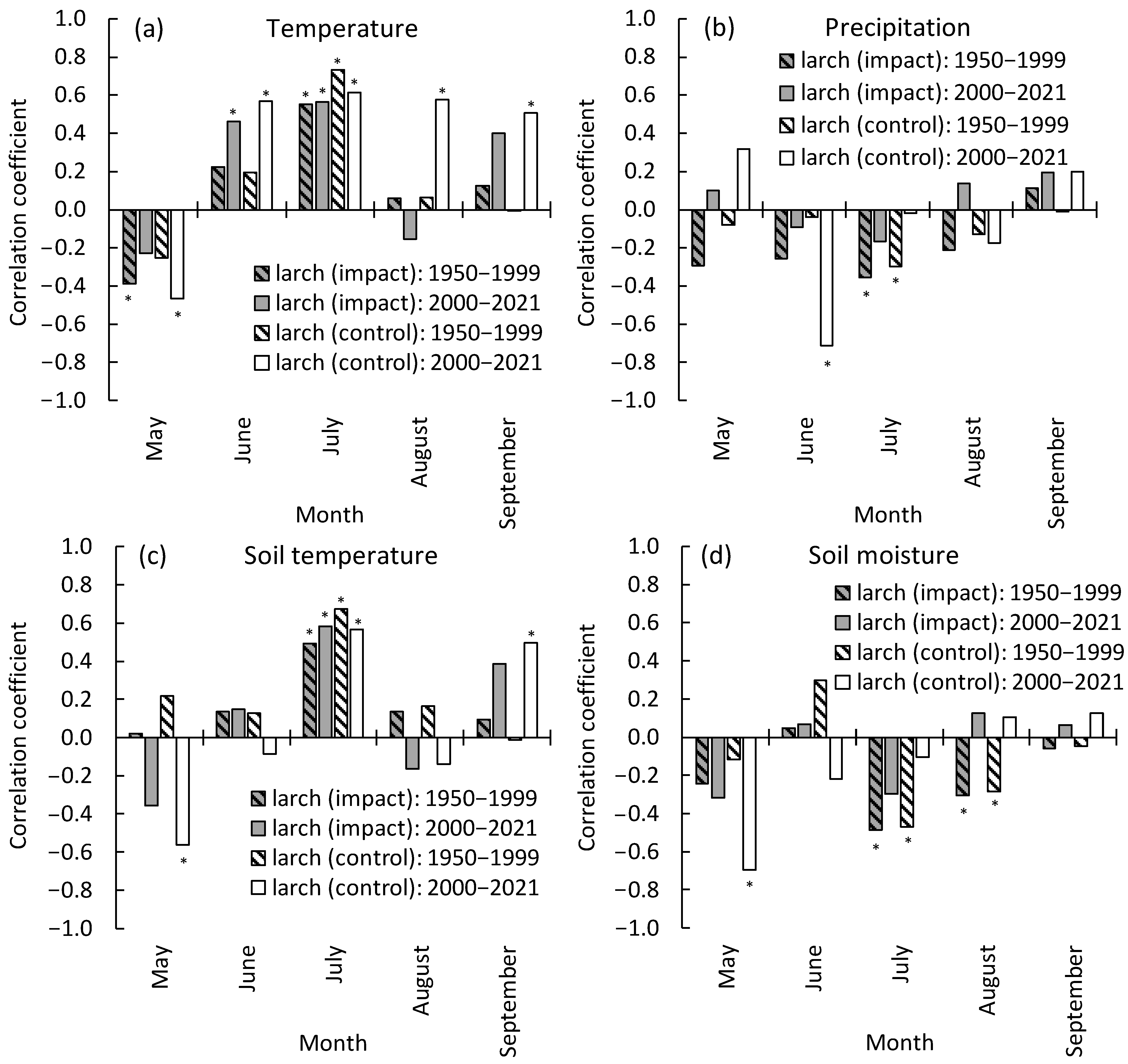
Correlation analysis revealed significant stimulating effects of the air temperature increase in July and inhibition effects of precipitation (July–August) and soil moisture on trees’ GI (Figure 10). There are no significant differences in the reaction of trees’ GI on climatic changes between the impact and control zones. It should be noted that the observed prolongation of the growth period, due to increased temperature in June and September, stimulates radial growth increase. Meanwhile, there is significant negative correlation between GI and the spring warmth (temperature increases in May; Figure 10a).
The multiple regression analysis indicates the volume of SO2 emissions and air temperature as the main factors influencing the radial increment of larch trees in the impact zone. At the same time, the air temperature in June–July has a stimulating effect on radial increment, and the May temperature has an inhibitory effect (Equation (1)).
where GI—growth index, TJJ—June–July temperature, TMAY—May temperature, SO2—values of SO2 emissions. Explained dispersion: R2 = 0.7. Period: 1985–2020.
GI = 0.65 × TJJ − 0.43 × SO2 − 0.35 × TMAY − 0.04,
In the control, the radial increment does not depend on sulfur dioxide emissions and is determined by air temperature and soil moisture (“cold soils effect”; Equation (2)):
where GI—growth index, TJJ—June–July temperature, PJUNE—June precipitation, SMMAY—soil moisture. Explained dispersion: R2 = 0.55. Period: 1985–2020.
GI = 0.04 + 0.47 × TJJ − 0.38 × PJUNE − 0.31 × SMMAY,
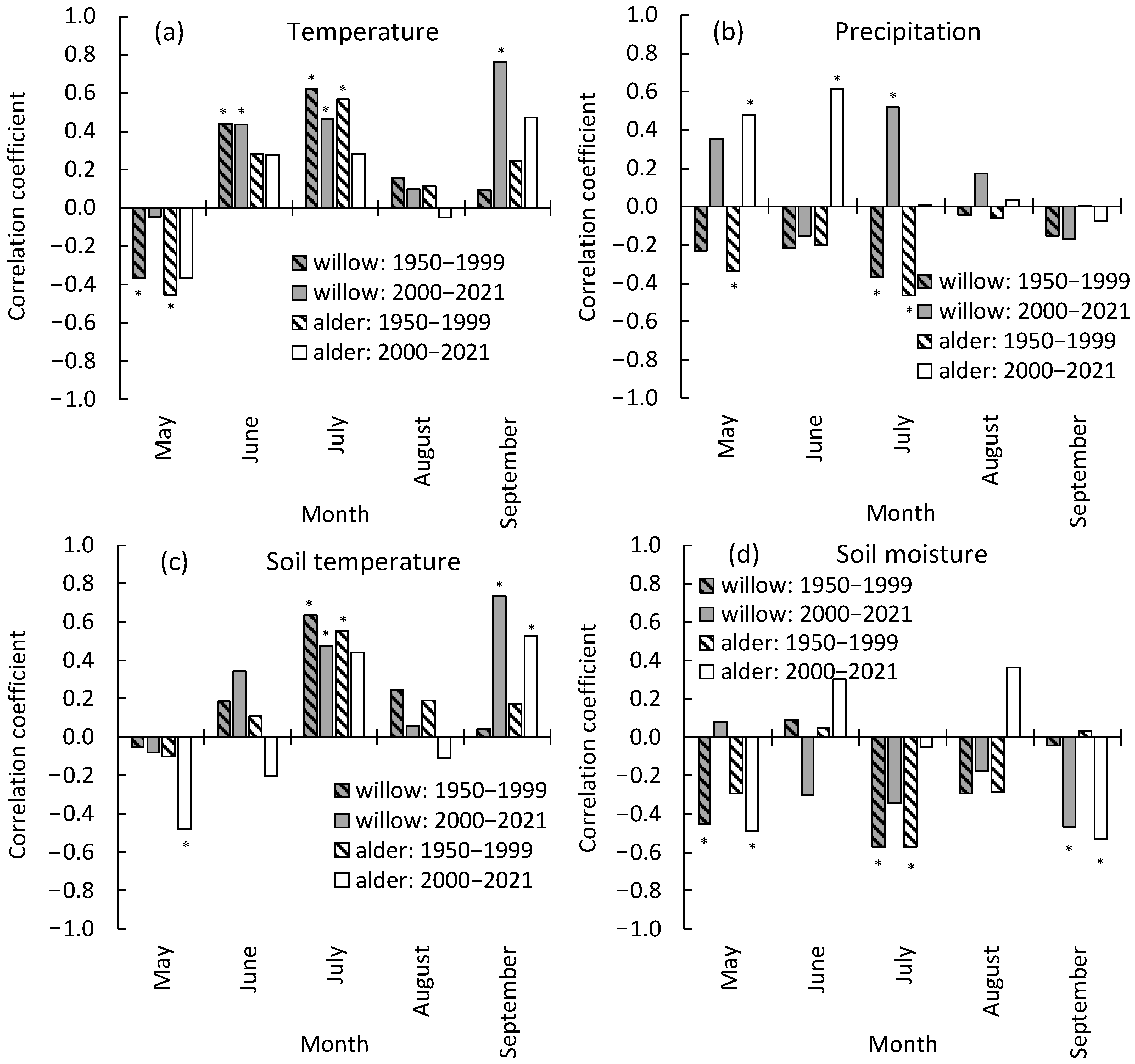
Shrub species (willow and alder) also have a positive response to climate warming (Figure 11). In addition to significant positive correlations with July temperature, the growing season is prolongation indicated by positive correlations with September and June temperatures. As in the case of larch, negative correlations with May temperatures are observed. Similar to larch, an inhibitory effect of excessive soil moisture on radial increment is also observed for bushes (Figure 11d).
3.5. GPP, NPP, and NDVI Dynamics
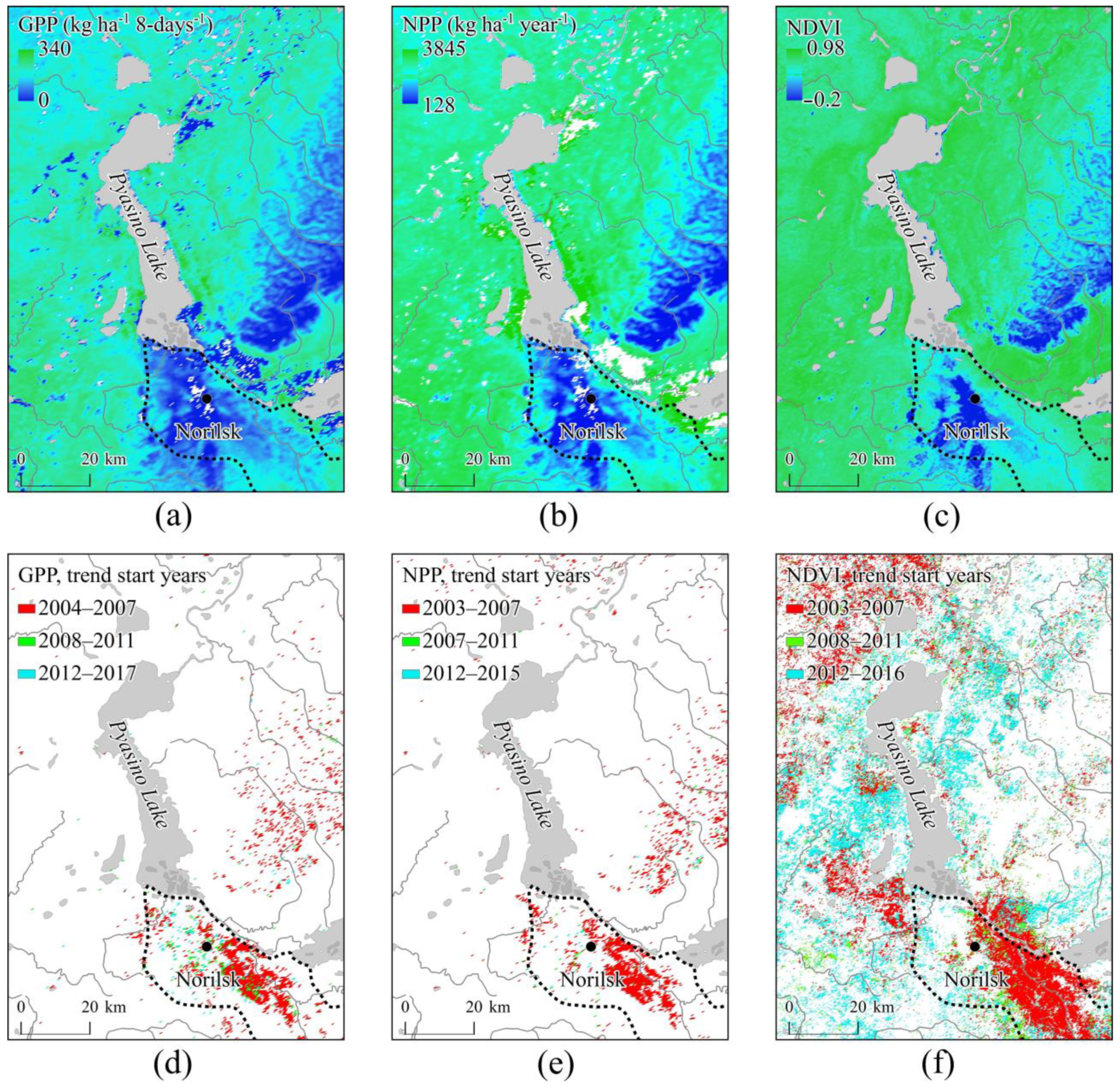
GPP, NPP, and NDVI maps indicated the minimal values of GPP, NPP, and NDVI in the areas of the main air pollution impact (Figure 12a–c). Meanwhile, in the areas where increasing trends of vegetation productivity were observed (although in the most affected zone (westward from Norilsk), trends were mostly zero (Figure 12d–f). The start of the positive trends dated mostly to 2003–2005 (Figure 12d–f).
4. Discussion
Norilsk industry emissions caused the biggest large-scale decline and mortality of forests beyond the Arctic circle. Tree growth in the studied northern wetlands was influenced by both air emissions (SO2 mostly) and the warming climate. The beginning of industrial emissions referred to the end of 1930, whereas significant “emissions-growth index” correlations has been observed since 1950. The latter coincided with the first reported larch forests’ decline and mortality [9]. The growth decrease was continuous until the end of 1990, when the tree mortality rate reached its maxima. In the following period (since 2000), larch growth experienced an increase, which was attributed to the combined effect of pollution load decrease and air and soil warming. SO2 emissions (the main pollutant) decreased from c. 2.5 M t/year in 1980 to c. 1.6 M t/year at present due to technology improvements, together with nickel plant closure (2016). Some contribution to the growth positive trends may be related to the CO2 fertilization effect. However, that effect is low in cold habitats [34]. In the “background zone”, the larch growth increase correlated with air temperature only, although certain wind directions emissions partly covered that area, which indicated that emissions load was within the larch compensatory range.
Since the end of 1990, elevated air temperatures in the beginning (June) and in the end (August–September) stimulated larch growth, whereas July temperatures’ influence on the growth decreased. For comparison, during the previous period (1950–2000), larch GI was mostly dependent on the July temperatures (R2 = 0.54), whereas June and August–September influences were insignificant. A similar effect of low growth response to July temperature was described for the Siberian pine growth within mountain forest-tundra ecotone [35]. Thus, with warming larch growth limitation by July, temperatures shifted to temperatures in the beginning and the end of growth period. Meanwhile, early (May) warms led to a GI decrease. That effect was caused by “warming provocation” of the phloem and cambium activity, while soil water was not still available with consequent needles and twigs desiccation, as well as the damage by late frosts. In extreme cases, larches may flash needles prior to snowmelt.
Opposite to temperature, soil moisture increases negatively influenced larch growth due to the “cold soils effect”, i.e., low soil temperatures slow down root activity with consequent tree growth decreases (Figure 10d and Figure 11d). This effect is most pronounced in waterlogged habitats. The other negative factor is a limited root oxygen supply within poorly drained soils. However, growth limitation by water availability has also been described in permafrost zones [36,37,38]. Larch may experience a moisture deficit at the beginning of the growth period when elevated air temperatures are sufficient for photosynthesis, while soils are still mostly frozen [37].
For bushes (willow and alder), we observed similar larch growth and temperature shifts. Notably, that GI of willow more strongly responded to the June and September temperatures in comparison with larch and alder. That effect may be caused by non-leaf photosynthesis, i.e., photosynthesis occurred in the bark tissues. For example, for aspen, which also belongs to the Salicaceae family, non-leaf (bark) photosynthesis produced 15–20% of the total photosynthetic production [39]. In a harsh environment, willow species may grow even in the leafless form. Meanwhile, the significance of non-leaf photosynthesis for shrubs and trees surviving in the harsh habitat needs further studies. Notably, the growth index of Salix species did not significantly correlate with SO2 emissions, even within the zone of strong emissions impact that indicates a high resistance of these species to SO2 influence. Thus, willow species may be used for reclamation of the polluted territories.
Alongside tree growth increase, increasing trends of vegetation indexes (GPP, NPP, and NDVI) were observed in part of the wetland. Interestingly, the high increase was located mainly within the area of larch trees mortality that occurred during 1960–1990. Vegetation productivity increase was located mostly within areas with lower soil water content, whereas in wetlands with high moisture content (the majority of the background territories), GPP and NPP trends were mostly insignificant. The beginning of those trends is dated mostly by 2003–2005 and is associated with emissions decrease, warming, and invasion and growth of resistant species (birch, willow and other bushes, and graminoids). As noted by [40], the main direction of the phytocenosis successions is the substitution of the forests and moss–lichen associations to the grass and bushes communities. An additional factor of polluted area greening is warming-driven larch growth increase. Although [8] reported zero larch regeneration within the area of total larch mortality, we observed a minor amount of larch seedling in the area of former tree mortality. Certainly, regeneration establishment and, more generally, species composition is a dynamic process that needs further study.
Alongside the above-discussed factors, pollution-origin nitrogen fertilization may also promote positive trends in vegetation productivity. Annual Norilsk NOx emissions varied within 9–25 thousand tons/year. Studies of pollution-caused nitrogen fertilization indicated an increase of tree growth (e.g., [41,42]).
Finally, we found that dispel fuel spill’s influence (which occurred in 2020) on the tree species was insignificant. Meanwhile, all moss species and some vascular ones are highly intolerant to petroleum pollution, whereas aquatic and riverside grasses are petroleum-resistant [12].
5. Conclusions
Sulfur dioxide emissions, air temperature, soil moisture, and temperature are the main constraints of the larch growth in the studied northern wetlands. SO2 influence led to larch growth decrease from 1950 until the end of 1990 when tree mortality reached its maxima. Since 2000, larch growth has been increasing due to combined effect of air pollution decrease and climate warming. With warming, larch and bushes growth limitation by July temperatures switch to the temperatures in the beginning of the growth period. Meanwhile, early spring warmth led to GI decrease due to “metabolism provocation” while soil water was not available. In some years, even “larch trees greening” phenomenon occurred while the background was still snow-covered. Consequently, this caused twigs and needles desiccation, together with damage by the late frosts.
During recent decades, increasing trends of GPP, NPP, and NDVI were also observed on parts of the wetland. Notably, high productivity trends were located partly in the zone of former trees’ mortality. Positive trends were associated with emissions volume decrease, climate warming, invasion of resistant species (willows, graminoids, bushes, and birch), and increased larch tree growth. In addition, soil fertilization due to NOx emissions may potentially stimulate vegetation productivity increase. Finally, we found that the fuel spill that happened in 2020 had no influence on the larch, whereas some aquatic species (mosses mostly) were damaged.
Author Contributions
Conceptualization, V.I.K.; Methodology, V.I.K. and I.A.P.; Validation, V.I.K., S.T.I. and I.A.P.; Formal Analysis, S.T.I., I.A.P., M.L.D. and A.S.G.; Investigation, V.I.K., S.T.I. and I.A.P.; Resources, S.T.I., A.S.S., M.L.D. and A.S.G.; Data Curation, S.T.I., I.A.P. and A.S.G.; Writing—Original Draft Preparation, V.I.K.; Visualization, S.T.I., M.L.D., A.S.G. and A.S.S.; Supervision, V.I.K.; Project Administration, V.I.K.; Funding Acquisition, V.I.K. All authors have read and agreed to the published version of the manuscript.
Funding
The research was funded by the Tomsk State University Development Program («Priority-2030») and contract NTEK-32-523-1/21 for the project of restoration work to compensate for damage to wildlife, as well as other environmental components affected by the accidental oil spill.
Data Availability Statement
The data presented in this study are openly available: climate data in https://cds.climate.copernicus.eu (accessed on 15 October 2022) reference number [15]; SPEI in http://sac.csic.es/spei (accessed on 15 October 2022) reference number [15]; EWTA in https://podaac-opendap.jpl.nasa.gov/opendap/hyrax/allData/tellus/L3 (accessed on 15 October 2022), reference number [18]; GPP in https://lpdaac.usgs.gov/products/mod17a2hv006 (accessed on 15 October 2022), reference number [19]; NPP in https://lpdaac.usgs.gov/products/mod17a3hgfv006/ (accessed on 15 October 2022) reference number [20]; NDVI in https://lpdaac.usgs.gov/products/mod09q1v006/ accessed on 15 October 2022 reference number [22] and https://lpdaac.usgs.gov/products/mod09a1v006 (accessed on 15 October 2022) reference number [23]; Land-cover in https://www.usgs.gov/core-science-systems/eros/coastal-changes-and-impacts/gmted2010 (accessed on 15 October 2022) reference number [28].
Conflicts of Interest
The authors declare no conflict of interest.
References
- Chylek, P.; Folland, C.; Klett, J.D.; Wang, M.; Hengartner, N.; Lesins, G.; Dubey, M.K. Annual Mean Arctic Amplification 1970–2020: Observed and Simulated by CMIP6 Climate Models. Geophys. Res. Lett. 2022, 49, e2022GL099371. [Google Scholar] [CrossRef]
- Mack, M.C.; Walker, X.J.; Johnstone, J.F.; Alexander, H.D.; Melvin, A.M.; Jean, M.; Miller, S.N. Carbon loss from 650 boreal forest wildfires offset by increased dominance of deciduous trees. Science 2021, 372, 280–283. [Google Scholar] [CrossRef]
- Kharuk, V.I.; Dvinskaya, M.L.; Im, S.T.; Golyukov, A.S.; Smith, K.T. Wildfires in the Siberian Arctic. Fire 2022, 5, 106. [Google Scholar] [CrossRef]
- Dolgikh, V.I. Phenomenon of Norilsk: History of the Norilsk Industrial Region; Polar Star: Moscow, Russia, 2006. [Google Scholar]
- Kozlov, M.V.; Zvereva, E.L.; Zverev, V.E. Impacts of Point Polluters on Terrestrial Biota: Comparative Analysis of 18 Bontaminatedreas; Springer: Dordrecht, The Netherlands, 2009; Volume XVII, p. 466. ISBN 978-90-481-2466-4. [Google Scholar] [CrossRef]
- Korets, M.A.; Ryzhkova, V.A.; Danilova, I.V. GIS-Based approaches to the assessment of the state of terrestrial ecosystems in the Norilsk industrial region. Contemp. Probl. Ecol. 2014, 7, 643–653. [Google Scholar] [CrossRef]
- Kirdyanov, A.V.; Prokushkin, A.S.; Tabakova, M.A. Tree-ring growth of Gmelin larch under contrasting local conditions in the north of Central Siberia. Dendrochronologia 2013, 31, 114–119. [Google Scholar] [CrossRef]
- Kirdyanov, A.V.; Krusic, P.J.; Shishov, V.V.; Vaganov, E.A.; Fertikov, A.I.; Myglan, V.S.; Barinov, V.V.; Browse, J.; Esper, J.; Ilyin, V.A.; et al. Ecological and conceptual consequences of Arctic pollution. Ecol. Lett. 2020, 23, 1827–1837. [Google Scholar] [CrossRef]
- Kharouk, V.I.; Winterberger, K.; Tsibul’skii, G.M.; Yakhimovich, A.P.; Moroz, S.N. Technogenic disturbance of pretundra forests in Noril’sk Valley. Russ. J. Ecol. 1996, 27, 406–410. [Google Scholar]
- Zubareva, O.N.; Skripal’shchikova, L.N.; Greshilova, N.V.; Kharuk, V.I. Zoning of landscapes exposed to technogenic emissions from the Norilsk mining and smelting works. Russ. J. Ecol. 2003, 34, 375–380. [Google Scholar] [CrossRef]
- Norilsk Nickel Annual Reports (2011–2021). Available online: https://www.nornickel.com/investors/reports-and-results (accessed on 10 October 2022).
- Telyatnikov, M.Y. Dynamics of the Phytodiversity of Natural Ecosystems Affected by Oil Products in the Norilsk Industrial District. Contemp. Probl. Ecol. 2022, 15, 160–179. [Google Scholar] [CrossRef]
- Holmes, R.L. Computer-assisted quality control in tree-ring dating and measurement. Tree-Ring Bull. 1983, 44, 69–75. [Google Scholar]
- Cook, E.R.; Holmes, R.L. User’s Manual for Program ARSTAN. In Tree-Ring Chronologies of Western North America: California, Eastern Oregon and Northern Great Basin; Holmes, R.L., Adams, R.K., Fritts, H.C., Eds.; Chronology Series 6; Laboratory of Tree-Ring Research: Tucson, AZ, USA, 1986; pp. 50–65. [Google Scholar]
- Hersbach, H.; Rosnay, P.; Bell, B.; Schepers, D.; Simmons, A.; Soci, C.; Abdalla, S.; Alonso-Balmaseda, M.; Balsamo, G.; Bechtold, P.; et al. Operational Global Reanalysis: Progress, Future Directions and Synergies with NWP. ECMWF ERA Report Series. 2018. Available online: https://www.ecmwf.int/en/elibrary/18765-operational-global-reanalysis-progress-future-directions-and-synergies-nwp (accessed on 15 October 2022).
- Vicente-Serrano, S.M.; Beguería, S.; López-Moreno, J.I. A multiscalar drought index sensitive to global warming: The standardized precipitation evapotranspiration index. J. Clim. 2010, 23, 1696–1718. [Google Scholar] [CrossRef]
- Kharuk, V.I. Air pollution impact on subarctic forests at Norilsk, Siberia. In Forest Dynamics in Heavily Polluted Regions; Innes, J.L., Oleksyn, J., Eds.; CABI International: Wallingford, UK, 2000; pp. 77–86. [Google Scholar]
- Ministry of Ecology and Environmental Management of the Krasnoyarsk Region. The Governmental Report on the State and Protection of the Environment in Krasnoyarsk Region in 2018; Polygraph-Avanta Ltd.: Krasnoyarsk, Russia, 2018; pp. 2006–2021. [Google Scholar]
- Landerer, F.W.; Flechtner, F.M.; Save, H.; Webb, F.H.; Bandikova, T.; Bertiger, W.I.; Bettadpur, S.V.; Byun, S.H.; Dahle, C.; Dobslaw, H.; et al. Extending the global mass change data record: GRACE Follow-On instrument and science data performance. Geophys. Res. Lett. 2020, 47, e2020GL088306. [Google Scholar] [CrossRef]
- Running, S.; Mu, Q.; Zhao, M. MOD17A2H MODIS/Terra Gross Primary Productivity 8-Day L4 Global 500m SIN Grid V006; NASA EOSDIS Land Processes DAAC: Sioux Falls, SD, USA, 2015. [CrossRef]
- Running, S.; Zhao, M. MOD17A3HGF MODIS/Terra Net Primary Production Gap-Filled Yearly L4 Global 500 m SIN Grid V006; NASA EOSDIS Land Processes DAAC: Sioux Falls, SD, USA, 2019. [CrossRef]
- Vermote, E. MOD09Q1 MODIS/Terra Surface Reflectance 8-Day L3 Global 250m SIN Grid V006; NASA EOSDIS Land Processes DAAC: Sioux Falls, SD, USA, 2015.
- Vermote, E. MOD09A1 MODIS/Terra Surface Reflectance 8-Day L3 Global 500m SIN Grid V006; NASA EOSDIS Land Processes DAAC: Sioux Falls, SD, USA, 2015.
- Trishchenko, A.P.; Luo, Y.; Khlopenkov, K.V. A method for downscaling MODIS land channels to 250-m spatial resolution using adaptive regression and normalization. Remote sensing for environmental monitoring, GIS applications, and geology. Proc. SPIE 6366 2006, VI, 636607. [Google Scholar] [CrossRef]
- Che, X.; Feng, M.; Jiang, H.; Song, J.; Jia, B. Downscaling MODIS surface reflectance to improve water body extraction. Adv. Meteorol. 2015, 2015, 424291. [Google Scholar] [CrossRef] [Green Version]
- Burges, C.J. A Tutorial on support vector machines for pattern recognition. Data Min. Knowl. Discov. 1998, 2, 121–167. [Google Scholar] [CrossRef]
- Russell, G.; Congalton, K.G. Assessing the Accuracy of Remotely Sensed Data Principles and Practices, 3rd ed.; CRC Press: Boca Raton, FL, USA, 2020; p. 348. ISBN 9780367656676. [Google Scholar]
- Pekel, J.F.; Cottam, A.; Gorelick, N. High-resolution mapping of global surface water and its long-term changes. Nature 2016, 540, 418–422. [Google Scholar] [CrossRef]
- Tobler, W. Measuring spatial resolution. In Proceedings of the Land Resources Information Systems Conference, Beijing, China; 1987; pp. 12–16. [Google Scholar]
- Ryan, S.E.; Porth, L.S. A Tutorial on the Piecewise Regression Approach Applied to Bedload Transport Data; Gen. Tech. Rep. RMRS-GTR-189; Department of Agriculture, Forest Service, Rocky Mountain Research Station: Fort Collins, CO, USA, 2007; p. 41.
- Sen, P.K. Estimates of the regression coefficient based on Kendall’s tau. J. Am. Stat. Assoc. 1968, 63, 1379–1389. [Google Scholar] [CrossRef]
- Conover, W.J. Practical Nonparametric Statistics, Wiley Series in Probability and Mathematical Statistics: Applied Probability and Statistics; Wiley: Chichester, NY, USA, 1999; pp. 336–350. [Google Scholar]
- Fernandes, R.; Leblanc, S.G. Parametric (modified least squares) and non-parametric (Theil–Sen) linear regressions for predicting biophysical parameters in the presence of measurement errors. Remote Sens. Environ. 2005, 95, 303–316. [Google Scholar] [CrossRef]
- Zhu, Z.; Piao, S.; Myneni, R.; Huang, M.; Zeng, Z.; Canadell, J.G.; Ciais, P.; Sitch, S.; Friedlingstein, P.; Arneth, A.; et al. Greening of the Earth and its drivers. Nat. Clim. Chang. 2016, 6, 791–795. [Google Scholar] [CrossRef]
- Kharuk, V.I.; Im, S.T.; Petrov, I.A. Alpine ecotone in the Siberian Mountains: Vegetation response to warming. J. Mt. Sci. 2021, 18, 3099–3108. [Google Scholar] [CrossRef]
- Kharuk, V.I.; Ranson, K.J.; Im, S.T.; Petrov, I.A. Climate-induced larch growth response within Central Siberian permafrost zone. Environ. Res. Lett. 2015, 10, 125009. [Google Scholar] [CrossRef] [Green Version]
- Kharuk, V.I.; Ranson, K.J.; Petrov, I.A.; Dvinskaya, M.L.; Im, S.T.; Golyukov, A.S. Larch (Larix dahurica Turcz) Growth Response to Climate Change in the Siberian Permafrost Zone. Reg. Environ. Chang. 2019, 19, 233–243. [Google Scholar] [CrossRef] [Green Version]
- Zhang, X.; Ba, X.; Chang, Y.; Chen, Z. Increased sensitivity of Dahurian larch radial growth to summer temperature with the rapid warming in Northeast China. Trees 2016, 30, 1799–1806. [Google Scholar] [CrossRef]
- Kharouk, V.I.; Middleton, E.M.; Spencer, S.L.; Rock, B.N.; Willams, D.L. Aspen bark photosynthesis and its significance to remote sensing and carbon budget estimates in the boreal ecosystem. J. Water Air Soil Pollut. 1995, 82, 483–497. [Google Scholar] [CrossRef]
- Pimenov, A.V.; Efimov, D.Y.; Pervunin, V.A. Topo-ecological differentiation of vegetation in the Norilsk industrial region. Sib. J. Ecol. 2014, 6, 923–931. (In Russian) [Google Scholar]
- Emmett, B.A. The Impact of Nitrogen on Forest Soils and Feedbacks on tree Growth. Water Air Soil Pollut. 1999, 116, 65–74. [Google Scholar] [CrossRef]
- Bontemps, J.-D.; Hervé, J.-C.; Leban, J.-M.; Dhôte, J.F. Nitrogen footprint in a long-term observation of forest growth over the twentieth century. Trees 2010, 25, 237–251. [Google Scholar] [CrossRef]
Figure 1.
Study area location. Inserts: a satellite-derived view of the Norilsk city and smokestacks (upper) and vegetation within the air emissions zone (lower).
Figure 1.
Study area location. Inserts: a satellite-derived view of the Norilsk city and smokestacks (upper) and vegetation within the air emissions zone (lower).

Figure 2.
Study area and test plots sites (TP) location. TP within heavily polluted and background area indicated by red and white dots, correspondingly. The legend: 1—swamps with open larch stands and bush–grass–moss communities, 2—bogs (grass–moss–small bushes communities), 3—tundra bogs, 4—barren, 5—water bodies.

Figure 3.
Wind rose (a) and air temperature (b), soil (c), and terrain moisture content (d) anomalies. Trends are significant at p < 0.05.
Figure 3.
Wind rose (a) and air temperature (b), soil (c), and terrain moisture content (d) anomalies. Trends are significant at p < 0.05.

Figure 4.
Maps of mean (2001–2021) annual air temperature (a) and air temperature trends (b), mean annual precipitation (c), and summer drought index SPEI (d), mean annual soil temperature (e), and moisture content (f) values. Water bodies are indicated by grey. Air temperature trends are significant at p > 0.05.

Figure 5.
Wind-dependent smoke plums orientation. Emissions from the Nadezhda copper and nickel plants (the latter closed in 2016) indicated by numbers 1, 2, and 3 at figures; (a)—Landsat 5 scene (14 July 1997), (b)—Landsat 5 scene (30 August 1997), (c)—Landsat 8 scene (18 July 2019), (d)—Landsat 7 scene (1 September 2001).

Figure 6.
Growth index chronologies of larch ((a)—chronology for entire region; (b)—chronologies for impact zone, i.e., dead and survived trees, and for control zone) and shrubs (willow and alder; (c)). Black arrows indicate oil spill date.
Figure 6.
Growth index chronologies of larch ((a)—chronology for entire region; (b)—chronologies for impact zone, i.e., dead and survived trees, and for control zone) and shrubs (willow and alder; (c)). Black arrows indicate oil spill date.

Figure 7.
Comparing of survived larch trees’ growth index with sulfur dioxide emission values (black solid lines indicate 5-year moving average).
Figure 7.
Comparing of survived larch trees’ growth index with sulfur dioxide emission values (black solid lines indicate 5-year moving average).

Figure 8.
Pre-mortality growth index dynamics of dead trees (solid line) and tree mortality dynamics (gray bars; % of all sampled dead trees).
Figure 8.
Pre-mortality growth index dynamics of dead trees (solid line) and tree mortality dynamics (gray bars; % of all sampled dead trees).

Figure 9.
Spearman’s correlation coefficient of growth index vs. sulfur dioxide values (1985–2020): * (star) indicate significant correlations with p < 0.05.
Figure 9.
Spearman’s correlation coefficient of growth index vs. sulfur dioxide values (1985–2020): * (star) indicate significant correlations with p < 0.05.

Figure 10.
Pearson’s correlation coefficient of larch (impact and control) growth index vs. eco-climatic variables: (a)—air temperature; (b)—precipitation; (c)—soil temperature; (d)—soil moisture. * (star) indicates significant correlations with p < 0.05.
Figure 10.
Pearson’s correlation coefficient of larch (impact and control) growth index vs. eco-climatic variables: (a)—air temperature; (b)—precipitation; (c)—soil temperature; (d)—soil moisture. * (star) indicates significant correlations with p < 0.05.

Figure 11.
Pearson’s correlation coefficient of shrubs’ (willow and alder) radial increment vs. eco-climatic variables: (a)—air temperature; (b)—precipitation; (c)—soil temperature; (d)—soil moisture. * (star) indicates significant correlations with p < 0.05.
Figure 11.
Pearson’s correlation coefficient of shrubs’ (willow and alder) radial increment vs. eco-climatic variables: (a)—air temperature; (b)—precipitation; (c)—soil temperature; (d)—soil moisture. * (star) indicates significant correlations with p < 0.05.

Figure 12.
Mean GPP, NPP, and NDVI values (a–c) and time interval of the positive trends beginning (d–f). Period: 2001–2021. A dotted line delineates the zone of larch forests’ heavy damage and mortality.
Figure 12.
Mean GPP, NPP, and NDVI values (a–c) and time interval of the positive trends beginning (d–f). Period: 2001–2021. A dotted line delineates the zone of larch forests’ heavy damage and mortality.

Disclaimer/Publisher’s Note: The statements, opinions and data contained in all publications are solely those of the individual author(s) and contributor(s) and not of MDPI and/or the editor(s). MDPI and/or the editor(s) disclaim responsibility for any injury to people or property resulting from any ideas, methods, instructions or products referred to in the content. |
© 2023 by the authors. Licensee MDPI, Basel, Switzerland. This article is an open access article distributed under the terms and conditions of the Creative Commons Attribution (CC BY) license (https://creativecommons.org/licenses/by/4.0/).
Share and Cite
MDPI and ACS Style
Kharuk, V.I.; Petrov, I.A.; Im, S.T.; Golyukov, A.S.; Dvinskaya, M.L.; Shushpanov, A.S. Pollution and Climatic Influence on Trees in the Siberian Arctic Wetlands. Water 2023, 15, 215. https://doi.org/10.3390/w15020215
AMA Style
Kharuk VI, Petrov IA, Im ST, Golyukov AS, Dvinskaya ML, Shushpanov AS. Pollution and Climatic Influence on Trees in the Siberian Arctic Wetlands. Water. 2023; 15(2):215. https://doi.org/10.3390/w15020215
Chicago/Turabian StyleKharuk, Viacheslav I., Il’ya A. Petrov, Sergei T. Im, Alexey S. Golyukov, Maria L. Dvinskaya, and Alexander S. Shushpanov. 2023. "Pollution and Climatic Influence on Trees in the Siberian Arctic Wetlands" Water 15, no. 2: 215. https://doi.org/10.3390/w15020215
Note that from the first issue of 2016, this journal uses article numbers instead of page numbers. See further details here.