
Identifying Alpine Lakes in the Eastern Himalayas Using Deep Learning

1
National Tibetan Plateau Data Center, State Key Laboratory of Tibetan Plateau Earth System, Environment and Resources, Institute of Tibetan Plateau Research, Chinese Academy of Sciences, Beijing 100101, China
2
University of Chinese Academy of Sciences, Beijing 100049, China
3
Academy of Plateau Science and Sustainability, Qinghai Normal University, Xining 810016, China
4
College of Earth and Environmental Sciences, Lanzhou University, Lanzhou 730000, China
*
Author to whom correspondence should be addressed.
Water 2023, 15(2), 229; https://doi.org/10.3390/w15020229
Submission received: 21 November 2022
/
Revised: 30 December 2022
/
Accepted: 1 January 2023
/
Published: 5 January 2023
(This article belongs to the Special Issue Inland Surface Water and Deep Learning)
Abstract
:Alpine lakes, which include glacial and nonglacial lakes, are widely distributed in high mountain areas and are sensitive to climate and environmental changes. Remote sensing is an effective tool for identifying alpine lakes over large regions, but in the case of small lakes, the complex terrain and extreme weather make their accurate identification extremely challenging. This paper presents an automated method for alpine lake identification developed by leveraging deep learning algorithms and multi-source high-resolution satellite data. The method is able to detect the outlines and types of alpine lakes from high-resolution optical and Synthetic Aperture Radar (SAR) satellite data. In this study, a total of 4584 alpine lakes (including 2795 glacial lakes) were identified in the Eastern Himalayas from Sentinel-1 and Sentinel-2 data acquired during 2016–2020. The average area of the lakes was 0.038 km2, and the average elevation was 4974 m. High accuracy was reported for the dataset for both segmentation (mean Intersection Over Union (MIoU) > 72%) and classification (Overall Accuracy, User’s and Producer’s Accuracies, and F1-Score are all higher than 85%). A higher accuracy was found for the combination of optical and SAR data than relying on single-sourced data, for which the MIoU increased by at least 12%, suggesting that the combination of optical and SAR data is critical for improving the identification of alpine lakes. The deep learning-based method demonstrated a significant improvement over traditional spectral extraction methods.
1. Introduction
Alpine lakes are lakes located at high altitudes in mountainous zones [1] and include glacial and nonglacial lakes. Glacial lakes are water bodies influenced by the presence of glaciers. They include ice-contact lakes, which are next to glacier ice, and distal lakes, which are distant from the originating glaciers or ice sheets but are still influenced by them [2]. Glacier recession regulates the formation of and changes in glacial lakes, especially in glacier-rich regions such as the Himalayas [3,4,5]. These changes are often considered one of the most visible signs of global warming [6] and increase the risk of glacial lake outburst floods [7,8]. These outbursts can release a large mass of water and sediment in a short time [9], representing a serious hazard to downstream human life, property, and ecosystems [10].
Satellite data provide a more effective approach for surveying alpine lakes in large regions because alpine environments are remote and difficult to visit. However, visual interpretation has been the common approach for identifying alpine lakes in satellite images due to the lack of automated approaches for accurately recognizing small alpine lakes [11]. Because of the amount of labor and time involved, manual visual interpretation is not suitable for covering large areas.
Water sensitive indexes, such as the Normalized Difference Water Index (NDWI) [12], Modified Normalized Difference Water Index (MNDWI) [13], and Automated Water Extraction Index (AWEI) [14], have been shown to be effective for detecting water in multispectral satellite data. Water indexes have also been used for alpine lake identification in countries such as Nepal [15]. However, because of the complex terrain and weather conditions in the alpine environments, water indexes can result in considerable errors when used for alpine lake identification [16]. The combination of water indexes and other datasets has been found to be effective in improving the ability of alpine lake identification. For example, the topographic features derived from the digital elevation models (DEMs) were found helpful for separating mountain shadows from glacial lakes [17]. It is also common to combine water indexes and different segmentation methods to improve the accuracy of alpine lake identification. For example, Non-local Active Contour (NLAC) has been used to deal with regional image heterogeneity [13].
Cloud contamination can severely limit the use of optical images in mountainous regions for lake identification. Synthetic Aperture Radar (SAR) observations can penetrate clouds and are sensitive to water. Therefore, SAR observations have been adopted for water mapping and monitoring, including for alpine lakes [18,19]. Despite their all-weather condition capability [20], SAR observations also present some disadvantages for water detection, such as inherent topography-induced effects and speckle noise [19].
A detailed classification system of glacial lakes was proposed based on their formation mechanism, topographic features, and geographical location [21], including glacial erosion lakes, moraine-dammed lakes, ice-blocked lakes, supraglacial lakes, subglacial lakes, and other glacial lakes. Methods have been developed to identify alpine lakes and their types using satellite images by considering examining certain conditions such as distance to glaciers [22], minimum elevation [23], or whether the lakes are located in a glacial development area [24]. However, these simple conditions are usually insufficient for accurately identifying alpine lakes. Random forest or other machine learning algorithms have been used for establishing more sophisticated models to distinguish between glacial and nonglacial lakes by considering more features of lakes [25]. Glacial lakes are usually dammed by debris from glacial movement, and these dams are very fragile but distinguishable. Therefore, considering the structure and environment of an alpine lake could improve the ability to identify glacial or nonglacial lakes. However, these features usually only consider the water instead of the surrounding environment. Deep learning presents a stronger learning ability by considering more features of the targets and their environments, providing a promising approach for detecting alpine lakes and their types.
Deep learning algorithms, represented by Convolutional Neural Networks, have evolved rapidly in recent years. Compared to the pixel-based traditional remote sensing analytics, deep learning has demonstrated a strong spatial feature extraction ability by establishing relationships between pixels. The potential of deep learning in water identification, especially glacial lake identification, has been explored. Using UNet and very high-resolution satellite (VHRS) imagery, more than 5000 water bodies were identified in the Hindu Kush, Karakoram, and Himalayas (HKKH) regions, which is much higher than the number in existing inventories [26]. By improving and optimizing the UNet model, the established algorithms can extract glacial lakes more effectively [27,28,29]. However, UNet is an early deep learning network with limited performance. Advanced deep learning networks that have been developed based on more effective architectures have demonstrated improved identification accuracy compared with UNet [30,31]. Despite the ability of deep learning networks, limited sample data lead to inadequate model training and result in false positive errors. However, there are alpine lake datasets available that can be used as training data for deep learning networks. Therefore, the current focus of using deep learning to identify glacial lakes should take full advantage of the existing networks and data.
This paper presents an automatic method for the identification of glacial lakes based on deep learning combined with multi-source satellite data to overcome the limitations of field investigations and manual visual interpretation. In addition to detecting alpine lakes and their outlines, the method presented is capable of distinguishing differences between glacial and nonglacial lakes by extracting the characteristics of their surrounding environments. The advantages of multi-source satellite data (true color images, water indexes, SAR, and DEMs) were integrated to enhance the performance of the identification model. A deep learning label set of high quality was created containing typical glacial lakes and various other objects in the Eastern Himalayas. The presented method can distinguish glacial lakes and nonglacial lakes by their surrounding environment. Knowing the type of alpine lakes could greatly improve our knowledge of these ecosystems as well as provide critical information for assessing potential hazards created by these lakes.
2. Study Area
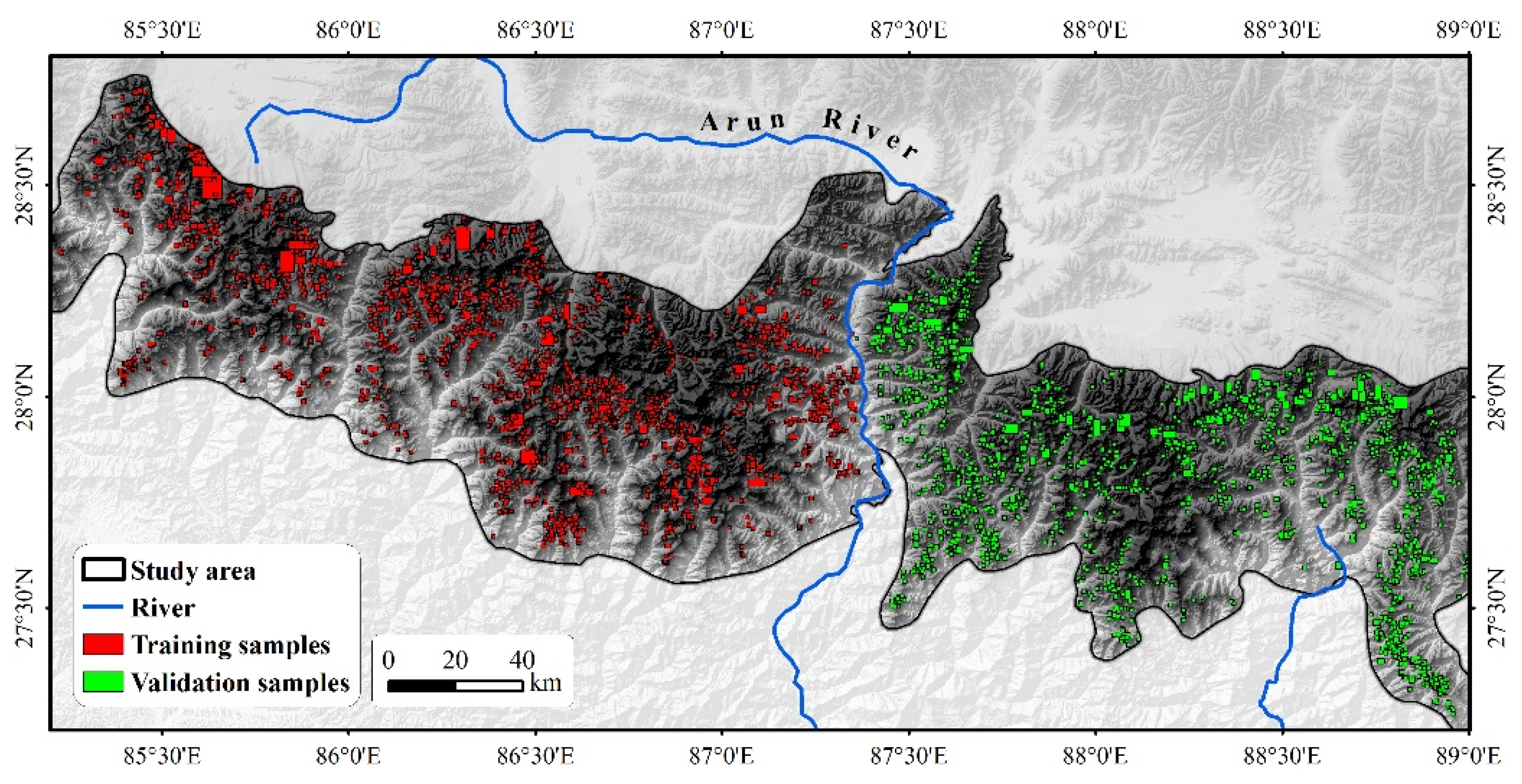
The Eastern Himalayas (85.2–89° E) is an east-west mountain range with an average elevation of 4774 m (Figure 1). A total of 2892 continental glaciers are distributed in the region, covering a total area of 3733 km2. The region has a tropical monsoon climate with an average annual temperature of −2.6 °C and annual precipitation of 1033 mm. Influenced by the Indian Ocean monsoon, the southern Eastern Himalayas has abundant rainfall and dense vegetation, whereas the northern part is desolate and dominated by an arid climate. The area is mostly covered by clouds throughout the year with only about 10% of clear days [32]. Most of the precipitation (>40%) is concentrated in the summer [33], which is the period of high geological disaster risks. Alpine lakes in the Himalayas have been growing rapidly amid climate change and glacier melting in recent decades [34], making the Eastern Himalayas one of the densest and most frequent areas of glacial lake outburst floods [35], with the highest death toll worldwide [36].
3. Data and Methods
3.1. Data
The Sentinel series of satellites are developed by the European Space Agency (ESA). The Sentinel-1 series is a C-band radar imaging mission dedicated to land and ocean monitoring, with a maximum spatial resolution of roughly 5 m. The Sentinel-2 series is a multispectral high-resolution imaging mission for land monitoring with a maximum spatial resolution of 10 m.
The ALOS PALSAR radiometrically terrain corrected (RTC) Digital Elevation Model (DEM) dataset was developed by the Alaska Satellite Facility (ASF) to provide information about elevations at 12.5-m and 30-m resolutions in GeoTIFF raster data format. We used the 12.5-m resolution dataset to meet the spatial resolution of the Sentinel images. The dataset was downloaded from the ASF Distributed Active Records Center (https://asf.alaska.edu (accessed on 4 January 2023)).
3.2. Methods
3.2.1. Data Preprocessing
The Google Earth Engine (https://earthengine.google.com (accessed on 4 January 2023)) was used for removing cloud cover and synthesizing the Sentinel-1 and Sentinel-2 summer images covering the study area between 2016 and 2020. Multiple bands, i.e., Sentinel-1 (VV (10 m)) and Sentinel-2 (Red (10 m), Green (10 m), Blue (10 m), and shortwave infrared—SWIR (20 m)), were selected to characterize the alpine lakes and their environments. The Sentinel-2 SWIR band was resampled from 20 m to 10 m to match the spatial resolution of the other bands.
Four variables were derived from the bands to enhance the representation of water, terrain, and the environment (Table 1) for training and driving deep learning networks.
As one of the most effective water indexes, the MNDWI was calculated as:
The ALOS PALSAR DEM dataset was also resampled to 10 m, and the Relief variable was derived from the DEM by calculating the difference between the maximum and minimum values within a 100 m × 100 m grid:
3.2.2. Visual Interpretation of Alpine Lakes
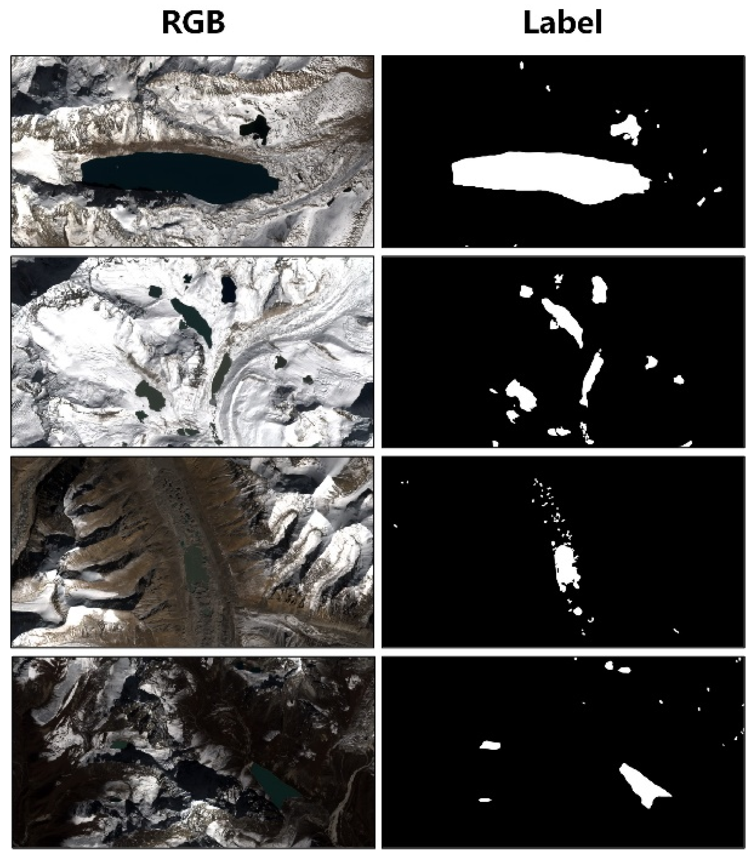
The purpose of visual analysis is to obtain data for training and validating the alpine lake identification and classification models. Three interpreters participated in the interpretation and labeled all of the lakes in the study area by visually examining the high-resolution satellite images from Google Earth; Sentinel-2 RGB images (Figure 2) were also used as a secondary reference when the RGB images were unavailable or contaminated by clouds or other factors.
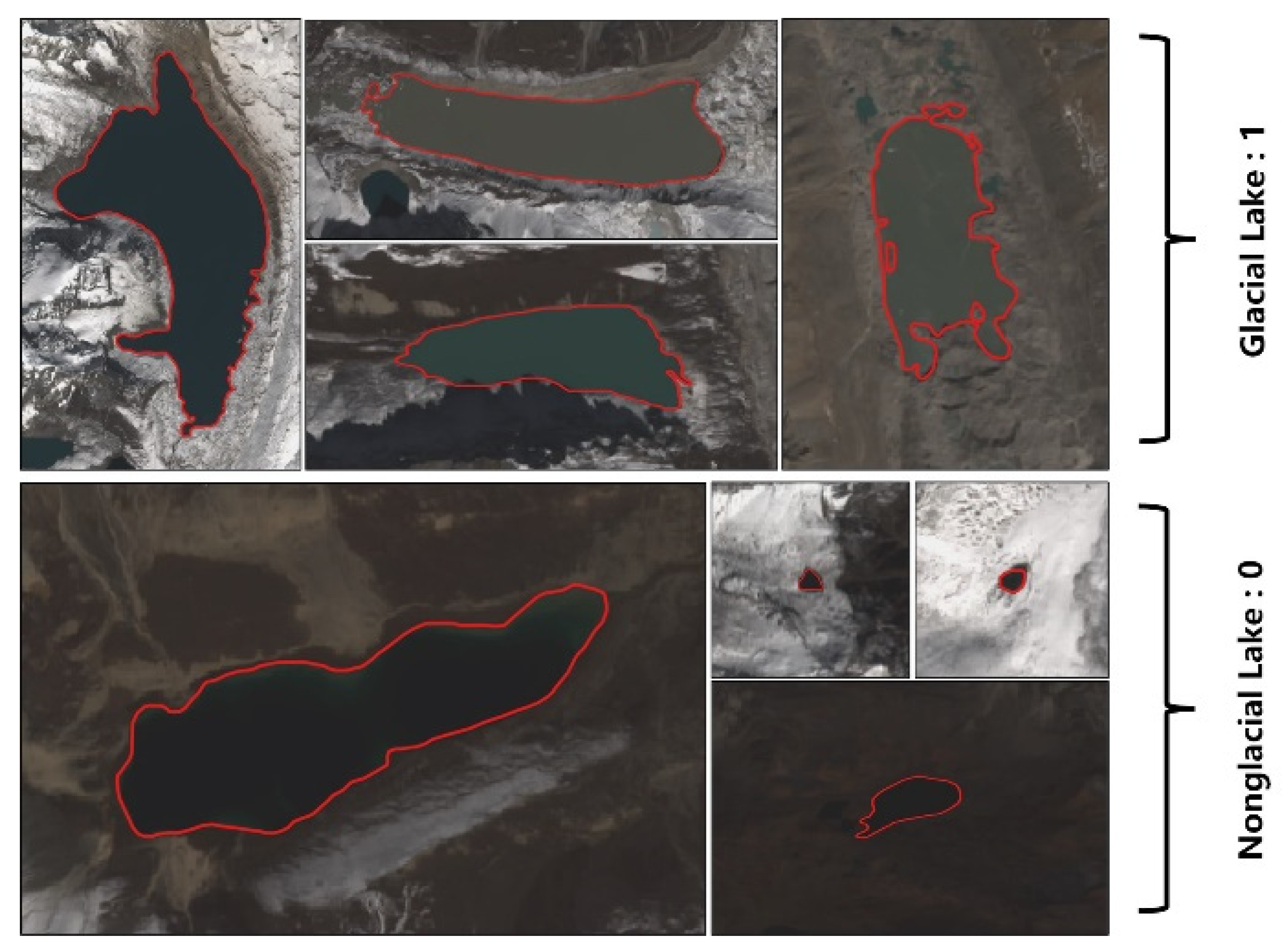
The formation of glacial or nonglacial lakes was visually determined according to their surrounding environment, such as the distance and position to the nearest glaciers and traces of glacial movement. Glacial lakes were labeled 1 and nonglacial lakes were labeled 0 (Figure 3). The outlines of the identified lakes were drawn and stored in a vector dataset with their formation types as attributes of the lake polygon features.
3.2.3. Deep Learning-Based Alpine Lake Identification
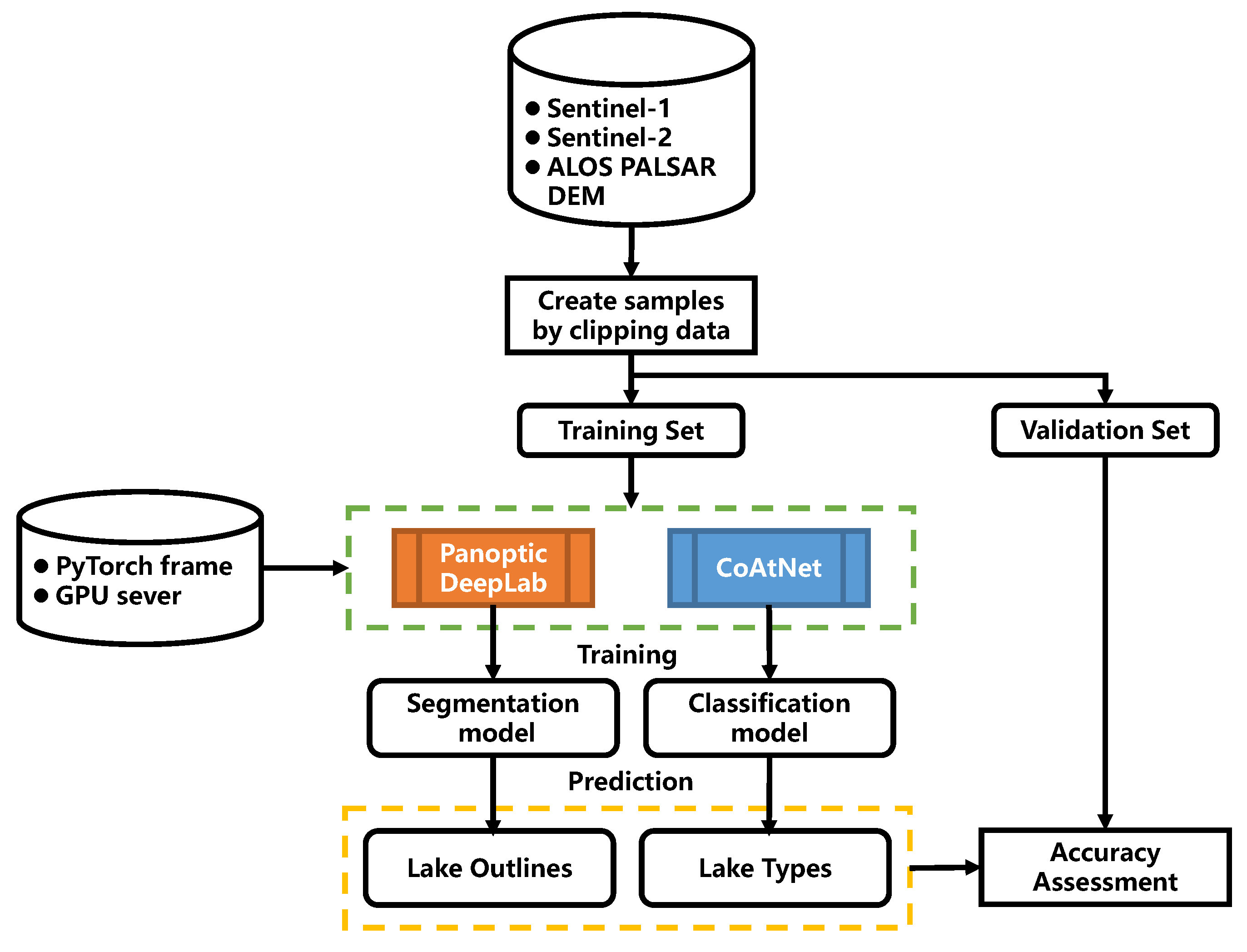
The development of a deep learning identification model for alpine lakes is given in Figure 4. The method realized the identification of the outline and type of the alpine lake through the training of two different deep learning networks.
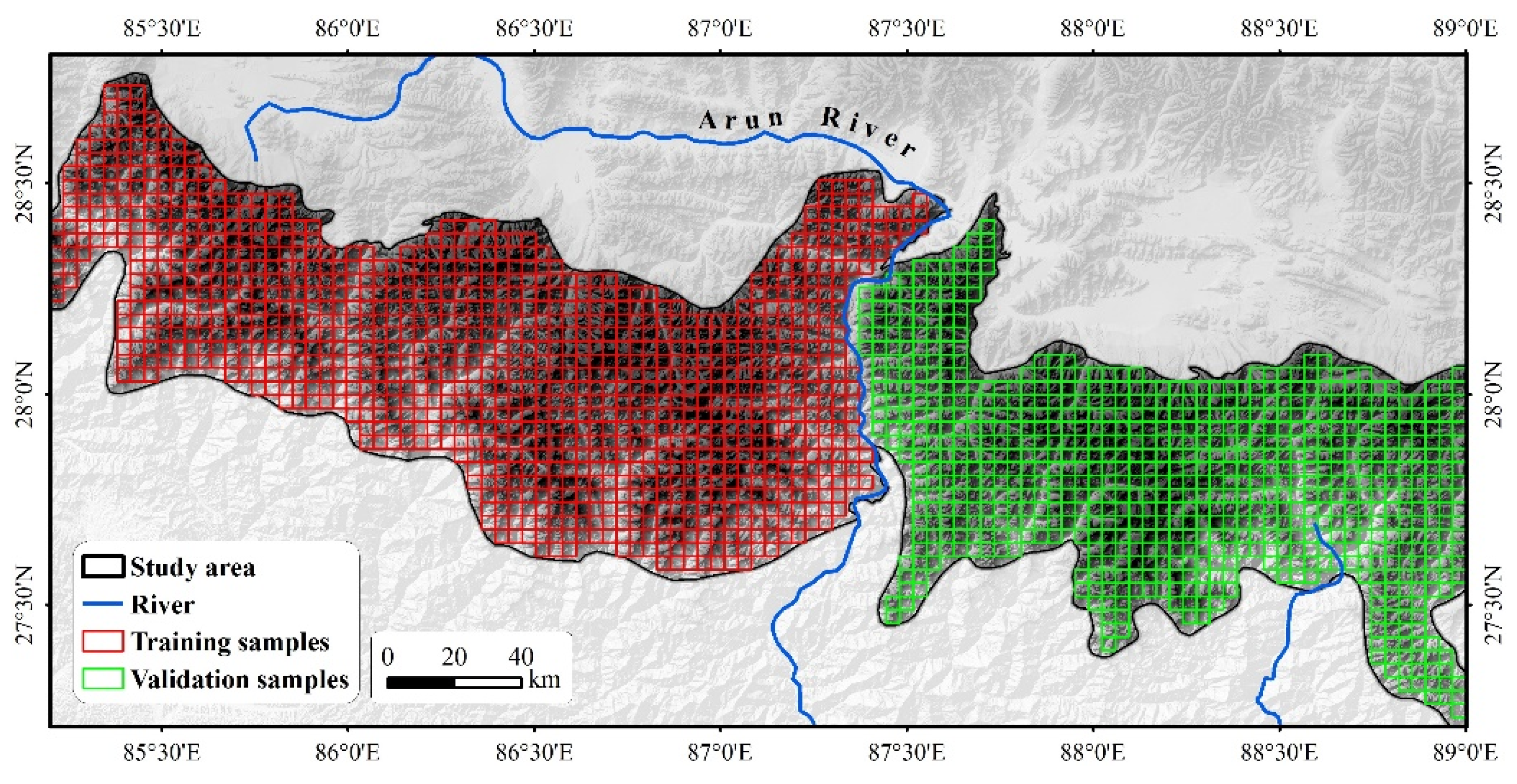
To meet the requirements of the deep learning segmentation algorithms, the study area was also divided into a systematic grid of tiles of 512 × 512 pixels with the projection of WGS 84/Pseudo-Mercator (EPSG: 3857) and a scale of 1: 5000 (Figure 5). The tiles in the study area (89,045) were divided into two groups along the Arun River. The western group of tiles (51,720) was used for training the deep learning network, and the eastern group (37,325) was reserved for validation (Table 2).
The visually labeled results were assigned to the grids to generate samples for training and validation. The tiles that intersected with the identified lakes were labeled as positive samples; otherwise, they were labeled as negative samples.
The sampling data for classification were collected by extracting the extent of each identified lake with a 300-m buffer to reflect the surrounding environment (Figure 6). A total of 4584 samples were collected (Table 3).
The identification of glacial lakes using deep learning in this paper consisted of two steps: segmentation and classification. The segmentation step detected the outlines of the glacial lakes by using a deep learning network trained from a Panoptic-DeepLab system [37]. The classification step distinguished the formation of the glacial and nonglacial lakes identified from the segmentation step using a model built from CoAtNet [38], which is a network that combines the strengths of Convolutional Neural Networks and Transformer Neural Networks.
The alpine lake segmentation model was trained from the Panoptic DeepLab network with the setup of the following parameters: (1) Backbone: HRNet-48; (2) Loss Function: Binary Dice Loss; (3) Batch size: 64; (4) positive and negative sample weights: 12.5:1. As the number of negative samples in the training data is much larger than the number of positive samples (12.5:1), the model would learn more about the features from negative samples, causing a data imbalance problem. Binary Dice Loss and sample weights were adopted to reduce the effects of data imbalance. The Binary Dice Loss training is more inclined to mining positive sample features to prevent them from being submerged by a large number of negative sample features. Increasing the weight of positive samples can increase the probability of positive samples being selected, so that the positive and negative samples could be equally effective in the training. The mean Intersection Over Union (MIoU) was calculated to measure the accuracy of the segmentation models:
where TP, FP, and FN are the true positives, false positives, and false negatives in the predictions of the trained network, respectively.
Four combinations of Sentinel-1, Sentinel-2, and DEM-derived variables (Table 4) were selected as model inputs to evaluate the alpine lake identification ability of different datasets.
The alpine lake classification model was trained from CoAtNet with the following parameters: (1) Model: CoAtNet-0; (2) Loss Function: BCE Loss; and (3) Batch size: 32. We selected four accuracy evaluation metrics to comprehensively validate the classification accuracy of the model: Overall Accuracy, User’s Accuracy, Producer’s Accuracy, and F1 Score:
3.3. Computing Environment
We set up the program running environment under a Linux system to complete the experiment. PyTorch was adopted for implementing the deep learning network framework, and the deep learning networks were trained on a computer server with 2 CPUs (Intel Xeon Gold 5118 12 Cores (Intel Corporation, Santa Clara, CA, USA)) and 16 GPUs (NVIDIA Tesla K80 12G (Nvidia Corporation, Santa Clara, CA, USA)).
4. Results
4.1. Identified Alpine Lakes
A total of 4584 alpine lakes were identified, with an average area of 0.038 km2 and an average elevation of 4974 m, including 2795 glacial lakes and 1789 nonglacial lakes (Table 5). The number, area, and elevation of the glacial lakes were greater than those of the nonglacial lakes. Most of the identified alpine lakes were small: 87% of the lakes were smaller than 0.05 km2 and 42% were smaller than 0.005 km2. A total of 32 lakes were found to be larger than 1 km2, with an average area of 1.9 km2 and the largest lake of 5.5 km2. Most glacial lakes (about 57%) were located between 5000 and 5500 m above sea level.
4.2. Segmentation Accuracy
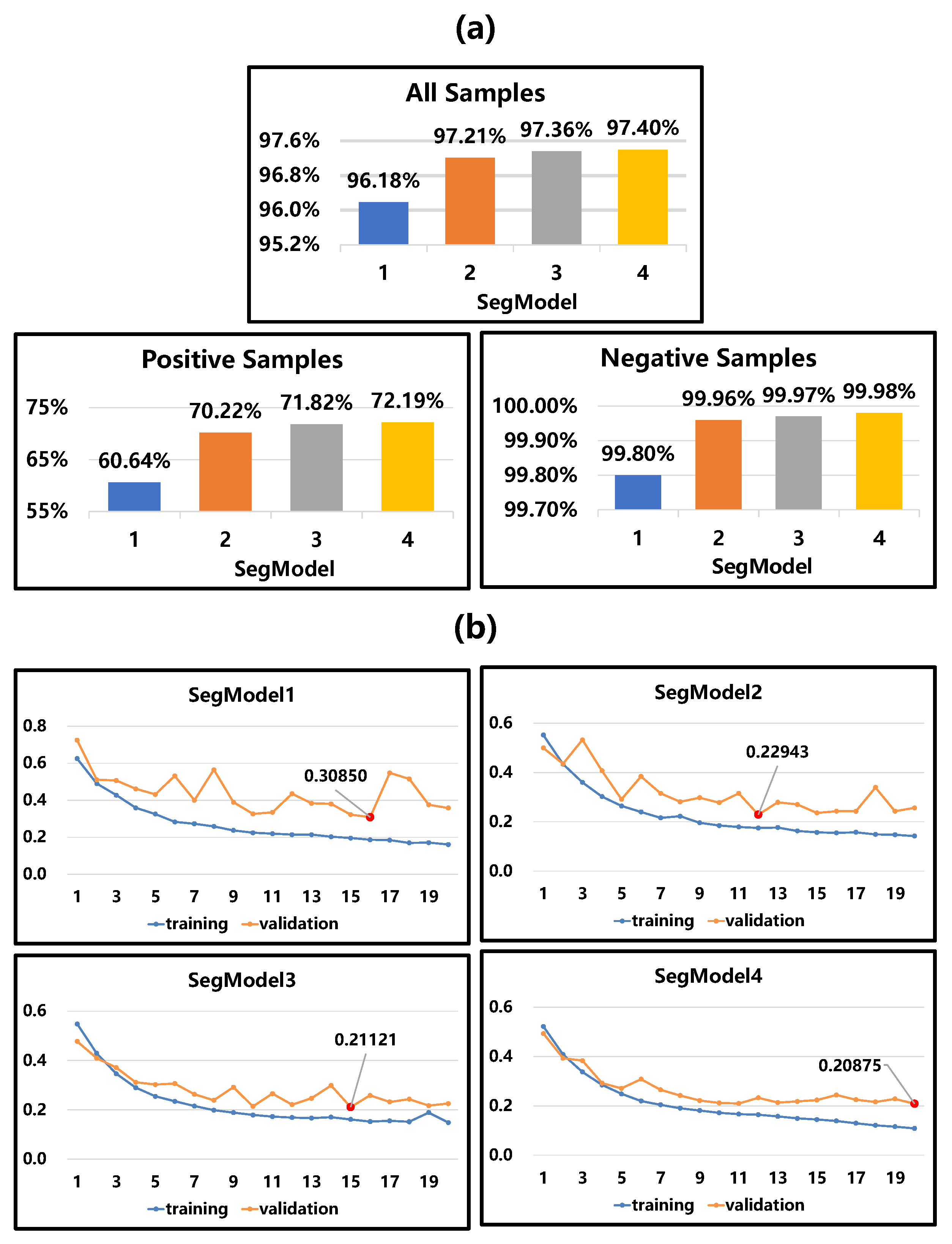
The loss of the segmentation models converged after training 20 iterations. The training loss curves were smooth, suggesting that the model achieved the imitative effect (Figure 7b). The MIoU of all samples in the four segmentation models were 96.18%, 97.21%, 97.36%, and 97.40%, respectively (Figure 7a), indicating an improved overall segmentation effect of alpine lakes as the input variables increased. The MIoU of the positive samples and the negative samples increased with the increase in input data, indicating improved completeness of alpine lakes and reduced false detection of alpine lakes as the input variables increased. In terms of the number of predicted polygons, the four segmentation models detected 1688, 1845, 1863, and 1888 lakes, respectively, of 2075 glacial lakes in the validation set. There were 3946, 1099, 928, and 841 false positive polygons in the four results, respectively. The increase in input data effectively improved the detection rate and reduced false positives.
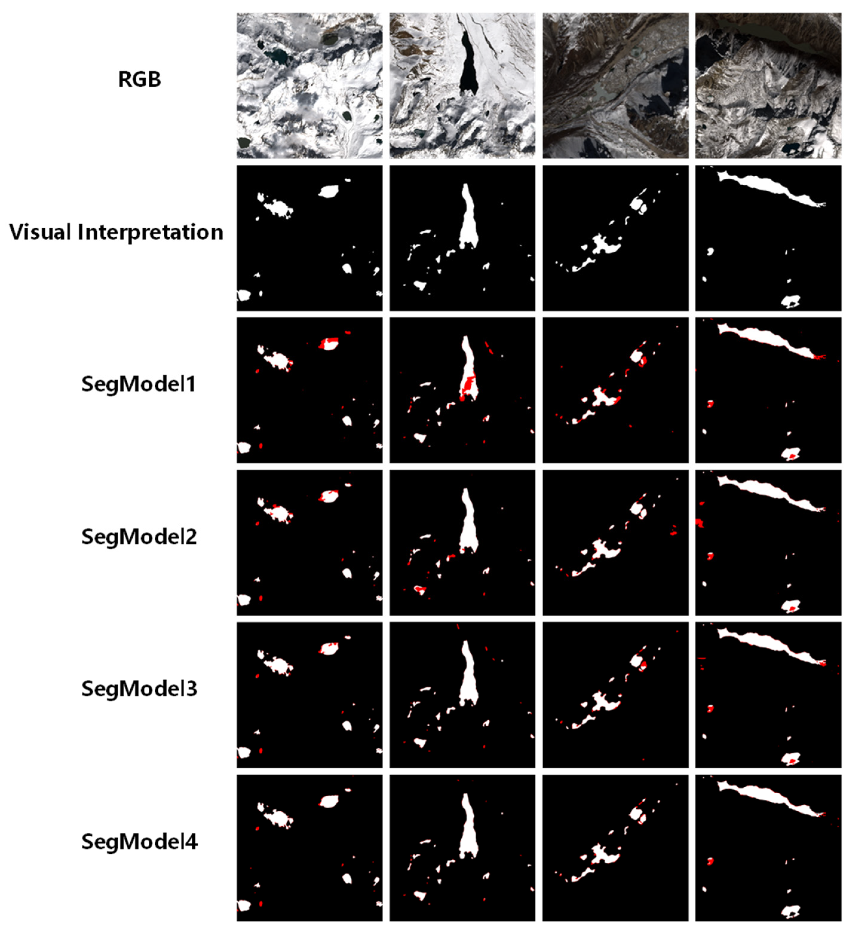
Figure 8 presents four samples from the validation data, their visual interpretation, and corresponding predictions of the four segmentation models. The SegModel1 performed worst on alpine lake completeness and error controlling. After combining the MNDWI and Sentinel-1 data, the alpine lakes predicted by the SegModel2 and SegModel3 were more complete but included more noise caused by shadows. The use of relief data significantly reduced false detection through the results of the SegModel4. Among the four segmentation models, the model that combined the four datasets was the most accurate.
4.3. Classification Accuracy
The loss of the classification model converged after 25 iterations, and each iteration took about four minutes. The best performance of the model appeared at the 18th iteration, with Overall Accuracy of 86.41%, User’s Accuracy of 86.62%, Producer’s Accuracy of 85.49%, and F1-Score of 86.05%.
Out of the 949 glacial lakes, 840 were correctly classified and yielded a Producer’s Accuracy of 88.5%, which was higher than that for nonglacial lakes (84.6%) (Table 6). However, 953 of the 1126 nonglacial lakes were correctly classified and yielded a User’s Accuracy of 89.7%, which was higher than 82.9% for glacial lakes.
5. Discussion
The combination of high-resolution satellite data and deep learning can accurately capture the distribution and characteristics of alpine lakes, particularly in the case of glacier lakes [31]. The presented method evaluated the effectiveness of identifying alpine lakes with multi-source data and the performance of distinguishing types of alpine lakes (glacial and nonglacial lakes). It suggested that multi-source satellite data, especially SAR and optical data, can greatly improve the detection rate and reduce false positives in alpine lake identification. The validation loss curves fluctuated downwards, but the variation decreased as more input variables were added, suggesting that the increase in information reduced the uncertainty of the segmentation (Figure 7b).
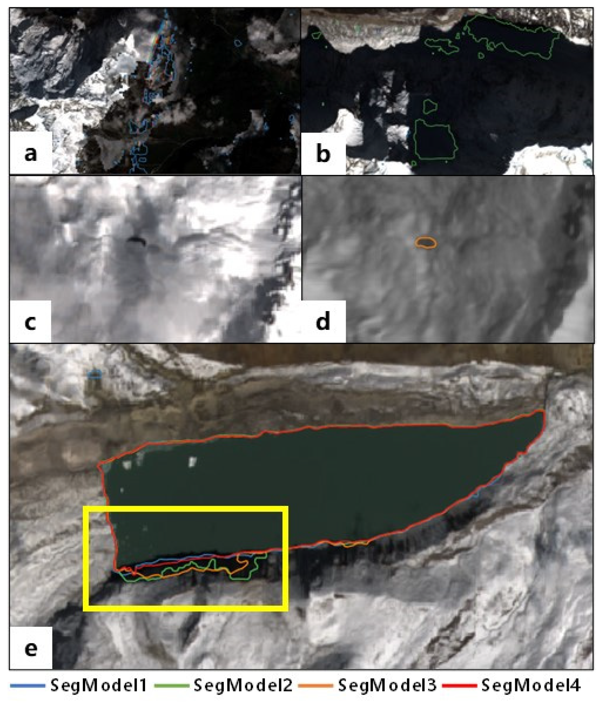
The segmentation accuracy was greatly affected by quality issues due to clouds, shadows, and other anomalies when only RGB was used as the input. These issues usually led to false positives (Figure 9a). Our experiment suggested that MNDWI could considerably improve water detection, but it is also prone to shadow effects (Figure 9b). Optical satellite data cannot penetrate clouds, leading to underestimating the number of lakes (Figure 9c); however, SAR data (VV) can overcome this limitation of optical data (Figure 9d). Additionally, SAR data are not sensitive to shallow waters. Relief data can help correcting the false positives caused by terrain shadows (Figure 9e).
The Sentinel satellite data were effective in identifying alpine lakes; however, the 10-m resolution data struggled with small moraine thaw lakes, which are hard to identify even through visual interpretation. Errors and inconsistencies in visual interpretation could be propagated into the model and affect the performance of segmentation and classification. Satellite data with higher resolutions could improve the ability to identify alpine lakes, particularly small ones. High-resolution images could also help improve the quality of interpretation by producing high-quality training data, which are key to the success of mapping alpine lakes in extreme mountainous environments.
Both deep learning models with a single RGB input (DL-RGB) and multiple inputs (DL-Multisource) produced significantly higher accuracy than the traditional approach of applying a threshold to the satellite-derived water index (MNDWI), suggesting that a deep learning method performs better for water detection (Table 7).
The MNDWI method captured most lakes in the test region, demonstrating its effectiveness in detecting water. However, the method produced many false positives, including a large number of rivers. This situation was caused by the limitation of spectral algorithm, which is not sensitive to the spatial characteristics of water bodies. The deep learning algorithm can integrate the spectral and spatial characteristics of water bodies to achieve a better identification effect. The DL-RGB method produced fewer false positives than the MNDWI, but was conservative at lake detection by capturing the least number of lakes among the three methods. The DL-Multisource method detected slightly fewer lakes than the MNDWI, with considerably fewer false positives than the other two methods, indicating that deep learning with multi-source inputs performed the best among the three methods regarding both water detection ability and misidentification.
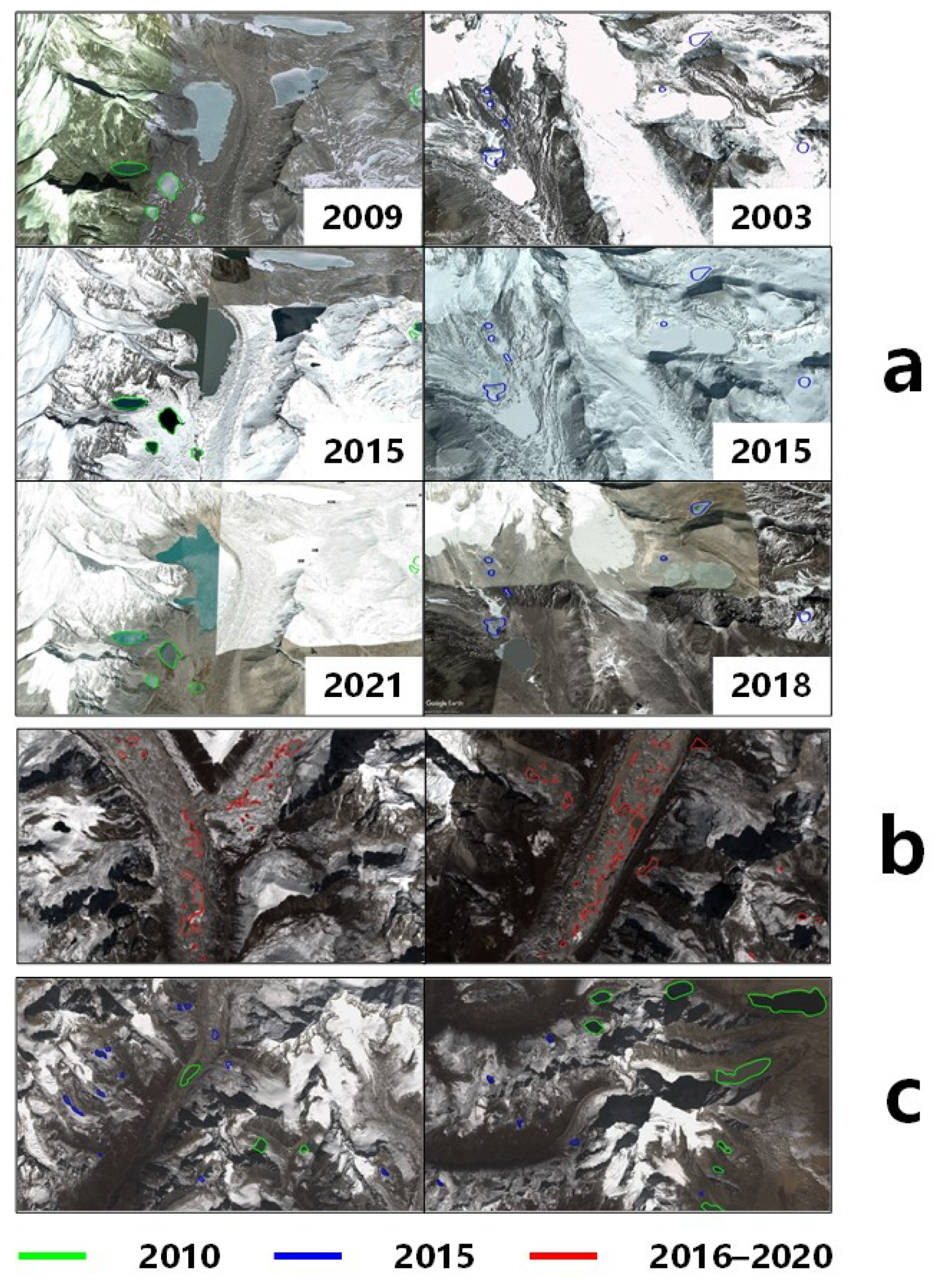
In this paper, we compiled an inventory of alpine lakes during 2016–2020 for the Eastern Himalayas, identifying 4584 lakes, including 2795 glacial lakes. We extracted the published datasets for the region and compared them to the glacial lakes in the Third Pole Environment (TPE) (V1.0) (2010) [39] and inventory data of glacial lake in western China (2015) [40]. The two datasets reported 501 and 533 lakes, less than 20% of the lakes identified by our inventory (Table 8). Although the two datasets were produced for different years (2010 and 2015), the slow temporal dynamics of alpine lakes were unlikely to cause significant differences between the datasets. The two datasets were both produced from visual interpretation of the 30-m resolution Landsat images. Examples showed glacial lakes that clearly existed between 2009 and 2018 but were missed in both datasets (Figure 10a). The coarser resolution of Landsat data could have contributed to the omission of small lakes, especially glacial thaw lakes (Figure 10b), and the lower number of reported lakes compared to our inventory, which was produced from Sentinel data.
Our inventory captured nearly all glacial lakes identified by the two reference datasets, suggesting low commission errors with our inventory compared to the two datasets. However, only 120 glacial lakes were reported by both datasets (Figure 10c). The lack of consistency between them is likely due to differences in methods and guidelines adopted by the two datasets. The comparison also signals the urgency for mapping glacial lakes at finer scales with higher-resolution satellite data to fill the gaps in our understanding of glacial lakes, especially regarding those small in size but high in numbers.
6. Conclusions
In this paper, we presented an automatic method for the identification of glacial lakes based on deep learning and multi-source satellite data, including optical and SAR data. Compared to traditional spectral-based water detection methods, the deep learning-based methods presented considerably improved water detection ability, with significantly reduced overestimation. The inclusion of a water index (MNDWI), a SAR band (Sentinel-1 VV), and a terrain band (Relief), in addition to RGB images, as inputs for the deep learning method further improved the model performances. Although the transferability of the model has been evaluated in eastern Himalayas, the model may not perform well in regions outside of the Himalayas due to limited representation in the training data. Incorporating the training data of other regions would further improve the model’s ability for identifying alpine lakes worldwide.
An alpine lake inventory consisting of 2075 glacial and 1789 nonglacial lakes was compiled for the Eastern Himalayas; this value is five times higher than the previously reported number of glacial lakes in the two previously existing datasets. The inventory unveiled a large number of glacial lakes that were missed by the existing datasets, especially small glacial thaw lakes, indicating considerable knowledge gaps. The combination of deep learning and multi-source high-solution satellite data demonstrated great potential for mapping small alpine lakes in extreme environments in the Himalayas and other part of the world, such as in Greenland and Antarctica. The results will provide critical information for understanding these ecosystems and early warning of glacial lake outburst floods.
Author Contributions
M.F., J.X. and Y.S. designed the research concept. Y.S., K.Z. and K.S. performed the data collection for experiments. J.X. implemented the automated alpine lake identification method and analyzed the results. M.F. and J.X. drafted the manuscript. D.Y. contributed to the data visualization. All authors discussed and reviewed the paper prior to submission. All authors have read and agreed to the published version of the manuscript.
Funding
This research was funded by the National Natural Science Foundation of China (42171140).
Data Availability Statement
Alpine lake inventory data set to this article can be found online at https://doi.org/10.11888/Cryos.tpdc.300056 (accessed on 4 January 2023).
Conflicts of Interest
The authors declare no conflict of interest.
References
- Füreder, L.; Ettinger, R.; Boggero, A.; Thaler, B.; Thies, H. Macroinvertebrate Diversity in Alpine Lakes: Effects of Altitude and Catchment Properties. Hydrobiologia 2006, 562, 123–144. [Google Scholar] [CrossRef]
- Fitzsimons, S.; Howarth, J. Chapter 9—Glaciolacustrine Processes. In Past Glacial Environments, 2nd ed.; Menzies, J., van der Meer, J.J.M., Eds.; Elsevier: Amsterdam, The Netherlands, 2018; pp. 309–334. ISBN 978-0-08-100524-8. [Google Scholar]
- Chen, X.; Cui, P.; Li, Y.; Yang, Z.; Qi, Y. Changes in Glacial Lakes and Glaciers of Post-1986 in the Poiqu River Basin, Nyalam, Xizang (Tibet). Geomorphology 2007, 88, 298–311. [Google Scholar] [CrossRef]
- Fujita, K.; Sakai, A.; Nuimura, T.; Yamaguchi, S.; Sharma, R.R. Recent Changes in Imja Glacial Lake and Its Damming Moraine in the Nepal Himalaya Revealed by Surveys and Multi-Temporal ASTER Imagery. Environ. Res. Lett. 2009, 4, 045205. [Google Scholar] [CrossRef]
- Wang, X.; Liu, S.; Ding, Y.; Guo, W.; Jiang, Z.; Lin, J.; Han, Y. An Approach for Estimating the Breach Probabilities of Moraine-Dammed Lakes in the Chinese Himalayas Using Remote-Sensing Data. Nat. Hazards Earth Syst. Sci. 2012, 12, 3109–3122. [Google Scholar] [CrossRef] [Green Version]
- Haeberli, W. Glacier and Permafrost Signals of 20th-Century Warming. Ann. Glaciol. 1990, 14, 99–101. [Google Scholar] [CrossRef] [Green Version]
- Quincey, D.J.; Richardson, S.D.; Luckman, A.; Lucas, R.M.; Reynolds, J.M.; Hambrey, M.J.; Glasser, N.F. Early Recognition of Glacial Lake Hazards in the Himalaya Using Remote Sensing Datasets. Glob. Planet. Chang. 2007, 56, 137–152. [Google Scholar] [CrossRef]
- Bajracharya, B.; Shrestha, A.B.; Rajbhandari, L. Glacial Lake Outburst Floods in the Sagarmatha Region. Mred 2007, 27, 336–344. [Google Scholar] [CrossRef] [Green Version]
- Schwanghart, W.; Worni, R.; Huggel, C.; Stoffel, M.; Korup, O. Uncertainty in the Himalayan Energy–Water Nexus: Estimating Regional Exposure to Glacial Lake Outburst Floods. Environ. Res. Lett. 2016, 11, 074005. [Google Scholar] [CrossRef] [Green Version]
- Das, S.; Kar, N.S.; Bandyopadhyay, S. Glacial Lake Outburst Flood at Kedarnath, Indian Himalaya: A Study Using Digital Elevation Models and Satellite Images. Nat. Hazards 2015, 77, 769–786. [Google Scholar] [CrossRef]
- Winsvold, S.H.; Kääb, A.; Nuth, C. Regional Glacier Mapping Using Optical Satellite Data Time Series. IEEE J. Sel. Top. Appl. Earth Obs. Remote Sens. 2016, 9, 3698–3711. [Google Scholar] [CrossRef]
- McFeeters, S.K. The Use of the Normalized Difference Water Index (NDWI) in the Delineation of Open Water Features. Int. J. Remote Sens. 1996, 17, 1425–1432. [Google Scholar] [CrossRef]
- Xu, H. A Study on Information Extraction of Water Body with the Modified Normalized Difference Water Index (MNDWI). J. Remote Sens.-BeiJing 2005, 9, 595. [Google Scholar]
- Feyisa, G.L.; Meilby, H.; Fensholt, R.; Proud, S.R. Automated Water Extraction Index: A New Technique for Surface Water Mapping Using Landsat Imagery. Remote Sens. Environ. 2014, 140, 23–35. [Google Scholar] [CrossRef]
- Bolch, T.; Buchroithner, M.F.; Peters, J.; Baessler, M.; Bajracharya, S. Identification of Glacier Motion and Potentially Dangerous Glacial Lakes in the Mt. Everest Region/Nepal Using Spaceborne Imagery. Nat. Hazards Earth Syst. Sci. 2008, 8, 1329–1340. [Google Scholar] [CrossRef] [Green Version]
- Bolch, T.; Peters, J.; Yegorov, A.; Pradhan, B.; Buchroithner, M.; Blagoveshchensky, V. Identification of Potentially Dangerous Glacial Lakes in the Northern Tian Shan. In Terrigenous Mass Movements: Detection, Modelling, Early Warning and Mitigation Using Geoinformation Technology; Pradhan, B., Buchroithner, M., Eds.; Springer: Berlin/Heidelberg, Germany, 2012; pp. 369–398. ISBN 978-3-642-25495-6. [Google Scholar]
- Li, J.; Sheng, Y. An Automated Scheme for Glacial Lake Dynamics Mapping Using Landsat Imagery and Digital Elevation Models: A Case Study in the Himalayas. Int. J. Remote Sens. 2012, 33, 5194–5213. [Google Scholar] [CrossRef]
- Wangchuk, S.; Bolch, T.; Zawadzki, J. Towards Automated Mapping and Monitoring of Potentially Dangerous Glacial Lakes in Bhutan Himalaya Using Sentinel-1 Synthetic Aperture Radar Data. Int. J. Remote Sens. 2019, 40, 4642–4667. [Google Scholar] [CrossRef]
- Zhang, B.; Liu, G.; Zhang, R.; Fu, Y.; Liu, Q.; Cai, J.; Wang, X.; Li, Z. Monitoring Dynamic Evolution of the Glacial Lakes by Using Time Series of Sentinel-1A SAR Images. Remote Sens. 2021, 13, 1313. [Google Scholar] [CrossRef]
- Ferretti, A.; Massonnet, D.; Monti-Guarnieri, A.; Prati, C.; Rocca, F. Guidelines for SAR Interferometry Processing and Interpretation. In InSAR Principles; Fletcher, K., Ed.; ESA Publications Division: Noordwijk, The Netherlands, 2007; Available online: http://www.esa.int/About_Us/ESA_Publications/InSAR_Principles_Guidelines_for_SAR_Interferometry_Processing_and_Interpretation_br_ESA_TM-19 (accessed on 4 January 2023).
- Yao, X.; Liu, S.; Han, L.; Sun, M.; Zhao, L. Definition and Classification System of Glacial Lake for Inventory and Hazards Study. J. Geogr. Sci. 2018, 28, 193–205. [Google Scholar] [CrossRef] [Green Version]
- Chen, F.; Zhang, M.; Tian, B.; Li, Z. Extraction of Glacial Lake Outlines in Tibet Plateau Using Landsat 8 Imagery and Google Earth Engine. IEEE J. Sel. Top. Appl. Earth Obs. Remote Sens. 2017, 10, 4002–4009. [Google Scholar] [CrossRef]
- Rounce, D.R.; Watson, C.S.; McKinney, D.C. Identification of Hazard and Risk for Glacial Lakes in the Nepal Himalaya Using Satellite Imagery from 2000–2015. Remote Sens. 2017, 9, 654. [Google Scholar] [CrossRef] [Green Version]
- Raj, K.B.G.; Kumar, K.V. Inventory of Glacial Lakes and Its Evolution in Uttarakhand Himalaya Using Time Series Satellite Data. J. Indian Soc. Remote Sens 2016, 44, 959–976. [Google Scholar] [CrossRef]
- Wangchuk, S.; Bolch, T. Mapping of Glacial Lakes Using Sentinel-1 and Sentinel-2 Data and a Random Forest Classifier: Strengths and Challenges. Sci. Remote Sens. 2020, 2, 100008. [Google Scholar] [CrossRef]
- Qayyum, N.; Ghuffar, S.; Ahmad, H.M.; Yousaf, A.; Shahid, I. Glacial Lakes Mapping Using Multi Satellite PlanetScope Imagery and Deep Learning. ISPRS Int. J. Geo-Inf. 2020, 9, 560. [Google Scholar] [CrossRef]
- Wu, R.; Liu, G.; Zhang, R.; Wang, X.; Li, Y.; Zhang, B.; Cai, J.; Xiang, W. A Deep Learning Method for Mapping Glacial Lakes from the Combined Use of Synthetic-Aperture Radar and Optical Satellite Images. Remote Sens. 2020, 12, 4020. [Google Scholar] [CrossRef]
- Thati, J.; Ari, S. A Systematic Extraction of Glacial Lakes for Satellite Imagery Using Deep Learning Based Technique. Measurement 2022, 192, 110858. [Google Scholar] [CrossRef]
- Wang, J.; Chen, F.; Zhang, M.; Yu, B. NAU-Net: A New Deep Learning Framework in Glacial Lake Detection. IEEE Geosci. Remote Sens. Lett. 2022, 19, 1–5. [Google Scholar] [CrossRef]
- Wang, J.; Chen, F.; Zhang, M.; Yu, B. ACFNet: A Feature Fusion Network for Glacial Lake Extraction Based on Optical and Synthetic Aperture Radar Images. Remote Sens. 2021, 13, 5091. [Google Scholar] [CrossRef]
- Wang, S.; Peppa, M.V.; Xiao, W.; Maharjan, S.B.; Joshi, S.P.; Mills, J.P. A Second-Order Attention Network for Glacial Lake Segmentation from Remotely Sensed Imagery. ISPRS J. Photogramm. Remote Sens. 2022, 189, 289–301. [Google Scholar] [CrossRef]
- Drusch, M.; Del Bello, U.; Carlier, S.; Colin, O.; Fernandez, V.; Gascon, F.; Hoersch, B.; Isola, C.; Laberinti, P.; Martimort, P.; et al. Sentinel-2: ESA’s Optical High-Resolution Mission for GMES Operational Services. Remote Sens. Environ. 2012, 120, 25–36. [Google Scholar] [CrossRef]
- Daac, O. MODIS and VIIRS Land Products Global Subsetting and Visualization Tool; ORNL DAAC: Oak Ridge, TN, USA, 2017. [Google Scholar] [CrossRef]
- Maurer, J.M.; Schaefer, J.M.; Rupper, S.; Corley, A. Acceleration of Ice Loss across the Himalayas over the Past 40 Years. Sci. Adv. 2019, 5, eaav7266. [Google Scholar] [CrossRef]
- Carrivick, J.L.; Tweed, F.S. A Global Assessment of the Societal Impacts of Glacier Outburst Floods. Glob. Planet. Chang. 2016, 144, 1–16. [Google Scholar] [CrossRef]
- Veh, G.; Korup, O.; Walz, A. Hazard from Himalayan Glacier Lake Outburst Floods. Proc. Natl. Acad. Sci. USA 2020, 117, 907–912. [Google Scholar] [CrossRef] [PubMed]
- Cheng, B.; Collins, M.D.; Zhu, Y.; Liu, T.; Huang, T.S.; Adam, H.; Chen, L.-C. Panoptic-Deeplab: A Simple, Strong, and Fast Baseline for Bottom-up Panoptic Segmentation. In Proceedings of the IEEE/CVF Conference on Computer Vision and Pattern Recognition, Seattle, WA, USA, 13–19 June 2020; pp. 12475–12485. [Google Scholar]
- Dai, Z.; Liu, H.; Le, Q.V.; Tan, M. CoAtNet: Marrying Convolution and Attention for All Data Sizes. arXiv 2021, arXiv:2106.04803. [Google Scholar]
- Zhang, G. Data on Glacial Lakes in the TPE (V1.0) (1990, 2000, 2010); National Tibetan Plateau Data Center: Beijing, China, 2018. [Google Scholar]
- Wang, X. Inventory Data of Glacial Lake in West China (2015); National Tibetan Plateau Data Center: Beijing, China, 2018. [Google Scholar]
Figure 1.
Study area in the Eastern Himalayas (85.2–89° E).

Figure 2.
Examples of Sentinel-2 RGB composites of alpine lakes and corresponding labels used for segmentation.
Figure 2.
Examples of Sentinel-2 RGB composites of alpine lakes and corresponding labels used for segmentation.

Figure 3.
Examples of alpine lakes and corresponding labels used for classification.

Figure 4.
Flow diagram of the methods in the study.

Figure 5.
Distribution of training and validation sample tiles in the segmentation dataset.

Figure 6.
Distribution of training and validation samples used for classification.

Figure 7.
Comparison of four segmentation models in the training and validation process: (a) MIoU; (b) loss.
Figure 7.
Comparison of four segmentation models in the training and validation process: (a) MIoU; (b) loss.

Figure 8.
Example results predicted by the four segmentation models (red indicates where predicted results do not match visual interpretation).
Figure 8.
Example results predicted by the four segmentation models (red indicates where predicted results do not match visual interpretation).

Figure 9.
Advantages and problems in different scenarios: (a) False positives caused by using only true color images. (b) False positives extracted by MNDWI due to shadows. (c) A lake covered in clouds (d) was extracted after the addition of VV. (e) Shadow removal after adding Relief data.
Figure 9.
Advantages and problems in different scenarios: (a) False positives caused by using only true color images. (b) False positives extracted by MNDWI due to shadows. (c) A lake covered in clouds (d) was extracted after the addition of VV. (e) Shadow removal after adding Relief data.

Figure 10.
Comparison of lake inventories from different years: (a) We found some glacial lakes that were not mapped in the 2010 and 2015 inventories, according to historical images from different periods obtained from Google Earth. (b) Most glacial thaw lakes were not mapped in the 2010 and 2015 inventories. (c) Lack of consistency between the 2010 and 2015 inventories.


Table 1.
Input variables derived for training and driving deep learning networks, including the Sentinel-1 vertical-vertical (VV) dual polarization SAR data, Sentinel-2 red-green-blue (RGB) and MNDWI variables, and the Relief variable derived from the ALSO PALSAR DEM.
Table 1.
Input variables derived for training and driving deep learning networks, including the Sentinel-1 vertical-vertical (VV) dual polarization SAR data, Sentinel-2 red-green-blue (RGB) and MNDWI variables, and the Relief variable derived from the ALSO PALSAR DEM.
| Data Source | Variables | Data Type |
|---|---|---|
| Sentinel-1 | VV | SAR |
| Sentinel-2 | RGB, MNDWI | Optical |
| ALOS PALSAR | Relief | DEM |
Table 2.
Number of total, positive, and negative tiles in the study area used for training and validation.
Table 2.
Number of total, positive, and negative tiles in the study area used for training and validation.
| Training | Validation | Total | |
|---|---|---|---|
| Positive | 3938 | 3476 | 7414 |
| Negative | 47,782 | 33,849 | 81,631 |
| Total | 51,720 | 37,325 | 89,045 |
Table 3.
Number of glacial and nonglacial lakes in the study area used for training and validation.
| Training | Validation | Total | |
|---|---|---|---|
| Glacial Lakes | 1881 | 949 | 2795 |
| Nonglacial Lakes | 663 | 1126 | 1789 |
| Total | 2544 | 2075 | 4584 |
Table 4.
Input data combinations for driving the segmentation models.
| Training Scenarios | Inputs |
|---|---|
| SegModel1 | RGB |
| SegModel2 | RGB, MNDWI |
| SegModel3 | RGB, MNDWI, VV |
| SegModel4 | RGB, MNDWI, VV, Relief |
Table 5.
Area, number, and elevation of the identified alpine lakes (glacial and nonglacial); Differences derived from median of all the identified and interpreted alpine lakes.
Table 5.
Area, number, and elevation of the identified alpine lakes (glacial and nonglacial); Differences derived from median of all the identified and interpreted alpine lakes.
| Number | Area (km2) | Elevation (m) | ||||||||
|---|---|---|---|---|---|---|---|---|---|---|
| Sum | Min | Max | Mean | Difference | Min | Max | Mean | Difference | ||
| Glacial Lakes | 2795 | 148 | 4 × 10⁻⁴ | 5.5 | 5.3 × 10⁻² | 1.7 × 10⁻⁴ | 3690 | 5971 | 5145 | 11 |
| Nonglacial Lakes | 1789 | 42 | 4 × 10⁻⁴ | 2.1 | 2.4 × 10⁻² | −6.6 × 10⁻⁴ | 1496 | 5890 | 4706 | 27 |
Table 6.
Confusion matrix of the alpine lake classification.
| Visual Interpretation | |||||
|---|---|---|---|---|---|
| Glacial Lakes | Nonglacial Lakes | Total | User’s Accuracy | ||
| Prediction | Glacial Lakes | 840 | 173 | 1013 | 82.9% |
| Nonglacial Lakes | 109 | 953 | 1062 | 89.7% | |
| Total | 949 | 1126 | |||
| Producer’s Accuracy | 88.5% | 84.6% | |||
Table 7.
Comparison of three methods for identifying alpine lakes.
| MNDWI | DL-RGB | DL-Multisource | |
|---|---|---|---|
| Visual Interpretation Number | 2075 | 2075 | 2075 |
| Detected Lakes Number | 1939 | 1688 | 1888 |
| False Positives Number | 8161 | 3946 | 841 |
| MIoU | 88.55% | 96.18% | 97.40% |
Disclaimer/Publisher’s Note: The statements, opinions and data contained in all publications are solely those of the individual author(s) and contributor(s) and not of MDPI and/or the editor(s). MDPI and/or the editor(s) disclaim responsibility for any injury to people or property resulting from any ideas, methods, instructions or products referred to in the content. |
© 2023 by the authors. Licensee MDPI, Basel, Switzerland. This article is an open access article distributed under the terms and conditions of the Creative Commons Attribution (CC BY) license (https://creativecommons.org/licenses/by/4.0/).
Share and Cite
MDPI and ACS Style
Xu, J.; Feng, M.; Sui, Y.; Yan, D.; Zhang, K.; Shi, K. Identifying Alpine Lakes in the Eastern Himalayas Using Deep Learning. Water 2023, 15, 229. https://doi.org/10.3390/w15020229
AMA Style
Xu J, Feng M, Sui Y, Yan D, Zhang K, Shi K. Identifying Alpine Lakes in the Eastern Himalayas Using Deep Learning. Water. 2023; 15(2):229. https://doi.org/10.3390/w15020229
Chicago/Turabian StyleXu, Jinhao, Min Feng, Yijie Sui, Dezhao Yan, Kuo Zhang, and Kaidan Shi. 2023. "Identifying Alpine Lakes in the Eastern Himalayas Using Deep Learning" Water 15, no. 2: 229. https://doi.org/10.3390/w15020229
Note that from the first issue of 2016, this journal uses article numbers instead of page numbers. See further details here.