Assessing Groundwater Evolution with a Combined Approach of Hydrogeochemical Modelling and Data Analysis: Application to the Rhodope Coastal Aquifer (NE Greece)

Abstract

Assessing the hydrogeochemical evolution of groundwater is a challenging task, which is further exacerbated when considering the multiple geogenic and anthropogenic impacts that affect its quality and the hydraulic interactions between different aquifer bodies. This study combined hydrogeochemical modelling and data analysis to assess this complex hydrogeological regime. Before modelling, the groundwater samples were clustered using a multivariate statistical method (hierarchical cluster analysis (HCA)). Then, the Geochemist Workbench (GWB) software was applied to model the hydrogeochemical groundwater evolution, including the dominant ion exchange process, and to explain the changes in groundwater chemistry towards its flow. The input data consisted of five key parameters from seventy-seven sampling points collected in two periods (accounting for the start and the end of the irrigation period). A data analytical approach based on the optimal mixing ratios between the interacting groundwater systems and recharge inputs was also performed as part of the methodological approach. It revealed a progressively temporal-dependent behaviour of the aquifer system during the irrigation period, resulting in seasonal changes in the hydrodynamic conditions and depletion of the upper aquifer layers. Specifically, the aquifer system was confirmed to undergo cation exchange as the dominant geochemical process that increases calcium concentrations. The complex hydrogeological regime was further evaluated by assessing the mixing ratios of the different aquifer layers. Hence, the aquifer system (bulk samples) was mixed with the irrigation water by 71% and 97% and with the lateral recharge by 76% and 29% for the beginning and at the end of the irrigation period, respectively. Overall, the joint assessments were confirmed by the hydrogeochemical status of the end-members and the modelling approach and explained the sequential changes in groundwater chemistry due to the dominant ion-exchange process and the mixing of different water bodies. The proposed methodological approach proved that it could be used as an exploratory and preliminary method for capturing the temporal dynamics in complex groundwater systems and supporting groundwater resource management.

1. Introduction

Groundwater constitutes a vital freshwater resource of significant importance for multiple uses. Comprehending its evolution in time and space, including both qualitative and quantitative characteristics, is a critical step towards sustainable groundwater resource management and decision-making. Groundwater science has used several tools and methods to assess or quantify its evolution. A widespread approach for hydrogeochemical evaluations combines common hydrochemical analysis to identify the principal processes and water types using various plots (e.g., Piper and ionic ratio plots) and diagrams (e.g., Gibbs and Wilcox), along with spatial interpolation maps and multivariate statistical analysis (Q-mode and R-mode) (e.g., [1,2,3]). However, this well-rounded approach lacks the identification of the water–rock interaction through modelling [2] and provides a limited outlook for sustainable management [3]. In [4], the suitability of groundwater consumption and irrigation water quality was assessed by using classic hydrochemical analysis, PHREEQC code, and various other water quality indices. In [5,6], an alternative approach of multivariate statistical analysis was used by utilizing the results of the chemical analysis and the measured indices with a partial least squares regression model (PLSR) for a more accurate assessment of groundwater quality.

Groundwater modelling offers insights to decision-makers for sustainable management of groundwater resources; however, limitations or lack of data can affect the results of the models’ calibration. The application of a 3D transient density-dependent groundwater model can be used for a comprehensive evaluation of seawater intrusion [7], quantification of the impact of the overexploitation of groundwater reserves [8], and assessment of the natural and artificial groundwater recharge [9].

The inverse or forwarding hydrogeochemical modelling is often used to identify the mixing processes in an aquifer system and the evolution of groundwater. In [10], a mixing inverse model is performed between virtual and real samples using the VISHMOD method, while in [11,12], an inverse model is combined with palaeogeological, hydrogeochemical, and multivariate statistical techniques. A reactive transport model using the MIN3D code is combined with stable isotope fractionation to simulate the hydrogeochemical processes in [13].

Multivariate statistical analysis (MVSA) is widely used to interpret the evolution characteristics of groundwater resources, usually paired with hydrogeochemical methods (e.g., ion plots, hydrochemical facies evolution diagram (HFE-D), Gibbs diagram, Wilcox diagram, and boxplots) [14], and with water quality indices [15]. Integrated multivariate statistical methods for groundwater quality evaluation, as in [16], in which principal component analysis (PCA) is coupled with correlation analysis, hydrogeochemical analysis, and multiple linear regression model, provide a more comprehensive approach. In [17], hydrogeochemical analysis is coupled with hierarchical cluster analysis (HCA) and paired with the Bregman block average algorithm (BBAC_I) to identify the spatial and temporal patterns of groundwater geochemistry separately (HCA) and simultaneously (BBAC_I). A double clustering approach using HCA on an entire dataset and then on defined groups of variables paired with hydrogeochemical analysis to delineate the major processes and spatial distribution of the major and minor elements in groundwater is applied [18].

The use of environmental isotopes coupled with the approaches mentioned above is quite frequent for the efficient monitoring and management of groundwater quality. In [19], isotopic analysis is coupled with a hydrochemical, multivariate statistical approach and with a groundwater quality index, which is preferable to be used if there is limited information on land use and hydrogeology to assess groundwater quality. In [20], stable isotopes, hydrochemical data, and hydrogeochemical modelling using PHREEQC are combined to define the hydrochemical evolution, characterization, and protection of groundwater. Integrating different approaches (e.g., hydrochemical and inverse modelling) coupled with isotopic analysis is also applied in [21,22].

A mixing cell model (MCM) is used to define and decipher groundwater’s intricate origin, mixing, and water–rock interaction [23]. The multivariate mixing and mass balance model (M3) mainly use water–rock interaction and compares the major ionic components, stable isotopes, and tritium to determine the chemical evolutions of groundwater. Certain errors in hydrochemical data, faulty conceptualization, and methodological errors constitute the model’s uncertainties. In [24], a groundwater model is paired with an inverse MCM, which is validated by incorporating a forward MCM using the mean cell residence time derived from ¹⁴C.

Classic hydrogeological approaches combine all or some of the tools mentioned above (e.g., [25,26]), while new approaches, as in [27], introduce the use of artificial intelligence-based models to predict the complex seawater intrusion evolution in coastal aquifers.

These methods incorporate inherent advantages and drawbacks, which include specific site characteristics, data quality and availability, and expert knowledge. Hence, selecting an optimal method to be applied heavily depends on the above requisites and often includes a combination of different approaches. However, that could be time-consuming and complex when there is a need for a preliminary evaluation, which in turn could provide insight into the main optimal method(s) to be selected for the main assessment.

Therefore, the need for an exploratory and accurate approach emerges to facilitate the overall assessment, especially when the sites under investigation are constituted of complex hydrogeological systems with increased heterogeneity. Towards this aim, an exploratory method able to shed light on groundwater evolution, either applied as a stand-alone tool or as the basis for more sophisticated approaches applied at a later stage, is proposed in this study.

The present research aims to provide a preliminary conceptualization of the groundwater evolution of a complex hydrogeological system using a combined hydrogeochemical modelling and data analytical approach. As an outcome, we model the evolution of groundwater from the coastal areas to the inland and quantify the contribution of each aquifer layer and other sources (irrigation water and recharge inflows) to the final groundwater chemistry of selected parameters.

2. Geological and Hydrogeological Setting

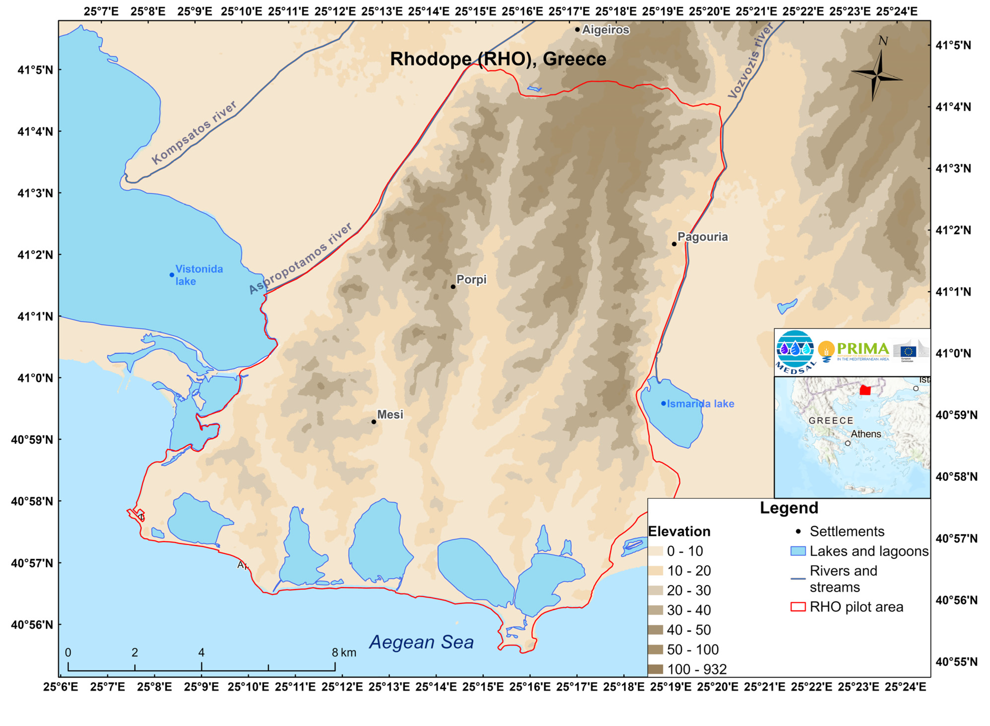
The study area to which the proposed combined hydrogeochemical approach is applied lies in north-eastern Greece (Thrace), with an approximate coverage of 110 km² (Figure 1). It extends between Vistonida and Ismarida Lakes from west to east, and the northern boundary is oriented by a hydrogeological barrier of a clay aquitard across the east to west direction northern of Pagouria village. The southern orientation follows the coastline. The climate of the study area is characterized as warm-summer Mediterranean climate (Csb) according to the updated Köppen climate classification [28]. Available raw climate data for the study area is provided by two stations: the SWAT_RHO station and the IMEROS-MARONIA station. The SWAT_RHO station is a grid point located in the study area that belongs to the Global Weather Database for SWAT. The IMEROS-MARONIA station is a meteorological station that belongs to the meteorological stations’ network of the National Observatory of Athens, which is continuously operational since 2 July 2010 till present and provides daily temperature, precipitation, and wind speed data. According to the available data, the mean annual precipitation and reference evapotranspiration for the period 1979–2014 at the local SWAT_RHO station were estimated to be 603 and 1256 mm, respectively, while the values for the Imeros-Maronia station were estimated to be 498 and 1098 mm, respectively.

The hydrogeological system consists of two main aquifers. According to [29], the upper one is a semi-confined aquifer of poor quality due to the elevated salinity. It was developed during recent alluvial deposits (sand, gravel, etc.) with a high clay content. The lower confined aquifer developed during the Miocene–Pliocene formations (marls, sandstones, etc.) generally has significantly better quality with low salinity. The two aquifers are not in direct hydraulic contact, as a clay aquitard of a few centimetres to meters practically disrupts any crossflow [29].

Both aquifers are used for irrigation, as the Rhodope coastal area is mainly characterized by agricultural land use. However, the contribution of each aquifer is unknown, as nearly all boreholes are exploiting both, with no specific information about the depth of filters in the casing. Thus, the exploited groundwater is a mix of both aquifer layers with unknown proportions.

Groundwater quality in the study area is heavily affected by salinization, predominantly triggered by seawater intrusion from the SW and SE parts of the coastline, according to [30]. Piezometry ranges from a few meters to approximately 45–50 m below mean sea level in the deepest parts of the system [29]. Groundwater flows to the central part towards a depression area driven by tectonics. The main recharge of the system is from its western parts through the lateral crossflows of the Kompsatos River alluvial fan [29].

3. Material and Methods

Data from 57 boreholes were sampled in two campaigns (P1 and P2) conducted in June and August 2020. The sampling network was selected with the basic criterion of being representative of the spatial coverage of the area, as well as additional conditions (e.g., accessibility of wells and operational use). The sampling periods were selected intentionally to coincide with the start (P1) and the end (P2) of the irrigation period and to capture the system’s temporal variations. The sampling followed the standard procedure (e.g., boreholes were operating for irrigation during sampling or were set to operate for at least 30 min prior to sampling). The aliquot intended for the major ion analyses was filtered with a 0.45μ cellulose membrane and stored in cool conditions. The specific conductance (SPC) and the other physicochemical parameters (e.g., pH, DO, and ORP) were measured in situ with portable instruments (YSI In-situ 9000). The samples were analyzed using various parameters, including major ions (photometrically and by atomic absorption spectroscopy (AAS)) and trace elements (AAS with furnace graphite), following the standard methods for the examination of water [31].

The quality control (QC) and quality assurance (QA) of the analytical results were confirmed by the calculation of the charge balance error (CBE = {[Σcations − Σanions]/[Σcations + Σanions]} × 100) and duplicate/replicate analyses (4 pairs). Two samples exhibited CBE above 10% and were eliminated from further data processing. The rest exhibited CBE < 10%, which was considered acceptable for further handling [32]. The analysis of duplicates/replicates showed negligible deviations (<3%) for all critical parameters. The results of the selected parameters used in the modelling and data analytical procedure are shown in

Table 1. Selected chemical parameters for the samples used in the model of P1.

Parameters		Samples
		G1	G2	G3s4	G3s5	IR	RE	CE1	CE2
	Ca2+ (mg/L)	76.35	204.4	492.8	749.5	35.75	30.26	864.6	615.4
	Mg+ (mg/L)	20	51.65	129	216.5	6.65	12.64	367.4	282.5
	Na+ (mg/L)	98.86	113.1	157.4	629.6	111.9	21.93	653.7	192.2
	Si2+ (mg/L)	14.06	13.7	12	7.59	17.5	1	723.7	727.3
	Cl− (mg/L)	145.3	543.3	1382	2514	136.8	17.73	2626	1291

and

Table 2. Selected chemical parameters for the samples used in the model of P2.

Parameters	G1	G2	G3s5	G3s6	IR	RE	CE1	CE2
Ca2+ (mg/L)	65.6	88.6	749.5	517.5	30.85	30.26	1235	471.7
Mg+ (mg/L)	15	23.4	216.5	130.1	5.4	12.64	409.3	114.5
Na+ (mg/L)	90.98	108.2	629.6	233.6	156.15	21.93	421.8	234.2
Si2+ (mg/L)	13.53	13.82	7.59	13.87	16.6	1	726.1	2.321
Cl− (mg/L)	142.7	191.6	2514	1486	146.85	17.73	3034	1437

.

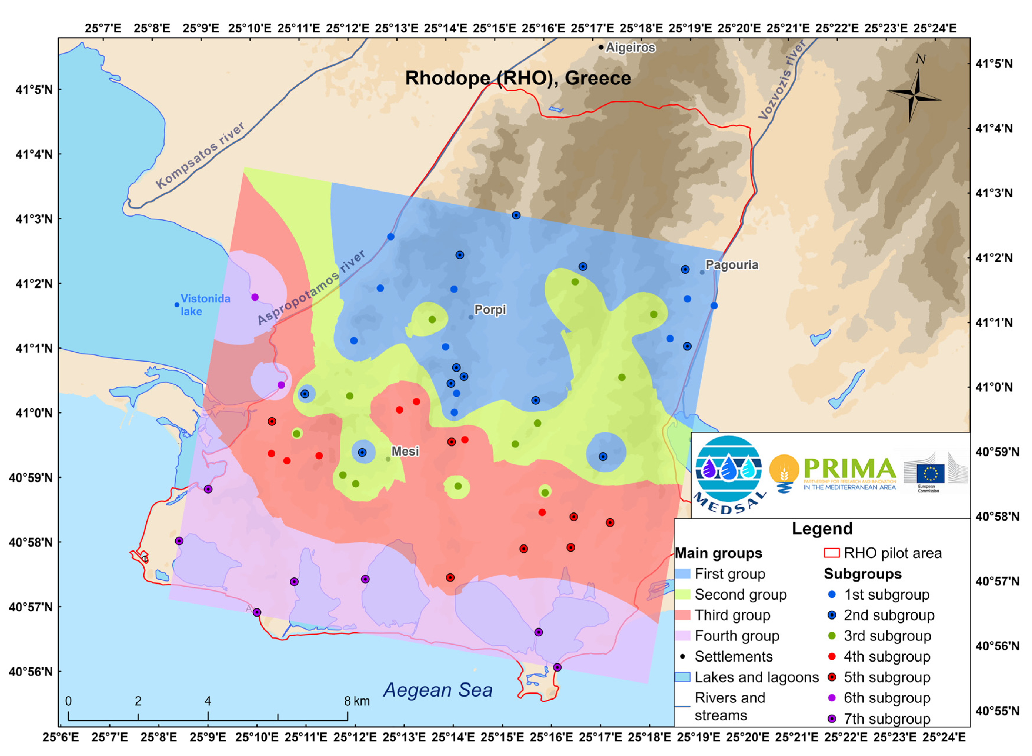
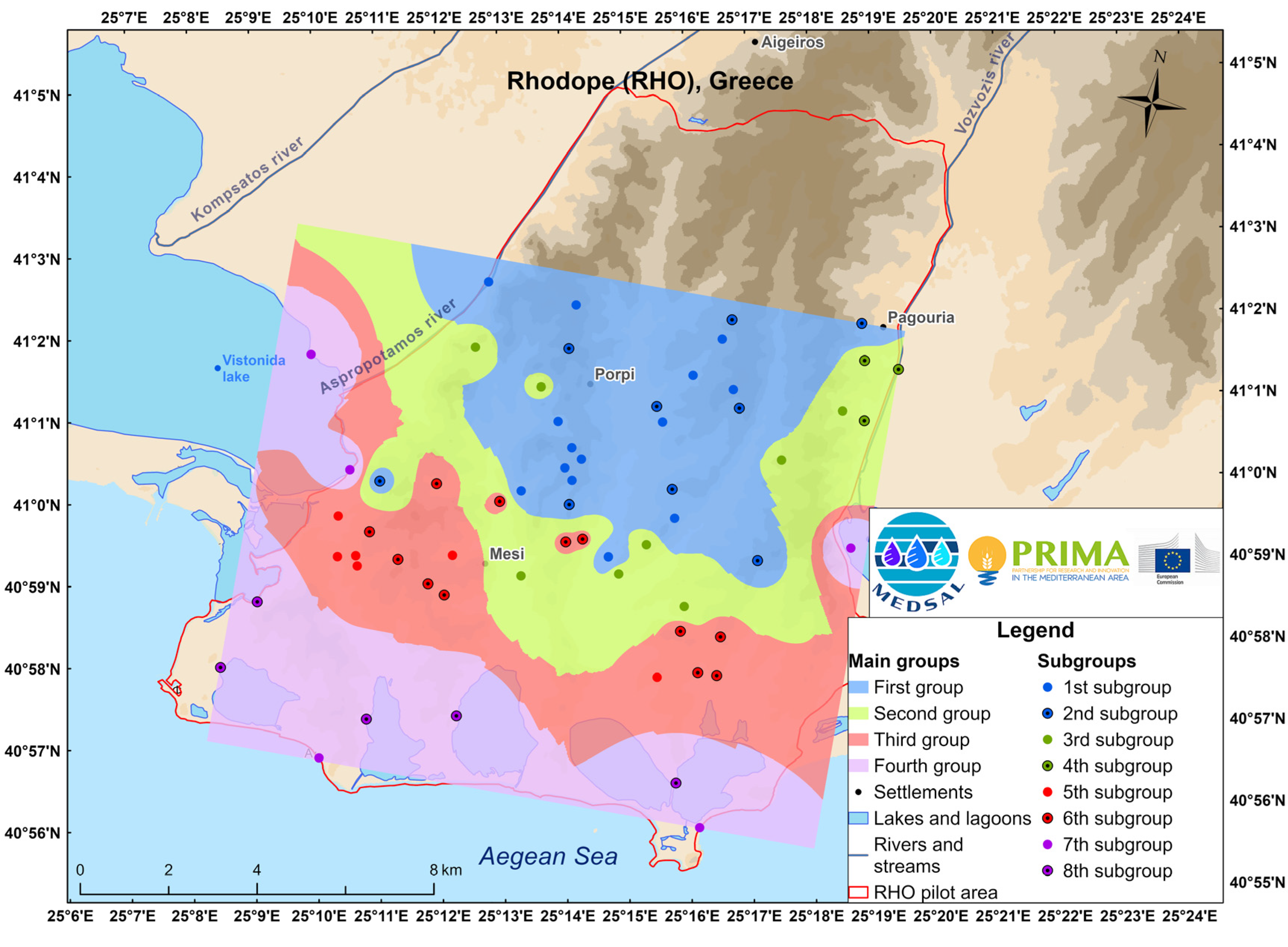
The data were further processed using hierarchical cluster analysis (HCA) after being checked for the requirements for applying multivariate statistics (e.g., normal or log-normal distribution). If the normality criterion was not met, a transformation was applied (Johnson transformation); all data were standardized via z-scores. HCA was selected to classify the samples according to their hydrogeochemical characteristics and to identify their latent similarities. The results classified the samples into four major groups and seven or eight subgroups, as shown in Figure 2 and Figure 3 for P1 and P2, respectively. The four major groups identified the dominant classes based on the hydrogeochemistry of the samples. However, a more thorough classification within the subgroups was performed by categorizing the major groups into subgroups, denoting further differences and/or patterns of their hydrogeochemistry. The derived results were interpolated with the IDW method and outlined the spatial distribution of each factor for both periods. According to Figure 2 and Figure 3, we may infer a zonation from the coastline to the inland, which spatially orients the impact on groundwater chemistry from different processes towards the groundwater flow.

The conceptualization and testing of the possible groundwater evolution scenarios (models) were performed by processing the key findings of the HCA with (a) the mode “react” of the GWB 12 software ^®(Aqueous Solutions LLC, Champaign, IL 61820, USA) to simulate and quantify the cation exchange process, and with (b) the Microsoft Excel Solver to reach an optimal mathematical output of groundwater mixing. The methodological sequence is described below.

The principal equation used for the calculation with the “solver” is as follows:

C₁V₁ + C₂V₂ = C_mixV_mix,

(1)

where C₁ and V₁ are the concentration and the volume of the first initial sample; C₂ and V₂ are the concentration and the volume of the second initial sample; and C_mix and V_mix are the concentration and the volume of the modelled (mix) sample.

V₁ + V₂ = V_mix = 1 (constant)

(2)

The optimal mix ratio of the volumes of the initial samples is selected according to the minimum sum of the subtracted absolute values of the initial samples Σ|Cmix_i − Ct_i| (Equation (2)), where “i” is the selected parameter each time (e.g., Ca and Mg). The Ct value is the measured value of the “ith” parameter (according to the analytical results) for the final (target) sample. The lowest absolute sum (difference from the target mix) defined the optimal percentage of volumes of the initial solutes. Considering this approach, the estimated mixing result of all parameters should present the lowest possible deviation of the concentrations compared to the final target sample (Ct).

According to [33], using the median compositions of each group (virtual samples) from a clustering procedure (e.g., HCA) as model inputs facilitates rapid convergence and produces more robust models by minimizing the inherent variability between individual samples. Thus, in our case, the modelling exercise used the “virtual” samples of the groups (G) and subgroups (s) obtained from the applied HCA for both periods. These “virtual” samples are composed of the median values of selected parameters for each group and subgroup, which are Ca²⁺, Mg²⁺, Na⁺, Si²⁺, and Cl⁻. These parameters were selected based on two criteria: (a) participating in the dominant process related to salinization or water–rock interaction (e.g., Ca²⁺, Mg²⁺, Na⁺, and Si²⁺) and/or (b) having a conservative character (Cl⁻) during groundwater flow. Hence, they could all be regarded as representative of the dominant cation exchange process and groundwater evolution.

The geochemical process of (reverse) ion (cation) exchange is identified as the key process for the SW part of the study area, due to the active seawater intrusion ([29,30]). Specifically, the Ca-rich clays (reported to be abundant in that area) exchange Ca for Na (included as NaCl in seawater), thus enriching the aqueous solution with calcium.

In addition to the virtual samples, two more key samples were used: (a) the IR sample, which is considered to be representative of the irrigation water and is abstracted from the confined (deeper) aquifer, and (b) the RE, which is considered to be representative of the recharge water (the dominant recharge flow) from the alluvial fan of the Kompsatos River (the dominant recharge of the systems from the NW). All the other water samples (CE1 and CE2) are the products of cation exchange or mixing of the samples described above and were modelled using the GWB software.

The combined modelling approach was performed for both periods (P1 and P2) to identify potential temporal changes of the system between the start and the end of the irrigation period, during which the hydrodynamic conditions could have possibly changed. The period at the end of the irrigation period (end of the warm-dry period) describes the conditions after abstracting all the required groundwater for covering irrigation demand with negligible inflows from rainfall or other sources. In contrast, the period before the start of the irrigation season (end of the wet-cold season) describes the conditions after groundwater recovery by the autumn-winter inflows from rainfall or other sources.

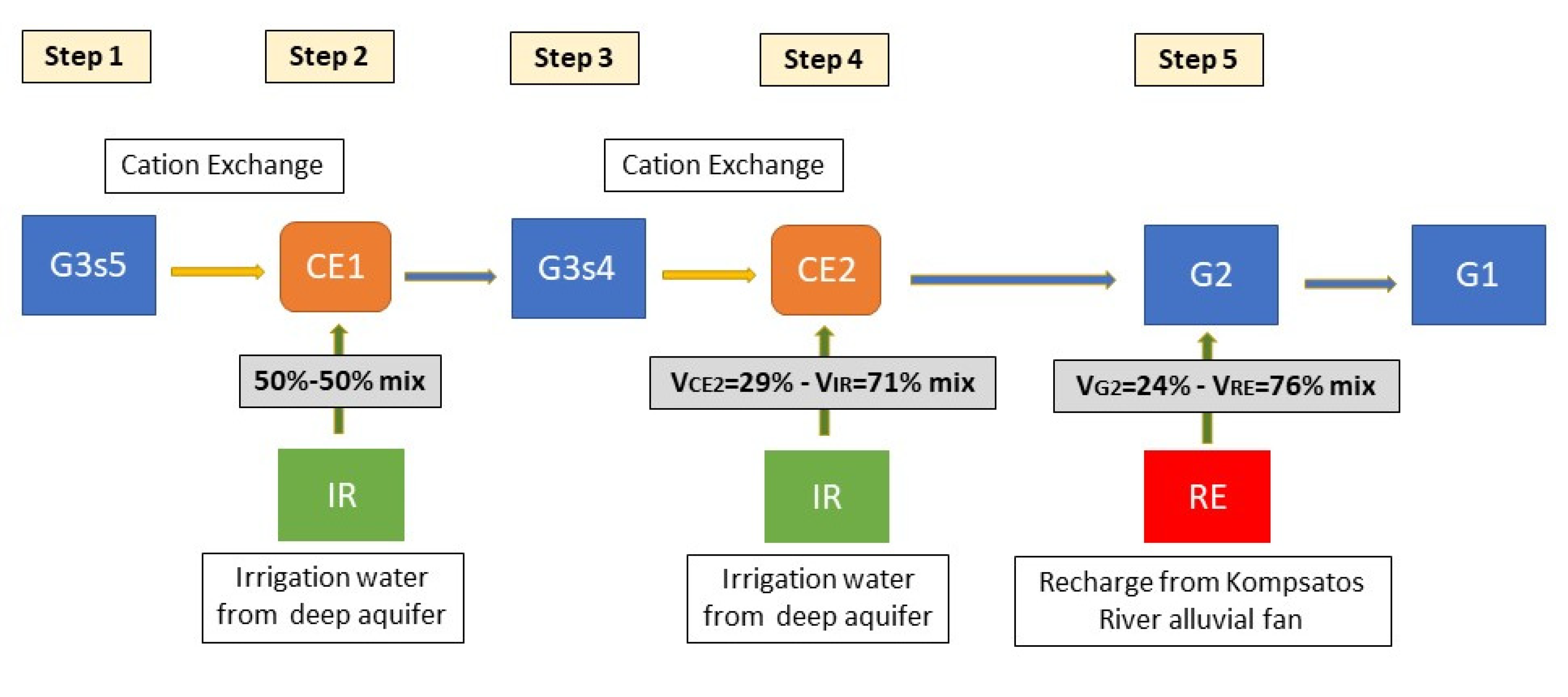
The methodological array of the modelling for both periods includes five discrete steps:

Step 1: Modelling cation exchange by using an initial solution that reacts with a predefined quantity of clay minerals (5 mmols of smectite and kaolinite, both reported as abundant in the area [30].

Step 2: Mixing the upper aquifer (product of step 1) with irrigation water (IR) from the deeper confined aquifer.

Step 3: Modelling cation exchange by using an initial solution of the product of step 2 and similar conditions of clay content as step 1.

Step 4: Mixing the upper aquifer (product of step 3) with irrigation water (IR) from the deeper confined aquifer.

Step 5: Mixing step 4 product with recharge water (RE) (lateral crossflows from the Komspatos River alluvial fan).

According to the chemical analytical results and the HCA outcomes, the above five steps were selected consecutively as a possible evolution scenario. The two possible scenarios for P1 and P2 align with the current hydrogeological knowledge of the area and the irrigation conditions (exploitation of both aquifer layers with unknown proportions).

4. Results and Discussion

4.1. Modelling of P1 (Start of Irrigation Period)

The model for P1, as explained, used the “virtual” samples (median values) of the groups and subgroups obtained from the HCA (accounting for the P1 period), namely G1, G2, G3s4 (Group 3, subgroup 4), and G3s5 (Group 3, subgroup 5). Their chemical compositions are shown in Table 1. The IR samples were selected according to their chemistry and spatial position in conjunction with the water groups/subgroups they belong to and their adjacent (surrounding) samples. Specifically, the IR samples have a significantly different chemistry than the adjacent ones. They belong to the G1 group (which occurs as outliers within the G2 and G3 zones), which is probably typical for the lower (deeper) aquifer of better quality. The RE sample is based on two (2) selected boreholes of the Hellenic Groundwater Monitoring Network [34]. The selected boreholes are sampled four times per year. The value used is the median of the two boreholes that account for the samples of the cold-wet period (November to April). As mentioned, the CE1 and CE2 samples are the products of the modelling procedure (cation exchange).

The P1 model (Figure 4) consists of five sequential steps as described below. The target is to model the cation exchange process and to mix the samples with the appropriate volumes to obtain, as an outcome, a sample as close (in terms of chemistry) to G1 as possible.

Step 1: The G3s5 sample is submitted to cation exchange (CE1), as indicated by its subgroup’s dominant water type (Ca-Cl). It was assumed that the CE concerns only Ca²⁺. The modelling is performed using the mode “react” of the GWB 12 software® (Aqueous Solutions LLC, Champaign, IL 61820, USA). The initial solution is the G3s5, and the reactants are smectite and kaolinite. Previous surveys report both minerals [30] as significant and abundant in the area. The assumed quantity used is 5 mmol for each mineral. After the model run, we obtain the sample CE1, which chemistry is shown in Table 1.

Step 2: The CE1 sample (obtained from step 1) is mixed with IR to obtain G3s4 as an outcome. That is decided, as we need freshwater input to reduce the chemical concentrations of CE1 and reach G3s4. Precipitation is also tried as a fresh alternative source, but the overall required volumes surpass the mean precipitation reported for the area, which is low for that particular period.

With the aid of the “solver” data analysis (xls), we calculate the optimal volumes of CE1 and IR to reach as close as possible the chemistry of G3s4 using the equation: C_CE1 ∗ V_CE1 + C_IR ∗ V_IR = C_mix ∗ V_{mix (=1)}

If V_mix = 1 and is solved by C_mix, we obtain the concentrations of the final mix’s individual five parameters. Then, these concentrations are subtracted from the C_G3s4 (target mix sample), and their absolute difference ABS (Cmix-CG3s4) is calculated. The optimal ratio of volumes of the initial samples (V_CE1 and V_IR) is selected from the combination, which minimizes the sum of the ABS (C_mix-C_G3s4) values.

Finally, the concentrations of the targeted mix sample C_G3s4 are better approached when the two volumes are mixed equally (V_CE1 = V_IR = 50%).

Step 3: The G3s4 sample is submitted to cation exchange (CE2), as indicated by its subgroup’s dominant water type (Ca-Cl). It is assumed that the CE concerns only Ca²⁺. The modelling is performed using the mode “react” of the GWB 12 software ^®. The initial solution is the G3s4, and the reactants are smectite and kaolinite. Previous surveys report both minerals (Petalas and Diamantis, 2006) as significant and abundant clay minerals. The assumed quantity used is 5 mmol for each mineral. After the model run, we obtain the sample CE2, which chemistry is shown in Table 2.

Step 4: The CE2 sample (obtained from step 3) is mixed with IR to obtain G2 as the outcome. That is decided, as we need freshwater input to reduce the chemical concentrations of CE2 and reach G2. Precipitation is also tried as a fresh alternative source, but the overall required volumes surpass the mean precipitation reported for the area. By applying Equation (1), we calculate the optimal volumes of CE2 and IR to reach as close as possible the chemistry of G2 as follows: C_CE2 ∗ V_CE2 + C_IR ∗ V_IR = C_mix ∗ V_{mix (=1)}

If V_mix =1 and is solved by C_mix, we obtain the concentrations of the final mix’s individual five parameters. Then, these concentrations are subtracted from the C_G2 (target mix sample) and their absolute difference ABS (C_mix-C_G2) is calculated. The optimal ratio of volumes of the initial samples (V_CE2 and V_IR) is selected from the combination, which minimizes the sum of the ABS (C_mix-C_G2) values.

Finally, the concentrations of the targeted mix sample C_G2 are better approached when the two volumes are mixed as V_CE2 = 29% and V_IR = 71%.

Step 5: As reported, G2 receives an amount of freshwater from the recharge of the Kompsatos River alluvial fan. We hypothesize that this water is also mixed with G2, following the mixing of CE2 with IR. Following a similar process as described in the previous steps, the concentrations of the targeted mix sample C_G1 are better approached when the two volumes are mixed as V_G2 = 24% and V_RE = 76%.

4.2. Modelling of P2 (End of Irrigation Period)

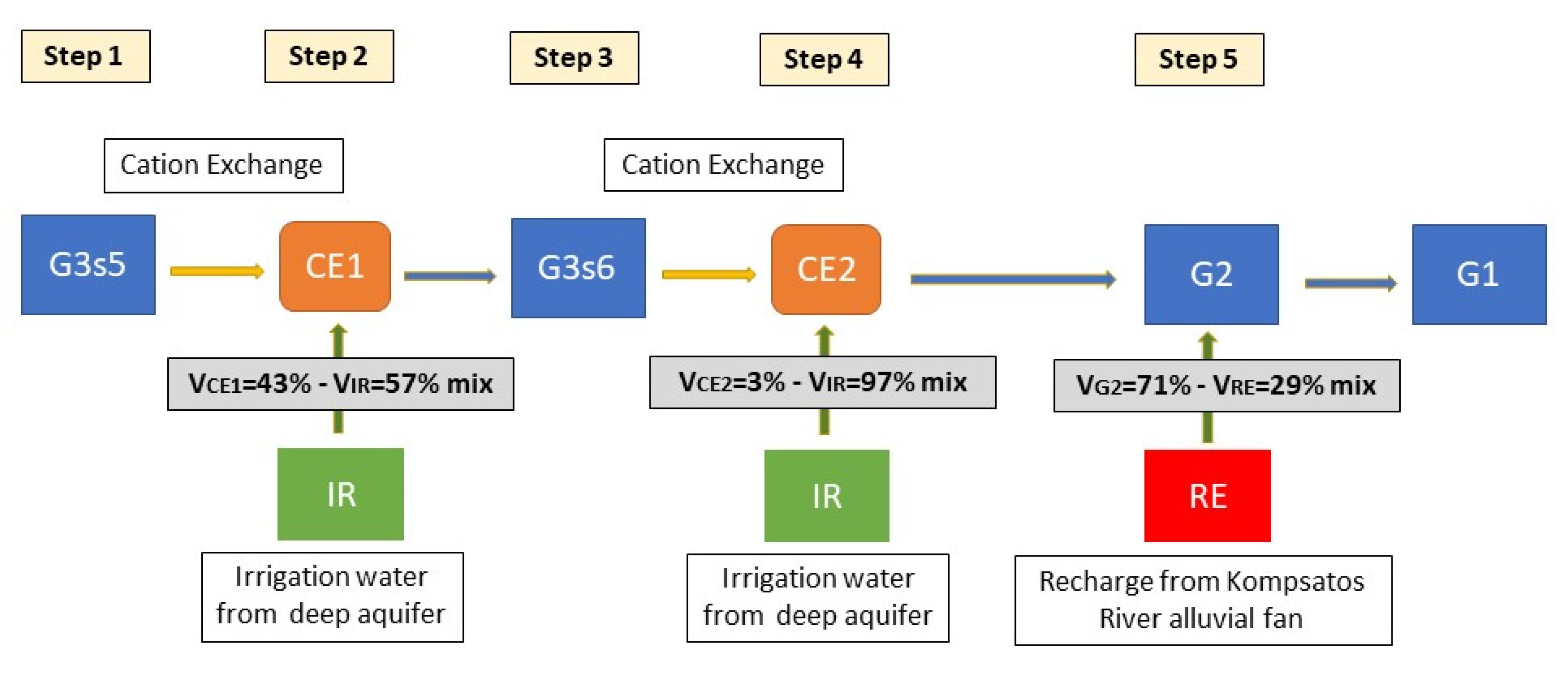
Similar to P1, the model for P2 (Figure 5) consists of five sequential steps. The target is again to model the cation exchange process and to mix samples with the appropriate volumes to obtain a sample which chemistry is as close to G1 as possible. The concentrations of the selected parameters for the samples used are shown in Table 2.

Step 1: The G3s5 sample is submitted to cation exchange (CE1) with similar conditions to P1 (e.g., reactants and constraints). After the model run, we obtain the sample CE1, which chemistry is shown in Table 2.

Step 2: The CE1 sample (obtained from step 1) is mixed with IR to obtain G3s6 as an outcome. That is again decided, as we need freshwater input to reduce the chemical concentrations of CE1 and reach G3s6. The precipitation input is not included due to the reasons described in P1. Applying Equation (1) (C_CE1 ∗ V_CE1 + C_IR ∗ V_IR = C_mix ∗ V_{mix (=1)}) and following the aforementioned process, the concentrations of the key parameters for the targeted mix sample C_G3s6 are better approached when the two volumes are mixed as V_CE1 = 43% and V_IR = 57%.

Step 3: The G3s6 sample is submitted to cation exchange (CE2) with similar conditions to P1 (e.g., reactants and constraints). After the model run, we obtain the sample CE2, which chemistry is shown in Table 2.

Step 4: The CE2 sample (obtained from step 3) is mixed with the IR to obtain G2 as an outcome. By applying Equation (1) (C_CE2 ∗ V_CE2 + C_IR ∗ V_IR = C_mix ∗ V_{mix (=1)}), the targeted mix sample C_G2 is better approached when the two volumes are mixed as V_CE2 = 3% and V_IR = 97%.

Step 5: As reported, the G2 sample receives an amount of freshwater from the recharge of the Kompsatos River alluvial fan. We hypothesize that this water is also mixed with G2, following the mixing of CE2 with the IR. By applying Equation (1) (C_G2 ∗ V_RE + C_G2 ∗ V_RE = C_mix ∗ V_{mix (=1)}), the concentrations of the targeted mix sample C_G1 are better approached when the two volumes are mixed as V_G2 = 71% and V_RE = 29%.

4.3. Conceptualization of Rhodope Aquifer Evolution

The cation exchange has been successfully verified as a dominant process that affects groundwater chemistry and is embedded in the overall groundwater evolution for the Rhodope coastal aquifer. Based on the results of the two models, it is evident that, in the second period (P2—end of the irrigation period), the contribution of the deeper aquifer to the bulk sample of the irrigation boreholes is greater than in the P1. This is significantly evident in step 4 of the P2, where nearly all the exploited groundwater derives from the deeper confined aquifer, and to a lesser extent in step 2. This result is in accordance with the evidence obtained from hydrogeological and hydrogeochemical data as well as from field measurements of electrical conductivity (unpublished data), where the median value for SPC is reduced by nearly 100% (dropping from 2.100μS/cm to roughly 1.050 μS/cm from P1 to P2 for the G2 to which the abovementioned impact is mainly imposed).

Bearing in mind the above, we may assume that, at the beginning of the irrigation period (May) for the coastal Rhodope area, the semi-confined aquifer of low quality (elevated salinization and nitrate content) is the main aquifer system used for irrigation. Progressively during the irrigation period, the upper aquifer is practically depleted. At the end of the irrigation period (late August–early September), the exploitation of the deeper aquifer drastically increases. This fact is evident in the significant improvement of groundwater quality for many of the boreholes in the area. The examined conceptual models for P1 and P2 can verify the above scenario.

4.4. Constraints and Limitations

The proposed modelling approach constitutes a preliminary method for assessing possible groundwater evolution scenarios. In most cases, the common software that can mix two or more solutions (surface or water samples) needs to define a priori the mixing ratios of the initial samples. However, this requires more detailed knowledge of the hydrogeological conditions, or it could be time consuming to use a trial-and-error approach to obtain the initial volumes. That could potentially lead to biased and erroneous results if the initial hypothesis (proportion of mixing) is wrong. The proposed method has the inherent advantage that it does not hypothesize the mixing volumes. Still, it uses simple yet reliable mathematical calculations to reach the smallest deviations (in terms of hydrogeochemistry of selected parameters) from the final target sample.

Nevertheless, this exploratory procedure must be considered in conjunction with specific hydrogeological and hydrogeochemical knowledge. The described modelling process assumes a semi-conservative approach (only key processes related to hydrogeochemistry and not the entire extent of them), where a specific process (e.g., cation exchange) may (or may not, per case) occur during the evolution scenario. The complexity of nature (e.g., several processes with a synergetic or an antagonistic character) are out of the scope of this approach. A careful selection should also be considered in selecting the key parameters that will be evolved in the model. The criteria presented (e.g., key parameters of dominant processes and conservative elements) are indicative and representative of specific case studies. However, the proper selection of the key parameters is a matter of expert judgement and knowledge of site-specific conditions.

4.5. Exploitable Outcomes of the Proposed Method

The proposed methodological approach provides an efficient preliminary tool for assessing groundwater evolution and hydrogeochemical fingerprint. It aims to identify the critical hydrogeological/hydrogeochemical components, for example, the mixing ratios of different water bodies and the derived groundwater chemistry, which are crucial (a) for the development of more sophisticated tools and models that require human and/or financial resources, and (b) to comprehend the basic prerequisites needed for the application of adaptation and/or mitigation measures related to groundwater management. That eventually is expected to significantly impact local societies, considering the critical role of freshwater resources in coastal environments.

As seen in

Table 3. Comparison of previous methods used in literature and the proposed method.

Methods	Tools/Parameters Needed	References
Hydrogeochemical modelling and data analysis	Hydrochemical analysis Mineralogical (main) composition of aquifer matrix Hydrogeochemical modelling (e.g., PHREEQC or GWB softwares) Microsoft xls solver	Propose method in this study
Hydrogeochemical evaluations	Hydrochemical analysis Hydrogeochemical plots (ionic ratio plots and Piper, Gibbs, Wilcox, and van Wirdum diagrams) Water types and hydrochemical facies Water quality indices Spatial interpolation and choropleth maps (GIS) MVSA (Q-mode and R-mode) Saturation indices (PHREEQC) Partial least squares regression model (PLSR)	[1,2,3,4,5,6]
Groundwater Modelling	Hydraulic conductivity, porosity, specific yield, precipitation, groundwater head, and TDS FEFLOW, MODFLOW-2000, and MT3DMS	[7,8,9]
Hydrogeochemical modelling (inverse/forwarding)	Hydrochemical analysis and hydrogeochemical plots (ionic ratio plots, and Piper and Gibbs diagrams) Saturation indices Hydrogeological conceptual model Mixing fractions Virtual samples (VISHMOD model) Geochemical modeling (PHREEQC and MIN3P)	[10,11,12,13]
MVSA	Hydrochemical data Hydrogeochemical tools (ion plots, hydrochemical facies evolution diagram (HFE-D), Gibbs diagram, Wilcox diagram, USSL diagram, and boxplots, with water quality indices) Spatial distribution (ArcGIS) Hierarchical cluster analysis (HCA), principal component analysis (PCA) analysis, and correlation analysis Couple MVSA with multiple linear regression model, and Bregman block average algorithm (BBAC_I)	[14,15,16,18]
Environmental isotopes	Hydrochemical data and tools (ionic sequence, ion plots, and Piper, Schoeller, and Durov diagrams) Spatial distribution (ArcGIS) Determine Local Meteoric Water Line (LMWL), deuterium excess, and water types Coupled with hydrochemical modelling (PHREEQC), MVSA, and groundwater quality index	[19,20,21,22]
Mixing cell model (MCM)	Hydrochemical and isotopic analysis M3 model (multivariate mixing and mass-balance calculations) MVSA (PCA) Couple inverse and forward MCM with groundwater modelling Incorporation of 14C residence time	[23,24]
Classic hydrogeological approaches	Coupling of the aforementioned methods (e.g., coupling of hydrodynamics, hydrochemistry, and environmental isotopes with PCA) Artificial intelligence (AΙ) model	[25,26,27]

, the requirements for applying the proposed method in terms of parameters/tools are less than those required in similar methodological approaches. This poses a significant advantage regarding ease of application and resources needed and demonstrates that the proposed methodology could be used successfully as a preliminary assessment tool.

The impacts of the proposed method’s outcomes depend on the survey’s scale and the available data. Thus, it can be applied to assess the local conditions of a sub-catchment, such as in the case of the Rhodope coastal aquifer. It could be further expanded to cover a regional scale and provide strategic information to key stakeholders and decision makers. Nevertheless, knowledge of key hydrogeological conditions (e.g., hydraulic connections) is always essential to support meaningful and reliable results. Upscaling the proposed method to a larger extent could be possible but needs to be approached with caution, as different and often diverse water bodies are engaged.

Applying a preliminary assessment method such as the one proposed could benefit decision makers and stakeholders, as they save time and resources for more sophisticated approaches. Its outcomes could be validated by managerial plans that are tailored to the specific conditions drawn from the analysis. Eventually, that could lead to a long-term positive impact on an area’s natural environment and socio-economic structure.

5. Conclusions

The two model scenarios for the coastal Rhodope area aquifer system were successfully applied with a combined approach of hydrogeochemical modelling and data analysis for mixing volume optimization. The applied methodology proved to be an efficient preliminary tool for assessing groundwater evolution and hydrogeochemical fingerprint, especially in complex groundwater systems. Its requirements are less than those used in previously applied methods of similar scientific problems, which makes it more attractive and easier to use in cases of limited resources. The results revealed that the evolution of the groundwater system between the start and the end of the irrigation period, which is reflected in the mixing ratios between the upper and the lower aquifer systems and the other reference samples, is temporally dependent. Specifically, the upper aquifer is subjected to cation exchange with significant calcium elevation in the aquatic solution in both periods. The evolution of groundwater from the coastal area towards the inland is performed by mixing the two aquifer layers with different proportions (volumes). The mixing ratio progressively changes following the depletion of the upper semi-confined aquifer. Specifically, the aquifer system is confirmed to undergo cation exchange as the dominant geochemical process that increases calcium concentrations. The complex hydrogeological regime is further evaluated by assessing the mixing ratios of the different aquifer layers. Hence, the aquifer system (bulk samples) is mixed with the irrigation water by 71% and 97% and with the lateral recharge by 76% and 29% for the beginning and the end of the irrigation period, respectively. Overall, this methodological approach may be used as an exploratory and preliminary assessment tool to capture the temporal dynamics in complex groundwater systems and support groundwater resource management. Future improvements should be considered, such as optimizing the mixing ratios of more than two solutions and/or including additional geochemical processes (other than cation exchange) in the hydrogeochemical modelling. Nevertheless, the trade-off between the ease of its applicability and the increased complexity (and requirements) that these modifications might bring should be considered.