Characterization of Sub-Catchment Stream and Shallow Groundwater Nutrients and Suspended Sediment in a Mixed Land Use, Agro-Forested Watershed

Abstract

Excess nutrients and suspended sediment exports from agricultural watersheds are significant sources of global water quality degradation. An improved understanding of surface water and groundwater pollutant loads is needed to advance practices and policies. A study was conducted in an agricultural-forested catchment of the mid-Atlantic region of the United States. Stream water (SW) and shallow groundwater (SGW) samples were collected monthly between January 2020 and December 2021 from eight sub-catchment study sites. Samples were analyzed for nitrate (NO₃-N), nitrite (NO₂-N), total ammonia (NH₃-N), total nitrogen (TN-N), orthophosphate (PO₄³-P), and total phosphate (TP-P) concentrations using spectrophotometric methods. Total suspended solids concentrations (mg/L) were quantified gravimetrically and volumetrically to estimate mean particle diameter (MZ, µm), particle surface area (CS, m²/mL), sample skewness (Ski), and particle size distributions (sand/silt/clay%). Results showed significant (p < 0.05) differences in nutrient concentrations and suspended sediment characteristics between SW and SGW between study sites. Differences were attributed to source water type and sub-watershed location. Principal components analysis indicated seasonal effects on water quality in summer months and connected land use with TSS, TN-N, and TP-P concentrations. Study results emphasize the importance of SGW water quality metrics for non-point source loading predictions to inform management decisions in agro-forested watersheds.

1. Introduction

While nutrients and sediment are naturally occurring components of aquatic ecosystems, excess nitrogen, phosphorus, and suspended sediment can negatively impact environmental waters and their surrounding ecosystems [1,2]. This understanding is essential because concentrations and fluxes of riverine pollutants have been increasing globally [3,4]. For example, Vilmin et al. [5] showed that together with a global increase in riverine nutrient delivery, the proportion of total inorganic nitrogen and phosphorous inputs rose from 30 to 40% and 56 to 65%, respectively, during the 20th century. Furthermore, the transfer of mineral nitrogen and phosphorus from the atmosphere and localized formations to global agricultural soils, along with accelerated urbanization, and increasing wastewater emissions, have amplified and accelerated contemporary surface water nutrient loading [5,6].

Relative to the pre-industrial era, estimates of global riverine flux of total nitrogen have more than doubled due to anthropogenic activities, which include industrial fertilizer application and fixation, livestock production, the harvest and transport of feed and forage for livestock, and sewage disposal [7,8]. Increased nitrogen flux was linked to eutrophication and biodiversity loss in sensitive estuarine waters [9,10]. However, eutrophication is not limited to coastal environments, as riverine environments and their connected floodplains are also at risk of degradation from excess nitrogen inputs [11,12,13].

Globally, riverine suspended sediment increases have been linked to land use changes, including crop farming and deforestation [14,15]. Zeiger and Hubbart [16] modeled suspended sediment loading regimes from pre-development and contemporary periods. They found maximum daily suspended sediment yields (loads per unit area) increased from 35.7 to 59.6 Mg km² in a Central USA mixed land use watershed. In general, increased suspended sediment loading has been attributed to urbanization and the conversion of natural landscapes for farming [17,18]. Excessive suspended sediment loading is also associated with increases in the global riverine flux of particulate nutrients [19,20,21]. For example, increased erosion and high precipitation/flow events are linked with the release of legacy phosphorus to surface and subsurface flow pathways [22,23,24]. Given the historical context, it is reasonable to expect that continued landscape alterations will lead to increased suspended sediment and global nutrient exports for the foreseeable future.

Previous studies showed that agricultural land use correlates with excessive nutrient and suspended sediment exports globally [25,26,27,28]. Impacts due to agricultural land use practices may be important since the world population is expected to increase beyond 9 billion by 2050, adding pressure to the current global food demand and requiring further expansion of agricultural areas [29,30]. Currently, agricultural practices are not on track to meet growing consumption and food demands, which may result in further intensification of contemporary farming practices [31,32], including ongoing degraded soils and non-point pollutant loading [33], and long-lasting effects on aquatic ecosystem health [34] to meet demand. Despite science-based progress, there remains limited information regarding pollutant loading contributions from stream water (SW) and shallow groundwater (SGW) in sub-catchments where agricultural land use contributes to poor downstream water quality [4,9,35]. Previous studies showed that excess nutrients and suspended sediments associated with agricultural land uses are often delivered to water bodies via surface pathways [36,37,38]. However, recent studies have demonstrated the importance of subsurface pathways as delivery mechanisms for suspended sediments and particulate nutrients [39,40,41,42], thus signifying the need for further non-point pollutant characterization in SW and SGW from agricultural watersheds.

In the mid-Atlantic region of the USA, agricultural land use comprises approximately 26–29% of the Chesapeake Bay Watershed (CBW) and is a significant source of excess nutrients and suspended sediments, contributing to estuarine biological impairment and poor water quality throughout the region [43,44,45,46]. The CBW represents many managed, diverse temperate landscapes that support agricultural land uses globally [2,47]. Although total nitrogen loads in the CBW have decreased since the late 1980s, partly due to the implementation of the total daily maximum daily nutrient loading (TMDL) goals, total phosphorus and suspended sediment loads have increased since the mid-1990s [48,49,50]. Recent (i.e., 2009–2018) estimates from the Chesapeake Bay nontidal network (NTN) showed that total nitrogen loading was improving at 41% of the NTN stations, total phosphorus loading was improving at 44% of the NTN stations, and suspended sediment loading was degrading (i.e., increasing) at 42% of the NTN stations [51,52]. These mixed results show room to advance non-point source pollutant reduction strategies in the CBW. For example, agriculturally sourced phosphorus and suspended sediment loading estimates could be improved by monitoring SW and SGW quality in CBW headwater regions [53]. Given the continued non-point source pollutant problems in the CBW, better characterization of SW and SGW nutrients and suspended sediment loads in smaller agricultural catchments can improve downstream water quality predictions and help assess if TMDL goals will be achieved [54].

Understanding the relationships between excess nutrients and suspended sediment loading with land use has advanced in recent years [24,55,56,57,58], which has helped inform pollutant reduction strategies worldwide [17,59]. However, phosphorus and suspended sediment loads are still increasing in many sub-catchments [60]. Therefore, further study is needed, particularly in regions where agricultural land use contributes to pollutant loading via surface and subsurface pathways [23,61]. Additional contemporaneous information may better drive management practices and policies. Therefore, the objectives of the current work were to (a) characterize SW and SGW nutrient (i.e., nitrogen and phosphorus) concentrations and suspended sediment characteristics in a contemporary agricultural (agro) and forested watershed and (b) evaluate the use of monthly sub-catchment sampling to summarize nutrient and suspended sediment patterns. The current work’s results can guide management practice decisions to improve water quality in small, agro-forested watersheds.

2. Materials and Methods

2.1. Study Site Description

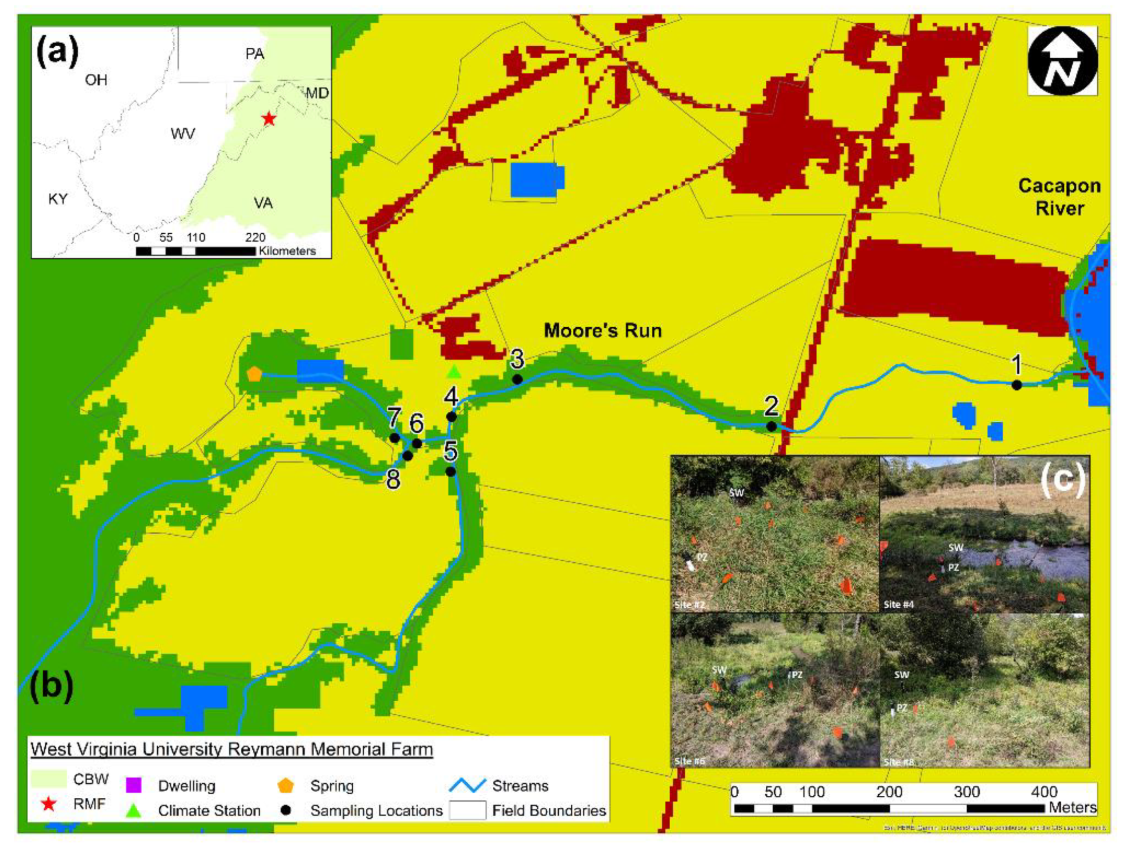
The current work was conducted in Moore’s Run Watershed, a 36 km² mixed land use, agro-forested watershed located in Hampshire and Hardy counties, West Virginia, USA (Figure 1). Moore’s Run is a tributary of the Cacapon River, a CBW headwater catchment that flows through Reymann Memorial Farm (39°6′12.73″ N, 78°35′8.19″ W). Although much of Moore’s Run Watershed is forested, the downstream stream corridor is primarily agricultural and lacks a forested buffer (Figure 1). Land use in Moore’s Run Watershed is approximately 87% forest, 11% agriculture, and 2% developed (

Table 1. Land use/land cover characteristics (% cover) and total drainage area (km²) at eight sub-basin monitoring sites comprising an experimental watershed study in Moore’s Run Watershed, WV, USA.

Site	Forest (%)	Agriculture (%)	Developed (%)	Drainage Area (km2)
1	86.5	10.5	2.0	35.5
2	88.3	8.8	1.9	34.6
3	88.3	8.8	1.9	34.5
4	88.3	8.8	1.9	34.5
5	88.5	8.5	1.9	33.7
6	79.2	20.3	0.2	0.8
7	57.2	42.8	0.0	<0.1
8	83.4	16.3	0.3	0.5

). The forest comprises dry-mesic oak forests, dry calcareous forests, and other mixed forest assemblages, while the agricultural areas consist of low vegetation, hay/pasture, and cultivated crops [62]. Reymann Memorial Farm was historically used for beef cattle production and is currently operated by West Virginia University as a working farm used for research on livestock feed and environmental quality [63,64].

Moore’s Run Watershed geology comprises sandstone, shale, and alluvium. Study sites were installed on either alluvial or shale deposits [65]. Soils in the watershed consist of moderately-drained Basher fine sandy loam in the floodplains and Monongahela silt loam (3–8% slopes) along stream terraces [66]. Average (n = 179 and total core number per site, n = 14–27) soil dry bulk density and porosity at the study sites range from 1.03 to 1.30 g cm³ and 0.51–0.61, respectively, while average (n = 6, slug tests per site) saturated hydraulic conductivity (K_sat) ranges from 0.29 to 4.76 m day⁻¹ [67]. Long-term average annual (1917–2016) air temperature, precipitation, and total snowfall at Reymann Memorial Farm were 8.7 °C, 811 mm, and 511 mm, respectively [68].

2.2. Nutrient and Suspended Sediment Data Collection

Eight study sites were established at Reymann Memorial Farm in 2019 using a nested-scale experimental watershed study design [58,69,70], which is an effective and customizable study design that has been used to characterize the effects of land use changes on water quality and quantity for well over a century [70,71,72,73,74]. A single representative climate station was installed on a relatively flat/open area near Site #4 (Figure 1). Monitored climate variables included air temperature and precipitation [75]. All climate variables were sensed at 30 min intervals, and the total rainfall was recorded with a Texas Instruments tipping bucket rain gauge (Campbell Scientific Inc., Logan, UT, USA).

Each sub-watershed outlet (n = 8; Figure 1) was instrumented with a co-located polyvinyl chloride (PVC) stilling well (3.2 cm inner diameter) and steel drive point piezometer (3.2 cm inner diameter, screened for the bottom 76.5 cm with 1 cm slotted pipe and 0.03 cm diameter mesh screen) to monitor stream water (SW) stage and shallow groundwater (SGW) stage in the unconfined alluvial aquifer, respectively. Piezometer depths ranged from 0.98 to 2.01 m and were driven to a depth of approximately 0.50 m below the adjacent streambed. Distance between stilling wells and piezometers ranged from 1.3 to 17.8 m at each study site.

Evaluation of SW and SGW nutrient concentrations and suspended sediment characteristics included a monthly sampling campaign (January 2020–December 2021), during which 1 L grab samples were collected from stilling well study site (n = 8) locations and 1 L samples were pumped from piezometers (n = 8). Samples were collected on the third Wednesday of each month (between 8:00 h and 12:00 h) for the duration of the study period. Samples were always collected from sites in reverse sequential order (i.e., Site #8 – Site #1), and SW was always sampled before the SGW. SW samples were collected within 1 m of each stilling well and from 60% of stream depth [24]. SGW samples were collected with a Masterflex E/S Portable Sampler peristaltic pump (Cole Parmer; Vernon Hills, IL, USA). SGW was pumped from the piezometers through size 15 tubing at a rate of 17 mL s⁻¹. Piezometers were purged and allowed to refill before SGW sample collection.

After each grab sample collection, 50 mL aliquots were filtered in the field using a 0.45 µm syringe filter and preserved for future nutrient analyses [76]. Filtered samples were fixed with a 2 mL nitric acid (concentration ~ 8%) addition. Filtered/fixed aliquots and the remaining grab sample portions (i.e., ~0.95 L unfiltered samples) were stored in an insulated cooler, delivered to the laboratory within seven hours of collection, and refrigerated at 2 °C until analysis. The filtered/fixed samples were analyzed for nutrient concentrations within 24 h of collection. The remaining grab samples were analyzed for total suspended solids (TSS; mg L⁻¹) within one week of collection [77]. Additional suspended sediment characteristics [i.e., mean particle size (MZ; µm), calculated surface area (CS; m² mL⁻¹), skewness (Ski), and sand/silt/clay percentages (%)] were determined within 28 days of collection [78]. Nutrient analyses were conducted using a HACH DR 3800 spectrophotometer (HACH Company; Loveland, CO, USA). Nutrient concentrations, including nitrate (NO₃-N), nitrite (NO₂-N), total ammonia (NH₃-N), total nitrogen (TN-N), orthophosphate (PO₄³-P), and total phosphate (TP-P), were quantified spectrophotometrically with HACH TNTPlus^TM analytes (Hach Company, Loveland, CO, USA). Nutrient standards were run with a 3% tolerance of error [28]. TSS was determined from secondary grab sample aliquots (i.e., 37–300 mL) using established gravimetric filtration methods [79].

Additional grab sample aliquots (i.e., 200 mL) were analyzed with a Microtrac BLUEWAVE Laser Diffraction analyzer (Microtrac, York, PA, USA) [80,81,82]. Laser particle diffraction results included mean particle diameter (MZ, µm), calculated particle surface area (CS, m²/mL), sample skewness (Ski), and particle size distributions that were binned by size class into sand/silt/clay fractions (%). For additional details on the methods used for the laser particle diffraction analysis, please see Gootman and Hubbart [41]. At the time of grab sample collection, a handheld water quality sonde (YSI/Xylem; Yellow Springs, OH, USA), which was calibrated weekly, was used to determine physicochemical variables [i.e., water temperature (Tw; °C), dissolved oxygen (DO; % saturation), specific conductance (SPC; µs cm⁻¹), and pH]. The sonde tip was inserted into the stream to approximately 60% depth so that the data collected represented a representative SW sample [83]. The sonde tip was also immediately inserted into the SGW grab sample bottle to obtain an estimation of the alluvial aquifer physicochemical conditions.

2.3. Data Analyses

Descriptive statistics were generated for study site (n = 8) SW and SGW nutrient concentrations, suspended sediment characteristics, and physicochemical variables. Statistical analyses were conducted using OriginPro 9.6 (OriginLab Corporation, Northampton, MA, USA). All data analyses were performed using established parametric and non-parametric methods [84]. Normality was assessed using the Anderson–Darling test [85]. Aggregated results were characterized by non-normal distributions and required non-parametric testing methods [86]. Friedman’s ANOVA [87] was used for inter-site SW and SGW result comparisons. A Spearman’s correlation test [88] was used to quantify relationships between nutrient concentrations, suspended sediment characteristics, physicochemical variables, and sub-watershed land use. Relationships between nutrient concentrations, suspended sediment characteristics, physicochemical data, and sub-watershed land use were characterized with a principal components analysis (PCA) to determine factors driving the observed water quality parameter behavior(s) [76,89,90,91]. Biplots generated to visualize PCA results were similar to correlation biplots; however, OriginPro does not scale loadings, since scores are standardized, and loadings and scores are provided separate axes in biplots [76]. The significance threshold for all statistical tests was α = 0.05.

3. Results

3.1. Climate during Study

Moore’s Run Watershed received approximately 19% more total precipitation in 2020 (961.5 mm) and 14% more total rainfall in 2021 (923.8 mm) than the long-term (1917–2016) annual average (811 mm) [68]. In 2020, September was the driest (41.9 mm) month, and April was the wettest (128.5 mm) month. In 2021, December was the driest (18.1 mm) month, and August was the wettest (154.3 mm) month. Average annual air temperatures in 2020 (13.09 °C) and 2021 (11.15 °C) were higher than the long-term (1917–2016) annual average air temperature (8.7 °C) [68]. Compared to long-term annual averages, these climatic results reflect how the West Virginia climate is becoming increasingly temperate [92,93].

3.2. Nutrient Concentrations

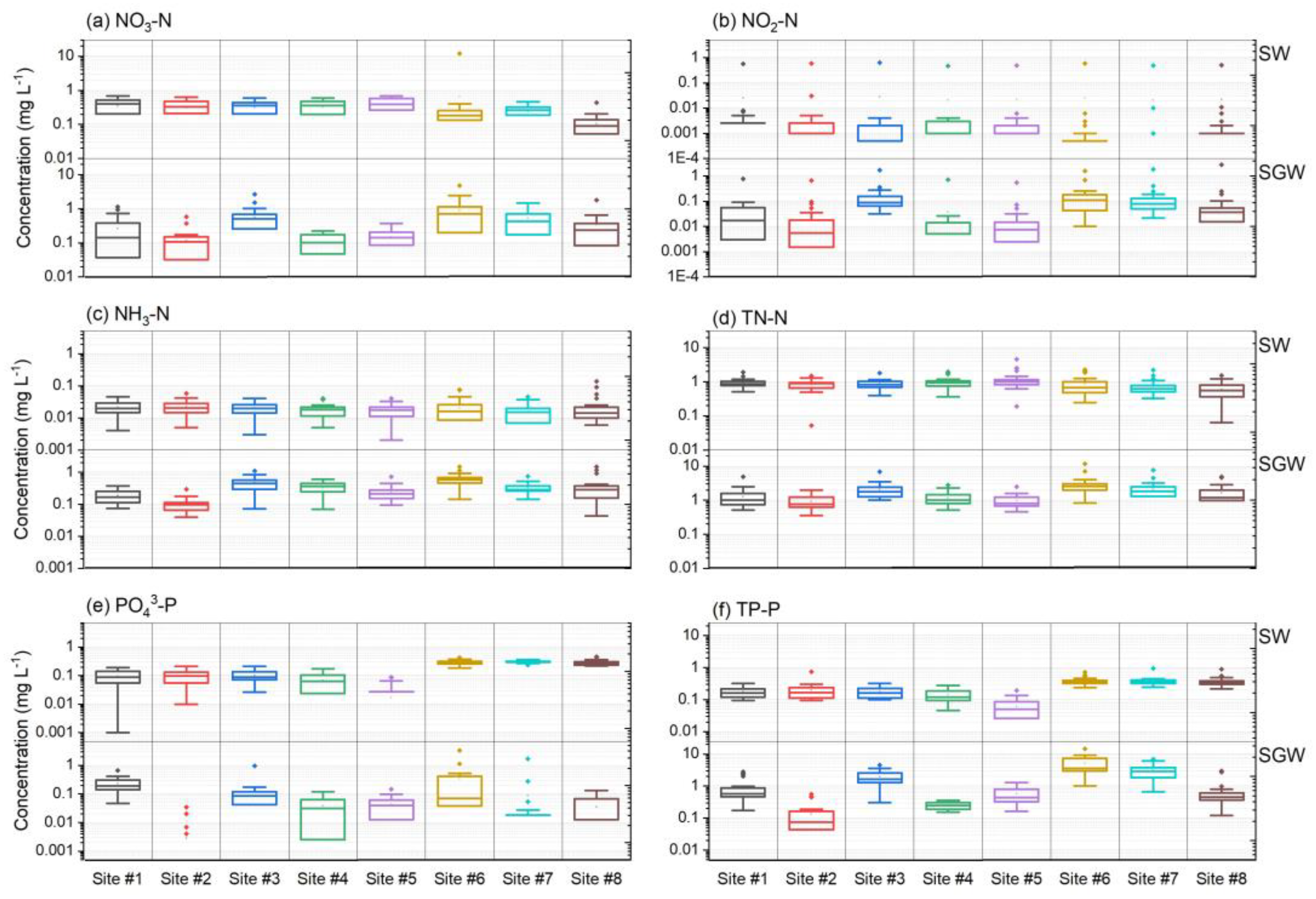
Observed nutrient concentrations (NO₃-N, NO₂-N, NH₃-N, TN-N, PO₄³-P, and TP-P; Figure 2) indicated distinct water source and spatial patterns for Moore’s Run Watershed surface water (SW;

Table 2. Average values (with standard deviations in parentheses) for nutrient concentrations (mg L⁻¹), suspended sediment characteristics [total suspended solids; TSS (mg L⁻¹), mean particle size; MZ (µm), calculated surface area; CS (m² mL⁻¹), skewness; Ski, Sand (%), Silt (%), and Clay (%)], and physicochemical variables [water temperature (Tw; °C), dissolved oxygen (DO;% saturation), specific conductance (SPC; µs cm⁻¹), and pH] of surface water (SW) during the study period (January 2020–December 2021) for eight monitoring sites in Moore’s Run, Watershed, WV, USA.

SW	Site #1	Site #2	Site #3	Site #4
NO3-N	0.34 (0.21)	0.32 (0.19)	0.32 (0.19)	0.33 (0.19)
NO2-N	0.03 (0.12)	0.03 (0.12)	0.03 (0.13)	0.02 (0.09)
NH3-N	0.02 (0.01)	0.02 (0.01)	0.02 (0.01)	0.02 (0.01)
TN-N	0.93 (0.29)	0.84 (0.29)	0.86 (0.29)	0.99 (0.42)
PO43-P	0.09 (0.06)	0.10 (0.06)	0.10 (0.05)	0.07 (0.05)
TP-P	0.18 (0.07)	0.20 (0.14)	0.18 (0.07)	0.14 (0.06)
TSS	8.46 (9.25)	11.26 (21.31)	9.52 (11.03)	9.42 (6.61)
MZ	41.18 (14.72)	52.81 (71.61)	43.05 (13.05)	68.48 (128.47)
CS	0.56 (0.20)	0.67 (0.40)	0.53 (0.17)	0.49 (0.16)
Ski	0.47 (0.18)	0.53 (0.13)	0.53 (0.12)	0.43 (0.26)
Sand	28.12 (11.65)	28.44 (10.55)	29.94 (8.17)	32.06 (13.26)
Silt	63.78 (9.72)	62.72 (9.20)	62.33 (8.11)	61.11 (11.39)
Clay	8.10 (3.83)	8.84 (4.85)	7.74 (3.63)	6.83 (3.07)
Tw	11.85 (5.38)	11.64 (5.21)	11.49 (5.06)	10.95 (5.54)
DO	102.61 (4.97)	102.67 (4.67)	98.30 (14.53)	100.43 (3.27)
SPC	225.74 (19.65)	221.86 (19.51)	222.10 (19.64)	228.89 (21.00)
pH	8.17 (0.24)	8.21 (0.22)	8.13 (0.21)	8.14 (0.21)
SW	Site #5	Site #6	Site #7	Site #8
NO3-N	0.38 (0.23)	0.67 (2.44)	0.23 (0.13)	0.10 (0.09)
NO2-N	0.02 (0.10)	0.02 (0.12)	0.02 (0.10)	0.02 (0.10)
NH3-N	0.02 (0.01)	0.02 (0.02)	0.02 (0.01)	0.02 (0.03)
TN-N	1.25 (0.90)	0.88 (0.58)	0.73 (0.43)	0.60 (0.35)
PO43-P	0.02 (0.03)	0.29 (0.05)	0.30 (0.03)	0.28 (0.06)
TP-P	0.06 (0.05)	0.38 (0.11)	0.39 (0.13)	0.36 (0.14)
TSS	8.35 (9.38)	16.28 (13.84)	23.50 (43.14)	9.26 (11.39)
MZ	48.67 (23.53)	55.34 (26.09)	49.31 (12.68)	184.71 (383.01)
CS	0.72 (0.50)	0.43 (0.13)	0.40 (0.12)	0.45 (0.35)
Ski	0.40 (0.25)	0.53 (0.18)	0.47 (0.19)	0.41 (0.28)
Sand	34.02 (13.19)	35.58 (9.99)	34.92 (10.64)	40.92 (22.17)
Silt	57.75 (11.96)	58.68 (10.17)	59.89 (10.28)	53.03 (20.24)
Clay	8.23 (3.52)	5.74 (2.71)	5.19 (2.63)	6.04 (5.25)
Tw	10.65 (6.22)	11.99 (2.71)	12.72 (1.84)	10.95 (3.78)
DO	101.25 (3.09)	92.93 (6.42)	89.15 (5.15)	95.50 (5.04)
SPC	244.87 (30.38)	183.36 (12.29)	182.68 (11.50)	185.04 (13.15)
pH	8.14 (0.23)	7.65 (0.24)	7.58 (0.17)	7.52 (0.29)

) and shallow groundwater (SGW;

Table 3. Average values (with standard deviations in parentheses) for nutrient concentrations (mg L⁻¹), suspended sediment characteristics [total suspended solids; TSS (mg L⁻¹), mean particle size; MZ (µm), calculated surface area; CS (m² mL⁻¹), skewness; Ski, Sand (%), Silt (%), and Clay (%)], and physicochemical variables [water temperature (Tw; °C), dissolved oxygen (DO;% saturation), specific conductance (SPC; µs cm⁻¹), and pH] of shallow groundwater (SGW) during the study period (January 2020–December 2021) for eight monitoring sites in Moore’s Run, Watershed, WV, USA.

SGW	Site #1	Site #2	Site #3	Site #4
NO3-N	0.26 (0.31)	0.12 (0.13)	0.57 (0.58)	0.10 (0.07)
NO2-N	0.06 (0.16)	0.04 (0.14)	0.19 (0.34)	0.04 (0.14)
NH3-N	0.19 (0.09)	0.10 (0.06)	0.47 (0.24)	0.34 (0.15)
TN-N	1.27 (0.90)	0.93 (0.48)	2.03 (1.25)	1.17 (0.54)
PO43-P	0.23 (0.14)	0.00 (0.01)	0.12 (0.19)	0.04 (0.04)
TP-P	0.86 (0.74)	0.13 (0.15)	1.97 (0.98)	0.25 (0.07)
TSS	104.95 (144.77)	87.48 (108.00)	407.75 (357.51)	32.78 (23.97)
MZ	21.61 (6.07)	37.84 (69.41)	13.20 (2.39)	85.88 (85.98)
CS	1.71 (0.98)	1.17 (0.29)	1.69 (0.60)	1.17 (0.77)
Ski	0.70 (0.11)	0.68 (0.11)	0.61 (0.03)	0.65 (0.25)
Sand	14.48 (5.19)	15.52 (7.08)	6.35 (2.29)	33.56 (21.30)
Silt	63.81 (8.72)	65.76 (7.64)	67.15 (3.85)	51.30 (15.49)
Clay	21.72 (8.25)	18.73 (4.26)	26.50 (4.27)	15.14 (10.25)
Tw	12.31 (4.24)	13.65 (5.57)	13.14 (4.28)	12.48 (5.45)
DO	22.60 (4.27)	31.87 (4.53)	22.97 (3.67)	25.28 (7.11)
SPC	342.18 (69.46)	362.75 (56.44)	396.00 (45.26)	296.24 (39.47)
pH	6.88 (0.23)	7.17 (0.19)	7.18 (0.20)	7.68 (0.27)
(SGW)	Site #5	Site #6	Site #7	Site #8
NO3-N	0.15 (0.10)	0.89 (1.05)	0.52 (0.44)	0.34 (0.47)
NO2-N	0.04 (0.11)	0.20 (0.33)	0.18 (0.37)	0.17 (0.57)
NH3-N	0.24 (0.14)	0.61 (0.29)	0.33 (0.13)	0.36 (0.35)
TN-N	0.97 (0.46)	3.02 (2.21)	2.12 (1.52)	1.63 (1.12)
PO43-P	0.04 (0.04)	0.34 (0.69)	0.09 (0.35)	0.03 (0.04)
TP-P	0.58 (0.32)	5.18 (3.18)	3.14 (1.77)	0.66 (0.70)
TSS	53.76 (34.68)	477.63 (482.48)	360.18 (403.95)	182.87 (216.46)
MZ	46.60 (126.30)	23.03 (25.08)	22.04 (5.91)	18.09 (10.15)
CS	2.81 (1.77)	2.98 (3.23)	1.21 (0.34)	1.39 (0.44)
Ski	0.64 (0.20)	0.68 (0.07)	0.65 (0.04)	0.66 (0.11)
Sand	13.31 (12.20)	12.78 (6.37)	14.53 (5.28)	10.05 (6.18)
Silt	59.75 (9.82)	63.24 (9.15)	66.61 (5.62)	67.11 (6.09)
Clay	26.94 (9.44)	23.98 (8.87)	18.86 (3.84)	22.85 (7.99)
Tw	12.66 (5.95)	12.37 (5.33)	12.53 (4.86)	12.45 (5.41)
DO	26.00 (6.51)	37.81 (5.93)	45.33 (14.22)	33.69 (7.69)
SPC	304.70 (32.68)	395.26 (177.55)	326.27 (82.23)	363.79 (49.04)
pH	7.31 (0.22)	7.08 (0.23)	7.35 (0.24)	6.95 (0.30)

). SW mean concentrations of NO₂-N, NH₃-N, and TP-P were consistently lower relative to SGW mean concentrations at each study site. Significant differences (p < 0.05) between study sites were identified for every measured nutrient concentration except SW NO₂-N (Appendix A,

Table A1. Results of inter-site comparisons, via Friedman’s ANOVA and Dunn’s post hoc multiple comparison tests, for significant differences (CI = 95%) between surface water nutrient concentrations (mg L⁻¹), suspended sediment characteristics [total suspended solids; TSS (mg L⁻¹), mean particle size; MV (µm), calculated surface area; CS (m² mL⁻¹), skewness; Ski, Sand (%), Silt (%), and Clay (%)], and physicochemical variables [water temperature (Tw; °C), dissolved oxygen (DO;% saturation), specific conductance (SPC; µs cm⁻¹), and pH] at each monitoring site (n = 8) from January 2020–December 2021 measured in Moore’s Run, Watershed, WV, USA. Note: red values indicate significant differences (p < 0.05), and yellow cells indicate significant differences (p < 0.001).

NO3-N (mg L−1)
Site #	1	2	3	4	5	6	7	8
1	1
2	1	1
3	1	1	1
4	1	1	1	1
5	1	0.6	0.56	1	1
6	0.001	0.07	0.08	0.004	0.001	1
7	0.16	1	1	0.82	0.006	1	1
8	0.001	0.001	0.001	0.001	0.001	1	0.05	1
NO2-N (mg L−1)
Site #	1	2	3	4	5	6	7	8
1	1
2	1	1
3	1	1	1
4	1	1	1	1
5	1	1	1	1	1
6	0.95	0.44	1	1	1	1
7	0.19	0.07	0.88	0.45	0.29	1	1
8	1	1	1	1	1	1	1	1
NH3-N (mg L−1)
Site #	1	2	3	4	5	6	7	8
1	1
2	1	1
3	1	1	1
4	0.76	0.65	0.52	1
5	0.76	0.65	0.52	1	1
6	1	1	1	1	1	1
7	0.02	0.01	0.009	1	1	1	1
8	1	1	1	1	1	1	1	1
TN-N (mg L−1)
Site #	1	2	3	4	5	6	7	8
1	1
2	1	1
3	1	1	1
4	1	1	1	1
5	1	0.7	0.16	1	1
6	0.6	1	1	0.44	0.005	1
7	0.07	0.65	1	0.05	0.001	1	1
8	0.001	0.004	0.03	0.001	0.001	0.65	1	1
PO43-P (mg L−1)
Site #	1	2	3	4	5	6	7	8
1	1
2	1	1
3	1	1	1
4	0.44	0.21	0.08	1
5	0.003	0.001	0.001	1	1
6	0.001	0.001	0.002	0.001	0.001	1
7	0.001	0.001	0.001	0.001	0.001	1	1
8	0.002	0.00575	0.02	0.001	0.001	1	1	1
TP-P (mg L−1)
Site #	1	2	3	4	5	6	7	8
1	1
2	1	1
3	1	1	1
4	1	0.82	0.88	1
5	0.008	0.002	0.002	1	1
6	0.001	0.001	0.001	0.001	0.001	1
7	0.001	0.001	0.001	0.001	0.001	1	1
8	0.001	0.006	0.006	0.001	0.001	1	1	1
TSS (mg L−1)
Site #	1	2	3	4	5	6	7	8
1	1
2	1	1
3	1	1	1
4	1	1	1	1
5	1	1	1	1	1
6	0.29	0.7	0.07	1	0.17	1
7	1	1	0.34	1	0.76	1	1
8	1	1	1	1	1	0.21	0.88	1
MZ (µm)
Site #	1	2	3	4	5	6	7	8
1	1
2	1	1
3	1	1	1
4	1	1	1	1
5	1	1	1	1	1
6	0.16	0.002	0.04	1	0.85	1
7	1	0.23	1	1	1	1	1
8	0.85	0.02	0.27	1	1	1	1	1
CS (m2 mL−1)
Site #	1	2	3	4	5	6	7	8
1	1
2	1	1
3	1	0.53	1
4	1	0.05	1	1
5	1	1	1	0.98	1
6	0.04	0.001	0.27	1	0.002	1
7	0.07	0.001	0.45	1	0.005	1	1
8	0.62	0.001	1	1	0.07	1	1	1
Ski
Site #	1	2	3	4	5	6	7	8
1	1
2	1	1
3	1	1	1
4	1	1	1	1
5	1	0.19	1	1	1
6	0.38	1	0.35	0.02	0.001	1
7	1	1	1	1	1	0.02	1
8	1	1	1	1	1	0.1	1	1
Sand (%)
Site #	1	2	3	4	5	6	7	8
1	1
2	1	1
3	1	1	1
4	1	0.35	1	1
5	1	0.32	1	1	1
6	0.29	0.003	0.27	1	1	1
7	1	0.09	1	1	1	1	1
8	0.25	0.002	0.23	1	1	1	1	1
Silt (%)
Site #	1	2	3	4	5	6	7	8
1	1
2	1	1
3	1	1	1
4	1	1	1	1
5	1	0.27	1	1	1
6	0.32	0.05	0.98	1	1	1
7	1	0.62	1	1	1	1	1
8	0.06	0.007	0.23	1	1	1	1	1
Clay (%)
Site #	1	2	3	4	5	6	7	8
1	1
2	1	1
3	1	0.85	1
4	1	0.05	1	1
5	1	1	1	0.49	1
6	0.07	0.001	0.29	1	0.006	1
7	0.04	0.001	0.17	1	0.001	1	1
8	0.35	0.001	1	1	0.013	1	1	1
Tw (°C)
Site #	1	2	3	4	5	6	7	8
1	1
2	1	1
3	0.76	1	1
4	0.002	0.12	1	1
5	0.001	0.06	1	1	1
6	1	1	1	0.82	0.44	1
7	1	1	1	0.05	0.02	1	1
8	0.01	0.44	1	1	1	1	0.19	1
DO (% saturation)
Site #	1	2	3	4	5	6	7	8
1	1
2	1	1
3	1	1	1
4	1	0.38	1	1
5	1	1	1	1	1
6	0.001	0.001	0.001	0.001	0.001	1
7	0.001	0.001	0.001	0.001	0.001	1	1
8	0.001	0.001	0.04	0.34	0.009	1	0.09	1
SPC (µs cm−1)
Site #	1	2	3	4	5	6	7	8
1	1
2	0.27	1
3	0.7	1	1
4	1	0.05	0.16	1
5	0.7	0.001	0.001	1	1
6	0.001	0.009	0.002	0.001	0.001	1
7	0.001	0.001	0.001	0.001	0.001	1	1
8	0.001	0.1572	0.05	0.001	0.001	1	1	1
pH
Site #	1	2	3	4	5	6	7	8
1	1
2	1	1
3	1	0.48	1
4	1	1	1	1
5	1	1	1	1	1
6	0.001	0.001	0.001	0.001	0.001	1
7	0.001	0.001	0.001	0.001	0.001	1	1
8	0.001	0.001	0.001	0.001	0.001	1	1	1

;

Table A2. Results of inter-site comparisons, via Friedman’s ANOVA and Dunn’s post hoc multiple comparison tests, for significant differences (CI = 95%) between shallow groundwater nutrient concentrations (mg L⁻¹), suspended sediment characteristics [total suspended solids; TSS (mg L⁻¹), mean particle size; MZ (µm), calculated surface area; CS (m² mL⁻¹), skewness; Ski, Sand (%), Silt (%), and Clay (%)], and physicochemical variables [water temperature (Tw; °C), dissolved oxygen (DO;% saturation), specific conductance (SPC; µs cm⁻¹), and pH] at each monitoring site (n = 8) from January 2020–December 2021 measured in Moore’s Run, Watershed, WV, USA. Note: red values indicate significant differences (p < 0.05) and yellow cells indicate significant differences (p < 0.001).

NO3-N (mg L−1)
Site #	1	2	3	4	5	6	7	8
1	1
2	1	1
3	0.06	0.001	1
4	1	1	0.001	1
5	1	1	0.007	1	1
6	0.005	0.001	1	0.001	0.001	1
7	0.13	0.001	1	0.001	0.02	1	1
8	1	0.11	0.82	0.37	1	0.12	1	1
NO2-N (mg L−1)
Site #	1	2	3	4	5	6	7	8
1	1
2	1	1
3	0.001	0.001	1
4	0.95	1	0.001	1
5	1	1	0.001	1	1
6	0.005	0.001	1	0.001	0.001	1
7	0.001	0.001	1	0.001	0.001	1	1
8	1	0.06	0.34	0.004	0.03	1	0.48	1
NH3-N (mg L−1)
Site #	1	2	3	4	5	6	7	8
1	1
2	0.41	1
3	0.001	0.001	1
4	0.1	0.001	1	1
5	1	0.006	0.06	1	1
6	0.001	0.001	1	0.07	0.001	1
7	0.09	0.001	1	1	1	0.08	1
8	0.65	0.001	1	1	1	0.007	1	1
TN-N (mg L−1)
Site #	1	2	3	4	5	6	7	8
1	1
2	1	1
3	0.006	0.001	1
4	1	1	0.01	1
5	1	1	0.001	1	1
6	0.001	0.001	1	0.001	0.001	1
7	0.19	0.001	1	0.34	0.004	0.27	1
8	1	0.04	1	1	0.17	0.006	1	1
PO43-P (mg L−1)
Site #	1	2	3	4	5	6	7	8
1	1
2	0.001	1
3	0.6	0.001	1
4	0.001	0.03	0.65	1
5	0.001	0.02	0.82	1	1
6	1	0.001	1	0.19	0.24	1
7	0.001	1	0.002	1	1	0.001	1
8	0.001	0.24	0.12	1	1	0.02	1	1
TP-P (mg L−1)
Site #	1	2	3	4	5	6	7	8
1	1
2	0.003	1
3	0.16	0.001	1
4	0.09	1	0.001	1
5	1	0.03	0.02	0.52	1
6	0.001	0.001	0.82	0.001	0.001	1
7	0.004	0.001	1	0.001	0.001	1	1
8	1	0.01	0.05	0.27	1	0.001	0.001	1
TSS (mg L−1)
Site #	1	2	3	4	5	6	7	8
1	1
2	1	1
3	0.001	0.001	1
4	0.19	0.7	0.001	1
5	1	1	0.001	1	1
6	0.001	0.001	1	0.001	0.001	1
7	0.001	0.001	1	0.001	0.001	1	1
8	1	0.48	0.44	0.001	0.05	0.17	0.82	1
MZ (µm)
Site #	1	2	3	4	5	6	7	8
1	1
2	1	1
3	0.001	0.001	1
4	0.34	0.95	0.001	1
5	1	1	0.13	0.002	1
6	1	1	0.01	0.03	1	1
7	1	1	0.001	1	1	1	1
8	0.76	0.27	0.95	0.001	1	1	0.17	1
CS (m2 mL−1)
Site #	1	2	3	4	5	6	7	8
1	1
2	1	1
3	1	0.04	1
4	1	1	0.02	1
5	0.19	0.001	1	0.001	1
6	1	0.26661	1	0.16	1	1
7	0.95	1	0.009	1	0.001	0.07	1
8	1	1	1	1	0.07	1	1	1
Ski
Site #	1	2	3	4	5	6	7	8
1	1
2	1	1
3	0.001	0.12	1
4	1	1	0.003	1
5	1	1	0.05	1	1
6	1	1	0.02	1	1	1
7	0.007	1	1	0.19	1	0.7	1
8	1	1	0.13	1	1	1	1	1
Sand (%)
Site #	1	2	3	4	5	6	7	8
1	1
2	1	1
3	0.001	0.001	1
4	1	0.95	0.001	1
5	1	1	0.09	0.005	1
6	1	1	0.03	0.02	1	1
7	1	1	0.001	1	1	1	1
8	0.37	0.52	0.7	0.001	1	1	0.37	1
Silt (%)
Site #	1	2	3	4	5	6	7	8
1	1
2	1	1
3	0.82	1	1
4	0.03	0.001	0.001	1
5	1	0.7	0.01	1	1
6	1	1	1	0.006	1	1
7	1	1	1	0.001	0.04	1	1
8	1	1	1	0.001	0.7	1	1	1
Clay (%)
Site #	1	2	3	4	5	6	7	8
1	1
2	1	1
3	0.11	0.001	1
4	1	1	0.001	1
5	0.52	0.01	1	0.001	1
6	1	1	0.7	0.37	1	1
7	1	1	0.001	1	0.006	1	1
8	1	1	0.32	0.82	1	1	1	1
Tw (°C)
Site #	1	2	3	4	5	6	7	8
1	1
2	0.007	1
3	1	1	1
4	1	0.02	1	1
5	1	0.24	1	1	1
6	1	0.08	1	1	1	1
7	1	0.08	1	1	1	1	1
8	1	0.03	1	1	1	1	1	1
DO (% saturation)
Site #	1	2	3	4	5	6	7	8
1	1
2	0.001	1
3	1	0.001	1
4	1	0.009	1	1
5	1	0.03	1	1	1
6	0.001	1	0.001	0.001	0.001	1
7	0.001	0.65	0.001	0.001	0.001	1	1
8	0.001	1	0.001	0.02	0.06	1	0.45	1
SPC (µs cm−1)
Site #	1	2	3	4	5	6	7	8
1	1
2	0.6	1
3	0.02	1	1
4	1	0.001	0.001	1
5	1	0.001	0.001	1	1
6	0.13	1	1	0.001	0.001	1
7	1	1	0.05	0.88	0.65	0.24	1
8	1	1	1	0.02	0.01	1	1	1
pH
Site #	1	2	3	4	5	6	7	8
1	1
2	0.007	1
3	0.006	1	1
4	0.001	0.001	0.001	1
5	0.001	0.48	0.56	0.1	1
6	0.6	1	1	0.001	0.005	1
7	0.001	0.22428	0.27	0.32	1	0.002	1
8	1	0.09901	0.08	0.001	0.001	1	0.001	1

). SW mean nutrient concentrations displayed considerable inter-site variability relative to SGW mean nutrient concentrations. For example, Site #6 exhibited the highest SW NO₃-N (mean = 0.67 mg L⁻¹), Site #3 had the highest SW NO₂-N (mean = 0.03 mg L⁻¹), Site #8 displayed the highest SW NH₃-N (mean = 0.02 mg L⁻¹), Site #5 showed the highest SW TN-N (mean = 1.25 mg L⁻¹), while Site #7 displayed the highest SW PO₄³-P (mean = 0.30 mg L⁻¹) and SW TP-P (mean = 0.39 mg L⁻¹). Conversely, Site #6 consistently exhibited the highest SGW mean nutrient concentrations relative to other sites.

Although study site SW mean nutrient concentrations were more variable relative to the SGW, mean nutrient concentrations in the SW exhibited apparent differences between the upper (i.e., Sites #6, #7, #8) and lower watershed (i.e., Sites #1, #2, #3, #4, #5). For example, SW NO₃-N and TN-N concentrations were significantly (p < 0.05) higher at Site #8 compared to study sites in the lower watershed. SW phosphorous concentrations were significantly higher (p < 0.05) in the upper watershed when compared to the lower watershed, apart from SW PO₄³-P at Site #8 (Table 2, Appendix A, Table A1). There was a clear distinction between SGW nutrient concentrations in the upper and lower watershed, as the lowest mean nutrient concentrations were confined to the lower watershed. Site #6 SGW NO₃-N, NO₂-N, TN-N, and TP-P concentrations, were significantly (p < 0.05) different than most of the lower watershed, except for Site #3 (Table 3, Appendix A, Table A2).

3.3. Suspended Sediment Characteristics

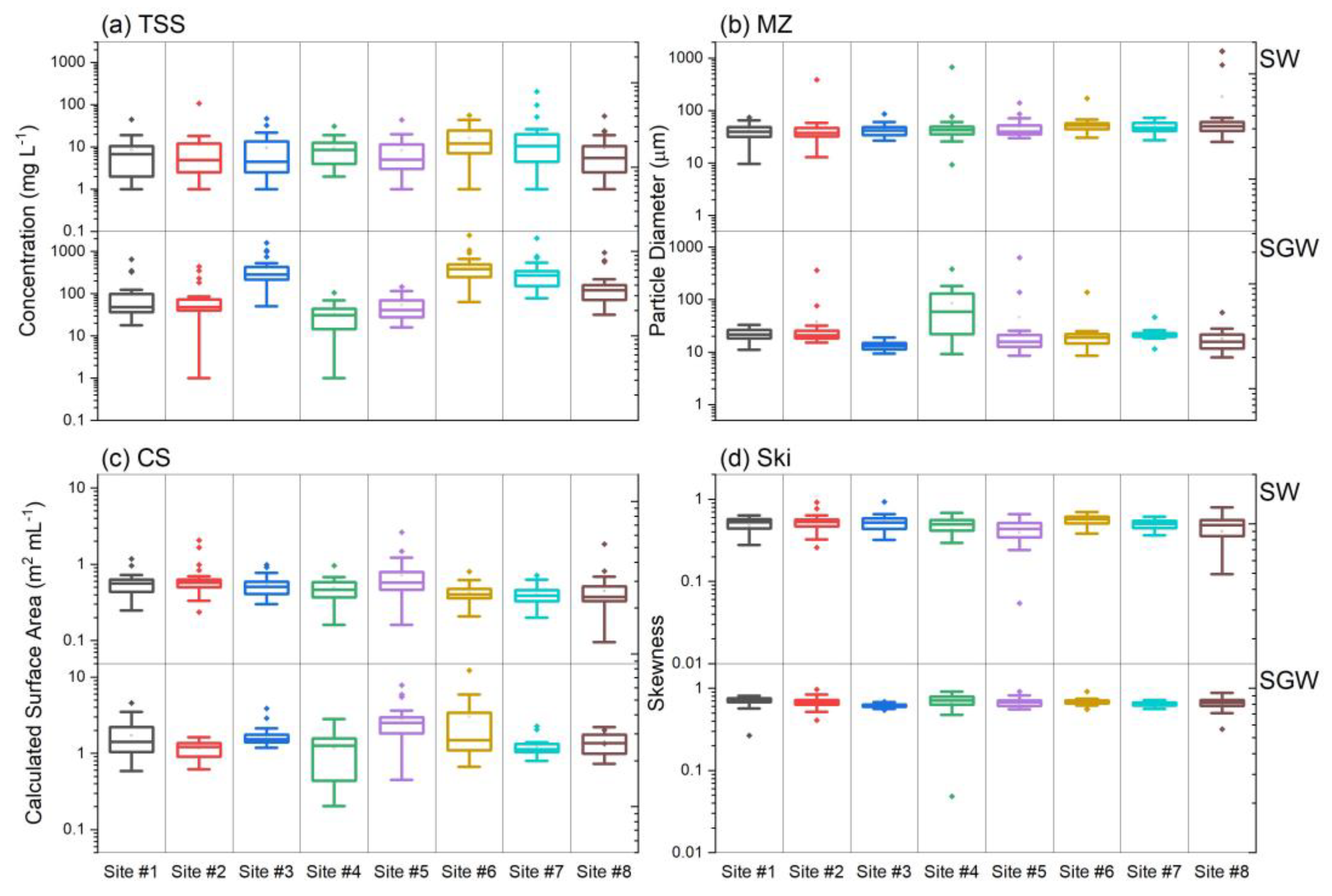
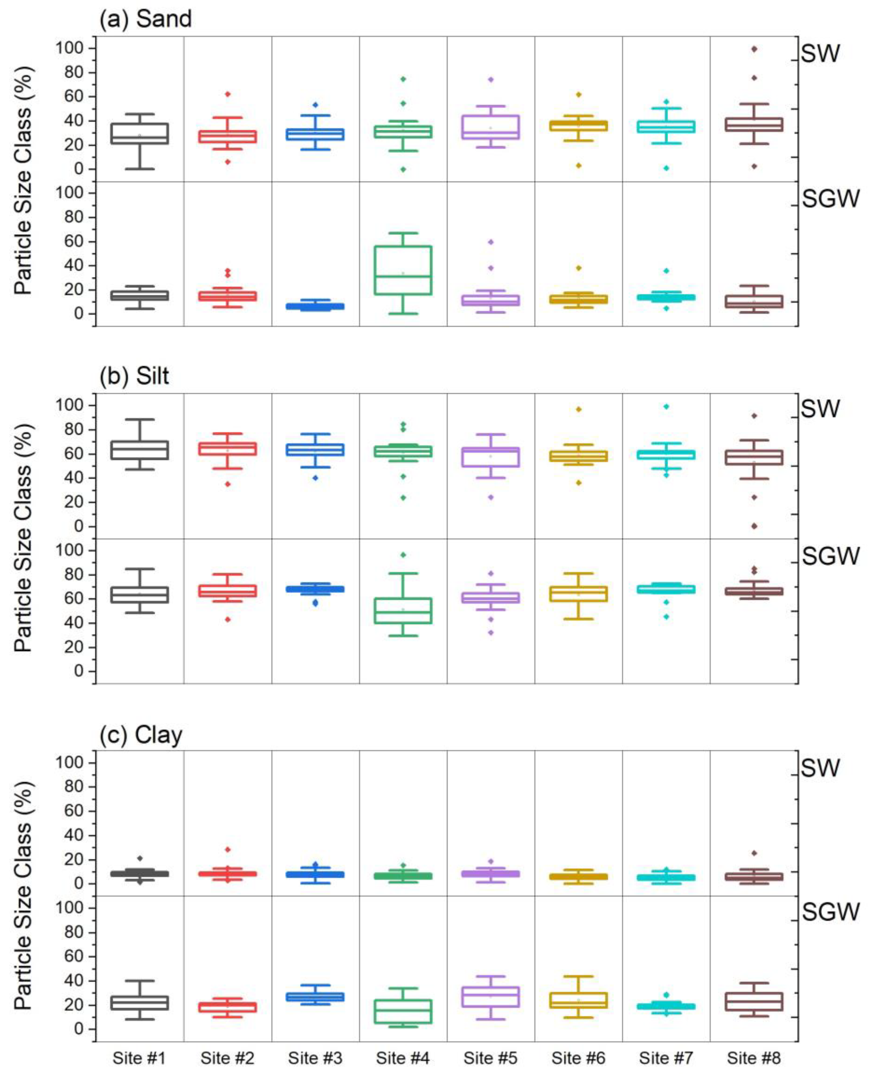
Significant differences (p < 0.05) between at least one pair study of sites were identified for MZ, CS, Ski, sand, silt, and clay in SW samples (Figure 3 and Figure 4; Appendix A, Table A1), while significant differences (p < 0.05) between at least one pair of study sites were identified for TSS, MZ, CS, Ski, sand, silt, and clay in SGW samples (Figure 3 and Figure 4; Appendix A, Table A2). SW suspended sediment characteristics showed variability over the study period, and there was no apparent difference between the upper (i.e., Sites #6, #7, #8) and lower watershed (i.e., Sites #1, #2, #3, #4, #5). For example, SW TSS (mean = 23.50 mg L⁻¹) was highest at Site #7, Site #8 had the largest SW MZ (mean = 184.71 µm) and SW sand percentage (mean = 40.92%), Site #5 exhibited the highest SW CS (mean = 0.72 m² mL⁻¹), SW Ski (mean = 0.53) and largest SW clay percentage (mean = 8.84%) were highest at Site #2, and Site #1 had the largest SW silt percentage (mean = 63.78%).

SGW mean suspended sediment characteristics also showed mixed variability, as Site #6 exhibited the highest SGW TSS (mean = 477.63 mg L⁻¹) and SGW CS (mean = 2.98 m² mL⁻¹). In contrast, Site #4 had the largest SGW MZ (mean = 85.88 µm). SGW sand percentage (mean = 33.56%), Site #1 had the highest SGW Ski (mean = 0.70), and Site #8 had the largest SGW silt percentage (mean = 67.11%). SGW clay percentage (mean = 26.94%) was largest at Site #5. However, there was a more evident difference between the upper (i.e., Sites #6, #7, #8) and lower (i.e., Sites #1, #2, #3, #4, #5) watershed for the SGW suspended sediment characteristic lowest mean values. Site #4 had the lowest SGW TSS (mean = 32.78 mg L⁻¹), lowest SGW CS (mean = 1.17 m² mL⁻¹), smallest SGW silt percentage (mean = 51.30%), and smallest SGW clay percentage (mean = 15.14%) while Site #3 displayed the smallest SGW MZ (mean = 13.20 µm), lowest SGW Ski (mean = 0.61), and smallest SGW sand percentage (mean = 6.35%).

Mean suspended sediment characteristics (TSS, MZ, CS, Ski, sand, silt, and clay; Figure 3) also exhibited inter-site patterns and differences between SW (Table 2) and SGW (Table 3) sources (Figure 4). SGW mean TSS, CS, Ski, and clay percentages were consistently higher than the SW mean values at each study site. Site #6 SGW had the highest mean TSS (477.63 mg/L) and CS (2.98 m² mL⁻¹), Site #1 SGW had the highest mean Ski (0.70), and Site #5 had the highest mean clay percentage (25.94%). At each site, SGW mean TSS was 111–191% higher than SW mean TSS, SGW mean CS was 54–150% higher than SW mean CS, SGW mean ski was 16–47% higher than SW mean ski, and SGW mean clay percentage was 72–123% higher than SW mean clay percentage. These consistent suspended sediment characteristic differences between the sampled water source types in Moore’s Run Watershed demonstrate that SGW had more suspended sediment, comprised of larger proportions of clay particles, relative to the sampled SW. SW mean MZ and sand percentages were 4–164% and 59–130% larger, respectively, than the SGW mean values at most study sites, except for Site #4, which had a mean MZ that was 23% higher than the SW and a mean sand percentage that was 5% larger than the SW. The mean silt percentage was 3–23% larger in the SGW relative to the SW at most study sites, apart from Site #1, which had similar silt percentages (63.78% in the SW and 63.81% in the SGW), and Site #4 where the SW mean silt percentage was 17% larger relative to the SGW. Silt was the most significant proportion of particle size classes at each study site, regardless of the water source type. Clay was the smallest proportion of the SW particle size classes, while sand was the smallest proportion of the SGW particle size classes.

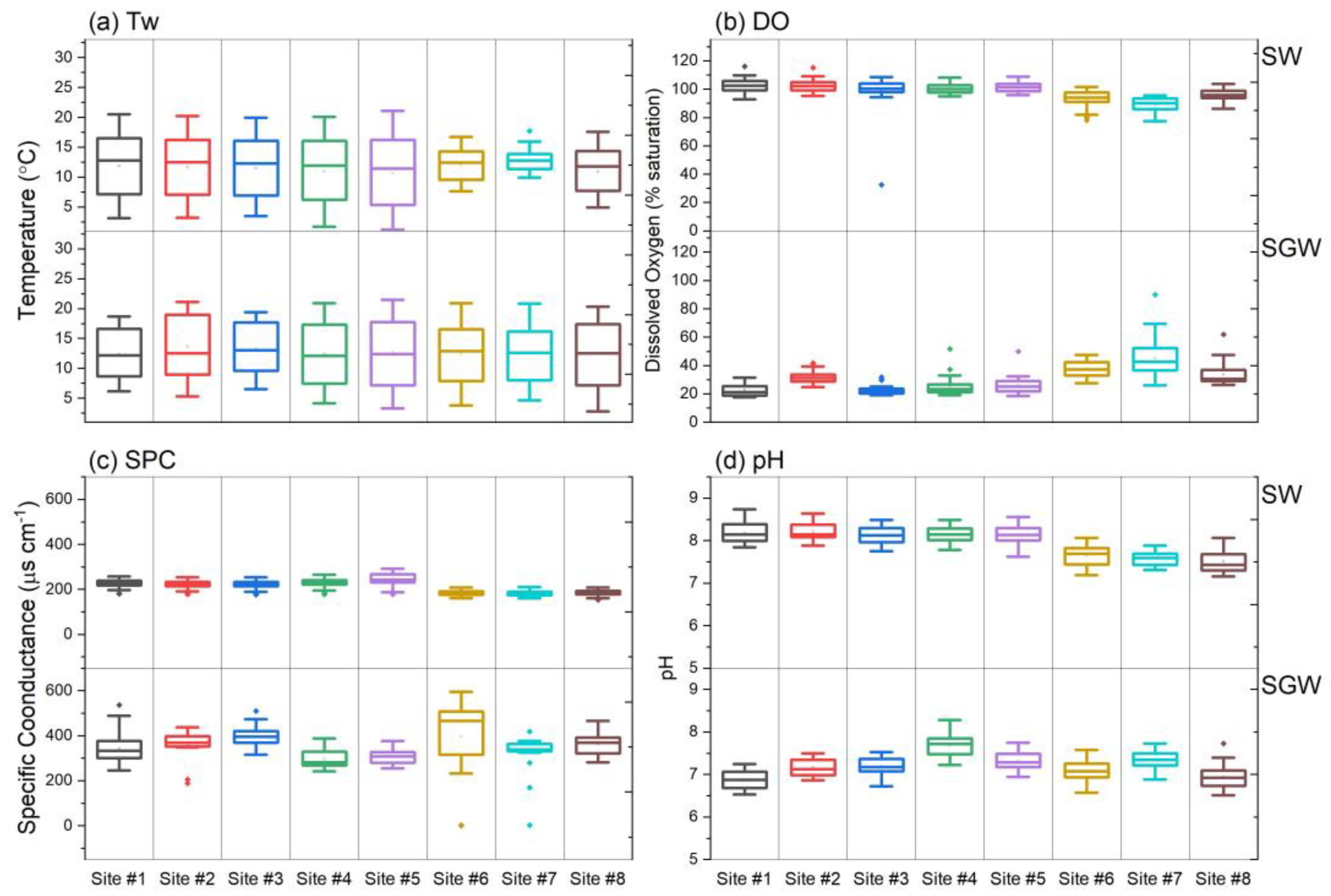
3.4. Physicochemical Variables

Mean physicochemical variables (Tw, DO, SPC, pH; Figure 5) were as expected for both water source types and exhibited patterns with site location. DO and pH values were consistently higher in the SW relative to the SGW (Table 2 and Table 3). Tw and SPC values were typically higher in the SGW relative to the SW (Table 2 and Table 3). Significant differences (p < 0.05) between at least one pair of study sites were identified for Tw, DO, SPC, and pH in SW (Appendix A, Table A1) and SGW samples (Appendix A, Table A2). SW physicochemical variables exhibited variability over the study period, and there was not a consistent difference between the upper (i.e., Sites #6, #7, #8) and lower watershed (i.e., Sites #1, #2, #3, #4, #5). For example, mean SW DO (mean = 102.67% saturation) and pH (8.21) were highest at Site #2, while mean SW Tw and SPC were highest at Site #7 (12.72 °C) and Site #5 (244.87 µs cm⁻¹), respectively. However, SW pH was significantly (p < 0.05) lower at all sites in the upper watershed when compared to the lower watershed (Appendix A, Table A1). SGW physicochemical variables demonstrated more apparent differences between the upper and lower watershed, as the highest and lowest mean physicochemical variables were measured in the lower watershed (i.e., Sites #1, #2, #3, #4, #5), apart from Site #7, which had the highest mean SGW DO (45.33% saturation).

3.5. Principal Component Analysis

The principal components analysis (PCA) included 20 parameters and resulted in five principal components (PCs) with eigenvalues greater than 1 (Appendix A,

Table A3. Results of a principal components analysis comprising 20 variables (i.e., land use percent Agriculture (Ag;%), Forest (For,%), and Developed (Dev,%)], nutrient concentrations (mg L⁻¹), suspended sediment characteristics [total suspended solids; TSS (mg L⁻¹), mean particle size; MZ (µm), calculated surface area; CS (m² mL⁻¹), skewness; Ski, Sand (%), Silt (%), and Clay (%)], and physicochemical variables [water temperature (Tw; °C), dissolved oxygen (DO;% saturation), specific conductance (SPC; µs cm⁻¹), and pH]) used to define five principal components, displaying eigenvalues, percentage of variance, and cumulative variance during the study period (January 2020–December 2021) for eight monitoring sites in Moore’s Run, Watershed, WV, USA. Note: bold numbers indicate Eigen values > 1 (representing importance).

Principal Component	Eigenvalue	Percentage of Variance	Cumulative Variance
1	6.02	30.11%	30.11%
2	3.21	16.07%	46.18%
3	1.96	9.82%	56.00%
4	1.86	9.30%	65.30%
5	1.26	6.29%	71.59%
6	0.94	4.72%	76.31%
7	0.84	4.21%	80.52%
8	0.75	3.76%	84.28%
9	0.69	3.44%	87.71%
10	0.60	3.02%	90.73%
11	0.39	1.93%	92.67%
12	0.31	1.53%	94.20%
13	0.28	1.40%	95.60%
14	0.26	1.30%	96.90%
15	0.23	1.15%	98.05%
16	0.18	0.89%	98.94%
17	0.12	0.62%	99.56%
18	0.09	0.44%	100.00%
19	0.00	0.00%	100.00%
20	0.00	0.00%	100.00%

), which is a standard threshold of importance in PCA [76,94]. Parameters with above average loading influence (> ± 0.22) are italicized in

Table 4. PC Loadings for five principal components (PC) extracted from land use percent [Agriculture (Ag;%), Forest (For,%), and Developed (Dev,%)], nutrient concentrations (mg L⁻¹), suspended sediment characteristics [total suspended solids; TSS (mg L⁻¹), mean particle size; MZ (µm), calculated surface area; CS (m² mL⁻¹), skewness; Ski, Sand (%), Silt (%), and Clay (%)], and physicochemical variables [water temperature (Tw; °C), dissolved oxygen (DO;% saturation), specific conductance (SPC; µs cm⁻¹), and pH] of surface water and shallow groundwater during the study period (January 2020–December 2021) for eight monitoring sites in Moore’s Run, Watershed, WV, USA. Note: italicized entries denote above-average loadings (i.e., PC > 0.22).

Parameter	PC 1	Parameter	PC 2	Parameter	PC 3	Parameter	PC 4	Parameter	PC 5
NH3-N	0.34	Ag	0.49	MZ	0.46	Silt	0.44	Tw	0.65
Clay	0.31	PO43-P	0.21	Sand	0.35	NO2-N	0.3	PO43-P	0.46
TSS	0.3	TP-P	0.2	TN-N	0.28	pH	0.27	NO3-N	0.29
TP-P	0.29	Sand	0.16	TSS	0.26	TN-N	0.27	Ski	0.22
SPC	0.29	DO	0.16	For	0.23	DO	0.24	For	0.11
TN-N	0.27	TSS	0.14	NH3-N	0.23	TSS	0.22	Sand	0.1
CS	0.23	NO2-N	0.13	NO2-N	0.2	NO3-N	0.2	NO2-N	0.06
Ski	0.2	TN-N	0.13	NO3-N	0.19	Tw	0.18	MZ	0.04
NO3-N	0.17	NO3-N	0.1	TP-P	0.17	Dev	0.18	Dev	0.04
Silt	0.13	MZ	0.1	Dev	0.14	For	0.15	NH3-N	−0.01
NO2-N	0.12	Tw	0.04	pH	0.12	TP-P	0.04	SPC	−0.04
Tw	0.09	NH3-N	0.03	SPC	0.04	NH3-N	0.03	Silt	−0.07
Ag	0.07	pH	−0.01	DO	0.01	PO43-P	−0.03	Clay	−0.08
PO43-P	0.01	Silt	−0.05	CS	0.01	SPC	−0.13	Ag	−0.1
For	−0.06	Ski	−0.11	Tw	−0.03	Ag	−0.16	DO	−0.14
Dev	−0.09	CS	−0.16	PO43-P	−0.04	Sand	−0.18	TN-N	−0.14
MZ	−0.15	SPC	−0.17	Clay	−0.05	Clay	−0.21	TSS	−0.16
pH	−0.28	Clay	−0.21	Ski	−0.1	Ski	−0.22	TP-P	−0.17
Sand	−0.29	Dev	−0.46	Ag	−0.23	MZ	−0.28	CS	−0.18
DO	−0.31	For	−0.48	Silt	−0.45	CS	−0.29	pH	−0.25

, and the loadings are included in Figure 6 [95]. The five extracted components explained approximately 72% of the study dataset variance, which included sub-watershed land use, nutrient concentrations, suspended sediment characteristics, and physicochemical variables (Appendix A, Table A3).

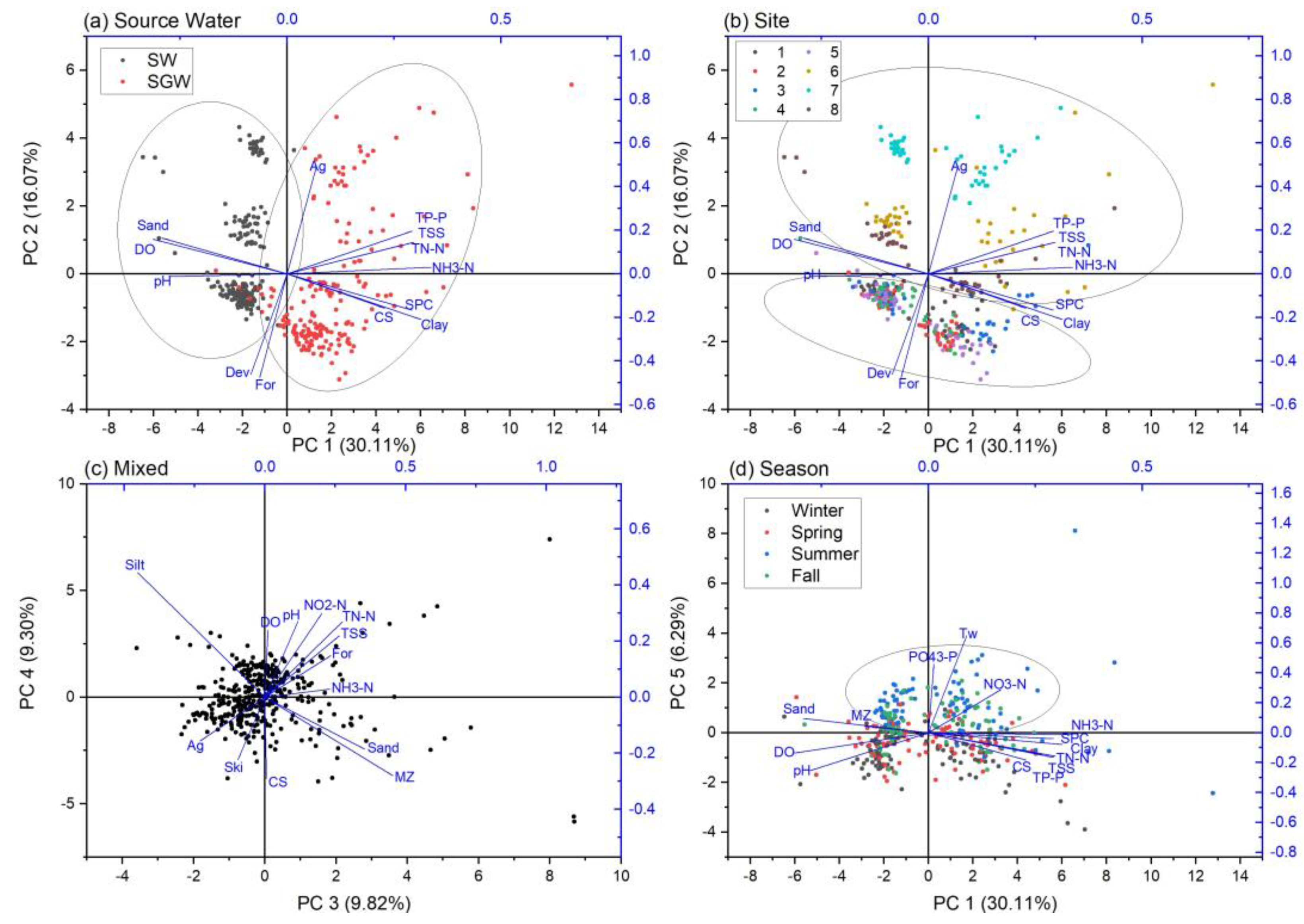
PCA results from the five extracted components were plotted against each other using biplots. The plotted scores were color coded to help visualize any relevant patterns, based on factors known at the time of data collection (i.e., water source type, site location, and sampling season), that might help explain spatiotemporal controls on local water quality. Ovals were added to highlight different groupings. Biplots (Figure 6) exhibited strong data distribution by source water type (i.e., SW or SGW) and watershed location (i.e., study site) along PCs 1 and 2, respectively. PCs 3 and 4 do not demonstrate clear patterns, but PC 5 exhibits a moderate data distribution by season. For example, the point colors in Figure 6a highlight two distinct groups along the x-axis, while the point colors in Figure 6b show eight distinct groupings along the y-axis. The parameters with the above average loadings for PC 1 were NH₃-N, Clay, TSS, TP-P, SPC, TN-N, CS, pH, percentage sand, and DO. In contrast, the above average loadings for PC 2 were limited to land cover percentages (i.e., Agriculture, Forest, and Developed) (Table 4). PC 1 represents water quality differences associated with stream and shallow groundwater environments. PC 2 represents differences in water quality between the upper (i.e., Sites #6, #7, #8) and lower (i.e., Sites #1, #2, #3, #4, #5) watershed, with clear distinctions between the sub-catchment study sites. Ovals shown in Figure 6a denote the separation between SW and SGW samples. Ovals shown in Figure 6b highlight the difference between the upper and lower watershed.

Parameters with above average loadings for PC 3 were MZ, percentage sand, TN-N, TSS, percentage forest cover, NH₃-N, percentage agriculture cover, and silt percentage (Table 4). PC 4 above average loadings were silt percentage, NO₂-N, pH, TN-N, DO, TSS, MZ, and CS (Table 4). Despite eigenvalues greater than 1, PCs 3 and 4 did not show clear patterns by water source type, spatial location, or temporal scale. Thus, PCs 3 and 4 represent mixed factors that may influence water quality outcomes throughout Moore’s Run Watershed (Figure 6c), as demonstrated by the relatively low variance percentages (<10%; Appendix A,

Table A4. Spearman’s correlation results, including land use percent [Agriculture (Ag;%), Forest (For,%), and Developed (Dev,%)], nutrient concentrations (mg L⁻¹), suspended sediment characteristics [total suspended solids; TSS (mg L⁻¹), mean particle size; MZ (µm), calculated surface area; CS (m² mL⁻¹), skewness; Ski, Sand (%), Silt (%), and Clay (%)], and physicochemical variables [water temperature (Tw; °C), dissolved oxygen (DO;% saturation), specific conductance (SPC; µs cm⁻¹), and pH] of surface water and shallow groundwater during the study period (January 2020–December 2021) for eight monitoring sites in Moore’s Run, Watershed, WV, USA. Note: red text indicates significant correlations (p < 0.05). The second portion of the table is a continuance from the preceding.

Variable of Interest	Ag	For	Dev	NO3-N	NO2-N	NH3-N	TN-N	PO43-P	TP-P	TSS
Ag	1
For	−0.85	1
Dev	−0.7	0.7	1
NO3-N	0.05	−0.05	−0.03	1
NO2-N	0.08	−0.1	−0.08	0.25	1
NH3-N	0.02	−0.04	−0.05	0.09	0.75	1
TN-N	0.05	−0.06	−0.06	0.22	0.57	0.58	1
PO43-P	0.33	−0.41	−0.17	−0.04	−0.23	−0.27	−0.22	1
TP-P	0.52	−0.53	−0.45	0.17	0.6	0.63	0.39	0.21	1
TSS	0.19	−0.21	−0.21	0.17	0.78	0.79	0.51	−0.23	0.7	1
MZ	0.01	−0.04	−0.06	−0.14	−0.59	−0.6	−0.38	0.27	−0.47	−0.66
CS	−0.06	0.14	0.12	0.01	0.6	0.66	0.32	−0.34	0.42	0.66
Ski	0.02	−0.04	0.02	−0.02	0.48	0.61	0.19	−0.19	0.4	0.56
Sand	0.02	−0.03	−0.06	−0.1	−0.57	−0.58	−0.39	0.28	−0.44	−0.63
Silt	−0.02	−0.03	0.03	0.19	0.23	0.15	0.28	−0.13	0.12	0.23
Clay	−0.06	0.11	0.09	0.03	0.65	0.68	0.34	−0.35	0.46	0.71
Tw	0.01	−0.03	−0.02	0.31	0.1	0.26	0.09	0.05	0.15	0.08
DO	−0.01	0.01	−0.01	0.06	−0.5	−0.75	−0.29	0.11	−0.54	−0.65
SPC	−0.16	0.16	0.16	0.09	0.58	0.69	0.39	−0.42	0.34	0.66
pH	−0.3	0.3	0.21	−0.02	−0.43	−0.58	−0.23	0.02	−0.6	−0.63
Continued…	MZ	CS	Ski	Sand	Silt	Clay	Tw	DO	SPC	pH
Ag
For
Dev
NO3-N
NO2-N
NH3-N
TN-N
PO43-P
TP-P
TSS
MZ	1
CS	−0.77	1
Ski	−0.33	0.61	1
Sand	0.97	−0.74	−0.33	1
Silt	−0.57	0.17	−0.06	−0.65	1
Clay	−0.81	0.96	0.61	−0.76	0.17	1
Tw	−0.11	−0.01	0.13	−0.11	0.16	0.01	1
DO	0.55	−0.61	−0.61	0.53	−0.12	−0.62	−0.21	1
SPC	−0.64	0.69	0.52	−0.63	0.27	0.7	0.03	−0.62	1
pH	0.52	−0.5	−0.5	0.5	−0.18	−0.53	−0.22	0.75	−0.53	1

).

However, when considering the additional variance explained by PC 5 (6.29%) in the same idealized vector space as PC 1, another pattern emerged that partially explains seasonal controls on water quality at Moore’s Run Watershed. The point colors in Figure 6d represent winter (December, January, and February), spring (March, April, and May), summer (June, July, August), and fall (September, October, and November). There is a clear distinction along the y-axis between water samples collected in the summer, as shown by the oval in Figure 6d, and the remaining seasons (i.e., fall, winter, and spring). Winter and spring water samples appear to be evenly distributed along the negative portion of the y-axis. In contrast, fall samples reflect a range of seasonal conditions due to the distribution along the positive and negative portions of the y-axis. The most substantial loadings for PC 5 were Tw, PO₄³-P, NO₃-N, and pH (Table 4).

PCA results can also show correlations between water quality parameters, physicochemical measurements, and sub-watershed land use percentages [76]. Patterns from the PCs with the largest variance percentages (i.e., PCs 1 and 2) included a significant positive correlation (p < 0.05) between sand percentage and DO; a significant (p < 0.05) positive correlation of percentage forest and developed land cover; a strong and significantly (p < 0.05) negative correlation of percentage agriculture with the other land use percentages; a strong and significant (p < 0.05) association between SPC, CS, and clay percentage; a strong and significant (p < 0.05) negative correlation of pH and NH₃-N; and a significant (p < 0.05) positive association between TSS, TN-N, and TP-P. Support for these conclusions can be found in Appendix A, Table A4, which includes the results of Spearman’s correlation test with the same land use percentages, nutrient concentrations, suspended sediment characteristics, and physicochemical variables assessed for the PCA.

4. Discussion

4.1. Nutrient Concentrations, Suspended Sediment Characteristics, and Physicochemical Variables

Study results showed significant (p < 0.05) differences in nutrient concentrations and suspended sediment characteristics between stream water (SW) and shallow groundwater (SGW) at the eight co-located study sites. Given the proximity of the study sites, along with similar geological, topographical, and climatological conditions, it is reasonable to conclude that water source type (i.e., SW or SGW) and sub-catchment (i.e., study site) location are driving those differences. The results from Site #6 SGW may, in part, reflect the study site piezometer location adjacent to a buried culvert pipe that may have created an artificial hydraulic boundary that influences nutrient and suspended sediment transport to and through the SGW [67]. Notable differences between SW and SGW included higher NO₂-N, NH₃-N, and TP-P concentrations in SGW, lower total suspended solids (TSS) concentrations made up of larger particles in the SW, and higher dissolved oxygen (DO) and pH in the SW.

The observed differences in nutrient concentrations were likely attributable to several factors, including land use (forested and agricultural), agricultural practices (i.e., fertilizer application and livestock grazing), streamflow, shallow groundwater flow, stream-shallow groundwater mixing, and precipitation inputs [96,97,98]. Previous studies have also observed consistent differences between SW and SGW nutrient concentrations [99,100]. For example, Chinnasamy and Hubbart [101] measured NO₃⁻, P, K, and NH₄⁺ concentrations in SW from an Ozark stream and SGW from the riparian hardwood forest. They found that average nutrient concentrations were lower in the SGW relative to the SW, suggesting the importance of riparian vegetation and local geology on nutrient removal processes. Not surprisingly, the SGW nutrient concentrations were higher at Reymann Memorial Farm due to the influence of agricultural land use practices on each sub-catchment [102].

The 111–191% lower TSS concentrations in SW relative to the SGW in Moore’s Run Watershed demonstrate significant differences (p < 0.05) in suspended sediment characteristics between source water types. These differences may be attributed to the permeability of the catchment soil matrix, aquifer material deflocculation, surface water dilution, and land use/land cover [17,103,104]. Gootman and Hubbart [41] noted that the peristaltic pump used for SGW sampling may have influenced the suspended sediment characteristic by creating suction while sampling, thereby affecting the results of the current study. Interestingly, using peristaltic pumps for SGW sampling is common in hydrological studies but may have mobilized additional shallow aquifer sediments [105,106]. Therefore, this complexity shown quantitatively in the current work may also provide the basis for future investigations of GW extraction methods and impacts on measured water quality variables.

Physicochemical results further demonstrated distinct differences between SW and SGW throughout Moore’s Run Watershed. Mean DO concentrations were 65–128% higher in the SW relative to the SGW. Krause et al. [107] observed similar differences in DO concentrations between SW and SGW environments. Mean pH values were 3–17% higher in the SW relative to the SGW. These differences in pH between the two water source types may be due to precipitation and runoff inputs on SW and exposure to minerals in the unconfined alluvial aquifer on SGW [65,108].

One of the most important results of this work is the observed differences in SW and SGW across Moore’s Run Watershed, which is expected but notable as this paired SW/SGW water quality data sets collected at the spatiotemporal scales of this study are unique for the region. When averaged together for the entire study catchment, the SW had 9–148% higher nutrient concentrations, except for PO₄³-P, which was 34% higher in the SW. Suspended sediment characteristics showed that the SW had a 68% larger MZ. In comparison, the SGW had 179% higher TSS, 108% higher CS, and 34% higher Ski, indicating that the SGW had higher suspended sediment concentrations comprising smaller particles relative to the SW. These differences were confirmed by the water source type average particle size distribution results, as the SW had 75% more sand particles. The SGW had 5% and 102% more silt and clay particles, respectively. When averaged by source water type, the physicochemical results demonstrated that the SW DO was 104% higher and the SW pH was 10% higher, while the SGW Tw was 10% higher and the SGW SPC was 49% higher.

The differences by water source type may suggest distinct water quality characteristics for SW and SGW that have different potentials to influence non-point source pollutant loading throughout the study watershed and similar agriculturally influenced catchments [109,110]. These quantitative results support the recommendation that SW and SGW be monitored in situ to quantify relevant water quality outcomes accurately. Results are further supported by the distinct features of Moore’s Run Watershed SW and SGW that are illustrated by the principal components analysis (PCA). The two ovals in the Figure 6a biplot demonstrate distinct differences between SW and SGW when nutrient concentrations, suspended sediment characteristics, physicochemical conditions, and land use are evaluated together.

Site location within the study watershed was also important for water quality outcomes. Additional distinctions between the upper (i.e., Sites #6, #7, #8) and lower watershed (i.e., Sites #1, #2, #3, #4, #5) were evident from the observed nutrient concentrations suspended sediment characteristic, and physicochemical results, which may be attributable to lower forested land cover and higher agricultural land use in the upper watershed (Table 1). SGW nutrient concentrations were consistently higher (47–119%) in the upper watershed relative to the lower watershed. Differences between the upper and lower watershed were inconsistent in the SW, as nutrient concentrations were higher (<1–28%) in the lower watershed for NO₃-N, NO₂-N, and TN-N and lower (1–118%) higher in the upper watershed for NH₃-N, PO₄³-P, and TP-P. Suspended sediment characteristics and physicochemical parameter differences between the upper and lower watershed were more variable for both water source types when comparing the upper and lower watersheds [111,112,113]. TSS was 54% and 85% higher in the upper watershed for both water source types, while SW MZ was 62% higher in the upper watershed, and SGW MZ was 64% higher in the lower watershed. SW CS and Ski 33% and 1% higher in the lower watershed, while SGW CS and Ski were 9% and 1% higher in the upper watershed. SW sand was 20% higher in the upper watershed and 29% for SGW in the lower watershed. Silt and clay were 7% and 34% higher in the lower watershed SW and 6% and <1% higher in the upper watershed SGW. SW Tw was 5% higher in the upper watershed, and SGW Tw was 3% higher in the lower watershed. SW DO, SPC, and pH were 9%, 22%, and 7% higher, respectively, in the lower watershed, while SGW DO and SPC were 41% and 6% higher, respectively, in the upper watershed. SGW pH was 2% higher in the lower watershed. The PCA results support these differences by watershed location (Figure 6). The two ovals in Figure 6b designate study site groupings as a proxy for watershed location and how those differences may influence observed outcomes. The effect of watershed location was associated with land use differences in previous studies [34,114,115]. For example, [116] found differences in NO₃⁻ concentrations between upper and lower watersheds explained by additional denitrification in upland forest areas.

Although most of the Moore’s Run Watershed sub-catchments had similar forested land cover percentages, differences in agricultural land cover percentages between the upper and lower watersheds may be driving these watershed-scale differences (Table 1). For example, Coulter et al. [96] examined non-point pollutant sources in three watersheds and found that agricultural land use significantly increased nutrient concentrations while mixed-land use watersheds had higher TSS fluxes. Thus, agricultural land use practices are understood to influence water quality. In Moore’s Run Watershed, the varying range of agricultural land use in the upper watershed may have resulted in distinct water quality outcomes, as noted in Figure 6b biplot. Conversely, the lower watershed sites were more mixed, with agricultural land use percentages < 10.5% (Table 1). Interestingly, Figure 6b also displays the distinct attributes of Site #7, which is sourced from a known spring in Moore’s Run Watershed (Figure 1).

Seasonal controls were not a primary focus in the current work. However, Figure 6d biplot shows that water samples collected in the summer months (i.e., June, July, and August) were distinct relative to the other months. The PCA results confirm that season variably influences SW and SGW at Moore’s Run Watershed over a year. These findings are supported by previous work, as climatic factors such as air temperature, water temperature, precipitation inputs, and evapotranspiration may vary between seasons and affect water quality [117,118,119,120]. For example, Petersen and Hubbart [121] evaluated water quality results from a mixed land use watershed in the Northeastern United States every quarter and showed that water quality outcomes were variable throughout the year. Thus, the PCA results from the current study reveal some seasonal controls on sub-catchment water quality in Moore’s Run Watershed.

4.2. Principle Components Analysis

Study results show how PCA can be used to characterize water quality data that may inform land and water resource management decisions [76,91,122]. For example, Tripathi and Singal [122] utilized PCA to select parameters for developing a Water Quality Index (WQI) for a river in India. PCA reduced the number of required parameters from 29 to nine, reducing the monitoring time, effort, and cost required to develop the WQI for the Ganga River [122]. The current study’s PCA biplots (Figure 6) demonstrate the importance of water source type, sub-catchment location or spatial variability, and season on water quality outcomes, which could help guide mitigation strategies to reduce nutrient and sediment watershed exports [123].

PCA results suggest strong linkages between TSS, TN-N, and TP-P in SW and SGW, found in other agriculturally influenced watersheds [35,124]. Strong associations between nutrients and suspended sediment in watersheds with relatively low percentages of agriculture and developed land cover suggest that TSS reduction practices can effectively reduce suspended sediments, nitrogen, and phosphorus [54,59,125]. However, further study is needed to explore how observed SW and SGW nutrient concentrations would respond to new TSS management decisions at the watershed scale. Still, the inclusion of SGW water quality results will help constrain pollutant export predictions from small, agro-forested watersheds, which can, in turn, improve large-scale pollutant loading estimates [41].

Additional PCA linkages of note include associations between physicochemical parameters and suspended sediment characteristics. The sand percentage was strongly associated with DO, and the clay percentage was related to calculated surface area (CS) and specific conductivity (SPC), suggesting that suspended sediment particle size is linked to water quality in Moore’s Run Watershed (Figure 6). This linkage implies that in-stream processes that entrain, transport, and store suspended sediment are essential for understanding watershed material transport and water quality outcomes [126]. However, SGW estimates are also needed to constrain non-point source pollutant loading estimates and better predict SW and SGW water quality outcomes [41].

4.3. Study Implications

Implications of the current work extend beyond measuring water quality outcomes in a small, agro-forested watershed. Moore’s Run Watershed is representative of headwater regions in the Chesapeake Bay Watershed (CBW) and similar catchments that support agricultural land use in temperate environments globally. The current work’s experimental watershed approach improved the understanding of how land use and non-point source pollutant loading influence SW and SGW quality [58,127]. Previous studies have shown differences in water quality in SW and SGW from agriculturally influenced catchments [128,129] and the importance of constraining suspended sediment loading regimes to meet regional water quality goals [2,130]. However, studies do not typically include in situ water quality measures of SW and SGW, which adds additional uncertainty to the role of SGW on non-point source pollutant loading [98,113]. The relative differences in nutrient concentrations and suspended sediment characteristics observed in Moore’s Run Watershed SW and SGW are important for non-point source loading predictions [4,124], typically based on surface water measurements [1,131]. Furthermore, if SGW suspended sediment characteristics are ignored, pollutant transport models may underestimate the loading of suspended sediment and particulate nutrients such as phosphorus, which is still increasing in the CBW and similar watersheds globally [51,132].

5. Conclusions

A two-year study was conducted to quantitatively characterize stream water (SW) and shallow groundwater (SGW) nutrient concentration and suspended sediment differences in an agro-forested watershed using a nested-scale, experimental watershed study design. The study watershed was partitioned into eight sub-catchments of varying sizes, each with co-located SW and SGW gauging sites. Monthly grab samples were collected from each site and analyzed in the laboratory for nutrient concentrations with spectrophotometric methods, total suspended solids (TSS) via gravimetric methods, and additional suspended sediment characteristics using laser particle diffraction. Physicochemical parameters were measured in situ at the time of sampling. Data were analyzed with non-parametric methods, a correlation analysis, and a principal components analysis (PCA).

Significant differences (p < 0.05) between study sites were identified for every measured parameter except for SW NO₂-N and SW TSS. Distinct differences between SW and SGW nutrient concentrations suspended sediment characteristics, and physicochemical variables could be explained by a combination of the water source (i.e., stream versus shallow groundwater) and site location within the study watershed (i.e., spatial variability). Nutrient concentrations were higher in the SGW relative to the SW, except for PO₄³-P. SGW samples were characterized by higher TSS concentrations comprising smaller particles, which were confirmed by particle size distribution results. Physicochemical results confirmed that environmental factors, including atmospheric and geologic, influence each water source type. PCA results showed that water source type, spatial variability, and season explained over 52% of the dataset variability. Sub-catchment land use percentages were associated with measured nutrient and suspended sediment concentrations.

These results demonstrate consistent and significant (p < 0.05) differences between SW and SGW throughout the same watershed. Additionally, these results show how water source type, spatial variability, season, and land use practices can influence water quality outcomes in a mixed land use watershed. This critical observation may hold implications for advancing non-point source pollutant loading models that inform policy decisions intended to reduce diffuse pollutants in the Chesapeake Bay Watersheds and similar catchments.

References

- Carpenter, S.R.; Caraco, N.F.; Correll, D.L.; Howarth, R.W.; Sharpley, A.N.; Smith, V.H. Nonpoint Pollution of Surface Waters with Phosphorus and Nitrogen. Ecol. Appl. 1998, 8, 559–568. [Google Scholar] [CrossRef]
- Noe, G.B.; Cashman, M.J.; Skalak, K.; Gellis, A.; Hopkins, K.G.; Moyer, D.; Webber, J.; Benthem, A.; Maloney, K.; Brakebill, J.; et al. Sediment dynamics and implications for management: State of the science from long-term research in the Chesapeake Bay watershed, USA. WIREs Water 2020, 7, e1454. [Google Scholar] [CrossRef]
- Syvitski, J.P.; Vörösmarty, C.J.; Kettner, A.J.; Green, P. Impact of humans on the flux of terrestrial sediment to the global coastal ocean. Science 2005, 308, 376–380. [Google Scholar] [CrossRef] [PubMed]
- Edwards, A.C.; Withers, P.J.A. Transport and delivery of suspended solids, nitrogen and phosphorus from various sources to freshwaters in the UK. J. Hydrol. 2008, 350, 144–153. [Google Scholar] [CrossRef]
- Vilmin, L.; Mogollón, J.M.; Beusen, A.H.W.; Bouwman, A.F. Forms and subannual variability of nitrogen and phosphorus loading to global river networks over the 20th century. Glob. Planet. Chang. 2018, 163, 67–85. [Google Scholar] [CrossRef]
- Beusen, A.H.W.; Bouwman, A.F.; Van Beek, L.P.H.; Mogollón, J.M.; Middelburg, J.J. Global riverine N and P transport to ocean increased during the 20th century despite increased retention along the aquatic continuum. Biogeosciences 2016, 13, 2441–2451. [Google Scholar] [CrossRef] [Green Version]
- Green, P.A.; Vörösmarty, C.J.; Meybeck, M.; Galloway, J.N.; Peterson, B.J.; Boyer, E.W. Pre-industrial and contemporary fluxes of nitrogen through rivers: A global assessment based on typology. Biogeochemistry 2004, 68, 71–105. [Google Scholar] [CrossRef]
- Boyer, E.W.; Howarth, R.W.; Galloway, J.N.; Dentener, F.J.; Green, P.A.; Vörösmarty, C.J. Riverine nitrogen export from the continents to the coasts. Glob. Biogeochem. Cycles 2006, 20, GB1S91. [Google Scholar] [CrossRef] [Green Version]
- Howarth, R.W.; Billen, G.; Swaney, D.; Townsend, A.; Jaworski, N.; Lajtha, K.; Downing, J.A.; Elmgren, R.; Caraco, N.; Jordan, T.; et al. Regional nitrogen budgets and riverine N & P fluxes for the drainages to the North Atlantic Ocean: Natural and human influences. Biogeochemistry 1996, 35, 75–139. [Google Scholar] [CrossRef]
- Vitousek, P.M.; Aber, J.D.; Howarth, R.W.; Likens, G.E.; Matson, P.A.; Schindler, D.W.; Schlesinger, W.H.; Tilman, D.G. Human Alteration of the Global Nitrogen Cycle: Sources and Consequences. Ecol. Appl. 1997, 7, 737–750. [Google Scholar] [CrossRef]
- Peterson, B.J.; Wollheim, W.M.; Mulholland, P.J.; Webster, J.R.; Meyer, J.L.; Tank, J.L.; Martí, E.; Bowden, W.B.; Valett, H.M.; Hershey, A.E.; et al. Control of Nitrogen Export from Watersheds by Headwater Streams. Science 2001, 292, 86–90. [Google Scholar] [CrossRef] [PubMed]
- Ward; Tockner, K. Biodiversity: Towards a unifying theme for river ecology. Freshw. Biol. 2001, 46, 807–819. [Google Scholar] [CrossRef]
- Marzadri, A.; Tonina, D.; Bellin, A.; Tank, J.L. A hydrologic model demonstrates nitrous oxide emissions depend on streambed morphology. Geophys. Res. Lett. 2014, 41, 5484–5491. [Google Scholar] [CrossRef] [Green Version]
- Milliman, J.D.; Meade, R.H. World-Wide Delivery of River Sediment to the Oceans. J. Geol. 1983, 91, 1–21. [Google Scholar] [CrossRef]
- Zeiger, S.J.; Hubbart, J.A. Characterizing Land Use Impacts on Channel Geomorphology and Streambed Sedimentological Characteristics. Water 2019, 11, 1088. [Google Scholar] [CrossRef] [Green Version]
- Zeiger, S.; Hubbart, J. Assessing the Difference between Soil and Water Assessment Tool (SWAT) Simulated Pre-Development and Observed Developed Loading Regimes. Hydrology 2018, 5, 29. [Google Scholar] [CrossRef] [Green Version]
- Borda, T.; Celi, L.; Zavattaro, L.; Sacco, D.; Barberis, E. Effect of agronomic management on risk of suspended solids and phosphorus losses from soil to waters. J. Soils Sediments 2011, 11, 440–451. [Google Scholar] [CrossRef]
- Ferreira, C.S.S.; Walsh, R.P.D.; Kalantari, Z.; Ferreira, A.J.D. Impact of Land-Use Changes on Spatiotemporal Suspended Sediment Dynamics within a Peri-Urban Catchment. Water 2020, 12, 665. [Google Scholar] [CrossRef] [Green Version]
- Beusen, A.H.W.; Dekkers, A.L.M.; Bouwman, A.F.; Ludwig, W.; Harrison, J. Estimation of global river transport of sediments and associated particulate C, N, and P. Glob. Biogeochem. Cycles 2005, 19, GB4S05. [Google Scholar] [CrossRef]
- Chalmers, A.T.; Van Metre, P.C.; Callender, E. The chemical response of particle-associated contaminants in aquatic sediments to urbanization in New England, U.S.A. J. Contam. Hydrol. 2007, 91, 4–25. [Google Scholar] [CrossRef]
- Nasrabadi, T.; Ruegner, H.; Sirdari, Z.Z.; Schwientek, M.; Grathwohl, P. Using total suspended solids (TSS) and turbidity as proxies for evaluation of metal transport in river water. Appl. Geochem. 2016, 68, 1–9. [Google Scholar] [CrossRef]
- Correll, D.L. Phosphorus: A rate limiting nutrient in surface waters. Poult. Sci. 1999, 78, 674–682. [Google Scholar] [CrossRef]
- Gruszowski, K.E.; Foster, I.D.L.; Lees, J.A.; Charlesworth, S.M. Sediment sources and transport pathways in a rural catchment, Herefordshire, UK. Hydrol. Process. 2003, 17, 2665. [Google Scholar] [CrossRef]
- Zeiger, S.J.; Hubbart, J.A. Nested-Scale Nutrient Flux in a Mixed-Land-Use Urbanizing Watershed. Hydrol. Process. 2016, 30, 1475–1490. [Google Scholar] [CrossRef]
- Schilling, K.E.; Isenhart, T.M.; Palmer, J.A.; Wolter, C.F.; Spooner, J. Impacts of Land-Cover Change on Suspended Sediment Transport in Two Agricultural Watersheds1. JAWRA J. Am. Water Resour. Assoc. 2011, 47, 672–686. [Google Scholar] [CrossRef]
- Hughes, A.O.; Quinn, J.M.; McKergow, L.A. Land use influences on suspended sediment yields and event sediment dynamics within two headwater catchments, Waikato, New Zealand. N. Z. J. Mar. Freshw. Res. 2012, 46, 315–333. [Google Scholar] [CrossRef] [Green Version]
- Powers, S.M.; Tank, J.L.; Robertson, D.M. Control of nitrogen and phosphorus transport by reservoirs in agricultural landscapes. Biogeochemistry 2015, 124, 417–439. [Google Scholar] [CrossRef]
- Zeiger, S.J.; Hubbart, J.A. Quantifying flow interval–pollutant loading relationships in a rapidly urbanizing mixed-land-use watershed of the Central USA. Environ. Earth Sci. 2017, 76, 484. [Google Scholar] [CrossRef]
- Bajželj, B.; Richards, K.S.; Allwood, J.M.; Smith, P.; Dennis, J.S.; Curmi, E.; Gilligan, C.A. Importance of food-demand management for climate mitigation. Nat. Clim. Chang. 2014, 4, 924–929. [Google Scholar] [CrossRef] [Green Version]
- Van Dijk, M.; Morley, T.; Rau, M.L.; Saghai, Y. A meta-analysis of projected global food demand and population at risk of hunger for the period 2010–2050. Nat. Food 2021, 2, 494–501. [Google Scholar] [CrossRef]
- Tilman, D.; Balzer, C.; Hill, J.; Befort, B.L. Global food demand and the sustainable intensification of agriculture. Proc. Natl. Acad. Sci. USA 2011, 108, 20260–20264. [Google Scholar] [CrossRef] [PubMed] [Green Version]
- Ray, D.K.; Mueller, N.D.; West, P.C.; Foley, J.A. Yield Trends Are Insufficient to Double Global Crop Production by 2050. PLoS ONE 2013, 8, e66428. [Google Scholar] [CrossRef] [PubMed] [Green Version]
- Kopittke, P.M.; Menzies, N.W.; Wang, P.; McKenna, B.A.; Lombi, E. Soil and the intensification of agriculture for global food security. Environ. Int. 2019, 132, 105078. [Google Scholar] [CrossRef] [PubMed]
- Kellner, E.; Hubbart, J.A. Confounded by forgotten legacies: Effectively managing watersheds in the contemporary age of unknown unknowns. Hydrol. Process. 2017, 31, 2802–2808. [Google Scholar] [CrossRef]
- Corriveau, J.; van Bochove, E.; Cluis, D. Sources of nitrite in streams of an intensively cropped watershed. Water Environ. Res. 2010, 82, 622–632. [Google Scholar] [CrossRef]
- Miller, C.V.; Denis, J.M.; Ator, S.W.; Brakebill, J.W. Nutrients in Streams During Baseflow in Selected Environmental Settings of the Potomac River Basin. JAWRA J. Am. Water Resour. Assoc. 1998, 33, 1155. [Google Scholar] [CrossRef]
- Boesch, D.F.; Brinsfield, R.B.; Magnien, R.E. Chesapeake Bay Eutrophication: Scientific Understanding, Ecosystem Restoration, and Challenges for Agriculture. J. Environ. Qual. 2001, 30, 303–320. [Google Scholar] [CrossRef] [Green Version]
- Diego-Feliu, M.; Rodellas, V.; Alorda-Kleinglass, A.; Saaltink, M.; Folch, A.; Garcia-Orellana, J. Extreme precipitation events induce high fluxes of groundwater and associated nutrients to coastal ocean. Hydrol. Earth Syst. Sci. 2022, 26, 4619–4635. [Google Scholar] [CrossRef]
- Reynolds, W. Saturated and field-unsaturated water flow parameters: Laboratory methods. Phys. Methods 2002, 4, 802–817. Available online: https://acsess.onlinelibrary.wiley.com/doi/abs/10.2136/sssabookser5.4.c31 (accessed on 20 September 2022).
- Foster, I.D.L.; Chapman, A.S.; Hodgkinson, R.M.; Jones, A.R.; Lees, J.A.; Turner, S.E.; Scott, M. Changing suspended sediment and particulate phosphorus loads and pathways in underdrained lowland agricultural catchments; Herefordshire and Worcestershire, U.K. Hydrobiologia 2003, 494, 119–126. [Google Scholar] [CrossRef]
- Gootman, K.S.; Hubbart, J.A. A Comparison of Stream Water and Shallow Groundwater Suspended Sediment Concentrations in a West Virginia Mixed-Use, Agro-Forested Watershed. Land 2022, 11, 506. [Google Scholar] [CrossRef]
- Charizopoulos, N.; Zagana, E.; Psilovikos, A. Assessment of natural and anthropogenic impacts in groundwater, utilizing multivariate statistical analysis and inverse distance weighted interpolation modeling: The case of a Scopia basin (Central Greece). Environ. Earth Sci. 2018, 77, 380. [Google Scholar] [CrossRef]
- Jantz, P.; Goetz, S.; Jantz, C. Urbanization and the Loss of Resource Lands in the Chesapeake Bay Watershed. Environ. Manag. 2005, 36, 808–825. [Google Scholar] [CrossRef] [PubMed]
- Kemp, W.M.; Boynton, W.R.; Adolf, J.E.; Boesch, D.F.; Boicourt, W.C.; Brush, G.; Cornwell, J.C.; Fisher, T.R.; Glibert, P.M.; Hagy, J.D. Eutrophication of Chesapeake Bay: Historical trends and ecological interactions. Mar. Ecol. Prog. Ser. 2005, 303, 1–29. [Google Scholar] [CrossRef] [Green Version]
- Barlow, R.A.; Brakebill, J.W.; Bratton, J.F.; Blazer, V.S.; Bohlke, J.K.; Bricker, O.P.; Colman, S.M.; Cronin, T.M.; Hupp, C.R.; Keough, J.R.; et al. The U.S. Geological Survey and the Chesapeake Bay—The Role of Science in Environmental Restoration; Circular 1220; USGS: Reston, VA, USA, 2002. [Google Scholar]
- Brakebill, J.; Ator, S.; Sekellick, A. Input and predictions from a suspended-sediment SPARROW model CBSS_V2 in the Chesapeake Bay Watershed; US Geological Survey Data Release; USGS: Reston, VA, USA, 2019. [Google Scholar]
- Boesch, D.F.; Greer, J. Chesapeake Futures: Choices for the 21st Century; Chesapeake Research Consortium: Edgewater, MD, USA, 2003. [Google Scholar]
- USEPA. Chesapeake Bay Total Maximum Daily Load for Nitrogen, Phosphorus and Sediment; U.S. Environmental Protection Agency: Washington, DC, USA, 2010.
- Shenk, G.W.; Linker, L.C. Development and Application of the 2010 Chesapeake Bay Watershed Total Maximum Daily Load Model. JAWRA J. Am. Water Resour. Assoc. 2013, 49, 1042–1056. [Google Scholar] [CrossRef]
- Zhang, Q.; Brady, D.C.; Boynton, W.R.; Ball, W.P. Long-Term Trends of Nutrients and Sediment from the Nontidal Chesapeake Watershed: An Assessment of Progress by River and Season. JAWRA J. Am. Water Resour. Assoc. 2015, 51, 1534–1555. [Google Scholar] [CrossRef]
- Langland, M.; Blomquist, J.; Moyer, D.; Hyer, K. Nutrient and Suspended-Sediment Trends, Loads, and Yields and Development of an Indicator of Streamwater Quality at Nontidal Sites in the Chesapeake Bay Watershed, 1985–2010; US Geological Survey Scientific Investigations Report 2012-5093; USGS: Reston, VA, USA, 2012; 26p. [Google Scholar]
- Moyer, D.; Blomquist, J. Summary of Nitrogen, Phosphorus, and Suspended-Sediment Loads and Trends Measured at the Chesapeake Bay Nontidal Network Stations for Water Years 2009–2018. United States Geological Survey Report. 2018. Available online: https://d18lev1ok5leia.cloudfront.net/chesapeakebay/documents/ii.a._ntn_load_and_trend_summary_2018.pdf (accessed on 20 September 2022).
- Zhang, Q. Synthesis of nutrient and sediment export patterns in the Chesapeake Bay watershed: Complex and non-stationary concentration-discharge relationships. Sci. Total Environ. 2018, 618, 1268–1283. [Google Scholar] [CrossRef]
- Williams, M.R.; Bhatt, G.; Filoso, S.; Yactayo, G. Stream restoration performance and its contribution to the Chesapeake Bay TMDL: Challenges posed by climate change in urban areas. Estuaries Coasts 2017, 40, 1227–1246. [Google Scholar] [CrossRef]
- Renwick, W.H.; Andereck, Z.D. Reservoir sedimentation trends in Ohio, USA: Sediment delivery and response to land-use change. IAHS Publ. 2006, 306, 341. [Google Scholar]
- Zeiger, S.J.; Hubbart, J.A. A SWAT model validation of nested-scale contemporaneous stream flow, suspended sediment and nutrients from a multiple-land-use watershed of the central USA. Sci Total Environ. 2016, 572, 232–243. [Google Scholar] [CrossRef]
- Zhang, Q.; Ball, W.P.; Moyer, D.L. Decadal-scale export of nitrogen, phosphorus, and sediment from the Susquehanna River basin, USA: Analysis and synthesis of temporal and spatial patterns. Sci. Total Environ. 2016, 563–564, 1016–1029. [Google Scholar] [CrossRef] [PubMed] [Green Version]
- Hubbart, J.A.; Kellner, E.; Zeiger, S.J. A Case-Study Application of the Experimental Watershed Study Design to Advance Adaptive Management of Contemporary Watersheds. Water 2019, 11, 2355. [Google Scholar] [CrossRef]
- Bechmann, M.; Stålnacke, P. Effect of policy-induced measures on suspended sediments and total phosphorus concentrations from three Norwegian agricultural catchments. Sci. Total Environ. 2005, 344, 129–142. [Google Scholar] [CrossRef] [PubMed]
- Bainbridge, Z.T.; Brodie, J.E.; Faithful, J.W.; Sydes, D.A.; Lewis, S.E. Identifying the land-based sources of suspended sediments, nutrients and pesticides discharged to the Great Barrier Reef from the Tully-Murray Basin, Queensland, Australia. Mar. Freshw. Res. 2009, 60, 1081. [Google Scholar] [CrossRef]
- Rousseau, A.N.; Savary, S.; Hallema, D.W.; Gumiere, S.J.; Foulon, É. Modeling the effects of agricultural BMPs on sediments, nutrients, and water quality of the Beaurivage River watershed (Quebec, Canada). Can. Water Resour. J. 2013, 38, 99–120. [Google Scholar] [CrossRef]
- NRAC. West Virginia Land Use Land Cover (NAIP 2016); West Virginia GIS Technical Center: Morgantown, WV, USA, 2020. Available online: http://www.mapwv.gov/ (accessed on 20 September 2022).
- Knight, H.G. Reymann Memorial Farms; West Virginia Agricultural and Forestry Experiment Station: Morgantown, WV, USA, 1925; Volume 194, Available online: https://researchrepository.wvu.edu/wv_agricultural_and_forestry_experiment_station_bulletins/194/ (accessed on 20 September 2022).
- WVU. Reymann Memorial Farms West Virginia University. Wardensville, West Virginia, USA. Available online: https://www.davis.wvu.edu/about-davis-college/farms-and-forests/reymann-memorial-farm (accessed on 20 September 2022).
- Nicholson, S.W.; Dicken, C.L.; Horton, J.D.; Labay, K.A.; Foose, M.P.; Mueller, J.A.L. Preliminary Integrated Geologic Map Databases for the United States: Kentucky, Ohio, Tennessee, and West Virginia; Open-File Report 2005-1324; USGS: Reston, VA, USA, 2005. [Google Scholar]
- NRCS. Web Site for Official Soil Series Descriptions and Series Classification. 2020. Available online: https://www.nrcs.usda.gov/resources/data-and-reports/official-soil-series-descriptions-osd (accessed on 20 September 2022).
- Gootman, K.; Kellner, E.; Hubbart, J. A Comparison and Validation of Saturated Hydraulic Conductivity Models. Water 2020, 12, 2040. [Google Scholar] [CrossRef]
- NOAA. Climate Data Online Search. 2020. Available online: https://www.ncdc.noaa.gov/cdo-web/search (accessed on 20 September 2022).
- Zeiger, S.J.; Hubbart, J.A. Quantifying relationships between urban land use and flow frequency of small Missouri streams. Sci. Total Environ. 2019, 659, 1008–1015. [Google Scholar] [CrossRef]
- Hubbart, J.A. Improving Best Management Practice Decisions in Mixed Land Use and/or Municipal Watersheds: Should Approaches Be Standardized? Land 2021, 10, 1402. [Google Scholar] [CrossRef]
- Hubbart, J.A.; Link, T.E.; Gravelle, J.A.; Elliot, W.J. Timber harvest impacts on water yield in the continental/maritime hydroclimatic region of the United States. For. Sci. 2007, 53, 169–180. [Google Scholar]
- Karwan, D.L.; Gravelle, J.A.; Hubbart, J.A. Effects of timber harvest on suspended sediment loads in Mica Creek, Idaho. For. Sci. 2007, 53, 181–188. [Google Scholar]
- Guzman, J.A.; Moriasi, D.N.; Gowda, P.H.; Steiner, J.L.; Starks, P.J.; Arnold, J.G.; Srinivasan, R. A model integration framework for linking SWAT and MODFLOW. Environ. Model. Softw. 2015, 73, 103–116. [Google Scholar] [CrossRef]
- Zeiger, S.; Hubbart, J. Urban Stormwater Temperature Surges: A Central US Watershed Study. Hydrology 2015, 2, 193–209. [Google Scholar] [CrossRef]
- Hubbart, J.; Kellner, E.; Hooper, L.; Lupo, A.; Market, P.; Guinan, P.; Stephan, K.; Fox, N.; Svoma, B. Localized Climate and Surface Energy Flux Alterations across an Urban Gradient in the Central U.S. Energies 2014, 7, 1770–1791. [Google Scholar] [CrossRef] [Green Version]
- Kellner, E.; Hubbart, J.; Stephan, K.; Morrissey, E.; Freedman, Z.; Kutta, E.; Kelly, C. Characterization of sub-watershed-scale stream chemistry regimes in an Appalachian mixed-land-use watershed. Environ. Monit. Assess. 2018, 190, 586. [Google Scholar] [CrossRef]
- Kellner, E.; Hubbart, J.A. Spatiotemporal variability of suspended sediment particle size in a mixed-land-use watershed. Sci. Total Environ. 2018, 615, 1164–1175. [Google Scholar] [CrossRef] [PubMed]
- Hubbart, J.A.; Kellner, E.; Freeman, G. A case study considering the comparability of mass and volumetric suspended sediment data. Environ. Earth Sci. 2014, 71, 4051–4060. [Google Scholar] [CrossRef]
- APHA. 2540 Solids. In Standard Methods For the Examination of Water and Wastewater; American Public Health Association: Washington, DC, USA, 1999. Available online: https://www.standardmethods.org/doi/10.2105/SMWW.2882.030 (accessed on 20 September 2022).
- Plantz, P.E. Pigment Particle Size Using Microtrac Laser Technology; SL-AN-30 Revision A. 2009. Available online: http://www.microtrac.com (accessed on 10 February 2020).
- Plantz, P.E. Blue Laser Technology Applied to the Microtrac Unified Scatter Technique for Full-Range Particle Size Measurement. Application Note; Microtrac, Inc.: Montgomeryville, PA, USA, 2007; 8p. [Google Scholar]
- Agrawal, Y.C.; Whitmire, A.; Mikkelsen, O.A.; Pottsmith, H.C. Light scattering by random shaped particles and consequences on measuring suspended sediments by laser diffraction. J. Geophys. Res. 2008, 113, C04023. [Google Scholar] [CrossRef] [Green Version]
- Kellner, E.; Hubbart, J. Advancing Understanding of the Surface Water Quality Regime of Contemporary Mixed-Land-Use Watersheds: An Application of the Experimental Watershed Method. Hydrology 2017, 4, 31. [Google Scholar] [CrossRef] [Green Version]
- Helsel, D.R.; Hirsch, R.M.; Ryberg, K.R.; Archfield, S.A.; Gilroy, E.J. Statistical Methods in Water Resources; 4-A3; USGS: Reston, VA, USA, 2020; p. 484. [Google Scholar]
- Yazici, B.; Yolacan, S. A comparison of various tests of normality. J. Stat. Comput. Simul. 2007, 77, 175–183. [Google Scholar] [CrossRef]
- Davis, J.C. Statistics and Data Analysis in Geology; Wiley & Sons: New York, NY, USA, 2002; Available online: https://www.kgs.ku.edu/Mathgeo/Books/Stat/ClarifyEq4-81.pdf (accessed on 20 September 2022).
- Friedman, M. The use of ranks to avoid the assumption of normality implicit in the analysis of variance. J. Am. Stat. Assoc. 1937, 32, 675–701. [Google Scholar] [CrossRef]
- Hauke, J.; Kossowski, T. Comparison of Values of Pearson’s and Spearman’s Correlation Coefficients on the Same Sets of Data. Quaest. Geogr. 2011, 30, 87–93. [Google Scholar] [CrossRef] [Green Version]
- Lehr, C.; Pöschke, F.; Lewandowski, J.; Lischeid, G. A novel method to evaluate the effect of a stream restoration on the spatial pattern of hydraulic connection of stream and groundwater. J. Hydrol. 2015, 527, 394–401. [Google Scholar] [CrossRef] [Green Version]
- Jolliffe, I.T.; Cadima, J. Principal component analysis: A review and recent developments. Philos. Trans. R. Soc. A Math. Phys. Eng. Sci. 2016, 374, 20150202. [Google Scholar] [CrossRef] [Green Version]
- Petersen, F.; Hubbart, J.A.; Kellner, E.; Kutta, E. Land-use-mediated Escherichia coli concentrations in a contemporary Appalachian watershed. Environ. Earth Sci. 2018, 77. [Google Scholar] [CrossRef]
- Kutta, E.; Hubbart, J. Changing Climatic Averages and Variance: Implications for Mesophication at the Eastern Edge of North America’s Eastern Deciduous Forest. Forests 2018, 9, 605. [Google Scholar] [CrossRef] [Green Version]
- Kutta, E.; Hubbart, J. Climatic Trends of West Virginia: A Representative Appalachian Microcosm. Water 2019, 11, 1117. [Google Scholar] [CrossRef] [Green Version]
- Linting, M.; Meulman, J.J.; Groenen, P.J.; van der Koojj, A.J. Nonlinear principal components analysis: Introduction and application. Psychol Methods 2007, 12, 336–358. [Google Scholar] [CrossRef] [Green Version]
- Bro, R.; Smilde, A.K. Principal component analysis. Anal. Methods 2014, 6, 2812–2831. [Google Scholar] [CrossRef] [Green Version]
- Coulter, C.B.; Kolka, R.K.; Thompson, J.A. Water Quality in Agricultural, Urban, and Mixed Land Use Watersheds1. JAWRA J. Am. Water Resour. Assoc. 2004, 40, 1593–1601. [Google Scholar] [CrossRef]
- Huizenga, A.; Bailey, R.T.; Gates, T.K. Stream-aquifer and in-stream processes affecting nitrogen along a major river and contributing tributary. J. Contam. Hydrol. 2017, 199, 24–35. [Google Scholar] [CrossRef] [Green Version]
- Murphy, J.C. Changing suspended sediment in United States rivers and streams: Linking sediment trends to changes in land use/cover, hydrology and climate. Hydrol. Earth Syst. Sci. 2020, 24, 991–1010. [Google Scholar] [CrossRef] [Green Version]
- Wieben, C.M.; Baker, R.J.; Nicholson, R.S. Nutrient Concentrations in Surface Water and Groundwater, and Nitrate Source Identification Using Stable Isotope Analysis, in the Barnegat Bay-Little Egg Harbor Watershed, New Jersey, 2010–2011; Scientific Investigations Report 2012-5287; USGS: Reston, VA, USA, 2013; pp. 1–44. [Google Scholar]
- Yu, L.; Rozemeijer, J.; Van Breukelen, B.M.; Ouboter, M.; Van Der Vlugt, C.; Broers, H.P. Groundwater impacts on surface water quality and nutrient loads in lowland polder catchments: Monitoring the greater Amsterdam area. Hydrol. Earth Syst. Sci. 2018, 22, 487–508. [Google Scholar] [CrossRef] [Green Version]
- Chinnasamy, P.; Hubbart, J.A. Stream and shallow groundwater nutrient concentrations in an Ozark forested riparian zone of the central USA. Environ. Earth Sci. 2015, 73, 6577–6590. [Google Scholar] [CrossRef]
- Schröder, J.J.; Scholefield, D.; Cabral, F.; Hofman, G. The effects of nutrient losses from agriculture on ground and surface water quality: The position of science in developing indicators for regulation. Environ. Sci. Policy 2004, 7, 15–23. [Google Scholar] [CrossRef]
- Goldenberg, L.C.; Mandel, S.; Magaritz, M. Fluctuating, non-homogeneous changes of hydraulic conductivity in porous media. Q. J. Eng. Geol. Hydrogeol. 1986, 19, 183–190. [Google Scholar] [CrossRef]
- Florsheim, J.L.; Pellerin, B.A.; Oh, N.H.; Ohara, N.; Bachand, P.A.M.; Bachand, S.M.; Bergamaschi, B.A.; Hernes, P.J.; Kavvas, M.L. From deposition to erosion: Spatial and temporal variability of sediment sources, storage, and transport in a small agricultural watershed. Geomorphology 2011, 132, 272–286. [Google Scholar] [CrossRef]
- Frostick, L.E.; Lucas, P.M.; Reid, I. The infiltration of fine matrices into coarse-grained alluvial sediments and its implications for stratigraphical interpretation. J. Geol. Soc. 1984, 141, 955–965. [Google Scholar] [CrossRef]
- Duff, J.H.; Murphy, F.; Fuller, C.C.; Triska, F.J.; Harvey, J.W.; Jackman, A.P. A mini drivepoint sampler for measuring pore water solute concentrations in the hyporheic zone of sand-bottom streams. Limnol. Oceanogr. 1998, 43, 1378–1383. [Google Scholar] [CrossRef]
- Krause, S.; Heathwaite, L.; Binley, A.; Keenan, P. Nitrate concentration changes at the groundwater-surface water interface of a small Cumbrian river. Hydrol. Process. 2009, 23, 2195. [Google Scholar] [CrossRef]
- Griffioen, J.; Vermooten, S.; Janssen, G. Geochemical and palaeohydrological controls on the composition of shallow groundwater in the Netherlands. Appl. Geochem. 2013, 39, 129–149. [Google Scholar] [CrossRef]
- Cho, J.; Mostaghimi, S.; Kang, M.S. Development and application of a modeling approach for surface water and groundwater interaction. Agric. Water Manag. 2010, 97, 123–130. [Google Scholar] [CrossRef]
- Wainwright, J.; Turnbull, L.; Ibrahim, T.G.; Lexartza-Artza, I.; Thornton, S.F.; Brazier, R.E. Linking environmental regimes, space and time: Interpretations of structural and functional connectivity. Geomorphology 2011, 126, 387–404. [Google Scholar] [CrossRef]
- Martin, J.-M.; Meybeck, M. Elemental mass-balance of material carried by major world rivers. Mar. Chem. 1979, 7, 173–206. [Google Scholar] [CrossRef]
- Meybeck, M. Global analysis of river systems: From Earth system controls to Anthropocene syndromes. Philos. Trans. R. Soc. Lond. B Biol. Sci. 2003, 358, 1935–1955. [Google Scholar] [CrossRef] [PubMed]
- Walling, D.E.; Owens, P.N.; Carter, J.; Leeks, G.J.L.; Lewis, S.; Meharg, A.A.; Wright, J. Storage of sediment-associated nutrients and contaminants in river channel and floodplain systems. Appl. Geochem. 2003, 18, 195–220. [Google Scholar] [CrossRef]
- Dukes, M.D.; Evans, R.O. Impact of Agriculture on Water Quality in the North Carolina Middle Coastal Plain. J. Irrig. Drain. Eng. 2006, 132, 250–262. [Google Scholar] [CrossRef]
- Jones, C.N.; Scott, D.T.; Guth, C.; Hester, E.T.; Hession, W.C. Influence of Sampling Frequency on Estimation of Annual Total Phosphorus and Total Suspended Solids Loads1. JAWRA J. Am. Water Resour. Assoc. 2012, 48, 1258. [Google Scholar] [CrossRef]
- Shinozuka, K.I.; Chiwa, M.; Tayasu, I.; Yoshimizu, C.; Otsuki, K.; Kume, A. Differences in Stream Water Nitrate Concentrations between a Nitrogen-Saturated Upland Forest and a Downstream Mixed Land Use River Basin. Hydrology 2017, 4, 43. [Google Scholar] [CrossRef] [Green Version]
- Griffiths, N.A.; Tank, J.L.; Royer, T.V.; Roley, S.S.; Rosi-Marshall, E.J.; Whiles, M.R.; Beaulieu, J.J.; Johnson, L.T. Agricultural land use alters the seasonality and magnitude of stream metabolism. Limnol. Oceanogr. 2013, 58, 1513–1529. [Google Scholar] [CrossRef]
- Zhang, Q.; Brady, D.C.; Ball, W.P. Long-term seasonal trends of nitrogen, phosphorus, and suspended sediment load from the non-tidal Susquehanna River Basin to Chesapeake Bay. Sci. Total Environ. 2013, 452–453, 208–221. [Google Scholar] [CrossRef]
- Jones, C.N.; Scott, D.T.; Guth, C.; Hester, E.T.; Hession, W.C. Seasonal Variation in Floodplain Biogeochemical Processing in a Restored Headwater Stream. Environ. Sci. Technol. 2015, 49, 13190–13198. [Google Scholar] [CrossRef] [PubMed]
- Zhou, R.; Pan, Z.; Jin, J.; Li, C.; Ning, S. Forewarning Model of Regional Water Resources Carrying Capacity Based on Combination Weights and Entropy Principles. Entropy 2017, 19, 574. [Google Scholar] [CrossRef] [Green Version]
- Petersen, F.; Hubbart, J.A. Advancing Understanding of Land Use and Physicochemical Impacts on Fecal Contamination in Mixed-Land-Use Watersheds. Water 2020, 12, 1094. [Google Scholar] [CrossRef] [Green Version]
- Tripathi, M.; Singal, S.K. Use of Principal Component Analysis for parameter selection for development of a novel Water Quality Index: A case study of river Ganga India. Ecol. Indic. 2019, 96, 430–436. [Google Scholar] [CrossRef]
- Gootman, K.S.; Hubbart, J.A. Rainfall, runoff and shallow groundwater response in a mixed-use, agro-forested watershed of the northeast, USA. Hydrol. Process. 2021, 35, e14312. [Google Scholar] [CrossRef]
- Bechmann, M.; Deelstra, J.; Stålnacke, P.; Eggestad, H.O.; Øygarden, L.; Pengerud, A. Monitoring catchment scale agricultural pollution in Norway: Policy instruments, implementation of mitigation methods and trends in nutrient and sediment losses. Environ. Sci. Policy 2008, 11, 102–114. [Google Scholar] [CrossRef]
- Chase, J.W.; Benoy, G.A.; Hann, S.W.R.; Culp, J.M. Small differences in riparian vegetation significantly reduce land use impacts on stream flow and water quality in small agricultural watersheds. J. Soil Water Conserv. 2016, 71, 194. [Google Scholar] [CrossRef]
- Noe, G.B.; Hupp, C.R. Retention of Riverine Sediment and Nutrient Loads by Coastal Plain Floodplains. Ecosystems 2009, 12, 728–746. [Google Scholar] [CrossRef]
- Rouxel, M.; Molénat, J.; Ruiz, L.; Legout, C.; Faucheux, M.; Gascuel-Odoux, C. Seasonal and spatial variation in groundwater quality along the hillslope of an agricultural research catchment (Western France). Hydrol. Process. 2011, 25, 831–841. [Google Scholar] [CrossRef]
- Pionke, H.B.; Gburek, W.J.; Sharpley, A.N. Critical source area controls on water quality in an agricultural watershed located in the Chesapeake Basin. Ecol. Eng. 2000, 14, 325–335. [Google Scholar] [CrossRef]
- Kelly, P.T.; Vanni, M.J.; Renwick, W.H. Assessing uncertainty in annual nitrogen, phosphorus, and suspended sediment load estimates in three agricultural streams using a 21-year dataset. Environ. Monit. Assess. 2018, 190, 91. [Google Scholar] [CrossRef]
- Cerco, C.F.; Noel, M.R.; Linker, L. Managing for water clarity in Chesapeake Bay. J. Environ. Eng. 2004, 130, 631–642. [Google Scholar] [CrossRef]
- Mitchell, A.; Reghenzani, J.; Furnas, M.; De’ath, G.; Brodie, J.; Lewis, S. Nutrients and Suspended Sediments in the Tully River: Spatial and Temporal Trends; ACTFR Report 06/10; Australian Centre for Tropical Freshwater Research: Townsville, Australia, 2007. [Google Scholar]
- Linker, L.C.; Dennis, R.; Shenk, G.W.; Batuik, R.A.; Grimm, J.; Wang, P. Computing Atmospheric Nutrient Loads to the Chesapeake Bay Watershed and Tidal Waters. JAWRA J. Am. Water Resour. Assoc. 2013, 49, 1025. [Google Scholar] [CrossRef]
Figure 1.
(a) The location of Reymann Memorial Farm (RMF) within the upper Chesapeake Bay Watershed (CBW), (b) the locations of eight co-located, nested stilling wells and piezometers throughout Moore’s Run Watershed, Wardensville, WV, USA with the land use/land cover for the study area, where red, mixed development; yellow, agriculture; green, forested; and blue, open water, and (c) images of four sites, where SW, stilling well, and PZ, piezometer. The orange flags denote soil core sample locations from [41].
Figure 2.
Box and whisker plots of stream water (SW) and shallow groundwater (SGW) nutrient (i.e., NO3−N, NO2−N, NH3−N, TN−N, PO43−P, and TP−P) concentrations (mg L−1) during the study period (January 2020−December 2021) for eight monitoring sites in Moore’s Run Watershed, Wardensville, WV, USA; box delineates 25th and 75th percentiles; line denotes median; open circle shows mean; whiskers delineate the range (i.e., 1.5 times the interquartile range); the filled circle indicates potential outliers.
Figure 3.
Box and whisker plots of stream water (SW) and shallow groundwater (SGW) suspended sediment characteristics [i.e., total suspended solids; TSS (mg L−1), mean particle size; MZ (µm), calculated surface area; CS (m2 mL−1), and skewness; Ski] during the study period (January 2020−December 2021) for eight monitoring sites in Moore’s Run Watershed, Wardensville, WV, USA; box delineates 25th and 75th percentiles; line denotes median; open circle shows mean; whiskers delineate the range (i.e., 1.5 times the interquartile range); the filled circle indicates potential outliers.
Figure 4.
Box and whisker plots of stream water (SW) and shallow groundwater (SGW) suspended sediment particle size classes [i.e., sand, silt, and clay (%)] during the study period (January 2020−December 2021) for eight monitoring sites in Moore’s Run Watershed, Wardensville, WV, USA; box delineates 25th and 75th percentiles; line denotes median; open circle shows mean; whiskers delineate the range (i.e., 1.5 times the interquartile range); the filled circle indicates potential outliers.
Figure 5.
Box and whisker plots of stream water (SW) and shallow groundwater (SGW) physicochemical variables [water temperature (Tw; °C), dissolved oxygen (DO;% saturation), specific conductance (SPC; µs cm−1), and pH] during the study period (January 2020−December 2021) for eight monitoring sites in Moore’s Run Watershed, Wardensville, WV, USA; box delineates 25th and 75th percentiles; line denotes median; open circle shows mean; whiskers delineate the range (i.e., 1.5 times the interquartile range); the filled circle indicates potential outliers.
Figure 6.
Results of a principal components analysis, including biplots and scores plots for extracted principal components of land use percent [Agriculture (Ag;%), Forest (For,%), and Developed (Dev,%)], nutrient concentrations (mg L−1), suspended sediment characteristics [total suspended solids; TSS (mg L−1), mean particle size; MZ (µm), calculated surface area; CS (m2 mL−1), skewness; Ski, Sand (%), Silt (%), and Clay (%)], and physicochemical variables [water temperature (Tw; °C), dissolved oxygen (DO; % saturation), specific conductance (SPC; µs cm−1), and pH] from surface water and shallow groundwater collected during the study period (January 2020−December 2021) for eight monitoring sites in Moore’s Run, Watershed, WV, USA. Note: axes scales have been adjusted to maximize visibility.