1. Introduction
Shoreline change has been an ongoing process for millions of years due to both anthropogenic as well as natural factors. Construction of artificial harbors, jetties, and sea walls has altered erosion and accretion patterns in these coastal ecosystems. Shoreline change analysis or its assessment is an indispensable step toward assessing the vulnerability of coasts and understanding the dominant factors that play a role in it [
1,
2], which will help in taking precautionary measures for its management. The shoreline is dynamic and it explains the link between land and sea as a boundary. Shoreline dynamics and its structure may be influenced by both anthropogenic (man-made) and natural processes. Natural factors that influence the shoreline are waves, currents, tides, and winds apart from the climatic and oceanographic properties. Other factors influencing its dynamics include sand sources and sinks, sea level rise, shore characteristics, and geomorphological properties [
3,
4]. The erosion rate along the coast may not be uniform and it largely depends on the vegetation cover, offshore bathymetry, bluff stratigraphy, surface drainage conditions, site-specific ground water levels, and land use management practices [
5]. In contrast, the man-made influencing factors that trigger these erosion dynamics are construction activities along the coastline for the creation of artificial structures, offshore dredging, building of check dams in rivers that affect the river flow, sand mining on the beach, etc. To assess these shoreline changes, analysis has to be conducted in different time periods and it needs to cover different extreme events, if any. Shoreline change assessment is always a major concern among the scientific community as its effects are reflected in the land use management and, ultimately, economic development of the community that lives there.
Coastal erosion is said to be a potential crisis and has a significant toll on nature and society across the world. Population density is high in coastal areas, and this type of beach erosion, combined with rising sea levels, generally poses significant risks to large populations, as they depend on these vast coastal resources. In the case of the Indian coast, which is the most vulnerable coastline in the world, approximately 17% of the Indian population dwells along this sensitive coastal zone [
6], and as stated earlier, their livelihood depends on these coastal/marine resources. Marine ecosystems (estuarine) in India are the most significant part of the coastal environment, as it supports a significant population for their livelihood, and, hence, any kind of degradation needs to be prevented or managed in a sustainable way. Data showed that nearly 23% of the Indian coast is affected by various degrees of erosion [
7], resulting in the loss of beaches and threatening coastal communities. In general, wetlands are vital for humans as they play many functions such as storing and conserving water, purifying water, stabilization of shorelines, carbon sequestration, and sustaining biodiversity. There is an urgent need for managing these coastal-based wetlands globally, as they face overexploitation, resulting in a degraded environment.
The rapid pace of reclamation in the Kavvayi wetland (study area), which is located in the Kannur district of Kerala, has adversely affected the wetland ecosystem and its environment. This coastal ecosystem consists of several habitats such as mangroves, lagoons, estuaries, tidal mud flats, and wetlands, which act as sources of socioeconomic and cultural activities for the people’s livelihood. However, this system is facing severe threats due to various destruction activities. Climate change, rise in sea level, and its variability during the Quaternary period have robustly influenced the sedimentation and its associated geomorphic processes in the lowland physiographic part of Northern Kerala. The beach, an important feature of this sedimentary system in Northern Kerala (Kavvayi wetland and the islands), and this sedimentary environment are still poorly characterized. Land subsidence combined with global sea level change has been recognized as an important constituent of shoreline retreat in this region; hence, assessment needs to be performed [
8].
The assessment of the changes in shoreline in the coastal region helps to recognize the hazard index of coastal erosion by providing information about the susceptible area to erosion. This is quantified based on several factors, i.e., rate of sea level rise, waves and tidal current pattern, geomorphology, geology, and anthropogenic impact on the coast [
9,
10]. These have created certain environmental problems and have damaged water quality by contaminating the surface and ground water sources, subsidence of soil, flooding, and loss of wetland.
All of these findings imply that location specific research is needed to forecast the amount of ecological and geomorphologic changes that is happening in these ecosystems [
11]. Recent innovations in data analytics, advancement in technologies, and theories in the area of remote sensing (RS) and geospatial information technologies have provided researchers with numerous opportunities to enrich their studies on the coastal environment [
12,
13,
14]. Remote sensing (RS) is the process of proximal detecting and monitoring the characteristics of an object/area based on the data acquisition from satellite or airborne images, and GIS is a software tool for mapping and analyzing data, which will assist in proper interpretation [
15,
16,
17]. Integration of these advanced techniques such as the Geographical Information System (GIS) and Remote Sensing (RS) proved to be an exceptionally useful method for assessing the physical changes in landform, because it is simple to have wide coverage with synoptic and recurring data (database from multispectral sensors with high resolution at spatial and temporal scales) and, most importantly, at a lower cost than other conventional methodologies [
4,
18,
19]. The UN SDGs advocate the need for natural resources to be sustained to prevent further deterioration and degradation of these coastal ecosystems. In the face of deteriorating environmental conditions, regular monitoring, comprehensive investigation, and assessment of changes in natural resources become imperative. By keeping all these points in mind, in the present study, we attempted to understand the morphological changes in the shoreline and these coastal islands, to foster a comprehensive and systematic approach to conserve the resource from further degradation in the Kavvayi wetland.
Study Area
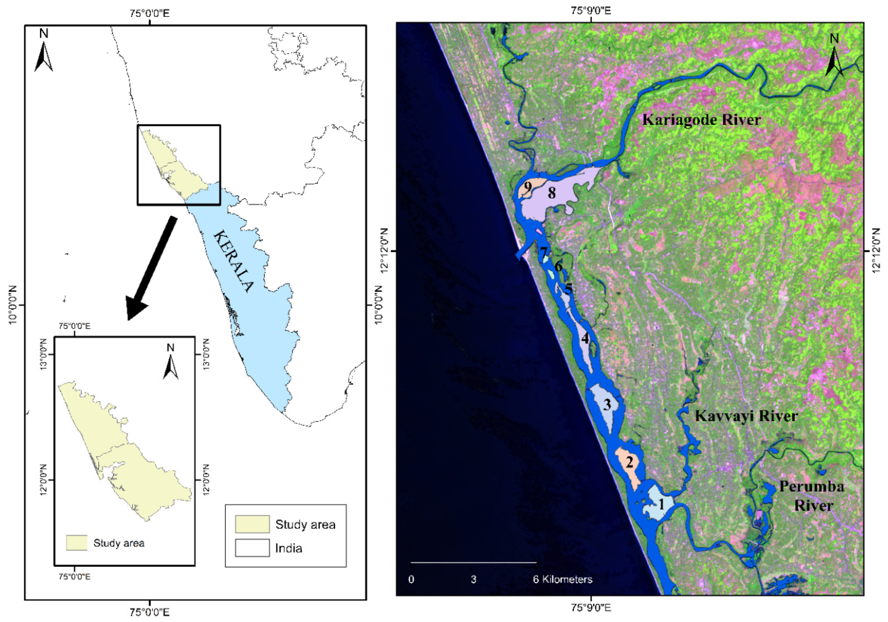
The area selected for the current study is Kavvayi wetland, one of the major wetland ecosystems and the largest one in North Kerala, and it is the third largest wetland in Kerala (
Figure 1). The wetland body stretches from Kavvayi, near Payyanur to Neeleswaram in Kasaragod. It is located geographically 12°2′35” to 12°18’4” N latitude and 75°7′16” to 75°9′57” E longitude. Being located in the humid tropics, the study area has a tropical monsoon-dominated climate with two different rainfall seasons, namely the southwest monsoon (June to September) and northeast monsoon (October–November). More than ~80% of the rainfall in the study area is from the contribution of the southwest monsoon [
20](Abhilash et al. 2019). In addition, the region experiences a higher mean temperature of 36 °C during March to May and a low mean temperature of 28 °C in December–January. The mean wind speed of the study area is 7.7 miles per hour. This region physiographically and geomorphologically falls under fluvial-estuarine factors and is modified because of anthropogenic activities. It is fed by the following five rivers, namely Neeleshwaram, Tejaswini, Erppe, Perumba, and Ramapuram. Barrier islands, sandbars, mud flats, strand lines, mangroves, and tidal flats are the major landforms in the study area. Kavvayi Lake is separated by a sandbar, which lies parallel to the coast at a distance of 21 km. This ecosystem contains 42 species of mangroves, more than 60 varieties of birds, and 39 fish species. In some areas, sandbars have a width of just 50 meters, which makes them delicate areas that need to be preserved and protected. The study area has 68 sacred groves (kavus) in the Kavvayi river basin, some of which are very large and prominent. The change in hydrology of the wetland is controlled by the sea, which plays an important role in regulating the migrant fauna. Therefore, this ecosystem should be treated and conserved by considering its ecological importance. Being located in the coastal stretch, the study area experiences regular storm surges during the southwest monsoon, which plays a significant role in shaping beach morphology. Furthermore, Tsunami of 26 December 2004 in the Indian Ocean severely affected not only southern Kerala but also northern Kerala. A peak tsunami amplitude of 3.0–3.5 m [
21] was reported near to the study area and also had a significant impact on the framing beach morphology.
3. Results and Discussion
3.1. Shoreline Changes Rate Using DSAS
The islands and their shorelines were digitized from four satellite images collected over a period from 1990 to 2014. Even though the entire span of 25 years of satellite imageries-based data was acquired, the entire period was not used. The images were selected based on the coverage of the entire study stretch and interpretability of the data with image clarity free from clouds as well as any other disturbances in image clarity. Based on these criteria among the 25-year period, satellite images of the years of 1990, 2000, 2005, and 2014 were selected. This study utilized three statistical methods (
Table 1) for estimation of shoreline change rates, such as EPR, LPR, and NSM, which are considered to be good indicators to analyze such changes. The results indicated that the study area suffered substantial changes during the selected years.
3.2. Net Shoreline Movement (NSM)
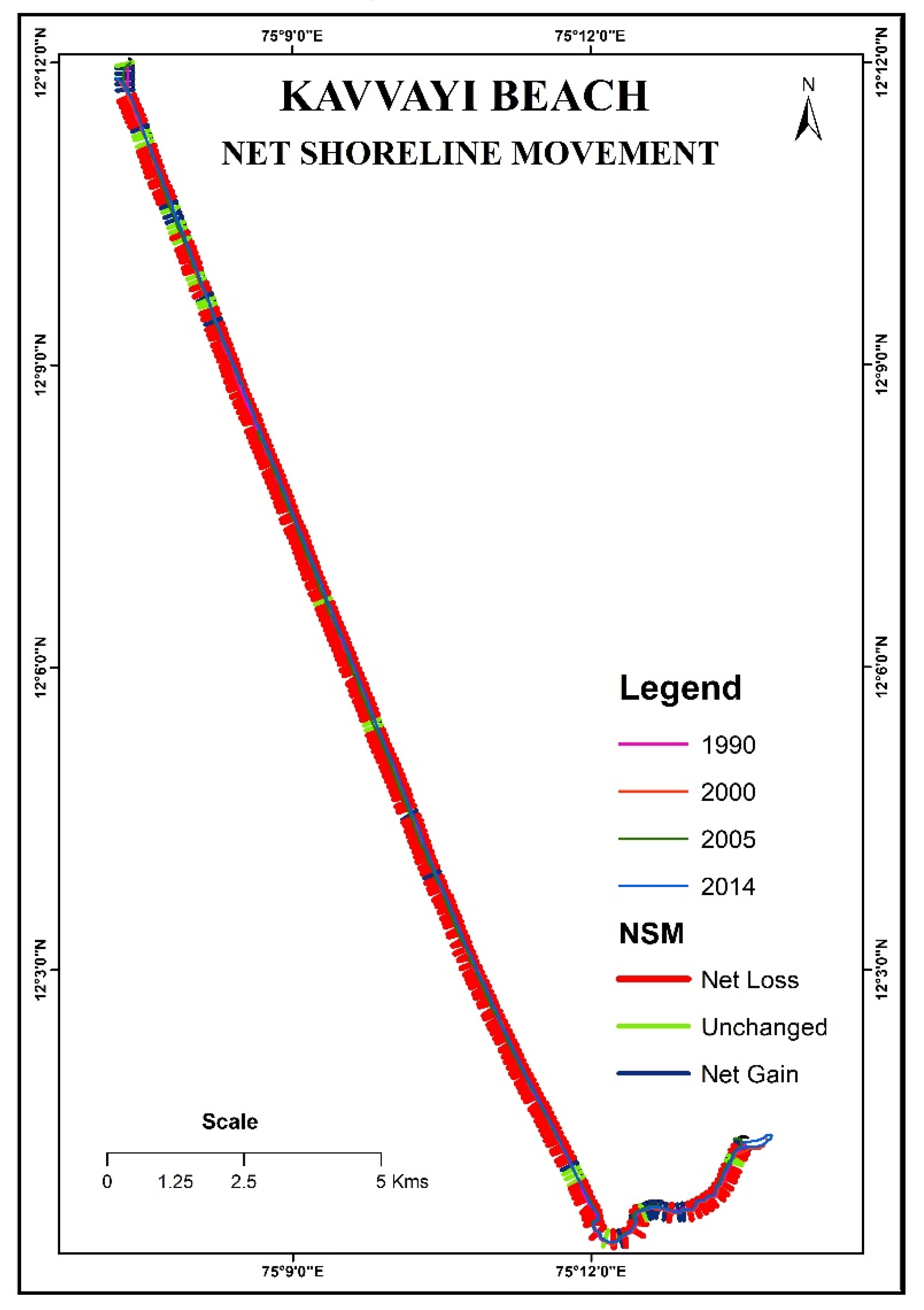
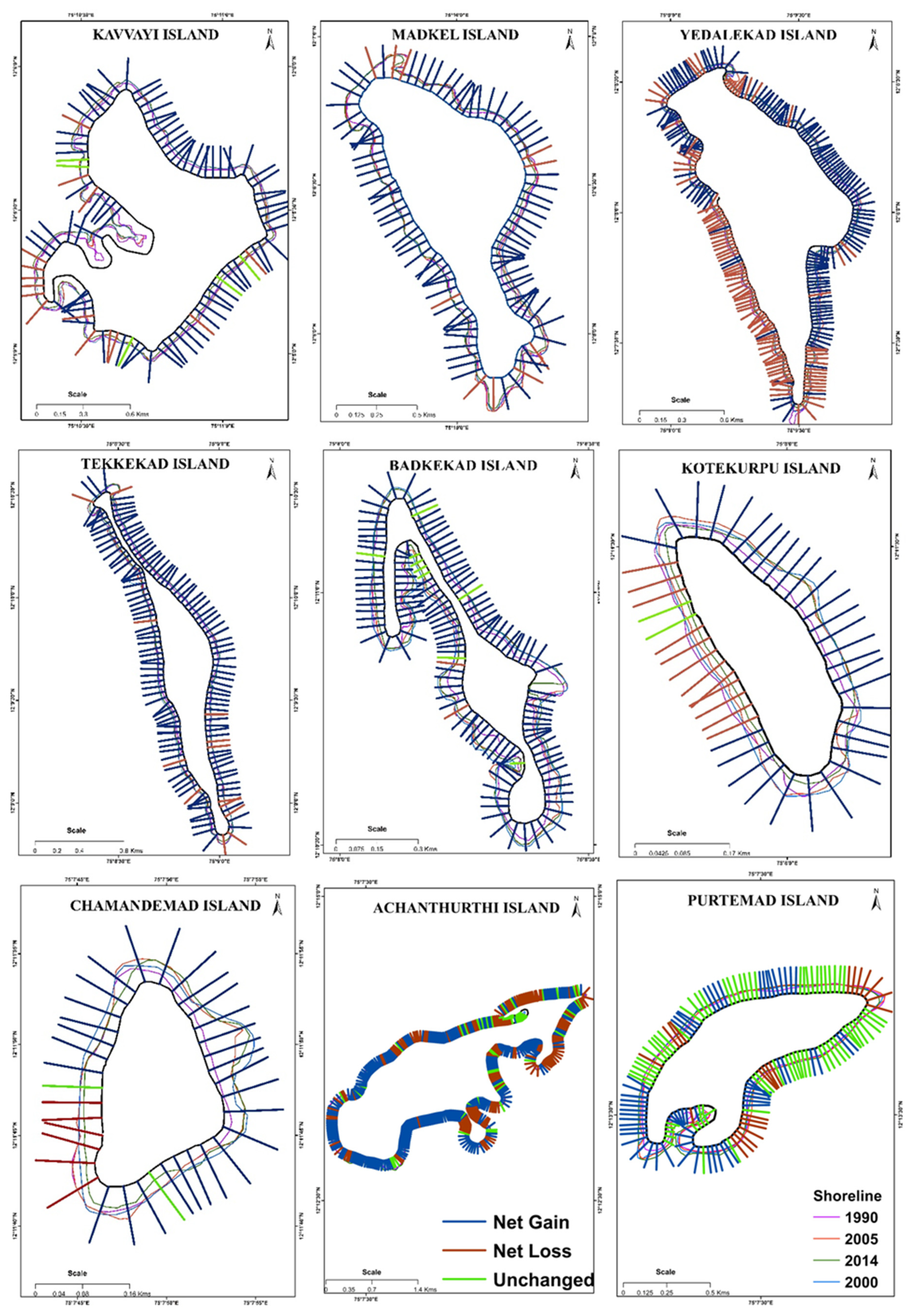
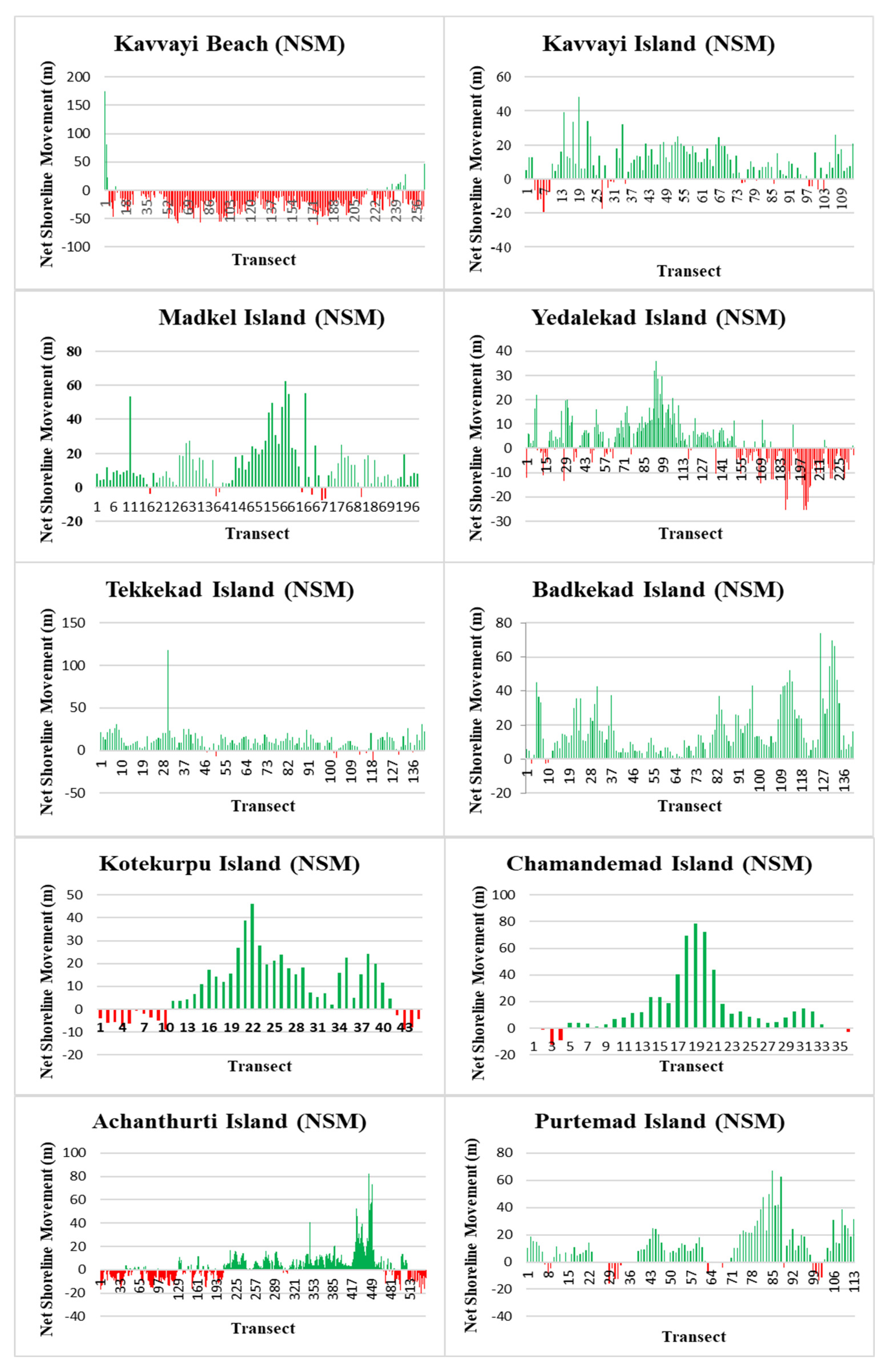
Net Shoreline Movement is the distance between the oldest (1990) shoreline and the most recent (2014) along each transect generated for the study area. The results of NSM rates are given in
Table 1 and
Figure 2,
Figure 3 and
Figure 4. Upon analyzing NSM rates from nine islands and one beach, it can be shown that Kavvayi beach and Achanthurti Island were subjected to erosional processes from 1990 to 2000. Compared to the NSM values for 2005–2014, erosional activity in 1990–2000 was less as the minimum NSM values during 1990–2000 were −53.190 at minimum and 114.240 at maximum, with a mean value of −7.742. The NSM values during 2000 to 2005 were −158.950 at minimum and 65.580 at maximum, with a mean of 9.125.
The shoreline along the Kavvayi, i.e., transects 3–5, 241–245, and 261, had high accretion activities, while all other transects showed low levels of accretion and high erosional activities. During the entire period of study, i.e., 1990 to 2014, it showed marine transgression, as the mean NSM values were observed as −19.580. Thus, it can be noted that Kavvayi beach has moved inward, more land has transformed into a beach, and more land has been subjected to transgression of the sea. During 2000–2005, Achanthurti island showed accretion with a mean NSM value of 1.942 as compared to a mean NSM value of –0.766 for the period of 1990–2000. This trend of accretion was followed later throughout the period of study. The NSM values obtained from 1990 to 2014 are −20.159 at minimum and 82.200 at maximum, with a mean value of 2.521.
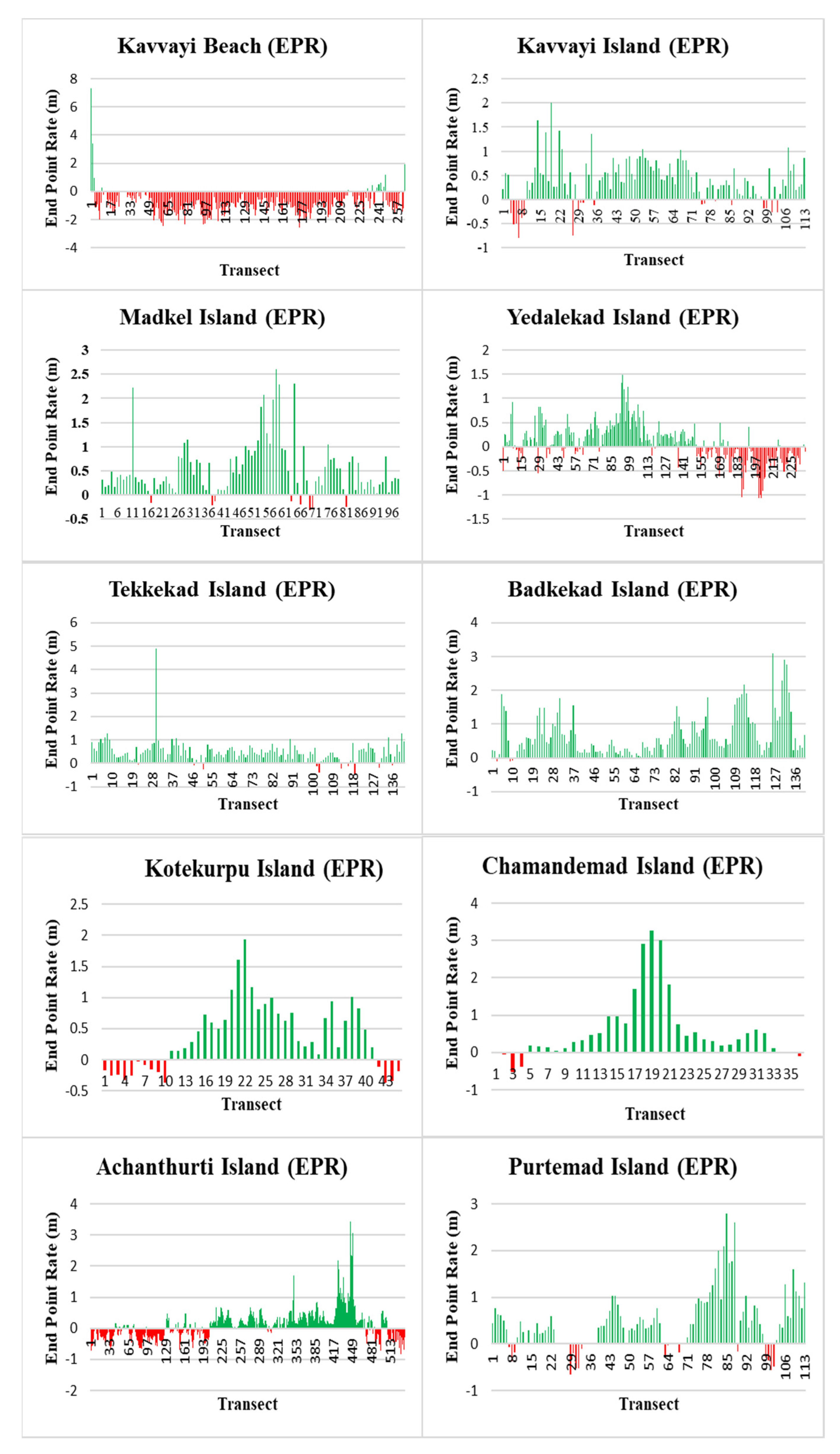
3.3. End Point Rate (EPR)
The EPR is calculated by dividing the distance of shoreline movement by the time between the oldest and most recent shoreline (DASA V.4.3). The EPR rate of Kavvayi beach during 1990–2000 was −5.320 m, and maximum erosion rates were shown during 2000–2005 (
Figure 5). The period of 2000–2005 was observed to be the years with high erosion rate as compared to the rest of the study period. This again asserts the proof for impact on the wetlands and beaches in the wake of the tsunami on 26 December 2004 in the Indian Ocean with a wave amplitude of 5 m.
EPR rates gave insights into observations, which were already obtained from various other DSAS methodologies followed in this study, such as the erosional process being much more concentrated on the western banks of the islands due to factors such as wind and tidal flooding from the Arabian Sea on the western side. It should also be noted that the EPRs were much lower on islands than on Kavvayi beach because islands are located in backwaters and can minimize tidal and wind effects in wetlands. Based on DSAS analysis during 2000–2005, the beach had a maximum erosion value of (−31.810), and Kavvayi (−0.617), Yedalekad (−1.489), Thekkekkad (−0.429), Badkekad (−0.097), and Kotekurpu islands (−1.420) represented negative values in End Point Rate.
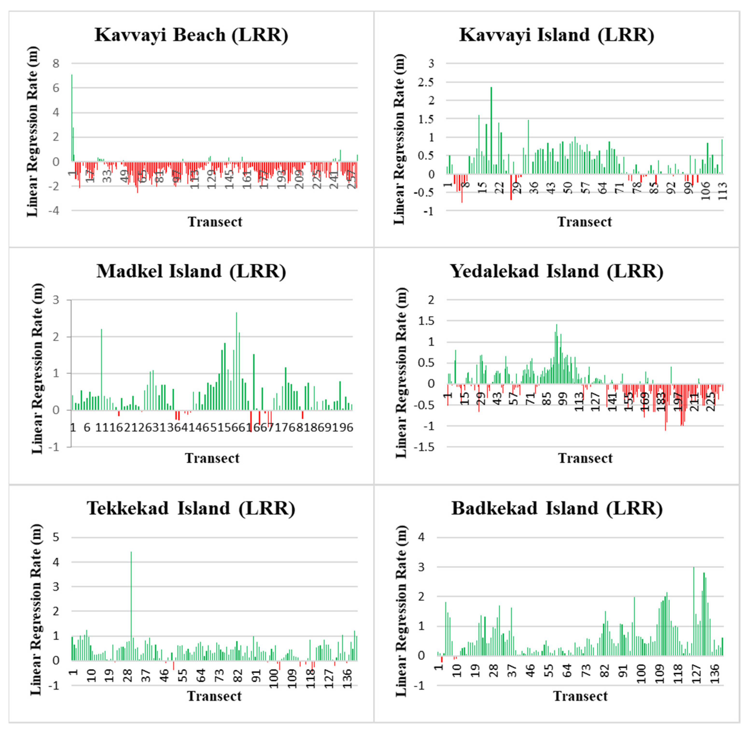
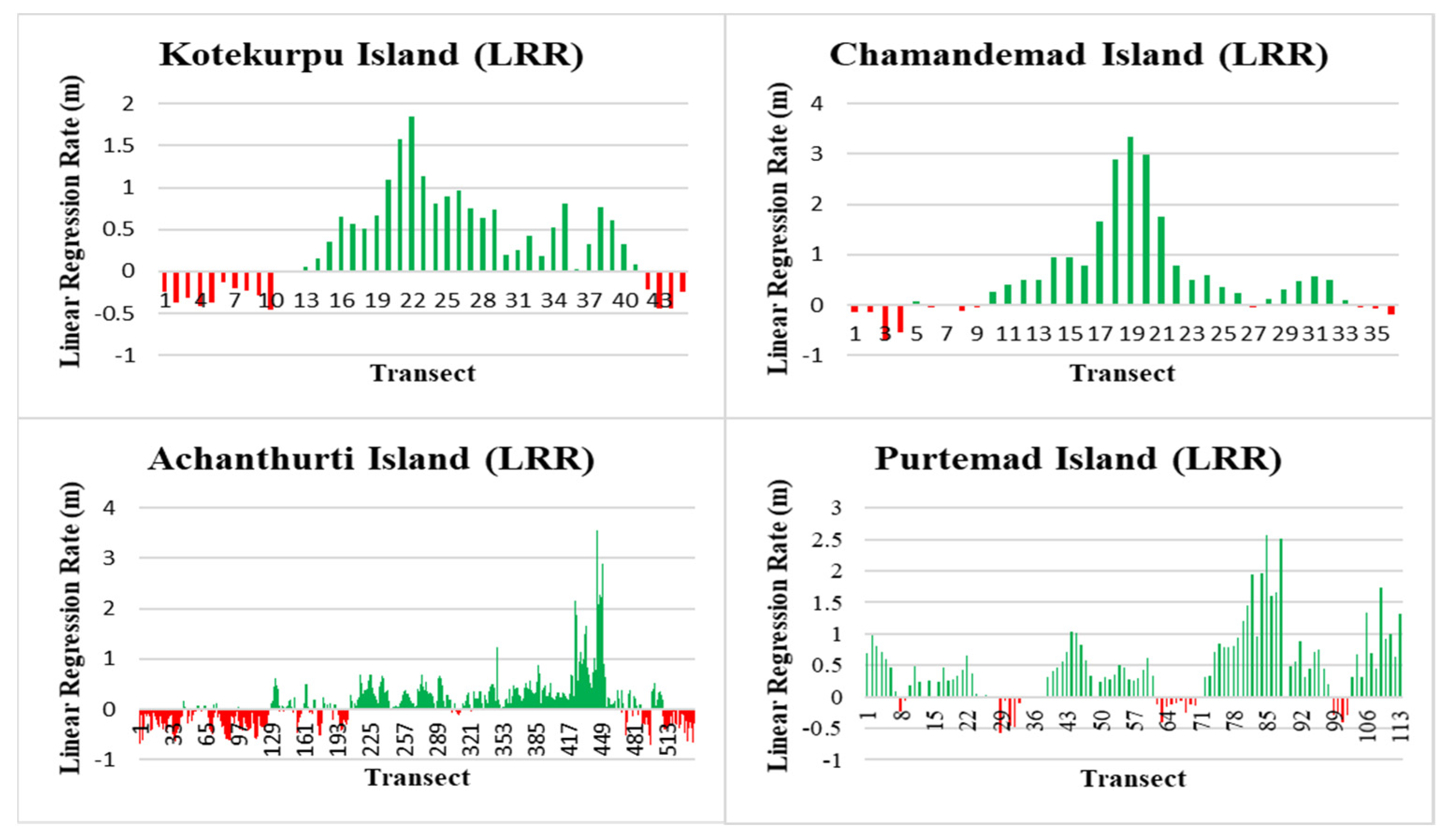
3.4. Linear Regression Rate (LRR)
LRR is used for calculating change rates of shorelines, which consists of fitting a least-squares regression line to multiple shoreline positions for particular transects (Nassaar et al., 2018). A detailed analysis of the linear regression rate (LRR) and the average shoreline change rates for the selected islands is given in
Table 1. Kavvayi beach LRR values showed an LRR of −0.719, showing that the erosion was high in the period of study. All the islands in the study area showed positive values, implicating depositional activity occurring. Out of nine islands in the study area, Yedalekad showed the highest erosion rate, which was −1.120, and the maximum value of LRR was 1.430, with an observed mean value of 0.008, which was the least value identified for all the islands. This was supported by high erosional rates on Yedelakkad Island in the period of 2000–2014. On the other hand, Badkekad Island and Chamandemad Islands showed mean values of around 0.654 and 0.543, respectively, and were the islands with high depositional rates according to LRR (
Figure 6).
The maximum uncertainty using the best estimate for this study was ±0.42 m/year. This indicated that still more accurate and precise methods need to be evolved, and a framework needs to be formulated by considering the uncertainties involved in such exercises. The study revealed that there is a strong need for coastal management plans, which identify such issues of erosion/deposition and how these can be effectively managed. These plans are a useful way for local self-government (LSG) departments to identify the impacts and plan for climate change adaptation and mitigation programs to conserve this coastal ecosystem in their regions.
4. Discussions
This study utilized three statistical methods (
Table 1) for estimation of shoreline change rates, such as EPR, LPR, and NSM, which are considered to be good indicators to analyze such changes. The obtained results indicate that very large amounts of shoreline changes were observed in the selected period for the study. The results showed that the study area suffered substantial changes such as marine transgression and erosion during the period observed. The results are represented as positive and negative variables, which implicate accretional and erosional processes, respectively. The entire Kerala coast that possesses the characteristics of Lateritic cliffs, long beaches, estuaries, offshore stalks, rocky promontories, spits, bars and lagoons, [
27] has a definite influence on these shoreline changes. The extensive lagoons, backwaters, sand ridges, and barrier islands are the indications of a active coast with accretional and erosional (transgression and regression) in the geological past. Several islands showed noteworthy changes in the shoreline, where pronounced accretion and erosion are evident. Most of the islands are subjected to accretional processes and very low levels of erosional processes. However, in the case of Kavvayi beach, a very high rate of erosional activity was observed. As expected, the accretionary process is observed at bare minimal levels. It should be noted that this is caused by tidal forces of the sea and anthropogenic activities in coastal areas. On the other hand, islands in Kavvayi backwater show minimal erosional activity and a high level of accretionary processes. This is justifiable on account of the sedimentary load of the river into the backwaters. That is, the islands are not affected by any tidal forces; they are only influenced by the depositional regime of the river. It can also be noted that the eastern part of the islands shows more accretion than the western parts. This also indicates the depositional activity of the river, as it is flowing east to west. Such studies will help to understand the impact of tidal forces as well as the depositional activity of rivers.
The mean NSM value obtained during 2000–2005 shows a positive anomaly as compared to the rest of the datasets obtained from Kavvayi beach. This can be justified in the wake of the 2004 Tsunami on the western and eastern coasts of the Indian subcontinent and other Southeast Asian countries [
21]. Tsunamis create a substantial exchange of materials from the nearshore zones and shelf to the beach and estuarine environments [
28] as the waves are diffracted, and not a direct impact. It is observed that northern areas of the shoreline of Kavvayi beach show fewer erosional activities compared to other areas of the beach that show dominant erosional activities during the whole series of years from the observed datasets. The breakwaters at the inlet, act as groins, and this might be due to the anthropogenic factors (associated with the construction activities). Thus, significant accretion might have occurred in the northern side due to the dominant northerly longshore currents during fair weather. The shoreline along the Kavvayi has high accretion activities, while all other transects show low levels of accretion and high erosional activities, if we consider different time periods. If we consider the entire period of study (from 1990 to 2014), it showed marine transgression and, hence, it can be noted that Kavvayi beach has moved inward, more land has been transformed into a beach, and more land has been subjected to transgression of the sea.
During the years of 1990–2000, Achanthurti Island showed high levels of erosional activity as it resides on the northernmost island of the Kavvayi backwaters and is situated near to the river mouth. Three sides of the island are exposed to the river mouth coming from inland, and only one side, i.e., the western side, is facing the backwater. Thus, this island shows high levels of erosion on the NE, E, and SE sides of the island and accretion on the western side of the island. From the period of 2000–2005 to 2005–2014, the End Point Rate changed to −8.730 and −3.340 and net shoreline movement changed to −45.730 and −30.050. That means shoreline changes of Achanthurti are influenced by accretion from 2005 due to the construction of a jetty in the study area. Because of this jetty, deposition by the Kariyamkode river is increased (
Figure 1), later leading to the formation of a new small island on the SW side of Achanthurti Island. As described earlier, The breakwaters jetting out into the sea at the inlet, act as groins, ever since the construction started a few years back. This might have resulted in the significant accretion.
In 1990–2000, all islands in the wetlands of Kavvayi showed evidence of accretion, as this can be substantiated by a little movement of water forces in the wetlands; thus, the islands are not subjected to river/tidal forces. For the next period, i.e., 2000–2005, the NSM for five islands showed negative values, which implicates those erosional activities might have happened during that period. These are Kavvayi island (−3.082), Yedalekad island (−7.442), Thekkekkad (−2.144), Badkekad island (−0.486), and Kotekurpu island (−7.096). NSM values for islands in their western parts show erosion and the eastern parts of islands show accretionary behavior. The EPR is calculated by dividing the distance of shoreline movement by the time between the oldest and most recent shoreline (DASA V.4.3); hence, the values may change according to the time period. The EPR rate of Kavvayi beach during 1990–2000 is −5.320 m, and maximum erosion rates are shown during 2000–2005 (
Figure 5). The period of 2000–2005 is observed to be the years with high erosion as compared to the rest of the study period. This again asserts the proof for the impact on the wetlands and beaches in the wake of the tsunami on December 26 2004 in the Indian Ocean with a wave amplitude of 5 m.
The changes occurred in these coastlines might be explained due to the Tsunami energy, which might have determined the wave amplitudes due to convergence and divergence of energy from Helmholtz resonance in harbors, bathymetry, interaction with the tide, quarter-wave resonance amplification, and reflections from the Lakshadweep Islands and from distant coastlines of Somalia in Africa. This can be further explained with the various physical oceanographic processes such as boundary reflections, constructive interference, interaction with the wind wave, coupling with internal waves due to ocean density gradients, and tidal effects [
21]. That study also confirmed that that tsunami waves alone might not contribute for the direct observed maximum amplitudes, while in few locations in the study area, local resonances and zones of convergences might have amplified it. The times of occurrence of the higher amplitudes showed that the waves played significant role which might be from the Lakshadweep Islands and even from the Somalia coast on the African continent. The effect of the reflected waves during Tsunami period was more visible on the northern coast of Kerala than on the southern part [
21].
Framework for Development of Integrated Coastal Zone Management
The study revealed that there is a strong need for coastal management plans, which identify such issues of erosion/deposition and how these can be effectively managed. These plans are a useful way for local self-government (LSG) departments to identify and plan for climate change impacts and its adaptation and mitigation management plans in their regions. Coastal zones are thickly populated natural environments and dynamic in nature and the livelihood of many people depends on these ecosystems; hence, it is essential to plan for effective coastal zone management actions. In general, the management of accretion and erosion in coastal zones has been reactive, while long term plans are rare. However, in recent years, because of climate variability and climate extremes, management plans are progressively proactive and considerate of longer duration into the future, while devising appropriate adaptation responses for coping. This is evident from the shoreline management plans of the UK, Netherlands, etc., which look at the timescale of 100 years [
29,
30,
31].
Coastal erosion has three potential adaptation strategies, i.e., protect, accommodate, and retreat as per the IPCC Coastal management strategy, and it very well fits into the Integrated Coastal Zone Management Plan (ICZMP) of the Government of Kerala [
28,
29,
30,
31]. The study revealed that areas in these Kavvayi wetlands are vulnerable zones and, hence, priority needs to be given to those areas, as these have a large number of economic activities and are related to their livelihoods too. The strategy of protection can be either soft or hard engineering solutions such as dykes, artificial dunes, beach nourishment/, etc). Soft engineering protection involves providing coastal defense by adapting to the requirements and enhancing natural environments, by supplementing the natural processes. The advantages of these soft techniques are that they are reversible, give flexibility, and allow the policymakers to opt for a wide range of shoreline management plans (SMPs). In the case of accommodation strategy, the vulnerable areas that we have identified can be retained with the current land use and restoration of wetlands near to the shore; however, other new constructions could be avoided or an attempt could be made to change the construction with the least disturbances, improving the preparedness at the same time, and this will hold good for accretion. In the case of retreat, existing buildings can be abandoned, and inhabitants that need to be resettled require new areas far away from the shore to combat such erosion.
Seawall/revetments, sea dyke, groynes, detached breakwaters, storm surge, barrier/closure dams, land claim/raise land areas, beach nourishment, dune construction, coastal aquaculture, floating agriculture, growing of salt-tolerant erosion-resistant crops, managed realignment, etc., are some of the technologies available as an adaptation option to these areas for managing the coastal erosion [
32,
33,
34,
35]. As per the field observations, the vulnerability of these coastal zones largely depends on theexisting management activites as well as their socio- economic and cultural conditions. The technologies that have been discussed earlier will be most effective when executed as part of a wider integrated coastal management (ICZM) framework. There may be blocking barriers for effective implementation; however, this can be overcome by the provision of technical support and guidance from research organizations, academic institutes, non-governmental organizations (NGOs), commercial organizations’ coastal decisionmakers/policymakers, and other stakeholders’ involvement in a holistic way, which would greatly aid effective adaptation. This ICZM can act as a platform for co-creation by considering the different range of available adaptation options to choose the best management strategy and for educating and engaging the stakeholders.
5. Conclusions
This study attempted to evaluate the morphological changes in shoreline and coastal islands of Kavvayi wetlands of humid tropical Kerala, India. The study showed that the DSAS methodology is highly apt for shoreline vulnerability assessment from data observed from various satellite images collected during the study period of 25 years, even though a few uncertainties were present. The results confirmed that Kavvayi beach was subjected to high levels of erosion during the entire period of the study, as opposed to that of the islands in the Kavvayi wetlands, which is evident through visual observation being too different from the indicators such as EPR, NSM, and LRR. The Net Shoreline Movement of Kavvayi beach showed high rates of erosion in the periods of 1990–2000 and 2005–2014, with the latter being more erosive on the beach. The period of 2000–2005 had a positive mean value, implicating accretion on the coast, which can be explained in the wake of the 2004 Indian Ocean tsunami. A tsunami moves sediments from the shelf and nearshore zones to the beach as the waves are diffracted, and it might not be a direct impact. Thus, by comparing these three periods of studies, it can be established that Kavvayi beach has been subjected to marine transgression over the period. Out of the nine islands in the wetlands, Achanthurti Island has also been subjected to erosion, but on a lower scale compared to that of Kavvayi beach, as it is in a wetland. Three sides of Achanthurti Island are surrounded by the river mouth, which is the main cause of erosion on this island. During the period of 2000–2005, five islands in the Kavvayi wetlands were subjected to erosional processes, situated on the western banks, and accretion on the islands on the eastern bank. For the rest of the period of study, all islands showed high depositional rates. These higher depositional rates are justifiable based on low tides and aeolian effects on the islands, as they are situated in wetlands. Coastal management plans based on the study have been discussed and the ways and methodologies for developing an Integrated Coastal Zone Management and its framework were also discussed. The limitations of the study are that there are uncertainties that need to be minimized for better precision on the assessment of shoreline changes, which can be achieved by field verifications in later stages, when such databases are created on long-term bases. This study will help to derive future policy directions to foster a comprehensive and systematic approach to conserve these precious resources from further degradation in the wake of climate extremes.

 ,
, 


