
Determination of Seasonal Indices for the Regionalization of Low Flows in the Upper Vistula River Basin

Faculty of Environmental Engineering and Land Surveying, University of Agriculture in Krakow, al. Mickiewicza 21, 31-120 Krakow, Poland
*
Author to whom correspondence should be addressed.
Water 2023, 15(2), 246; https://doi.org/10.3390/w15020246
Submission received: 1 December 2022
/
Revised: 27 December 2022
/
Accepted: 3 January 2023
/
Published: 6 January 2023
(This article belongs to the Section Hydrology)
Abstract
:Low flow is a parameter that is used for many purposes in water management. It is particularly important in terms of the needs of small water supply systems, which usually are located in ungauged catchment areas. The aim of this study is to determine the values of seasonality indices for the regionalization of low flow characteristics in the Upper Vistula river basin. This study analyzed three seasonality indicators (seasonality index—SI; seasonality histograms—SHs; and seasonality ratio—SR) in 32 selected catchments differentiated in terms of selected physiographic and meteorological characteristics. Daily flows, from the years 1951–2016, were used in the study. On the basis of the analysis, regions characterized by similar values of seasonality indicators were delineated. The non-hierarchical method of cluster analysis, i.e., the K-means method, was used for this purpose. For each region, obtained by this method, regression models were determined using stepwise regression analysis. Three groups of low flow occurrences were determined: winter, summer and mixed. The delineation of an additional mixed group for the Upper Vistula river basin resulted in a much better fit of calculated flows to observed values than in the case when only two groups of low flow seasonality were determined (winter and summer).
1. Introduction
Low flow is the parameter that is most frequently used for many purposes in catchment water management. This value is needed for determining permitted water transfers, irrigation systems and when planning water supply for settlements. Low flow characteristics are also needed in water management for water intake permits, the discharge of treated wastewater and the associated location of wastewater treatment plants [1,2,3]. Another important aspect of the use of this parameter is the determination of environmental flows for the protection of wildlife or for hydropower purposes. Increased demand for water during periods of low flow may increase water deficits. [4,5,6]. In addition, the application of the Water Framework Directive requires the estimation of low flows to assess good state of water bodies [2]. As pointed out by [7], rivers characterized by a rainfall-dominated discharge (e.g., the south of France, southwest England, Central Europe) will be prone to droughts in the future. The opposite situation will occur for catchments with a flow regime induced by melting snow [7]. The magnitudes and seasonal timings of low flows vary between geographic regions [8]. Low flows should be considered taking into account many factors that influence them, such as soil infiltration characteristics, hydraulic characteristics, aquifer extent, rate, the frequency and magnitude of recharge and evapotranspiration, but also land cover, topography and climatic factors [9,10,11]. On a regional basis, determining the spatial variation of low flow is important not only for controlled, but also uncontrolled, watercourses [12]. This is an issue of particular relevance to water management and especially for small water supply systems for which there is a need to develop a project for water intake. The water intakes for such systems usually take water from watercourses located in ungauged catchments. In Poland, and in many countries, there is a need to search for the methods of estimating low flows in ungauged catchments.
Many existing water intakes have become insufficient for the needs of the population. In order to develop a concept or a water supply permit, it is necessary to have hydrological information on low flows, which is particularly difficult for small systems as they are located in ungauged catchments. Limited water retention capacity in a catchment area can worsen the effects of drought, thus managing water resources in such areas will become a major challenge. Therefore, the knowledge of the occurrence of drought periods allows better preparation for the occurrence of such phenomena [7]. Additionally, assuming population growth and changing water consumption patterns, an increase in water demand is expected, which could lead to conflicts over water [13]. An important issue in the analysis of low flows is the seasonality of their occurrence. This is important in relation to the assessment and monitoring of the hydrological regime of rivers, as well as the impact of climate change on low flows [14,15]. As a result of climate change, it is estimated that future catchments of different scales in Central Europe, e.g., the Upper Rhine, will experience a regime shift from the winter low flow regime to the summer low flow regime [16,17]. At the same time, [16] indicates that as a result of a warming climate, the variability in the timing of lows will decrease, making drought a more predictable phenomenon. In the case of a seasonal climate, with warm and cold seasons occurring, low flows are influenced by various processes so that the annual series of extreme values are a mixture of summer recessions and winter freezes. Because of the fundamental differences of summer and winter processes, regionalization may take advantage of a separation of summer and winter low flows [18]. Schreiber and Demuth [19] analyzed the seasonality of the annual mean 10-day minimum MAM(10) of total runoff in catchments in southwestern Germany. The analysis was performed for 10 regions and for the entire study area. Aschwanden and Kan [20] conducted a Q95 analysis for a catchments in Switzerland. In the United States [21] analyzed river headwaters and noted an identified distinct variability pattern in the frequency of low flow days. Based on their analysis, they identified three clusters in which low flows occurred mainly during summer and early autumn. They found that in the western case, a precipitation deficit played a role in the occurrence of low flows, while in the central and western regions, which are characterized by dense vegetation, low flows occurred mainly during summer and autumn. This was related to increased evaporation during the summer season [21]. Another example of low flow analysis is the study by Dingman and Lawlor [22], conducted for the Vermont and New Hampshire region. Fangman and Haberlandt [23] studied low flow seasonality in the federal state of Lower Saxony, situated in northwestern Germany. A detailed analysis of the seasonality of low flows was carried out by Laaha [24] and Laaha and Blöschl [25,26]. They conducted such an analysis for low flows q95 in 325 small catchments, located in Austria. They used seasonality histograms (SHs), seasonality index (SI) and seasonality ratio (SR) in their analysis. As a result of this study, they divided the catchments into 10 groups and classified them into summer or winter subregions. Similar analysis was made by Vezza et al., 2010 [12], who used, similarly to Laaha and Blöschl [25], three seasonality indices for low flow regionalization for catchments located in the northwestern Italy. Vlach et al. [17] analyzed the long-term variability and seasonality of low flows and streamflow droughts in fifteen headwater catchments of three regions within Central Europe. In their analysis, SI and SR indices were used.
In Poland, one of the first analysis of seasonality was carried out by Rotnicka [27]. She attempted to identify the so-called hydrological season, i.e., a sequence of days in a year characterized by relative similarity of the magnitude, dispersion and character of water levels. Additionally, Jokiel and Tomalski [28] determined the hydrological seasons of annual flow hydrograms for selected rivers located in central Poland. In another study by Jokiel and Stanisławczyk [15], the authors analyzed the changes and long-term seasonal variability of outflow for catchments located in different parts of Poland.
The estimation of low flow characteristics in the case of a gauged catchment is carried out using direct statistical methods [29]. The issue concerns ungauged catchments, where hydrological information is often needed for different water management purposes, e.g., for water supply. Hence, there is a need to develop methods to determine low flow in such catchments, taking into account long hydrometric and meteorological measurement series.
The aim of the study is to determine the values of seasonality indices for the regionalization of low flow characteristics in the Upper Vistula river basin. As a predictive model, a stepwise multiple regressions based on physical catchment characteristics and seasonality indices was used. The results of the studies can be used to estimate q95 flows in ungauged catchments and also, in practice, for modernization and design of new water intakes for small local water supply systems. Additionally, it should be added that the presented analyses are innovative, both with regard to Poland but also with reference to international reports, which are limited.
2. Materials and Methods
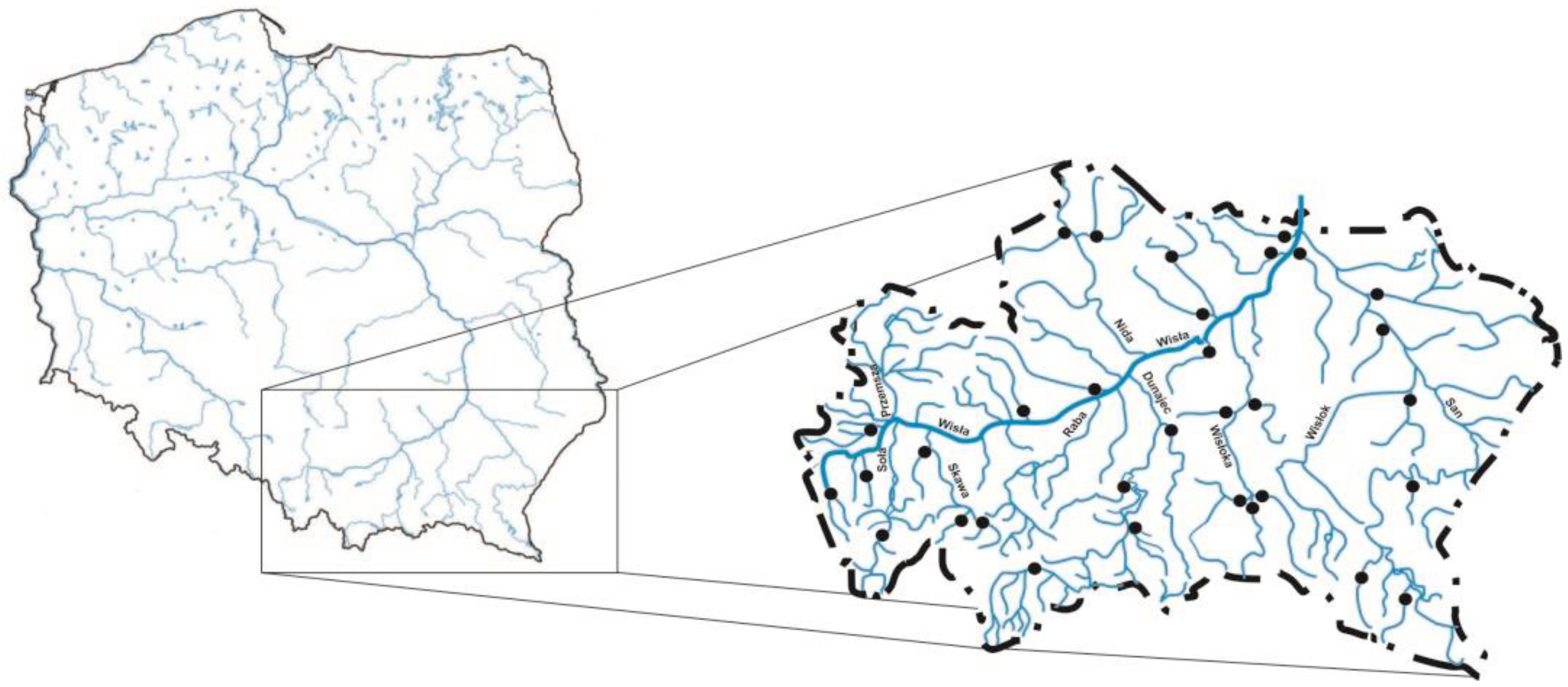
The study was performed in 32 selected catchments belong to the Upper Vistula basin (Figure 1). The source material for the analysis was time series daily data from the period 1951–2016 (Table 1). It was assumed, as a criterion of catchments’ selection, that for analysis only those areas in which daily streamflows were available with a minimum record length of 20 years were utilized. In the analysis, 12 physiographic and meteorological characteristics of catchments were also used (Table 1).
The following physiographic and meteorological parameters of the catchment were used (Table 1): length of the watercourse (L), catchment area (A), mean annual precipitation (P), mean catchment slope (I), land use (U) and soils (S).
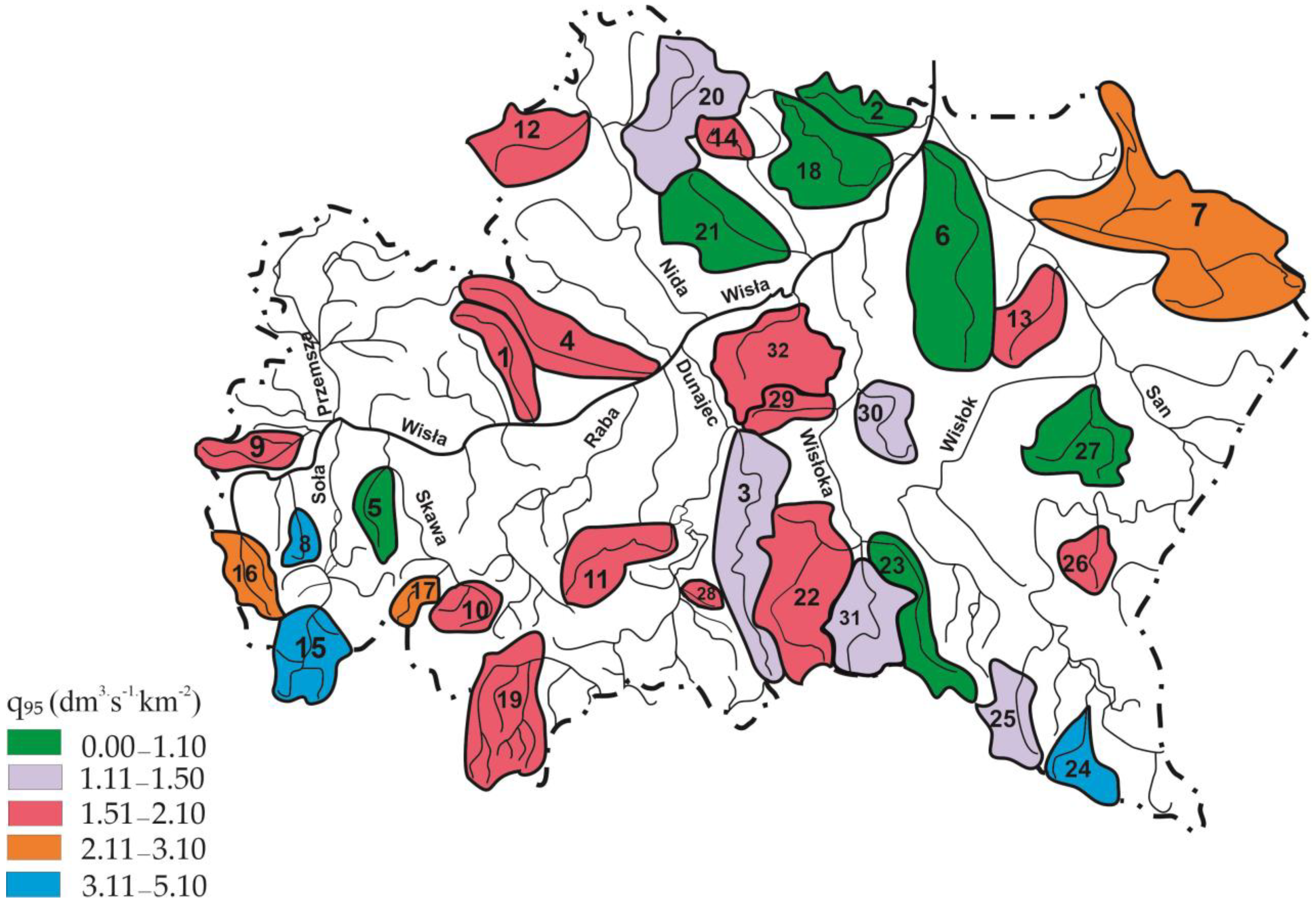
The analysis was performed for a Q95% flow quantile, i.e., a flow that is equaled or exceeded on 95% of all days within the observation period. This characteristic was chosen because it is relevant to many aspects of water management, such as design of water supply systems, and is widely used in Europe. Then, Q95% was subsequently standardized by the catchment area, obtaining unit specific low flow discharge q95 dm3∙s−1∙km- 2. A map of specific low flow discharge q95 dm3∙s−1∙km−2 for the analyzed catchments of the Upper Vistula river basin is presented in Figure 2.
Time series of daily data and precipitation were obtained from the Institute of Meteorology and Water Management, National Research Institute in Warsaw. Parameters related to morphometry and landform were determined on the basis of Kondracki [30] and soils, land cover and catchment development were determined on the basis of the soil map of Poland [31] and Corine Land Cover 2012 [32].
Physiographically, the area of the Upper Vistula basin, where the analyzed catchments are located, is situated within three large Carpathian physiographic units: Carpathians, Subcarpathian valleys and Małopolska Upland. The area of the Carpathians and the Upland is the area where most tributaries of the upper Vistula have their sources, while the Subcarpathian valleys are the transit area for the Vistula and the estuary area for the rivers and streams formed in the Subcarpathian and the Subcarpathian Upland [33]. Additionally, in terms of geological structure, the basin area is diversified [34], which translates into a diversity of soils in the area. Four types of relief can be distinguished in this area: mountain, upland, foothill and lowland.
For the analysis, catchments differentiated in terms of physiographic parameters were taken (Table 1). The smallest catchment area is 66.3 km2 and the largest is 2034 km2. Additionally, the mean slope of the catchments varies from 0.002 for the Pszczynka and Łęg catchments to 0.091 for the Biała catchment (Table 1). The selected catchments are also diversified in terms of land use. They are dominated by arable land, which ranges from 7.4% for the Łęg to 87% for the Szreniawa, and forests, which constitute from 3% (Szreniawa) to 67.60% (Skawica).
The methods applied in this study are similar to those used by Laaha and Blöschl [25] and Vezza et al. [12]. Three seasonality indices were used to determine the seasonality of the occurrence of specific low flow discharge q95: a seasonality ratio (SR), a cyclic seasonality index (SI) and seasonality histograms (SHs).
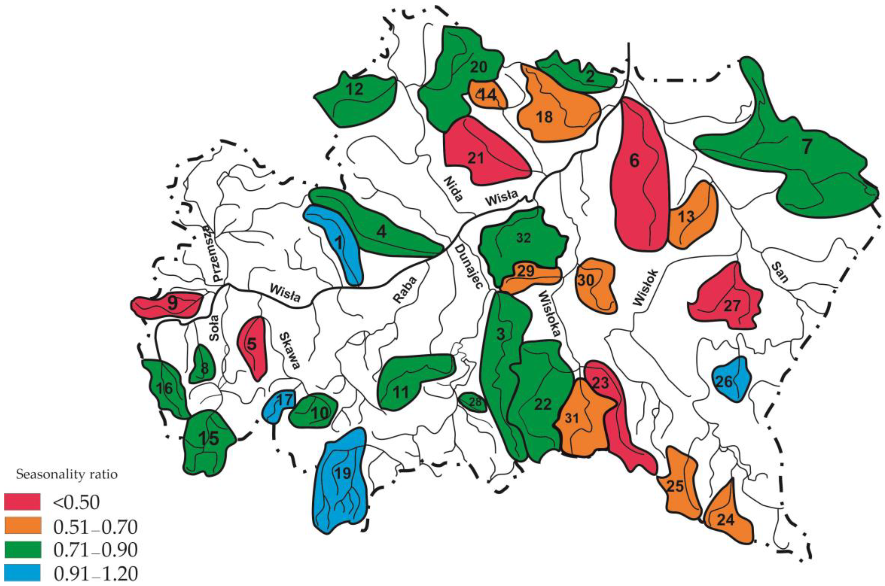
The seasonality ratio (SR) representing the ratio of summer (q95s) to winter low flow characteristics (q95w) is given in Equation (1) [26]. First, daily discharge data were divided into summer discharge series, from 1 May to 31 October, and winter discharge series, from 1 November to 30 April, in order to differentiate summer low flows caused by precipitation deficit and winter low flow events caused by snow accumulation and frost in highland and mountain areas [17]. Then, from summer and winter discharge time series data, the characteristic values of q95s and q95w were calculated for each catchment.
SR values > 1 indicate the presence of a winter low flow regime, whereas SR values < 1 indicate the presence of a summer low flow regime.
Another parameter analyzed was the seasonality index, SI. This index is similar to the one used by Burn [35], Young et al. [36] and Laaha and Blöschl [26]. The SI is a parameter on the basis of which it is possible to determine the average number of days of low flow intensity. The index also shows how strong this relationship is. The index is based on two parameters, Θ and r, which are calculated from the Julian dates of all days of the observation period when discharges are equal or lower to Q95. The parameter Θ represents a measure of the average seasonality of low flows by the average day of low flow occurrence in radians. The value of the parameter ranges from 0 to 2π, where Θ = 0 relates to 1 January, relates to 1 April, π relates to 1 July and relates to 1 October. For each catchments, the days when the flow was less than Q95 were taken for further analysis and then were transformed into Julian dates Dj [17,26].
Dj is the day of the occurrence, when flows are lower than Q95.
In turn, the parameter r is the mean days of occurrence and describes the seasonal variability of low flows and it is dimensionless indicator. Its values range between 0 (low seasonality and means that all low flow events are uniformly distributed over a year) and 1 (strong seasonality and means that all low flow events occurred exactly the same day of the year) [17,26].
The seasonal concentration index r is calculated as Equation (3) [26]:
where:
xθ and yθ are the arithmetic mean of Cartesian coordinate of a total of n single days j and are calculated as Equation (4) [26]:
Lastly, seasonality histograms (SH) were analyzed, which allowed for a more detailed analysis of the seasonality distribution of low flows [26]. The histograms provide complementary information to the seasonality index (SI) and from these it is possible to identify which months are affected by low flow and to determine the shape of the seasonal distribution, whether it is, for example, multimodal or skewed. In the case of this parameter, the shape of the distribution depends on all days when the discharge of a catchment falls below the threshold Q95 [26].
A non-hierarchical cluster analysis method, the K-means method, was then used to determine groups of catchments similar in terms of the seasonality of low flow occurrence. Euclidean distance was used as a measure of distance between clusters.
In the next stage of the analysis, groups of catchments similar to each other due to seasonal occurrence of low flows were determined. For this purpose, the non-hierarchical cluster analysis method (K-means method) was used. Euclidean distance was used as a measure of distance between clusters.
In the final stage of the study, regional models were developed in the form of a multiple regression equation (Equation (7)), in which the dependent variable was low flow characteristics and the independent variables were morphoclimatic parameters of the analyzed catchments [29].
where:
q95 = β0 + β1 · x1 + β2 · x2 +⋯+ βp−1 · xp−1
xi—morphoclimatic parameters of a catchment,
βi—regression coefficient.
Multiple regression analysis identified the parameters that most strongly influence low flows. The best results were obtained using stepwise regression, using Mallow’s Cp coefficient as an optimality criterion [25].
The following assumptions were made for the regression model: the absence of multicollinearity, homoscedasticity and normality of residuals. It is important to check multicollinearity to see whether the independent variable is highly correlated with one or more of the other independent variables in the multiple regression equation. The presence of multicollinearity makes statistical inference less reliable. Another parameter, homoscedasticity identifies dissimilarities in a population. Any variance in a population or sample that is not even will produce results that are skewed or biased, making the analysis incorrect or worthless. Checking the normality of residuals is crucial and is one of the main assumptions of a linear regression model. If the residuals are not normally distributed, then model inference (i.e., model predictions and confidence intervals) might be invalid. The absence of multicollinearity was checked using the variance inflation factor (VIF), normality of residuals using the Anderson–Darling and Shapiro–Wilk tests and diagnostic plots. White’s test was used to check the homoscedasticity of the residuals.
The coefficient of determination R2 for significance level = 0.05 and the adjusted coefficient of determination R2adj (Equation (8)) were calculated in order to determine the consistency of calculated values with observed values.
where:
R2—coefficient of determination,
N—number of predictors,
p—total sample size.
In addition, the coefficient of determination R2cv was determined using leave-one-out cross-validation, which is described in Equation (9). This was applied in order to avoid the so-called error of the third kind and to select the best forecasting model [25].
where:
Vcv—is the average residual square error and is calculated with Equation (10) [25],
var(q95)—is the spatial variance of the observed specific low flow.
where:
—is the estimated value of the i-th dependent variable obtained using a model estimated with all observations except i-th,
—is the observed value.
The root mean square error (RMSE) [38] for each cluster and for cross-validation (RMSEcv) was also calculated. RMSE values equal to 0 indicate a perfect fit.
3. Results and Discussion
The values of the seasonality index (SR), classifying the seasonality of low flows for the analyzed catchments located in the Upper Vistula river basin, are presented in Figure 3. On the basis of the index threshold value equal 1, summer and winter low flows can be distinguished. It was found that in most catchments of the upper Vistula river basin (28 catchments), summer low flows dominate in the analyzed period. In the case of four catchments, Skawica, Dłubnia, Dunajec and Stupnica, SR values were higher than 1, which indicates the dominance of winter low flows.
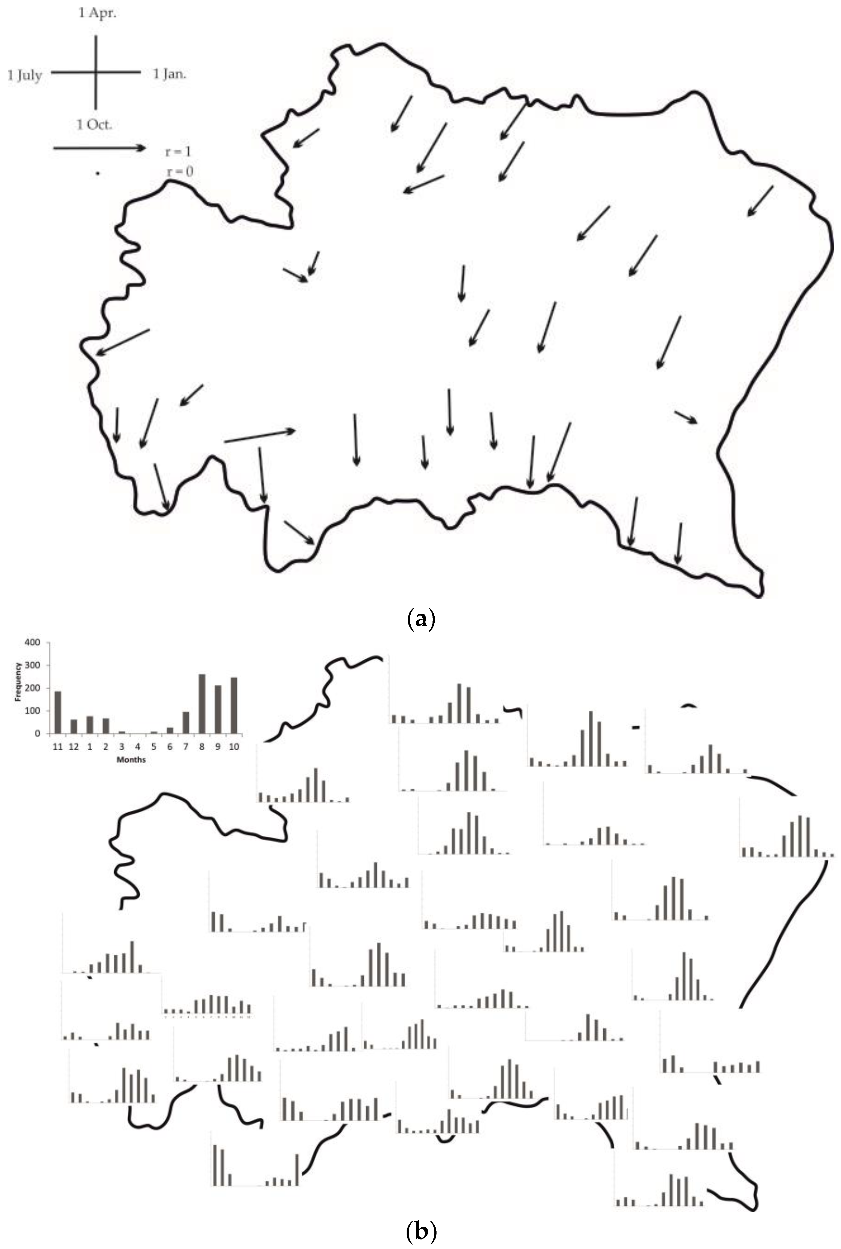
Another parameter analyzed was the SI seasonality index. The results are presented in Figure 4a. The analysis of SI values for the analyzed catchments showed that in the case of the analyzed catchments low flows occur in two seasons: in summer, in twenty-eight catchments, and in winter (January–March), only in four catchments. Summer low flows already occurred from mid-July. Low flows dominated in August and September (10 catchments each), which is related to high air temperature and high evaporation. These results are similar to those obtained by Raczyński and Dyer [39], who determined the seasonal variability of low river stages in south-eastern Poland and found that the maximum frequency of occurrence of low flows occurred in early August. Analyzing the strength of variability of low flows in the analyzed catchments, according to Guilford’s classification [40], it can be noted that strong variability (0.7 < r < 0.9) was observed in three catchments (Mleczka, Czarna and Jasiołka). In contrast, weak variability (0.1 > r > 0.3) was observed only in the Szreniawa catchment. In the remaining 28 catchments, the variability of low flows was assessed as medium. These results are similar to those obtained by Jokiel and Stanisławczyk [15], who studied seasonality indices in catchments located in different regions of Poland and on the Carpathian rivers. They obtained seasonality indices higher than 50%. Kohnová et al. [41] analyzed the seasonality of the occurrence of low flow Q95 for Slovak catchments. The study included 198 small and medium-sized catchments from across the country. Similarly to the study carried out in the paper, summer lows were observed mainly from August to October. However, low flows for August were dominant in catchments located in the mountainous parts of Slovakia. The magnitude of the seasonal concentration index (r) was higher than that obtained by the authors of the paper. For summer low flows, it ranged from 0.8 to 0.95 in 84% of the analyzed catchments. On the other hand, winter low flows were observed from December to March for the catchments located in the central and eastern part of Slovakia. Of these low flows, those occurring in January were predominant. Additionally, for this type of low flow, high values of r were observed, which ranged from 0.8 to 0.9 for most of the catchments.
The SI results obtained by the authors of this paper are similar to those based on SH and SR, thus confirming the type of seasonality observed in the analyzed catchments of the Upper Vistula river basin. For all analyzed seasonality indices, the occurrence of seasonality of winter low flows concerned the same catchments. Knowledge of low flow seasonality is an important aspect during the planning, as well as during the operation of surface water intake. The results show both spatial and temporal variability of low flow, which are important for administrative decisions on the development and management strategy of an area. Water availability, represented by low flows, is used to define the water permit limit for water withdrawal as a tool for water management and planning [13].
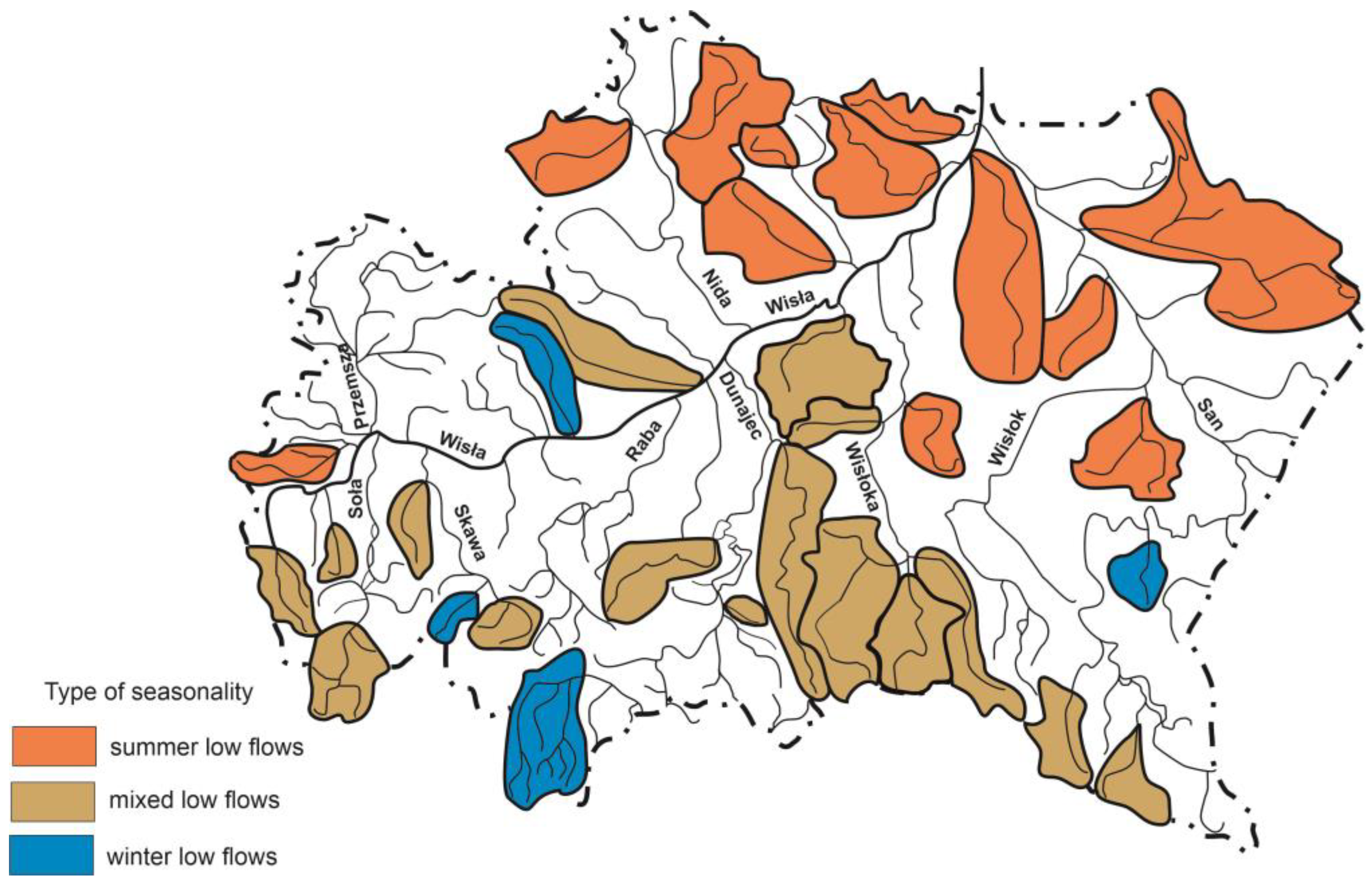
The seasonality histograms (SH) (Figure 4b) were analyzed to determine in which month of the hydrological year low flows occur. On this basis, a map of the analyzed catchments with the dominant type of low flows was created (Figure 5). Analyzing the histograms, it can be seen that for 28 catchments, summer low flows dominate. However, on the basis of a more detailed analysis of the histograms, catchments of mixed type can be distinguished, where summer low flows dominate but winter low flows also occur (nine catchments of mixed low flow type). As far as winter low flows are concerned, their occurrence is observed in four catchments, whereas in three catchments, despite the dominance of winter low flows, autumn low flows occurring towards the end of the hydrological year are also observed, mainly in September and October. Seasonality histograms for the analyzed catchments practically coincide with the type of low flows determined from the SR coefficient.
In a study by Schreiber and Demuth [19], carried out in 169 catchments located in Germany, the seasonality of low flow—MAM(10)—was recorded in practically every month of the year. However, the lowest flows are observed in late autumn, especially in September and October, for most catchments. Vezza et al. [12] analyzed different grouping methods, due to low flow characteristics q95, for 41 catchments in northwestern Italy. For this area and the three seasonality indices used, they found that, for Italian catchments, the division of low flows into two seasonality groups (summer and winter) best reflected the nature of the area analyzed. Summer low flows were observed in the Apennine–Mediterranean catchments, while winter low flows were found in the catchments of the Alpine region. The coefficient of determination which they obtained for the global model (without taking flow seasonality into account) had, as in the study of the authors of this paper, the lowest value. In a study of the Rhine river basin, Demirel et al. [16], noted that, on the basis of the SR index, the Alpine catchments have low flows in the winter half-year, while the others have low flows in the summer half-year. Based on the WMOD (which is equivalent to the Θ parameter analyzed in the authors’ work), they found that summer half-year low flows occurred in September and October. As for the low flows of the winter half-year, the alpine catchments were characterized by their occurrence mainly in January and February [16]. Similar results were obtained for low flows for the catchments analyzed in this paper.
Then, regions with similar seasonality of low flow occurrence were identified using the K-means method. In this method, the first step is to determine the number of clusters. It was assumed that the analysis would be carried out for between two and five clusters of similar catchments. However, dividing the catchments into four and five groups resulted in separate clusters of catchments that were similar to each other, e.g., in terms of SI. Therefore, the analysis was terminated in three clusters.
Regression relationships (Table 2) were determined for all catchments, without clustering, and for separate groups of catchments, for regions corresponding to winter and summer flow seasonality and for three groups of low flow seasonality occurrence: winter, summer and mixed.
There is one feature in the global regression model (Table 2), catchment slope, which affects low flows and has a positive sign. Catchment slope was also a feature affecting low flows in the regression models for two groups. On the other hand, for three groups, soils (cambisols) were the factor influencing q95, which has a positive sign for the summer seasonality of low flow and a negative sign for the mixed group. This is related to the location of the catchment in the Upper Vistula river basin.
The mixed group includes catchments located in the upland, Carpathian foothills and mountainous climate. In terms of water circulation, the catchments of this group are characterized by the occurrence of poorly permeable and impermeable soils. On the other hand, catchments with summer low flow seasonality are located in the upland climate and sub-Carpathians and are characterized by medium and easily permeable soils. In an Austrian study [25] and in a study for catchments located in Switzerland [20], the occurrence of low flow seasonality is related to catchment altitude.
A value of R2 = 41% (R2adj = 39%) was obtained for the global regression model. This is the lowest value of the coefficient, compared to the values calculated for the groups using the K-means method. Calculated values of RMSE and RMSEcv (Table 2) for the global model were above 0.7, which proves that the determination of the characteristics of low flow, taking into account the seasonality of its occurrence in the case of catchments located in the Upper Vistula basin, allows for its more accurate estimation. Due to the small number of catchments (four catchments), the regression model was not applied to separate three clusters and catchments characterized by the seasonal character of low flow in winter period. The analysis carried out allowed to conclude that separation of the mixed group gave much better fitting of the regression model in comparison to the two groups of seasonality. It is evidenced, inter alia, by the value of coefficient of determination, determined by the cross-validation method for the catchments characterized by summer low flow seasonality, which, in the case of the three clusters, was 66% and was more than twice as high as in the case of the two clusters (R2cv = 30%), and in the case of the global model its value was only 23% (Table 2). For the three cluster groups, RMSE and RMSEcv values below 0.5 were obtained, which confirms the better fit of the regression model compared to the two seasonality groups. Therefore, further analysis was conducted for the three groups.
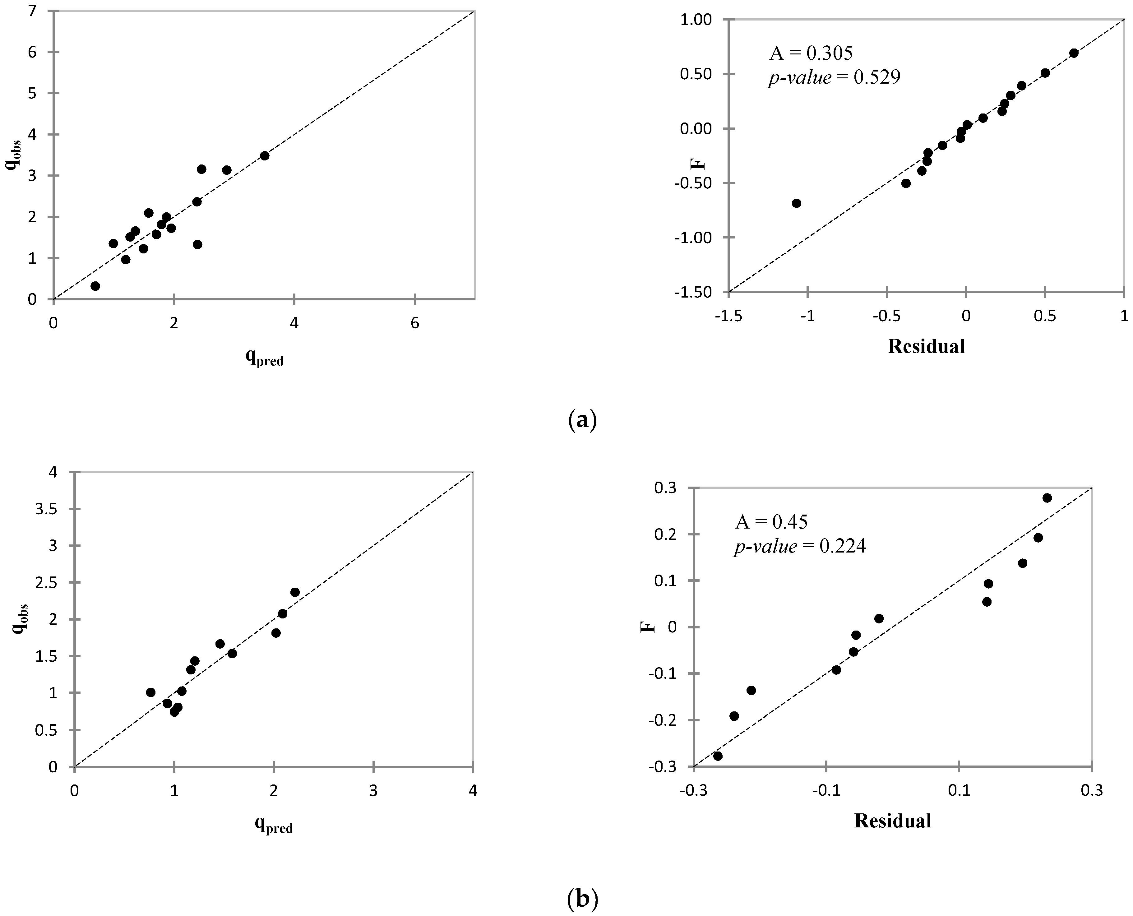
The resulting regression models were tested for homoscedasticity and normality of the residuals. White’s test showed that the residuals were homoscedastic. Based on the Anderson–Darling test (the value of test A is given in Figure 6) and the Shapiro–Wilk test, the residuals were found to have a normal distribution.
4. Conclusions
In the paper, values of the seasonality ratio (SR), cyclic seasonality index (SI) and seasonality histograms (SHs) were determined for regionalization of low flow characteristics in the catchments located on the area of the Upper Vistula basin. The predictive low flow models developed in the study area can be used for the low flow estimation in ungauged catchments. They provide information on the seasonality of low flow occurrence with varying accuracy. The most accurate information was obtained from seasonality histograms (SH), SI being a compact indicator and SR is a simplified indicator. For all analyzed indices, the occurrence of winter low flow seasonality concerned the same four catchments. In contrast, summer low flows occurred in the remaining 28 catchments. However, a more detailed histogram analysis made it possible to identify catchments of mixed type (nine catchments). In their case, despite dominant summer low flows, winter low flows were also observed.
Basing on determined seasonality indices of analyzed catchments of the upper Vistula river basin, regional regression models for low flow q95 were determined. The regression relations for the global model (without clustering) and for two groups (winter and summer low flow seasonality) were based on catchment slope, which had a positive designation. For the three groups, the factor influencing q95 was soils (cambisols), which had a positive designation in the case of summer low flow seasonality and a negative designation in the case of the mixed group. This is related to the location of the catchment in the Upper Vistula river basin. The mixed group includes catchments located in upland, Carpathian foothills and mountain climates. In terms of water circulation, the catchments of this group are characterized by poorly permeable and impermeable soils. On the other hand, catchments characterized by summer low flow seasonality are located in upland climate and sub-Carpathians and are characterized by occurrence of moderately and easily permeable soils.
The procedure is one of the proposals for determining low flow, based on the seasonality of its occurrence, which should be supplemented in the future with a larger number of catchments and other methods for their classification. The results indicate that the determination of regression models for different groups of low flow seasonality may be a promising tool for the determination of this parameter in ungauged catchments. The results of the predictive regression models can be used to calculate low flows in ungauged catchments for various water management purposes. The results of such studies are particularly important for the design of new facilities and the modernization of existing water intakes for small local water supply systems. Climate change is causing the current local water intakes to be insufficient for the growing needs of the population in Poland and other countries. Information on streamflow patterns throughout the river network are needed to provide useful information to all concerned, which can then be used to propose regulations that are consistent with the hydrological patterns of each catchment. The analysis of the seasonality of low flows can provide water management information by revealing when low flows are likely to occur and by providing context for predicting the regionally varying impacts of climate change on low flows.
Author Contributions
Conceptualization, A.C.; methodology, A.C.; software, G.K.; validation, A.C. and G.K.; investigation, A.C. and G.K.; writing—original draft preparation, A.C. and G.K.; writing—review and editing, A.C. and G.K.; visualization, A.C. and G.K.; supervision A.C. and G.K. All authors have read and agreed to the published version of the manuscript.
Funding
This research received no external funding.
Data Availability Statement
Not applicable.
Conflicts of Interest
The authors declare no conflict of interest.
References
- Tallaksen, L.M.; van Lanen, H. Hydrological Drought: Processes and Estimation Methods for Streamflow and Groundwater; Elsevier Science: Amsterdam, The Netherlands, 2004. [Google Scholar]
- Laaha, G.; Blöschl, G. A national low flow estimation procedure for Austria. Hydrol. Sci. J. 2007, 52, 625–644. [Google Scholar] [CrossRef] [Green Version]
- Banasik, K.; Kaznowska, E.; Letkiewicz, B.; Wasilewicz, M. Analysis of selected hydrological characteristics of two small lowland catchments. Acta Sci. Polonorum. Form. Circumiectus 2022, 21, 33. [Google Scholar] [CrossRef]
- Gustard, A.; Young, A.; Rees, G.; Holmes, M. Operational hydrology. In Hydrological Drought. Processes and Estimation Methods for Streamflow and Groundwater; Tallaksen, L., van Lanen, H.A.J., Eds.; Elsevier: Amsterdam, The Netherlands, 2004; pp. 455–498. [Google Scholar]
- Jungwirth, M.; Haidvogl, G.; Moog, O.; Muhar, S.; Schmutz, S. Angewandte Fischökologie an Fließgewässern; Facultas Universitätsverlag: Wien, Austria, 2003. [Google Scholar]
- Kozek, M.; Tomaszewski, E. Selected Characteristics of Hydrological Drought Progression in the Upper Warta River Catchment. Acta Sci. Pol. Formatio Circumiectus 2018, 17, 77–87. [Google Scholar] [CrossRef]
- Brunner, M.I.; Tallaksen, L.M. Proneness of European Catchments to Multiyear Streamflow Droughts. Water Resour. Res. 2019, 55, 8881–8894. [Google Scholar] [CrossRef] [Green Version]
- Floriancic, M.G.; Berghuijs, W.R.; Molnar, P.; Kirchner, J.W. Seasonality and Drivers of Low Flows across Europe and the United States. Water Resour. Res. 2021, 57, e2019WR026928. [Google Scholar] [CrossRef]
- Smakhtin, V.U. Low flow hydrology: A review. J. Hydrol. 2001, 240, 147–186. [Google Scholar] [CrossRef]
- Młyński, D.; Wałęga, A.; Bugajski, P.; Operacz, A.; Kurek, K. Verification of empirical formulas for calculating mean low flow with the view to evaluating available water resources. Acta Sci. Pol. Formatio Circumiectus 2019, 18, 83–92. [Google Scholar] [CrossRef]
- Dierauer, J.R.; Whitfield, P.H.; Allen, D.M. Climate Controls on Runoff and Low Flows in Mountain Catchments of Western North America. Water Resour. Res. 2018, 54, 7495–7510. [Google Scholar] [CrossRef]
- Vezza, P.; Comoglio, C.; Rosso, M.; Viglione, A. Low Flows Regionalization in North-Western Italy. Water Resour. Manag. 2010, 24, 4049–4074. [Google Scholar] [CrossRef]
- De Serrano, L.O.; Ribeiro, R.B.; Borges, A.C.; Pruski, F.F. Low-Flow Seasonality and Effects on Water Availability throughout the River Network. Water Resour. Manag. 2020, 34, 1289–1304. [Google Scholar] [CrossRef]
- Jokiel, P. O sezonowym rozmieszczeniu odpływu w wybranych rzekach środkowej Polski. Wiad. Met. Hydrol. Gosp. Wod. 2009, 3, 15–29. (In Polish) [Google Scholar]
- Jokiel, P.; Stanisławczyk, B. Zmiany i wieloletnia zmienność sezonowości przepływu wybranych rzek Polski. Czas. Geogr. 2016, 144, 9–33. (In Polish) [Google Scholar] [CrossRef]
- Demirel, M.C.; Booij, M.J.; Hoekstra, A.Y. Impacts of climate change on the seasonality of low flows in 134 catchments in the River Rhine basin using an ensemble of bias-corrected regional climate simulations. Hydrol. Earth Syst. Sci. 2013, 17, 4241–4257. [Google Scholar] [CrossRef] [Green Version]
- Vlach, V.; Ledvinka, O.; Matouskova, M. Changing Low Flow and Streamflow Drought Seasonality in Central European Headwaters. Water 2020, 12, 3575. [Google Scholar] [CrossRef]
- Laaha, G. A mixed distribution approach for low-flow frequency analysis–Part 1: Concept, performance and effect of seasonality. Hydrol. Earth Syst. Sci. Discuss. 2022, pp. 1–19, Preprint. Available online: https://hess.copernicus.org/preprints/hess-2022-195/hess-2022-195.pdf (accessed on 30 November 2022). [CrossRef]
- Schreiber, P.; DeMuth, S. Regionalization of low flows in southwest Germany. Hydrol. Sci. J. 1997, 42, 845–858. [Google Scholar] [CrossRef] [Green Version]
- Aschwanden, H.; Kan, C. Le d´ebit d’´etiage Q347—Etat de la question. In Communications Hydrologiques; Service Hydrologique et G´eologique National: Berne, Switzerland, 1999; Volume 27. [Google Scholar]
- Pournasiri Poshtiri, M.; Pal, I.; Lall, U.; Naveau, P.; Towler, E. Variability patterns of the annual frequency and timing of low streamflow days across the United States and their linkage to regional and large-scale climate. Hydrol. Process. 2019, 33, 1569–1578. [Google Scholar] [CrossRef]
- Dingman, S.L.; Lawlor, S.C. Estimating low-flow quantiles from drainage-basin characteristics in new hampshire and vermont. JAWRA J. Am. Water Resour. Assoc. 1995, 31, 243–256. [Google Scholar] [CrossRef]
- Fangmann, A.; Haberlandt, U. Statistical approaches for identification of low-flow drivers: Temporal aspects. Hydrol. Earth Syst. Sci. 2019, 23, 447–463. [Google Scholar] [CrossRef] [Green Version]
- Laaha, G. Process Based Regionalisation of Low Flows. Ph.D. Dissertation, Institut für Konstruktiven Wasserbau, Wien, Austria, 2006. [Google Scholar]
- Laaha, G.; Blöschl, G. A comparison of low flow regionalisation methods—Catchment grouping. J. Hydrol. 2006, 323, 193–214. [Google Scholar] [CrossRef]
- Laaha, G.; Blöschl, G. Seasonality indices for regionalizing low flows. Hydrol. Process. 2006, 20, 3851–3878. [Google Scholar] [CrossRef]
- Rotnicka, J. Teoretyczne Podstawy Wydzielania Okresów Hydrologicznych i Analizy Reżimu Rzecznego na Przykładzie Rzeki Prosny; Prace Komisji Geograficzno-Geologicznej PTPN; Państwowe Wydawn: Naukowe, Poland, 1977; Volume XVIII. [Google Scholar]
- Jokiel, P.; Tomalski, P. Próba wyznaczenia sezonów hydrologicznych w obrębie rocznych hydrogramów przepływu wybranych rzek środkowej Polski. Monografie. Red. A. Magnuszewski. Polska Akademia Nauk 2014, 20, 203–217. (In Polish) [Google Scholar]
- Cupak, A. Regionalization methods for low flow estimation in ungauged catchments–a review. Acta Sci. Pol. Circumiectus 2020, 19, 21–35. [Google Scholar] [CrossRef]
- Kondracki, J. Geografia Regionalna Polski; PWN: Warszawa, Poland, 2000. [Google Scholar]
- Dobrzański, B.; Witek, T.; Kowaliński, S.; Królikowski, L.; Kuźnicki, F.; Siuta, J.; Skawina, T.; Strzemski, M.; Trzuskowska, R.; Uggla, H.; et al. Polska Mapa Gleb; Wydawnictwo Geologiczne: Warszawa, Poland, 1972. [Google Scholar]
- GIOŚ. Corine Land Cover. 2022. Available online: http://clc.gios.gov.pl (accessed on 1 December 2022).
- Chełmicki, W. Location, division and features of the basin. In Upper Vistula Basin; Dynowska, I., Maciejewski, M., Eds.; PWN: Kraków, Poland, 1991. [Google Scholar]
- Więcławik, S. Geology. In Upper Vistula Basin; Dynowska, I., Maciejewski, M., Eds.; PWN: Kraków, Poland, 1991. [Google Scholar]
- Burn, D.H. Regionalisation of catchments for regional flood frequency analysis. J. Hydrol. Eng. 1997, 2, 6–82. [Google Scholar] [CrossRef]
- Young, A.R.; Round, C.E.; Gustard, A. Spatial and temporal variations in the occurrence of low flow events in the UK. Hydrol. Earth Syst. Sci. 2000, 4, 35–45. [Google Scholar] [CrossRef] [Green Version]
- Burn, D.H. Evaluation of regional flood frequency analysis with a region of influence approach. Water Resour. Res. 1990, 26, 2257–2265. [Google Scholar] [CrossRef]
- Wang, W.; Lu, Y. Analysis of the Mean Absolute Error (MAE) and the Root Mean Square Error (RMSE) in Assessing Rounding Model. In IOP Conference Series: Materials, Science and Engineering; IOP Publishing: Bristol, UK, 2018; Volume 324. [Google Scholar] [CrossRef]
- Raczyński, K.; Dyer, J. Multi-annual and seasonal variability of low-flow river conditions in southeastern Poland. Hydrol. Sci. J. 2020, 65, 2561–2576. [Google Scholar] [CrossRef]
- Guilford, J.P. Fundamental Statistics in Psychology and Education; McGraw-Hill: New York, NY, USA, 1965. [Google Scholar]
- Kohnová, S.; Hlavcova, K.; Szolgay, J.; Stevkova, A. Seasonality analysis of the occurrence of low flows in Slovakia. In Proceedings of the International Symposium on Water Management and Hydraulic Engineering, Ohrid, Macedonia, 1–5 September 2009; pp. 711–719. [Google Scholar]
Figure 1.
The location of the Upper Vistula river basin and analyzed catchments (points show the location of the catchment areas selected for the analysis).
Figure 1.
The location of the Upper Vistula river basin and analyzed catchments (points show the location of the catchment areas selected for the analysis).

Figure 2.
Specific low flow discharge q95 for analyzed catchments of the Upper Vistula basin, where: 1—Dłubnia; 2—Opatówka; 3—Biała Tarnowska; 4—Szreniawa; 5—Wieprzówka; 6—Łeg; 7—Tanew; 8—Biała; 9—Pszczynka; 10—Skawa; 11—Łososinka; 12—Biała Nida; 13—Trzebośnica; 14—Czarna; 15—Soła; 16—Wisła; 17—Dunajec; 18—Koprzywianka; 19—Skawica; 20—Czarna Nida; 21—Wschodnia; 22—Ropa; 23—Jasiołka; 24—Solinka; 25—Osława; 26—Stupnica; 27—Mleczka; 28—Łubinka; 29—Grabinianka; 30—Wielkopolka; 31—Wisłoka; 32—Breń.

Figure 3.
Seasonality ratio (SR) for summer and winter low flow discharge for analyzed catchments.

Figure 4.
Map of SI (a) and seasonality histograms (b) for analyzed catchments; the x-axis is in the hydrological year for analyzed catchments and y-axis in all cases is from 0 to 400.
Figure 4.
Map of SI (a) and seasonality histograms (b) for analyzed catchments; the x-axis is in the hydrological year for analyzed catchments and y-axis in all cases is from 0 to 400.

Figure 5.
Localization of catchments for three type of seasonality.

Figure 6.
Differences between observed and calculated q95 (dm3∙s−1∙km−2) for (a) cluster 3_2 and (b) cluster 3_3.
Figure 6.
Differences between observed and calculated q95 (dm3∙s−1∙km−2) for (a) cluster 3_2 and (b) cluster 3_3.


Table 1.
Statistical summary of catchments’ characteristics.
| Variable | Variable Description | Units | Min. | Mean | Max. |
|---|---|---|---|---|---|
| A | Catchment area | km2 | 66.3 | 475.73 | 2034.0 |
| L | Length of the watercourse | km | 8.8 | 34.33 | 72.0 |
| P | Mean annual precipitation | mm | 574 | 729.28 | 1033 |
| I | Mean catchment slope | - | 0.002 | 0.021 | 0.091 |
| Hme | Mean catchment altitude | m a.s.l. | 191.00 | 388.86 | 836.00 |
| LU4 | Forests | % | 3.00 | 31.29 | 67.60 |
| LU3 | Grassland | % | 0.00 | 8.29 | 32.00 |
| LU2 | Arable land | % | 7.40 | 47.61 | 86.00 |
| LU1 | Built-up area | % | 0.00 | 6.55 | 29.88 |
| S1 | Fluvisols | % | 0.00 | 15.93 | 28.20 |
| S2 | Cambisols | % | 0.00 | 54.48 | 100.00 |
| S3 | Arenosols | % | 0.00 | 10.34 | 65.00 |
Table 2.
Regional regression model based on K-mean method.
| Group | Number of Catchments | Type of Seasonality | Model | R2 | R2adj | R2cv | RMSE | RMSEcv |
|---|---|---|---|---|---|---|---|---|
| global | 32 | - | q95 = 1.24 + 27.08∙I | 41 | 39 | 23 | 0.71 | 0.81 |
| Two clusters | ||||||||
| 2_1 | 23 | summer | q95 = 1.86 + 20.31∙I − 0.042∙S1 | 52 | 47 | 30 | 0.56 | 0.74 |
| 2_2 | 9 | winter | q95 = 3.61 + 25.64∙I − 0.041∙LU2 | 88 | 84 | 49 | 0.44 | 0.66 |
| Three clusters | ||||||||
| 3_2 | 16 | mixed | q95 = 0.92−0.02∙S2−0.02∙LU5 + 0.007∙Hme | 76 | 70 | 67 | 0.46 | 0.49 |
| 3_3 | 12 | summer | q95 = −2.66 + 0.009∙S2 + 0.03∙LU5 + 0.004∙P | 88 | 83 | 66 | 0.21 | 0.36 |
Disclaimer/Publisher’s Note: The statements, opinions and data contained in all publications are solely those of the individual author(s) and contributor(s) and not of MDPI and/or the editor(s). MDPI and/or the editor(s) disclaim responsibility for any injury to people or property resulting from any ideas, methods, instructions or products referred to in the content. |
© 2023 by the authors. Licensee MDPI, Basel, Switzerland. This article is an open access article distributed under the terms and conditions of the Creative Commons Attribution (CC BY) license (https://creativecommons.org/licenses/by/4.0/).
Share and Cite
MDPI and ACS Style
Cupak, A.; Kaczor, G. Determination of Seasonal Indices for the Regionalization of Low Flows in the Upper Vistula River Basin. Water 2023, 15, 246. https://doi.org/10.3390/w15020246
AMA Style
Cupak A, Kaczor G. Determination of Seasonal Indices for the Regionalization of Low Flows in the Upper Vistula River Basin. Water. 2023; 15(2):246. https://doi.org/10.3390/w15020246
Chicago/Turabian StyleCupak, Agnieszka, and Grzegorz Kaczor. 2023. "Determination of Seasonal Indices for the Regionalization of Low Flows in the Upper Vistula River Basin" Water 15, no. 2: 246. https://doi.org/10.3390/w15020246
Note that from the first issue of 2016, this journal uses article numbers instead of page numbers. See further details here.