
Brazilian Annual Precipitation Analysis Simulated by the Brazilian Atmospheric Global Model

 , , , ,
Abstract
:1. Introduction
2. Materials and Methods
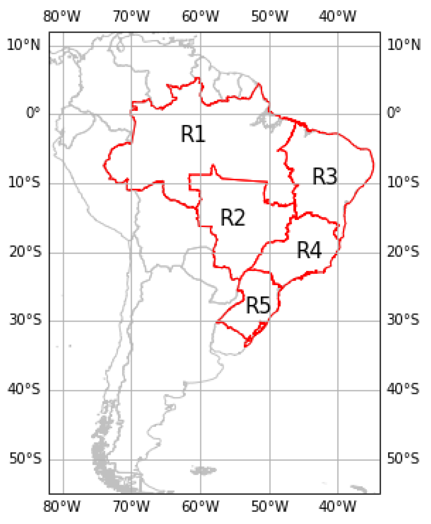
2.1. Study Area
2.2. General Circulation Model and Climate Data
2.3. Data Analysis
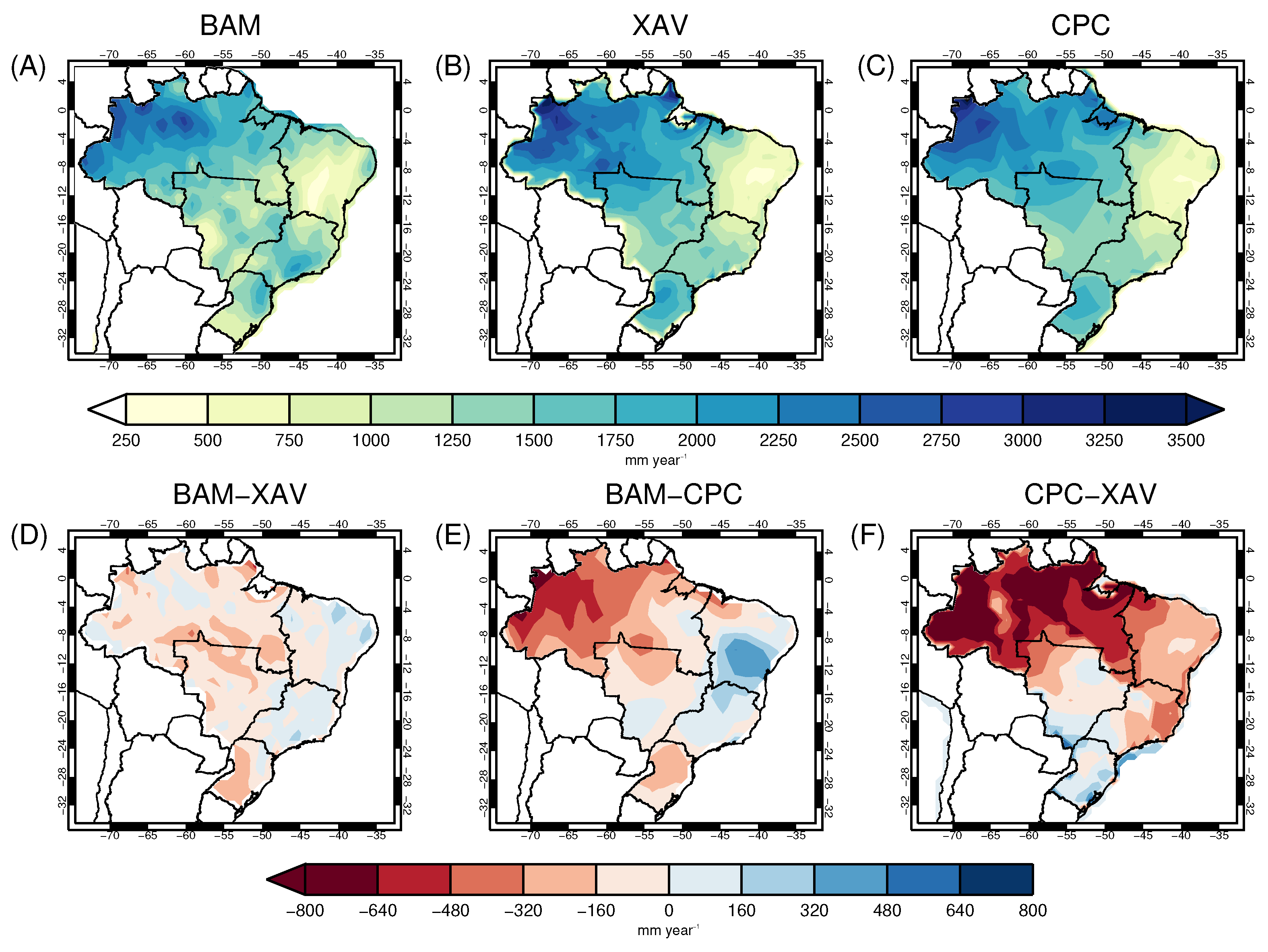
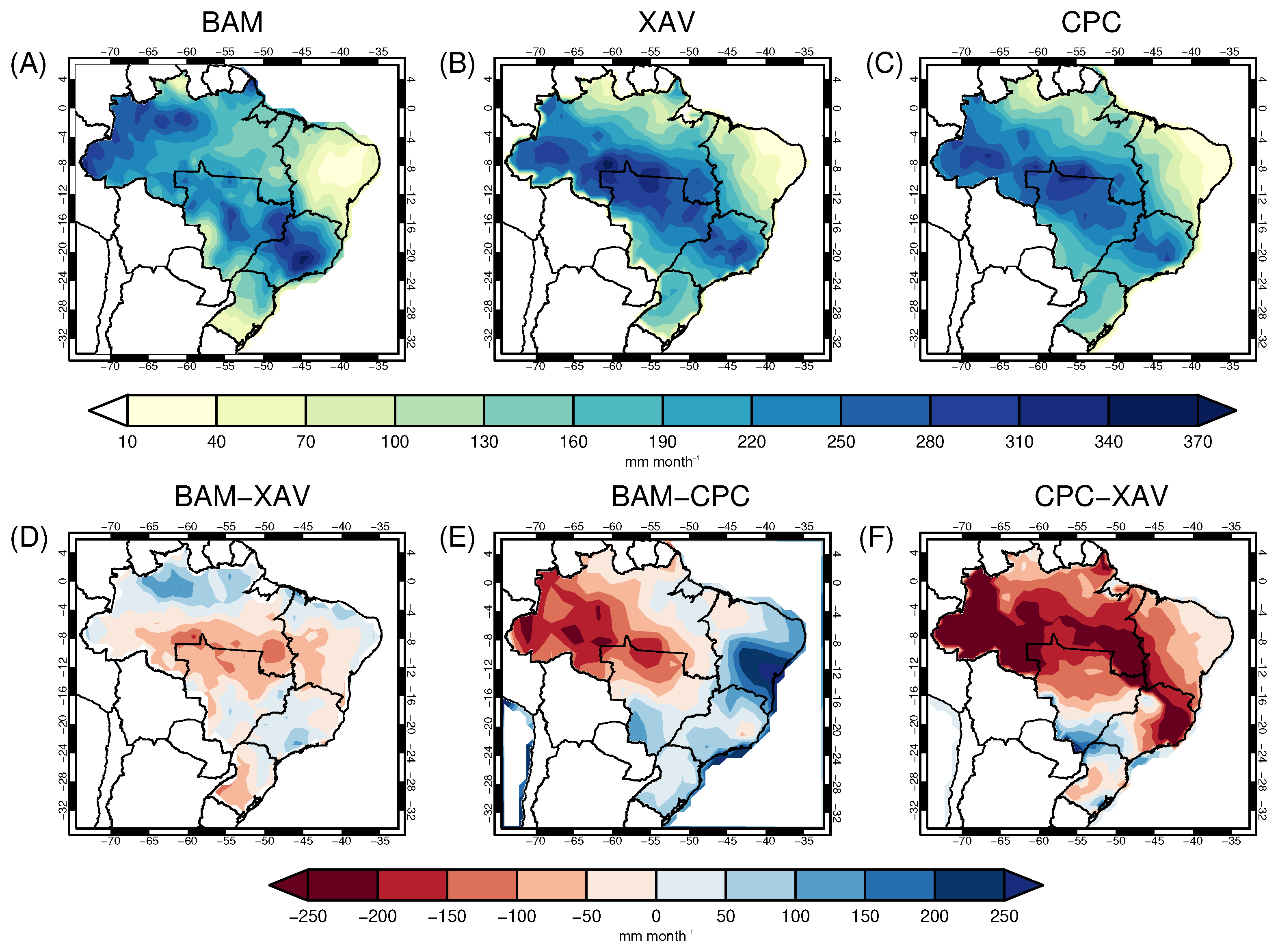
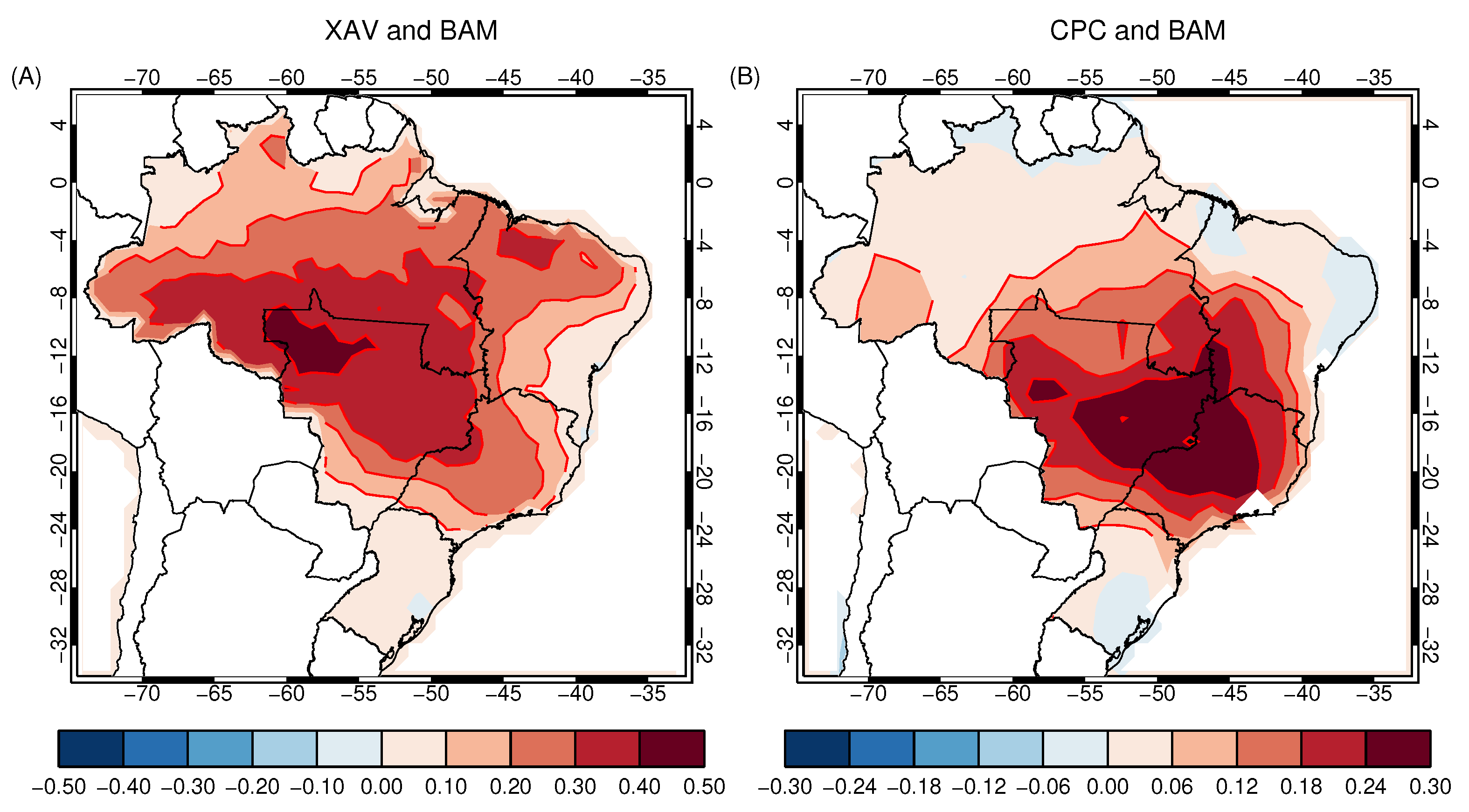
3. Results
4. Discussion
5. Conclusions
Supplementary Materials
Author Contributions
Funding
Data Availability Statement
Acknowledgments
Conflicts of Interest
Abbreviations
| AMIP | Atmospheric Model Intercomparison Project |
| BAM | Brazilian Atmospheric Model |
| CPTEC | Center for Weather Forecasting and Climate Studies |
| INPE | National Institute for Space Research |
| CPC | Climate Prediction Center |
| SACZ | South Atlantic Convergence Zone |
| BR | Brazil |
| SA | South America |
| SAMA | South American Monsoon System |
| ITCZ | Intertropical Convergence Zone |
| SST | Sea surface temperature |
| BESM | Brazilian Earth System Model |
| IBGM | Brazilian Institute of Geography and Statistics |
| AGCM | Atmospheric General Circulation Models |
| COLA | Center for Ocean–Earth–Atmosphere Studies |
| NCEP | National Centers for Environmental Prediction |
| NOAA | National Oceanic and Atmospheric Administration |
References
- Tomaziello, A.C.N. Influências da Temperatura da Superfície do mar e da Umidade do solo na Precipitação Associada à Zona de Convergência do Atlântico Sul. Ph.D. Thesis, Universidade de São Paulo, São Paulo, Brazil, 2010. [Google Scholar]
- Marengo, J.A.; Torres, R.R.; Alves, L.M. Drought in Northeast Brazil—Past, present, and future. Theor. Appl. Climatol. 2017, 129, 1189–1200. [Google Scholar] [CrossRef]
- Rocha, F.; Silva, W.; Ribeiro, B. Synoptic Analysis of a Period with Above-normal Precipitation during the Dry Season in Southeastern Brazil. Adv. Res. 2019, 19, 1–13. [Google Scholar] [CrossRef]
- Silva Dias, M.A.F.; Silva, M.G.A.J. Para entender tempo e clima. In Tempo e Clima no Brasil; Cavalcanti, I.F.A., Ferreira, N.J., Justi Da Silva, M.G.A., Silva Dias, M.A.F., Eds.; Oficina de Textos: São Paulo, Brazil, 2009; Volume 1, pp. 15–21, 135–147. [Google Scholar]
- Grimm, A.M. Interannual climate variability in South America: Impacts on seasonal precipitation, extreme events, and possible effects of climate change. Stoch. Environ. Res. Risk Assess. 2011, 25, 537–554. [Google Scholar] [CrossRef]
- Ferreira, G.W.S.; Reboita, M.S. A New Look into the South America Precipitation Regimes: Observation and Forecast. Atmosphere 2022, 13, 873. [Google Scholar] [CrossRef]
- Reboita, M.S.; Gan, M.A.; Rocha, R.P.; Ambrizzi, T. Precipitation regimes in South America: A literature review. Rev. Bras. Meteorol. 2010, 25, 185–204. [Google Scholar] [CrossRef]
- Gan, M.; Kousky, V.; Ropelewski, C. The south america monsoon circulation and its relationship to rainfall over west-central brazil. J. Clim. 2004, 17, 47–66. [Google Scholar] [CrossRef]
- Marengo, J.A.; Liebmann, B.; Grimm, A.M.; Misra, V.; Silva Dias, P.L.; Cavalcanti, I.F.A.; Carvalho, L.M.V.; Berbery, E.H.; Ambrizzi, T.; Vera, C.S.; et al. Recent developments on the South American monsoon system. Int. J. Climatol. 2012, 32, 1–21. [Google Scholar] [CrossRef] [Green Version]
- Wang, B.; Biasutti, M.; Byrne, M.P.; Castro, C.; Chang, C.; Cook, K.; Fu, R.; Grimm, A.M.; Ha, K.; Hendon, H.; et al. Monsoons Climate Change Assessment. Bull. Am. Meteorol. Soc. 2020, 102, E1–E19. [Google Scholar] [CrossRef]
- Gan, M.; Santos, L.F.; Lima, J.; Afonso, J.; Silva, A. Monção da América do Sul. Chapter 2009, 19, 297–312. [Google Scholar]
- Kodama, Y. Large-scale common features of subtropical precipitation zones (the baiu frontal zone, the spcz, and the sacz) part i: Characteristics of subtropical frontal zones. J. Meteorol. Soc. Jpn. Ser. II 1992, 70, 813–836. [Google Scholar] [CrossRef] [Green Version]
- Kodama, Y. Large-scale common features of sub-tropical convergence zones (the baiu frontal zone, the spcz, and the sacz) part ii: Conditions of the circulations for generating the stczs. J. Meteorol. Soc. Jpn. Ser. II 1993, 71, 581–610. [Google Scholar] [CrossRef]
- Carvalho, L.M.V.; Jones, C.; Liebmann, B. Extreme precipitation events in southeastern South America and large-scale convective patterns in the South Atlantic Convergence Zone. J. Clim. 2002, 17, 2377–2394. [Google Scholar] [CrossRef]
- Quadro, M.F.L.; Dias, M.A.F.S.; Herdies, D.L.; Gonçalves, L.G.G. Climatological analysis of precipitation and moisture transport in the SACZ region through the new generation of reanalyses. Rev. Bras. Meteorol. 2012, 27, 152–162. [Google Scholar] [CrossRef] [Green Version]
- Marengo, J.A.; Nobre, C.A.; Seluchi, M.E.; Cuartas, A.; Alves, L.M.; Mendiondo, E.M.; Obregon, G.; Sampaio, G. The drought and water crisis of 2014–2015 in são paulo. Rev. USP 2015, 106, 31–44. Available online: http://www.revistas.usp.br/revusp/article/view/110101 (accessed on 10 February 2020). [CrossRef] [Green Version]
- Cavalcanti, I.F.A.; Marengo, J.A.; Satyamurty, P.; Nobre, C.A.; Trosnikov, I.; Bonatti, J.P.; Manzi, A.O.; Tarasova, T.; Pezzi, L.P.; D’Almeida, C.; et al. Global Climatological Features in a Simulation Using the CPTEC–COLA AGCM. J. Clim. 2002, 15, 2965–2988. [Google Scholar] [CrossRef]
- Marengo, J.A.; Cavalcanti, I.F.A.; Satyamurty, P.; Trosnikov, I.; Nobre, C.A.; Bonatti, J.P.; Camargo, H.; Sampaio, G.; Sanches, M.B.; Manzi, A.O.; et al. Assessment of regional seasonal rainfall predictability using the CPTEC/COLA atmospheric GCM. Clim. Dyn. 2003, 21, 459–475. [Google Scholar] [CrossRef]
- Coelho, C.A.; de Souza, D.C.; Kubota, P.Y.; Costa, S.; Menezes, L.; Guimaraes, B.S.; Figueroa, S.N.; Bonatti, J.P.; Cavalcanti, I.F.; Sampaio, G.; et al. Evaluation of climate simulations produced with the Brazilian global atmospheric model version 1.2. Clim. Dyn. 2021, 56, 873–898. [Google Scholar] [CrossRef]
- Nobre, P.; Siqueira, L.; Almeida, R.; Malagutti, M.; Giarolla, E.; Hammes, G.O.P.; Bottino, M.; Kubota, P.; Figueroa, S.; Costa, M.; et al. Climate Simulation and Change in the Brazilian Climate Model. J. Clim. 2013, 26, 6716–6732. [Google Scholar] [CrossRef]
- Figueroa, S.N.; Bonatti, J.P.; Kubota, P.Y.; Grell, G.A.; Morrison, H.; Barros, S.R.M.; Fernandez, J.P.R.; Ramirez, E.; Siqueira, L.; Luzia, G.; et al. The Brazilian Global Atmospheric Model (BAM): Performance for Tropical Rainfall Forecasting and Sensitivity to Convective Scheme and Horizontal Resolution. Weather. Forecast. 2016, 31, 1547–1572. [Google Scholar] [CrossRef]
- Cavalcanti, I.F.A.; Raia, A. Lifecycle of South American Monsoon System simulated by CPTEC/INPE AGCM. Int. J. Climatol. 2017, 37, 878–896. [Google Scholar] [CrossRef]
- Souza, D.C.; Kubota, P.Y.; Figueroa, S.N.; Gutierrez, E.M.A.R.; Coelho, C.A.S. Impacto da Resolução Horizontal na Simulação dos Jatos de Baixos Níveis na América do Sul usando o Modelo Global do CPTEC. In Estudos Interdisciplinares nas Ciências Exatas e da Terra e Engenharias 4, 82nd ed.; Atena Editora: Ponta Grossa, Brazil, 2019; pp. 205–217. [Google Scholar] [CrossRef]
- Cavalcanti, I.F.A.; Silveira, V.P.; Figueroa, S.N.; Kubota, P.Y.; Bonatti, J.P.; de Souza, D.C. Climate variability over South America-regional and large scale features simulated by the Brazilian Atmospheric Model (BAM-v0). Int. J. Climatol. 2020, 40, 2845–2869. [Google Scholar] [CrossRef]
- Guimarães, B.S.; Coelho, C.A.; Woolnough, S.J.; Kubota, P.Y.; Bastarz, C.F.; Figueroa, S.N.; Bonatti, J.P.; de Souza, D.C. Configuration and hindcast quality assessment of a Brazilian global sub-seasonal prediction system. Q. J. R. Meteorol. Soc. 2020, 146, 1067–1084. [Google Scholar] [CrossRef]
- Guimarães, B.D.S.; Coelho, C.A.D.S.; Woolnough, S.J.; Kubota, P.Y.; Bastarz, C.F.; Figueroa, S.N.; Bonatti, J.P.; de Souza, D.C. An inter-comparison performance assessment of a Brazilian global sub-seasonal prediction model against four sub-seasonal to seasonal (S2S) prediction project models. Clim. Dyn. 2021, 56, 2359–2375. [Google Scholar] [CrossRef]
- Baker, J.C.A.; de Souza, D.C.; Kubota, P.Y.; Buermann, W.; Coelho, C.A.S.; Andrews, M.B.; Gloor, M.; Garcia-Carreras, L.; Figueroa, S.N.; Spracklen, D.V. An Assessment of Land–Atmosphere Interactions over South America Using Satellites, Reanalysis, and Two Global Climate Models. J. Hydrometeorol. 2021, 22, 905–922. [Google Scholar] [CrossRef]
- Lima, I.T. O Início da Estação Chuvosa na América do Sul e Processos Atmosféricos e de Superfície Associados. Master’s Thesis, Instituto Nacional de Pesquisas Espaciais (INPE), São José dos Campos, Brazil, 2021; 177p. Available online: http://urlib.net/rep/8JMKD3MGP3W34R/44478D2 (accessed on 10 February 2020).
- Coelho, C.A.; de Souza, D.C.; Kubota, P.Y.; Cavalcanti, I.F.; Baker, J.C.; Figueroa, S.N.; Firpo, M.A.; Guimaraes, B.S.; Costa, S.M.; Goncalves, L.J.; et al. Assessing the representation of South American monsoon features in Brazil and U.K. climate model simulations. Clim. Resil. Sustain. 2022, 1, e27. [Google Scholar] [CrossRef]
- Han, J.; Pan, H.-L. Revision of Convection and Vertical Diffusion Schemes in the NCEP Global Forecast System. Weather. Forecast. 2011, 26, 520–533. [Google Scholar] [CrossRef]
- Tiedtke, M. The sensitivity of the time-mean large-scale flow to cumulus convection in the ECMWF model. In Proceedings of the Workshop on Convection in Large-Scale Models, ECMWF, Reading, UK, 4–8 December 1989; pp. 297–316. [Google Scholar]
- Morrison, G.; Curry, J.A.; Khvorostyanov, V.I. A new double-moment microphysics parameterization for application in cloud and climate models. Part I Descr. J. Atmos. Sci. 2005, 62, 1665–1677. [Google Scholar] [CrossRef]
- Kubota, P.Y. Variabilidade da Energia Armazenada na Superfície e o seu Impacto na Definição do Padrão de Precipitação na América do Sul. Ph.D. Thesis, Instituto Nacional de Pesquisas Espaciais (INPE), São José dos Campos, Brazil, 2012. Available online: http://urlib.net/8JMKD3MGP7W/3CCP5R2 (accessed on 15 March 2021).
- Tarasova, T.; Figueroa, S.; Barbosa, H. Incorporation of New Solar Radiation Scheme into CPTEC GCM; Instituto Nacional de Pesquisas Espaciais: São José dos Campos, Brazil, 2007. [Google Scholar]
- Holtslag, A.A.M.; Boville, B.A. Local versus nonlocal boundary-layer diffusion in a global climate model. J. Clim. 1992, 6, 1825–1842. [Google Scholar] [CrossRef]
- Berrisford, P.; Dee, D.; Poli, P.; Brugge, R.; Fielding, K.; Fuentes, M.; Simmons, A. The ERA-Interim Archive Version 2.0; ERA Report Series 1; ECMWF: Reading, UK; Bershire, UK, 2011. [Google Scholar]
- Smith, T.M.; Reynolds, R.W.; Peterson, T.C.; Lawrimore, J. Improvements to NOAA’s historical merged land–ocean surface temperature analysis (1880–2006). J. Clim. 2008, 21, 2283–2296. [Google Scholar] [CrossRef]
- Xavier, A.C.; King, C.W.; Scanlon, B.R. Daily gridded meteorological variables in Brazil (1980–2013). Int. J. Clim. 2016, 36, 2644–2659. [Google Scholar] [CrossRef]
- Chen, M.; Shi, W.; Xie, P.; Silva, V.B.S.; Kousky, V.E.; Higgins, R.W.; Janowiak, J.E. Assessing objective techniques for gauge-based analyses of global daily precipitation. J. Geophys. Res. Atmos. 2008, 113, D04110. [Google Scholar] [CrossRef]
- Gandin, L.S. Objective Analysis of Meteorological Fields; Gidrometeorologicheskoe Izdatelstvo: Leningrad, Russia, 1965; 242p. [Google Scholar]
- Xie, P.; Chen, M.; Shi, W. CPC global unified gauge-based analysis of daily precipitation. In Proceedings of the 24th Conference on Hydrology, Atlanta, GA, USA, 18 January 2010; American Meteorological Society: Boston, MA, USA, 2010; Volume 2. [Google Scholar]
- Wilks, D.S. Statistical Methods in the Atmospheric Sciences, 1st ed.; Academic Press: Ithaca, NY, USA, 1995; p. 481. [Google Scholar]
- Marengo, J.A.; Nobre, C. Clima da região Amazônica. In Tempo e Clima no Brasil; Cavalcanti, I.F.A., Ferreira, N.J., Justi Da Silva, M.G.A., Silva Dias, M.A.F., Eds.; Oficina de Textos: São Paulo, Brazil, 2009; pp. 197–212. [Google Scholar]
- Grimm, A.M. Clima da Região Sul do Brasil. In Tempo e Clima no Brasil; Cavalcanti, I.F.A., Ferreira, N.J., Justi Da Silva, M.G.A., Silva Dias, M.A.F., Eds.; Oficina de Textos: São Paulo, Brazil, 2009. [Google Scholar]
- Nascimento, E. Severe storms forecast using convective parameters and mesoscale models: An operational strategy adoptable in Brazil. Rev. Bras. Meteorol. 2005, 20, 121–140. [Google Scholar]
- Cera, J.; Ferraz, S.E.T. Climate variations in precipitation in southern Brazil in present and future climate. Rev. Bras. Meteorol. 2015, 30, 81–88. [Google Scholar] [CrossRef] [Green Version]
- Britto, F.P.; Barletta, R.; Mendonça, M. Spatial and temporal variability of rainfall in Rio Grande do Sul: Influence of the El Niño Southern Oscillation phenomenon. Rev. Bras. Climatol. 2008, 3, 37–48. [Google Scholar]
- Nunes, L.; Koga, V.A.; Candido, D. Clima da região Sudeste do Brasil. In Tempo e Clima no Brasil; Cavalcanti, I.F.A., Ferreira, N.J., Justi Da Silva, M.G.A., Silva Dias, M.A.F., Eds.; Oficina de Textos: São Paulo, Brazil, 2009; Volume 1. [Google Scholar]
- Kayano, M.T.; Andreoli, R.V. Clima da região Nordeste do Brasil. In Tempo e Clima no Brasil; Cavalcanti, I.F.A., Ferreira, N.J., Justi Da Silva, M.G.A., Silva Dias, M.A.F., Eds.; Oficina de Textos: São Paulo, Brazil, 2009; Volume 1. [Google Scholar]
- Kousky, V.; Gan, M. Upper tropospheric cyclonic vortices in the tropical south atlantic. Tellus 1981, 33, 538–551. [Google Scholar] [CrossRef] [Green Version]
- Grimm, A.M.; Ferraz, S.E.T.; Gomes, J. Precipitation Anomalies in Southern Brazil Associated with El Niño and La Niña Events. J. Clim. 1998, 11, 2863–2880. [Google Scholar] [CrossRef]
- Velasco, I.; Fritsch, J.M. Mesoscale convective complexes in the Americas. J. Geophys. Res. Atmos. 1987, 92, 9591–9613. [Google Scholar] [CrossRef]
- Moura, R.; Correia, F.; Veiga, J.; Capistrano, V.; Kubota, P. Evaluation of the Brazilian Global Atmospheric Model in the Simulation of Water Balance Components in the Amazon Basin. Rev. Bras. Meteorol. 2020, 36, 23–37. [Google Scholar] [CrossRef]


| Dynamics | Eulerian (Spectral) |
| Deep Convection | Simplified Arakawa–Schubert (SAS) Convection Scheme calibrated at CPTEC [30] |
| Shallow Convection | Tieldke [31] |
| Microphysics | CliRad [32] |
| Planetary Boundary Layer | Dry-PBL [35] |
| Surface | IBIS-2.6-CPTEC [33] |
| Shortwave and Longwave Radiation | CliRad [34] |
Disclaimer/Publisher’s Note: The statements, opinions and data contained in all publications are solely those of the individual author(s) and contributor(s) and not of MDPI and/or the editor(s). MDPI and/or the editor(s) disclaim responsibility for any injury to people or property resulting from any ideas, methods, instructions or products referred to in the content. |
© 2023 by the authors. Licensee MDPI, Basel, Switzerland. This article is an open access article distributed under the terms and conditions of the Creative Commons Attribution (CC BY) license (https://creativecommons.org/licenses/by/4.0/).
Share and Cite
Bresciani, C.; Boiaski, N.T.; Ferraz, S.E.T.; Rosso, F.V.; Portalanza, D.; de Souza, D.C.; Kubota, P.Y.; Herdies, D.L. Brazilian Annual Precipitation Analysis Simulated by the Brazilian Atmospheric Global Model. Water 2023, 15, 256. https://doi.org/10.3390/w15020256
Bresciani C, Boiaski NT, Ferraz SET, Rosso FV, Portalanza D, de Souza DC, Kubota PY, Herdies DL. Brazilian Annual Precipitation Analysis Simulated by the Brazilian Atmospheric Global Model. Water. 2023; 15(2):256. https://doi.org/10.3390/w15020256
Chicago/Turabian StyleBresciani, Caroline, Nathalie Tissot Boiaski, Simone Erotildes Teleginski Ferraz, Flávia Venturini Rosso, Diego Portalanza, Dayana Castilho de Souza, Paulo Yoshio Kubota, and Dirceu Luis Herdies. 2023. "Brazilian Annual Precipitation Analysis Simulated by the Brazilian Atmospheric Global Model" Water 15, no. 2: 256. https://doi.org/10.3390/w15020256