

Deep Learning Approach with LSTM for Daily Streamflow Prediction in a Semi-Arid Area: A Case Study of Oum Er-Rbia River Basin, Morocco
 , ,
, ,  ,
,
Abstract
:1. Introduction
2. Materials and Methods
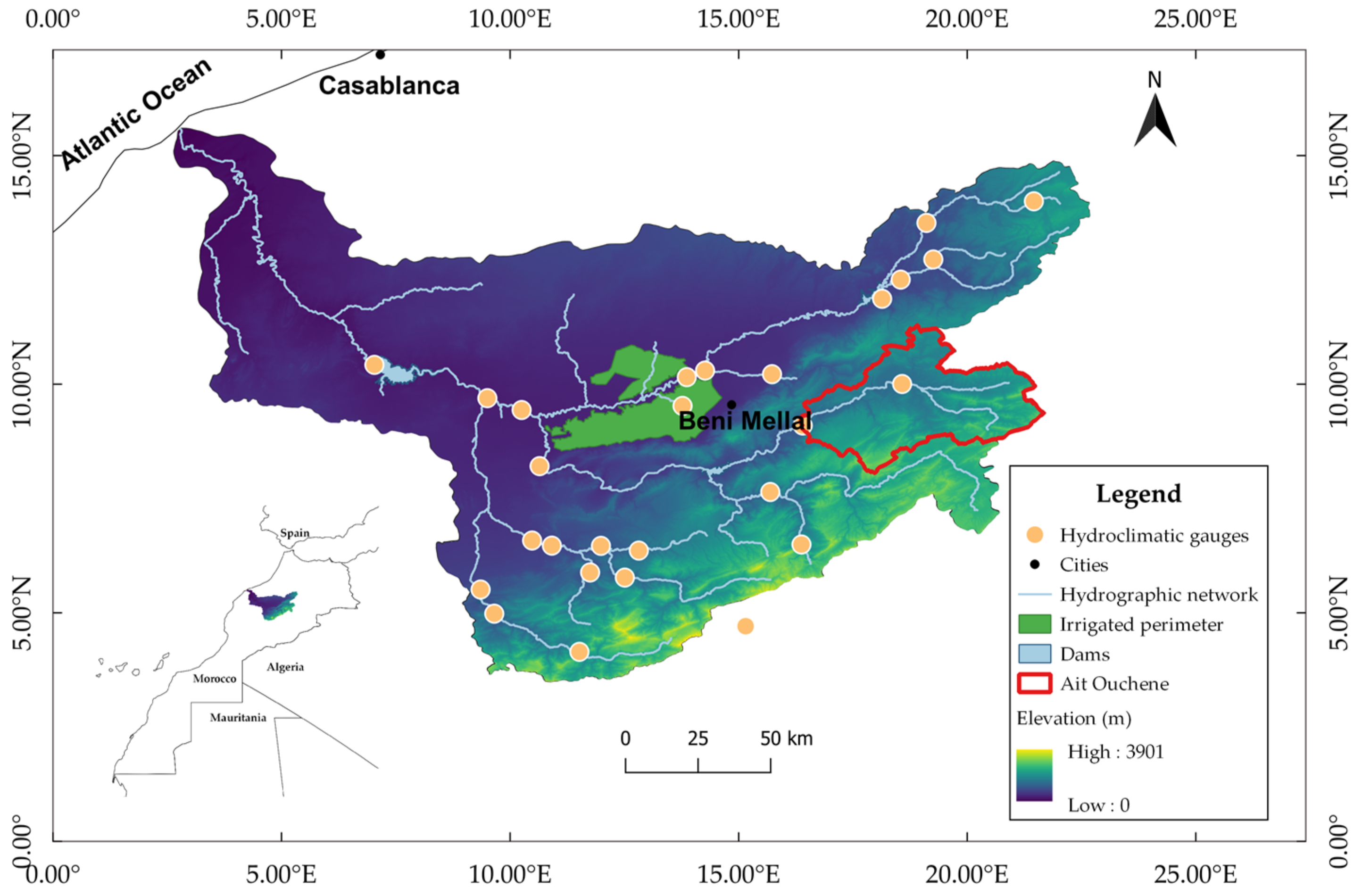
2.1. Case Study
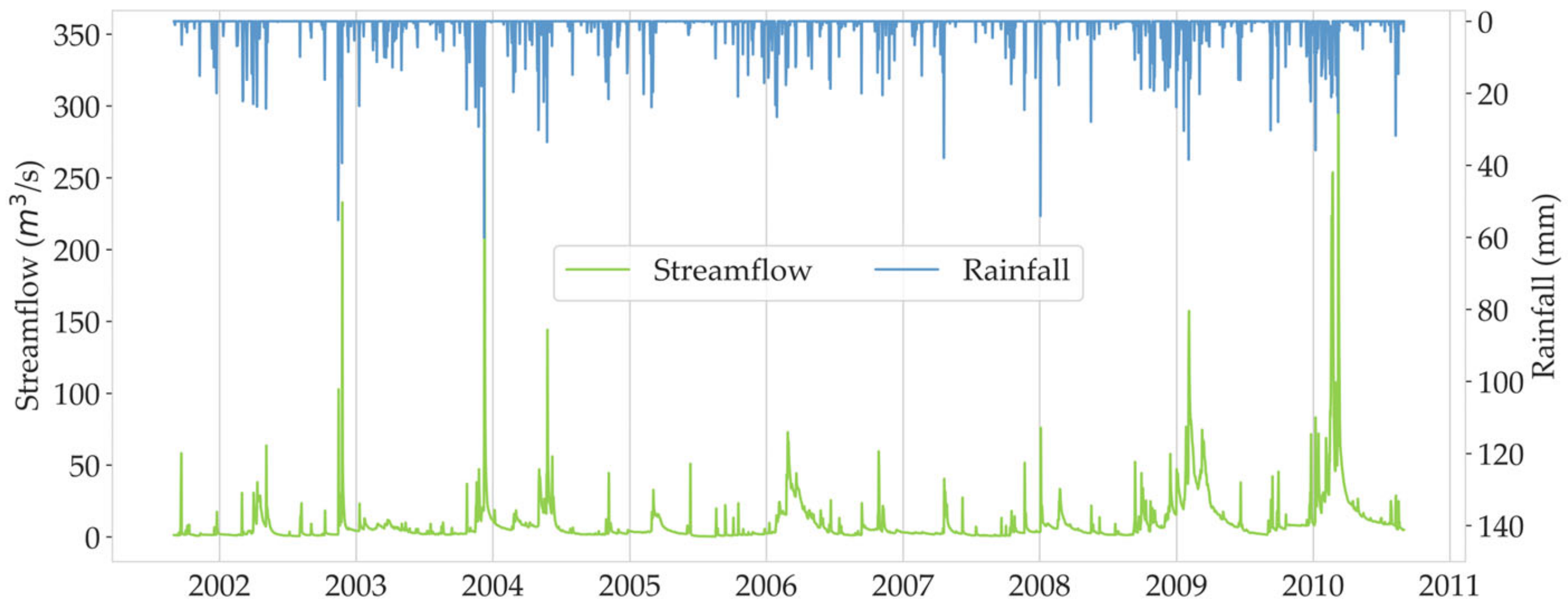
2.2. Data
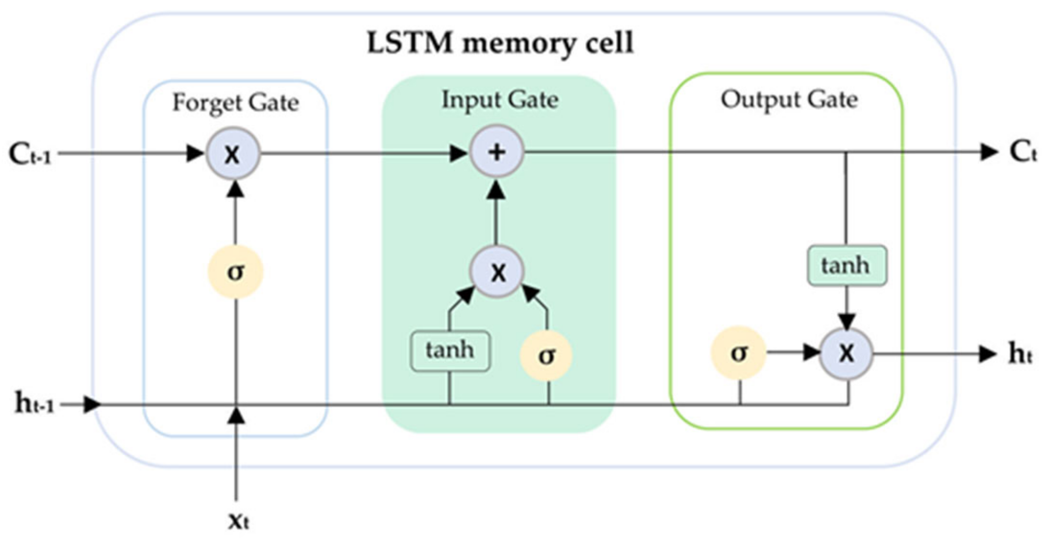
2.3. Long Short-Term Memory (LSTM)
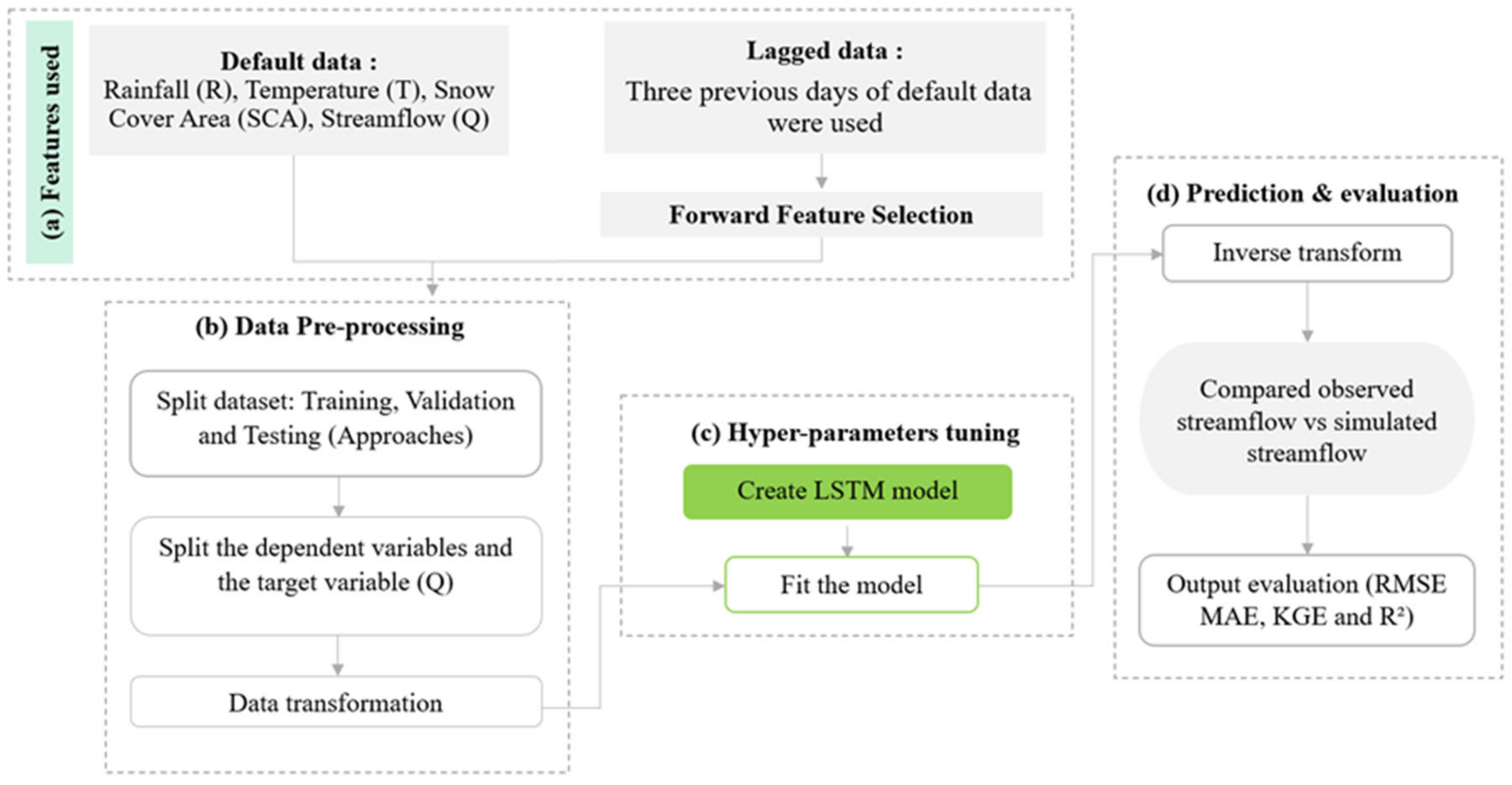
2.4. Methodology
2.4.1. Feature Selection
2.4.2. Data Pre-Processing
- Approach 2: splitting data taking into consideration the hydrological year that started from September of the current year and ended in August. Six years for training (1 September 2001–31 August 2007), one year and 6 months for validation (1 September 2007–28 February 2009), and one year and 6 months for testing (1 March 2009–31 August 2010).
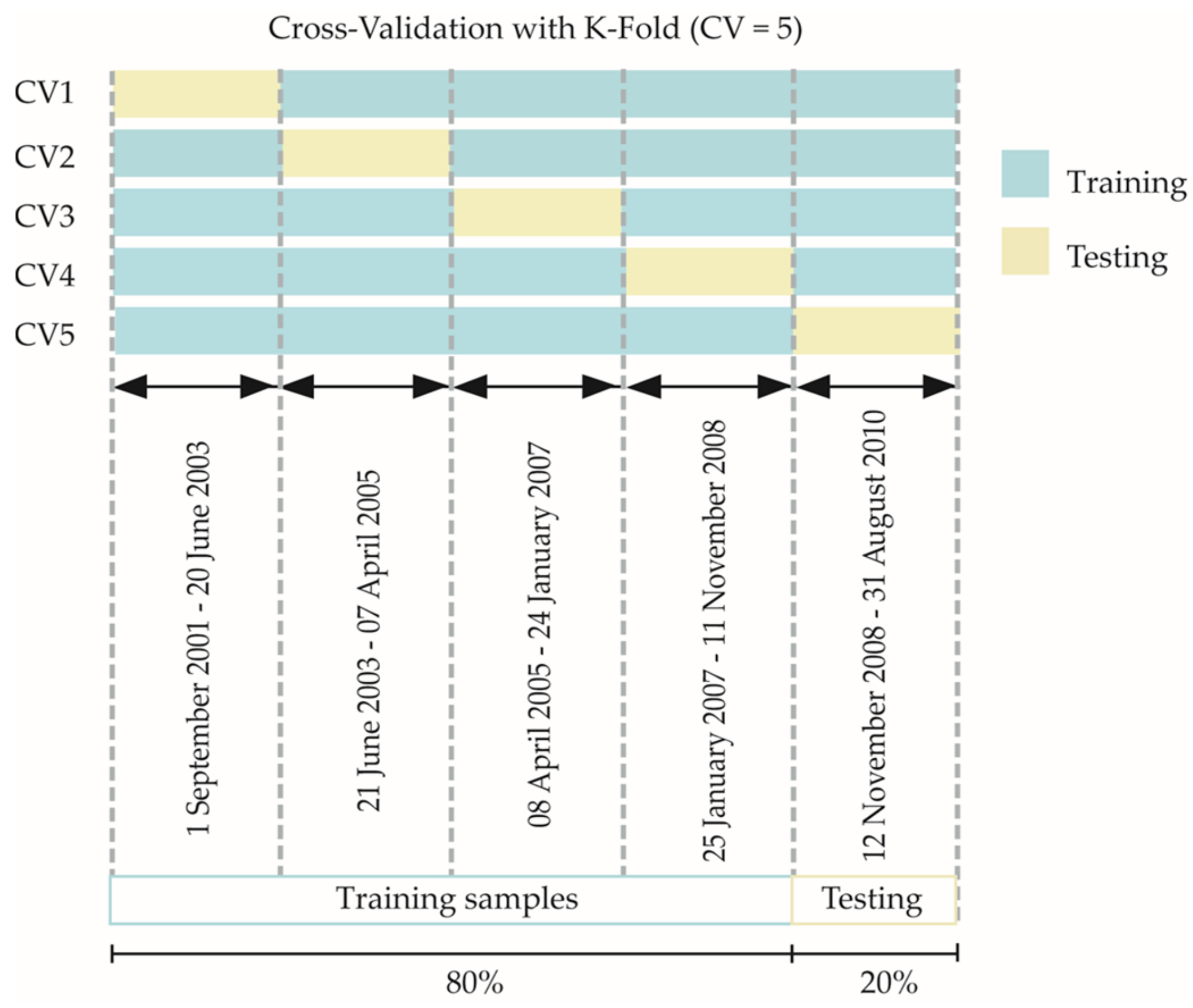
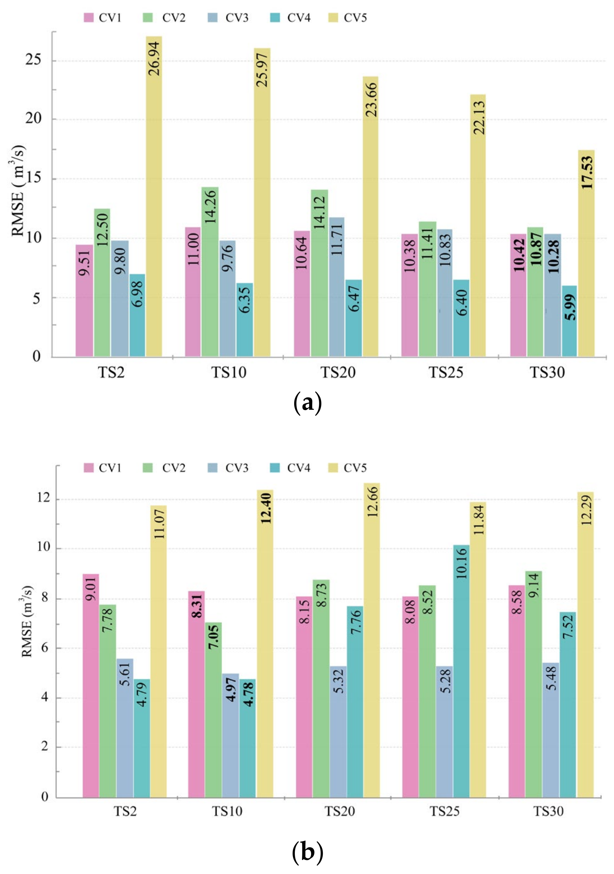
- Approach 3: with limited data samples, k-fold cross-validation is the most widely used method to assess the model’s performance. It divides the dataset in k equal-sized numbers, with one out of k parts is used as the testing set while the model is trained using k-1 folds [43]. The configuration of the cross-validation parameter is referred as the number of split iterations that the dataset will be divided into. Overall, it is from 2 to 10 depending on the availability of the data. In this study, we tested the different values of cross-validation (CV). The appropriate value is CV = 5 with 80% as the training set (7 years), along with 20% of the train data as the validation set and 20% for testing (2 years) in each group that was employed (Figure 5).
2.4.3. Hyper-Parameter Tuning
2.4.4. Model Evaluation Criteria
3. Results and Discussion
3.1. Evaluation of Model Performance Using Random Split
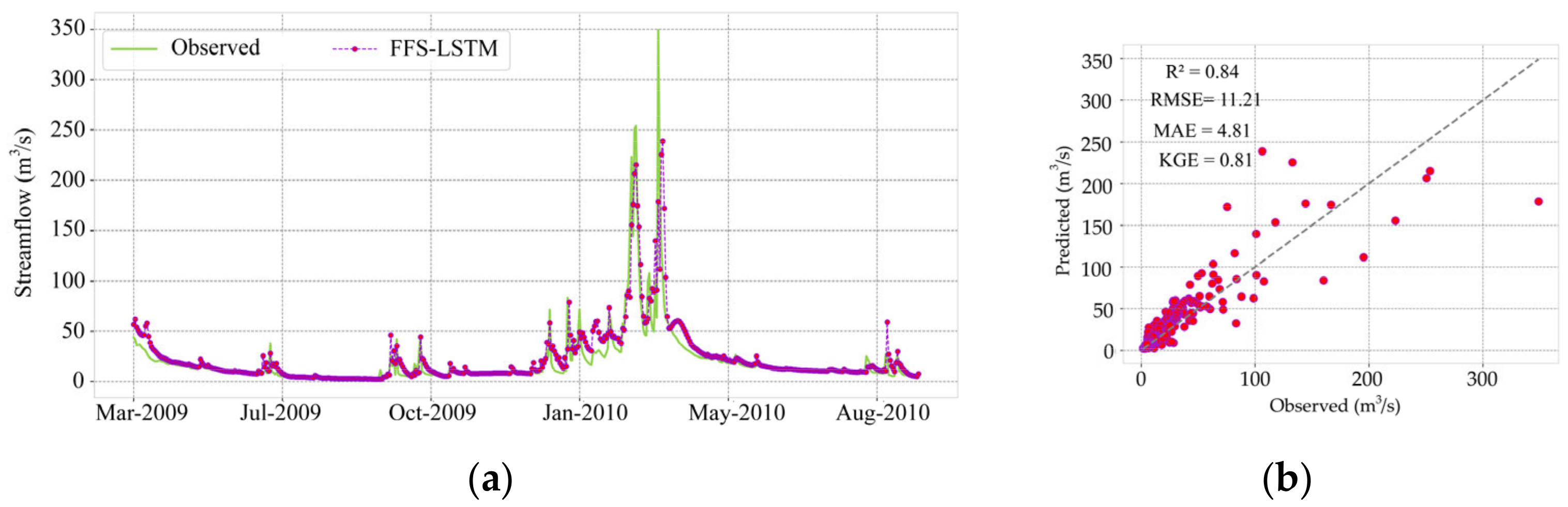
3.2. Evaluation of Model Performance with Automatically Split
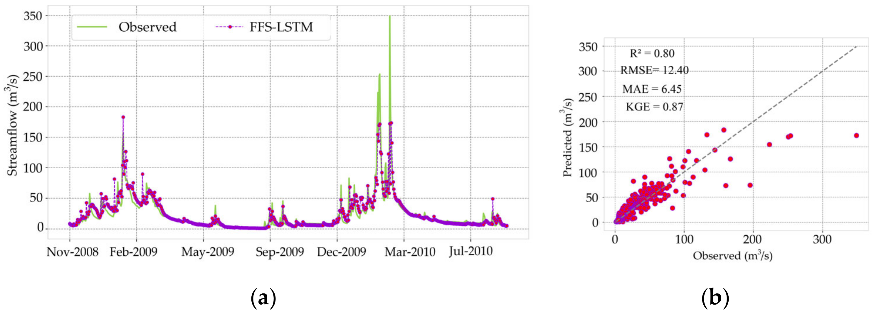
3.3. Reliability of LSTM Model
4. Conclusions
Author Contributions
Funding
Data Availability Statement
Acknowledgments
Conflicts of Interest
References
- Fniguire, F.; Laftouhi, N.; Saidi, M.; Zamrane, Z.; El Himer, H.; Khalil, N. Spatial and temporal analysis of the drought vulnerability and risks over eight decades in a semi-arid region (Tensift basin: Morocco). Theor. Appl. Climatol. 2017, 130, 321–330. [Google Scholar] [CrossRef]
- Zkhiri, W.; Tramblay, Y.; Hanich, L.; Jarlan, L.; Ruelland, D. Spatiotemporal characterization of current and future droughts in the High Atlas basins (Morocco). Theor. Appl. Climatol. 2019, 135, 593–605. [Google Scholar] [CrossRef]
- Ouatiki, H.; Boudhar, A.; Tramblay, Y.; Jarlan, L.; Benabdelouhab, T.; Hanich, L.; El Meslouhi, M.R.; Chehbouni, A. Evaluation of TRMM 3B42 V7 rainfall product over the Oum Er Rbia watershed in Morocco. Climate 2017, 5, 1. [Google Scholar] [CrossRef]
- Jarlan, L.; Khabba, S.; Er-Raki, S.; Le Page, M.; Hanich, L.; Fakir, Y.; Merlin, O.; Mangiarotti, S.; Gascoin, S.; Ezzahar, J.; et al. Remote Sensing of Water Resources in Semi-Arid Mediterranean Areas: The joint international laboratory TREMA. Int. J. Remote Sens. 2015, 36, 4879–4917. [Google Scholar] [CrossRef]
- Apaydin, H.; Sattari, M.T.; Falsafian, K.; Prasad, R. Artificial intelligence modelling integrated with Singular Spectral analysis and Seasonal-Trend decomposition using Loess approaches for streamflow predictions. J. Hydrol. 2021, 600, 126506. [Google Scholar] [CrossRef]
- Boudhar, A.; Ouatiki, H.; Bouamri, H.; Lebrini, Y.; Karaoui, I.; Hssaisoune, M.; Arioua, A.; Benabdelouahab, T. Hydrological Response to Snow Cover Changes Using Remote Sensing over the Oum Er Rbia Upstream Basin, Morocco; Springer International Publishing: Berlin/Heidelberg, Germany, 2020. [Google Scholar]
- Besaw, L.; Rizzo, D.; Bierman, P.; Hackett, W. Advances in ungauged streamflow prediction using artificial neural networks. J. Hydrol. 2010, 386, 27–37. [Google Scholar] [CrossRef]
- Devi, G.; Ganasri, B.; Dwarakish, G. A Review on Hydrological Models. Aquat. Procedia 2015, 4, 1001–1007. [Google Scholar] [CrossRef]
- Ouatiki, H.; Boudhar, A.; Ouhinou, A.; Beljadid, A.; Leblanc, M.; Chehbouni, A. Sensitivity and interdependency analysis of the HBV conceptual model parameters in a semi-arid mountainous watershed. Water 2020, 12, 2440. [Google Scholar] [CrossRef]
- Hu, C.; Wu, Q.; Li, H.; Jian, S.; Li, N.; Lou, Z. Deep learning with a long short-term memory networks approach for rainfall-runoff simulation. Water 2018, 10, 1543. [Google Scholar] [CrossRef] [Green Version]
- Yang, S.; Yang, D.; Chen, J.; Santisirisomboon, J.; Lu, W.; Zhao, B. A physical process and machine learning combined hydrological model for daily streamflow simulations of large watersheds with limited observation data. J. Hydrol. 2020, 590, 125206. [Google Scholar] [CrossRef]
- Botsis, D.; Latinopoulos, P.; Diamantaras, K. Rainfall–Runoff Modeling Using Support Vector Regression and Artificial Neural Networks. Cest2011 2011, No. January. Available online: http://aetos.it.teithe.gr/~kdiamant/docs/CEST2011.pdf (accessed on 2 November 2022).
- Chanklan, R.; Kaoungku, N.; Suksut, K.; Kerdprasop, K.; Kerdprasop, N. Runoff prediction with a combined artificial neural network and support vector regression. Int. J. Mach. Learn. Comput. 2018, 8, 39–43. [Google Scholar] [CrossRef] [Green Version]
- Hadi, S.; Tombul, M. Forecasting Daily Streamflow for Basins with Different Physical Characteristics through Data-Driven Methods. Water Resour. Manag. 2018, 32, 3405–3422. [Google Scholar] [CrossRef]
- Parisouj, P.; Mohebzadeh, H.; Lee, T. Employing Machine Learning Algorithms for Streamflow Prediction: A Case Study of Four River Basins with Different Climatic Zones in the United States. Water Resour. Manag. 2020, 34, 4113–4131. [Google Scholar] [CrossRef]
- Ha, S.; Liu, D.; Mu, L. Prediction of Yangtze River streamflow based on deep learning neural network with El Niño–Southern Oscillation. Sci. Rep. 2021, 11, 1–23. [Google Scholar] [CrossRef]
- Lai, G. Modeling Long- and Short-Term Temporal Patterns with Deep Neural Networks. In Proceedings of the 41st International ACM SIGIR Conference on Research & Development in Information Retrieval, Ann Arbor, MI, USA, 8–12 July 2018; pp. 95–104. [Google Scholar]
- Hu, J.; Wang, X.; Zhang, Y.; Zhang, D.; Zhang, M.; Xue, J. Time Series Prediction Method Based on Variant LSTM Recurrent Neural Network. Neural Process. Lett. 2020, 52, 1485–1500. [Google Scholar] [CrossRef]
- Hochreiter, S.; Schmidhuber, J. Long Short-Term Memory. Neural Comput. 1997, 9, 1735–1780. [Google Scholar] [CrossRef]
- Kratzert, F.; Klotz, D.; Brenner, C.; Schulz, K.; Herrnegger, M. Rainfall-Runoff modelling using Long-Short-Term-Memory (LSTM) networks. Hydrol. Earth Syst. Sci. Discuss. 2018, 22, 1–26. [Google Scholar] [CrossRef] [Green Version]
- Boulmaiz, T.; Guermoui, M.; Boutaghane, H. Impact of training data size on the LSTM performances for rainfall–runoff modeling. Model. Earth Syst. Environ. 2020, 6, 2153–2164. [Google Scholar] [CrossRef]
- Kao, I.; Zhou, Y.; Chang, L.; Chang, F. Exploring a Long Short-Term Memory based Encoder-Decoder framework for multi-step-ahead flood forecasting. J. Hydrol. 2020, 583, 124631. [Google Scholar] [CrossRef]
- Apaydin, H.; Feizi, H.; Sattari, M.; Colak, M.; Shamshirband, S.; Chau, K. Comparative analysis of recurrent neural network architectures for reservoir inflow forecasting. Water 2020, 12, 1500. [Google Scholar] [CrossRef]
- Cheng, M.; Fang, F.; Kinouchi, T.; Navon, I.; Pain, C. Long lead-time daily and monthly streamflow forecasting using machine learning methods. J. Hydrol. 2020, 590, 125376. [Google Scholar] [CrossRef]
- Mao, G.; Wang, M.; Liu, J.; Wang, Z.; Wang, K.; Meng, Y.; Zhong, R.; Wang, H.; Li, Y. Comprehensive comparison of artificial neural networks and long short-term memory networks for rainfall-runoff simulation. Phys. Chem. Earth 2021, 123, 103026. [Google Scholar] [CrossRef]
- Ouma, Y.; Cheruyot, R.; Wachera, A. Rainfall and runoff time-series trend analysis using LSTM recurrent neural network and wavelet neural network with satellite-based meteorological data: Case study of Nzoia hydrologic basin. Complex Intell. Syst. 2021, 8, 213–236. [Google Scholar] [CrossRef]
- Li, W.; Kiaghadi, A.; Dawson, C. High temporal resolution rainfall–runoff modeling using long-short-term-memory (LSTM) networks. Neural Comput. Appl. 2020, 33, 1261–1278. [Google Scholar] [CrossRef]
- Prediction, S. Learning Enhancement Method of Long Short-Term Memory Network and Its Applicability in Hydrological Time Series Prediction. Water 2022, 14, 2910. [Google Scholar]
- Kratzert, F.; Klotz, D.; Herrnegger, M.; Sampson, A.; Hochreiter, S.; Nearing, G. Toward Improved Predictions in Ungauged Basins: Exploiting the Power of Machine Learning. Water Resour. Res. 2019, 55, 11344–11354. [Google Scholar] [CrossRef] [Green Version]
- Choi, J.; Lee, J.; Kim, S. Utilization of the Long Short-Term Memory network for predicting streamflow in ungauged basins in Korea. Ecol. Eng. 2022, 182, 106699. [Google Scholar] [CrossRef]
- Hunt, K.; Matthews, G.; Pappenberger, F.; Prudhomme, C. Using a long short-term memory (LSTM) neural network to boost river streamflow forecasts over the western United States. Hydrol. Earth Syst. Sci. Discuss. 2022, 26, 5449–5472. [Google Scholar] [CrossRef]
- Rahimzad, M.; Nia, A.M.; Zolfonoon, H.; Soltani, J.; Mehr, A.D.; Kwon, H. Performance Comparison of an LSTM-based Deep Learning Model versus Conventional Machine Learning Algorithms for Streamflow Forecasting. Water Resour. Manag. 2021, 35, 4167–4187. [Google Scholar] [CrossRef]
- Park, K.; Jung, Y.; Kim, K. Determination of Deep Learning Model and Optimum Length of Training Data in the River with Large Fluctuations in Flow Rates. Water 2020, 12, 3537. [Google Scholar] [CrossRef]
- El Bilali, A.; Taleb, A.; Brouziyne, Y. Groundwater quality forecasting using machine learning algorithms for irrigation purposes. Agric. Water Manag. 2021, 245, 106625. [Google Scholar] [CrossRef]
- Ouatiki, H.; Boudhar, A.; Ouhinou, A.; Arioua, A.; Hssaisoune, M.; Bouamri, H.; Benabdelouahab, T. Trend analysis of rainfall and drought over the Oum Er-Rbia River Basin in Morocco during 1970–2010. Arab. J. Geosci. 2019, 12, 128. [Google Scholar] [CrossRef]
- Ouakhir, H.; El Ghachi, M.; Goumih, M.; Hamid, L. Fluvial Dynamic in Oued El Abid Basin: Monitoring and Quantification at an Upstream River Section in Bin El Ouidane Dam—2016/2017-(Central High Atlas/Morocco). Am. J. Mech. Appl. 2020, 8, 47. [Google Scholar] [CrossRef]
- Marchane, A.; Jarlan, L.; Hanich, L.; Boudhar, A.; Gascoin, S.; Tavernier, A.; Filali, N.; Le Page, M.; Hagolle, O.; Berjamy, B. Assessment of daily MODIS snow cover products to monitor snow cover dynamics over the Moroccan Atlas mountain range. Remote Sens. Environ. 2015, 160, 72–86. [Google Scholar] [CrossRef]
- Uysal, G.; Şensoy, A.; Şorman, A. Improving daily streamflow forecasts in mountainous Upper Euphrates basin by multi-layer perceptron model with satellite snow products. J. Hydrol. 2016, 543, 630–650. [Google Scholar] [CrossRef]
- Thapa, S.; Zhao, Z.; Li, B.; Lu, L.; Fu, D.; Shi, X.; Tang, B.; Qi, H. Snowmelt-driven streamflow prediction using machine learning techniques (LSTM, NARX, GPR, and SVR). Water 2020, 12, 1734. [Google Scholar] [CrossRef]
- Boudhar, A.; Hanich, L.; Boulet, G.; Duchemin, B.; Berjamy, B.; Chehbouni, A. Evaluation of the Snowmelt Runoff model in the Moroccan High Atlas Mountains using two snow-cover estimates. Hydrol. Sci. J. 2009, 54, 1094–1113. [Google Scholar] [CrossRef] [Green Version]
- Fan, H.; Jiang, M.; Xu, L.; Zhu, H.; Cheng, J.; Jiang, J. Comparison of long short term memory networks and the hydrological model in runoff simulation. Water 2020, 12, 175. [Google Scholar] [CrossRef] [Green Version]
- Lee, D.; Lee, G.; Kim, S.; Jung, S. Future runoff analysis in the mekong river basin under a climate change scenario using deep learning. Water 2020, 12, 1556. [Google Scholar] [CrossRef]
- Kim, T.; Yang, T.; Gao, S.; Zhang, L.; Ding, Z.; Wen, X.; Gourley, J.J.; Hong, Y. Can artificial intelligence and data-driven machine learning models match or even replace process-driven hydrologic models for streamflow simulation? A case study of four watersheds with different hydro-climatic regions across the CONUS. J. Hydrol. 2021, 598, 126423. [Google Scholar] [CrossRef]
- Reis, G.B.; Da Silva, D.D.; Fernandes Filho, E.I.; Moreira, M.C.; Veloso, G.V.; De Souza Fraga, M.; Pinheiro, S.A.R. Effect of environmental covariable selection in the hydrological modeling using machine learning models to predict daily streamflow. J. Environ. Manag. 2021, 290, 112625. [Google Scholar] [CrossRef] [PubMed]
- Ren, K.; Fang, W.; Qu, J.; Zhang, X.; Shi, X. Comparison of eight fi lter-based feature selection methods for monthly stream fl ow forecasting—Three case studies on CAMELS data sets. J. Hydrol. 2020, 586, 124897. [Google Scholar] [CrossRef]
- Singh, D.; Singh, B. Investigating the impact of data normalization on classification performance. Appl. Soft Comput. 2020, 97, 105524. [Google Scholar] [CrossRef]
- Bai, P.; Liu, X.; Xie, J. Simulating runoff under changing climatic conditions: A comparison of the long short-term memory network with two conceptual hydrologic models. J. Hydrol. 2021, 592, 125779. [Google Scholar] [CrossRef]
- Ahmed, S.; Rahman, S.; San, O.; Rasheed, A.; Navon, I. Memory embedded non-intrusive reduced order modeling of non-ergodic flows. Phys. Fluids 2019, 31, 126602. [Google Scholar] [CrossRef] [Green Version]
- Almalaq, A.; Zhang, J. Evolutionary Deep Learning-Based Energy Consumption Prediction for Buildings. IEEE Access 2019, 7, 1520–1531. [Google Scholar] [CrossRef]
- Liu, C.; Gu, J.; Yang, M. A Simplified LSTM Neural Networks for One Day-Ahead Solar Power Forecasting. IEEE Access 2021, 9, 17174–17195. [Google Scholar] [CrossRef]
- Fu, M.; Fan, T.; Ding, Z.; Salih, S.; Al-Ansari, N.; Yaseen, Z. Deep Learning Data-Intelligence Model Based on Adjusted Forecasting Window Scale: Application in Daily Streamflow Simulation. IEEE Access 2020, 8, 32632–32651. [Google Scholar] [CrossRef]
- Hu, Y.; Yan, L.; Hang, T.; Feng, J. Stream-flow forecasting of small rivers based on LSTM. arXiv 2020, arXiv:2001.05681. [Google Scholar]
- Zhang, D.; Liu, X.; Bai, P.; Li, X. Suitability of satellite-based precipitation products for water balance simulations using multiple observations in a humid catchment. Remote Sens. 2019, 11, 151. [Google Scholar] [CrossRef] [Green Version]
- Knoben, W.; Freer, J.; Woods, R. Technical note: Inherent benchmark or not? Comparing Nash-Sutcliffe and Kling-Gupta efficiency scores. Hydrol. Earth Syst. Sci. 2019, 23, 4323–4331. [Google Scholar] [CrossRef] [Green Version]
- Bouabid, R.; Chafai, A.; Alaoui, E.; Bahri, H. Streamflow response to climate variability in sub-watersheds of the Sebou river basin, Morocco. In Proceedings of the EGU General Assembly 2010, Vienna, Austria, 2–7 May 2010; p. 3237. [Google Scholar]
- Ávila, L.; Silveira, R.; Campos, A.; Rogiski, N.; Gonçalves, J.; Scortegagna, A.; Freita, C.; Aver, C.; Fan, F. Comparative Evaluation of Five Hydrological Models in a Large-Scale and Tropical River Basin. Water 2022, 14, 3013. [Google Scholar] [CrossRef]


| Watershed | Area (km2) | Perimeter | Altitude Min | Altitude Max | Altitude Mean | Principal River |
|---|---|---|---|---|---|---|
| Ait Ouchen | 2427 | 322 | 953 | 3230 | 1945 | Oued El Abid |
| Scenarios | Variables Description |
|---|---|
| LSTM | rainfall (R), temperature (T) and snow cover area (SCA) |
| FFS-LSTM | rainfall, lagged rainfall (1, 2 days), 3 lagged days of streamflow and 2, 3 days lagged SCA |
| Hyper-Parameters | Selection | |
|---|---|---|
| Create LSTM | Neurons in the input layer | 50 neurons |
| Neurons in the hidden layer | 20 neurons | |
| Neurons in the output layer | One neuron | |
| Fit LSTM | Activation function | tanh |
| Number of Epochs | 250 epochs | |
| Batch size | 10, 32 | |
| Loss function Optimizer | Mean Square Error Adam |
| Scenarios | Training | Validation | Testing | |||||||||
|---|---|---|---|---|---|---|---|---|---|---|---|---|
| RMSE | MAE | KGE | R2 | RMSE | MAE | KGE | R2 | RMSE | MAE | KGE | R2 | |
| LSTM | ||||||||||||
| TS2 TS10 TS20 TS25 TS30 | 9.30 | 4.52 | 0.30 | 0.43 | 18.86 | 10.40 | −0.65 | 0.07 | 31.86 | 14.06 | −2.77 | 0.04 |
| 7.44 | 3.77 | 0.65 | 0.63 | 17.69 | 9.86 | −0.81 | 0.19 | 29.32 | 13.66 | −1.88 | 0.20 | |
| 7.49 | 3.80 | 0.72 | 0.63 | 15.38 | 9.20 | −0.12 | 0.39 | 27.98 | 13.22 | −1.24 | 0.29 | |
| 8.85 | 5.14 | 0.54 | 0.48 | 14.18 | 9.50 | 0.52 | 0.48 | 26.27 | 14.07 | −1.07 | 0.35 | |
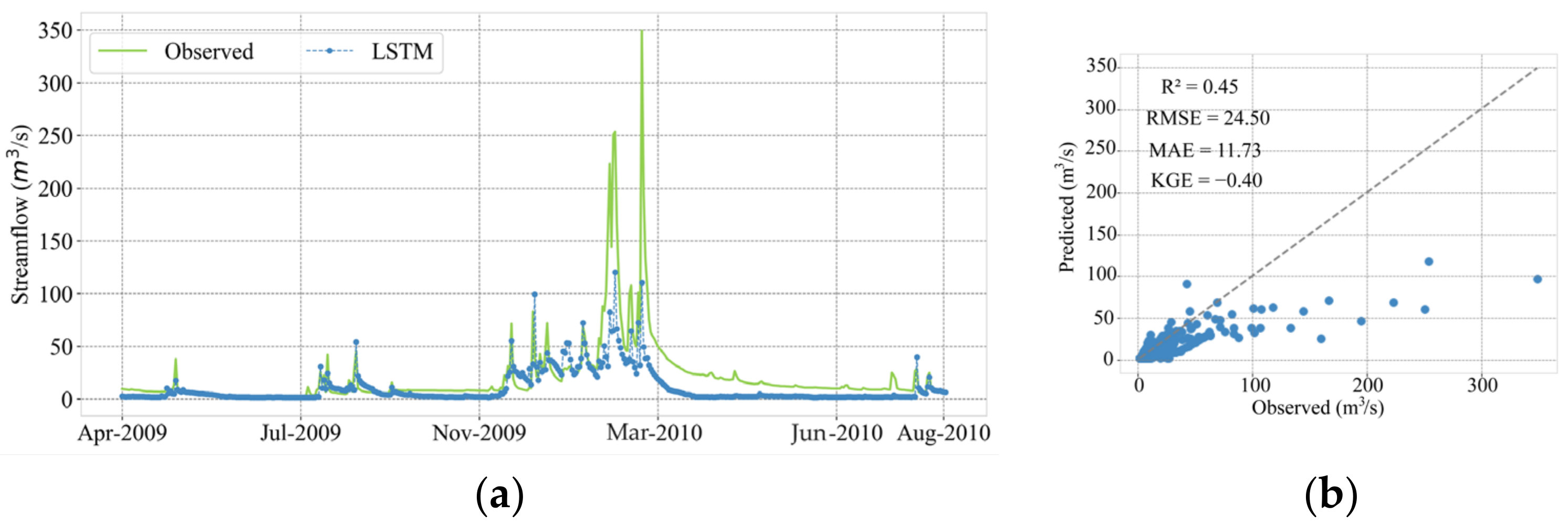
| 6.13 | 3.23 | 0.83 | 0.75 | 14.52 | 8.57 | 0.02 | 0.46 | 24.50 | 11.73 | −0.40 | 0.45 | |
| FFS-LSTM | ||||||||||||
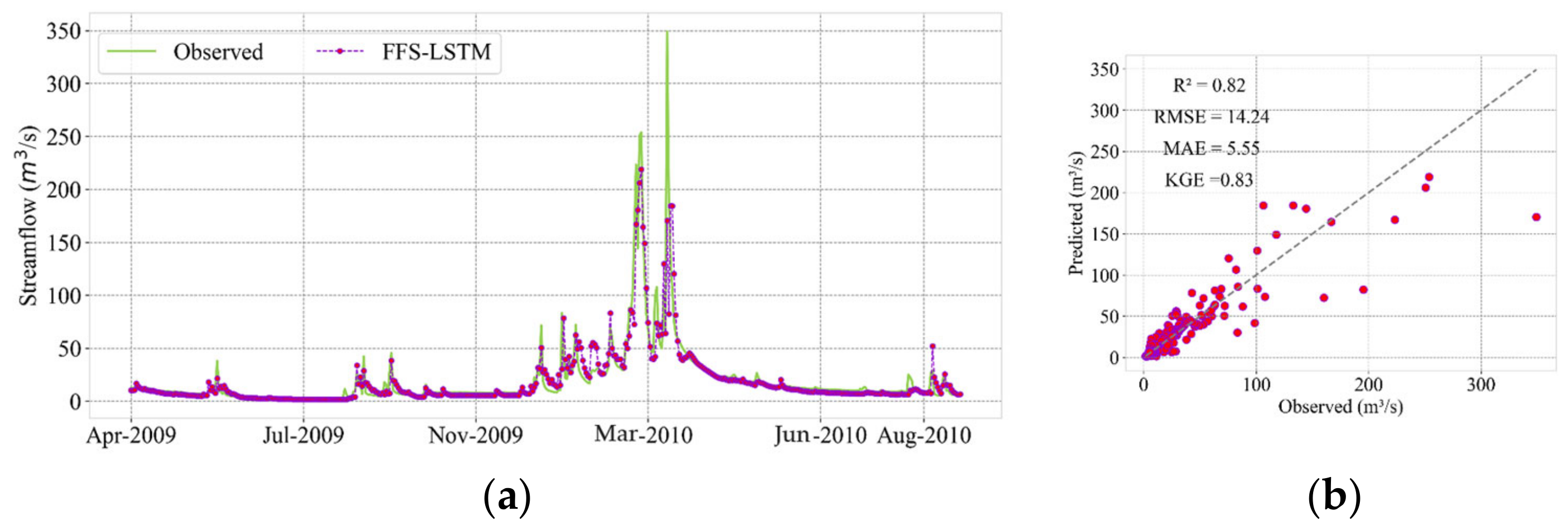
| TS2 TS10 TS20 TS25 TS30 | 5.64 | 2.28 | 0.90 | 0.79 | 8.85 | 4.26 | 0.84 | 0.80 | 15.08 | 5.41 | 0.72 | 0.78 |
| 5.21 | 2.15 | 0.88 | 0.82 | 9.27 | 4.62 | 0.82 | 0.78 | 14.24 | 5.55 | 0.83 | 0.82 | |
| 5.86 | 2.54 | 0.82 | 0.77 | 12.05 | 6.20 | 0.67 | 0.63 | 14.86 | 6.35 | 0.88 | 0.79 | |
| 4.21 | 1.86 | 0.93 | 0.88 | 8.25 | 4.05 | 0.70 | 0.83 | 19.77 | 6.76 | 0.10 | 0.64 | |
| 5.16 | 2.36 | 0.90 | 0.82 | 9.74 | 5.72 | 0.76 | 0.75 | 14.69 | 6.07 | 0.79 | 0.80 | |
| Scenarios | Training | Validation | Testing | |||||||||
|---|---|---|---|---|---|---|---|---|---|---|---|---|
| RMSE | MAE | KGE | R2 | RMSE | MAE | KGE | R2 | RMSE | MAE | KGE | R2 | |
| LSTM | ||||||||||||
| TS2 TS10 TS20 TS25 TS30 | 9.59 | 4.16 | 0.26 | 0.42 | 10.90 | 5.82 | 0.31 | 0.29 | 29.58 | 15.00 | −2.39 | −0.04 |
| 8.83 | 4.55 | 0.57 | 0.56 | 10.13 | 5.82 | 0.44 | 0.39 | 27.35 | 14.10 | −1.43 | 0.13 | |
| 8.17 | 4.80 | 0.54 | 0.58 | 10.49 | 6.39 | 0.30 | 0.35 | 24.39 | 12.39 | −1.09 | 0.22 | |
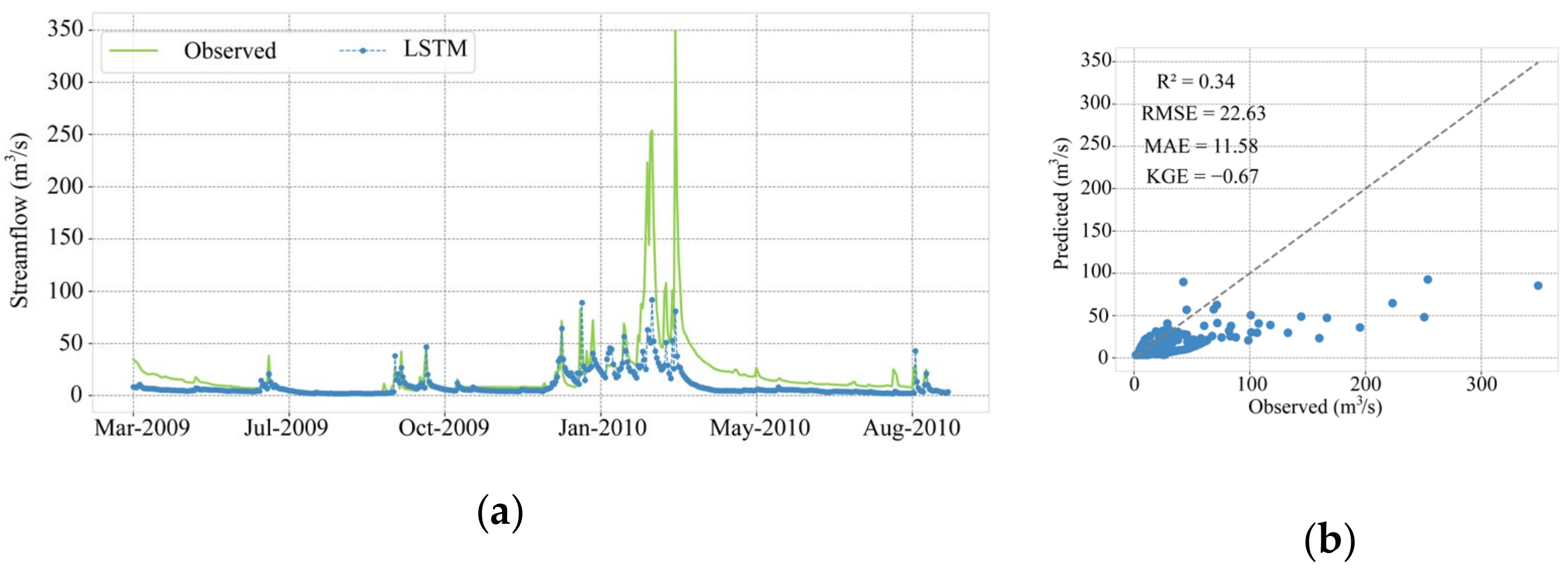
| 6.81 | 4.01 | 0.74 | 0.71 | 9.21 | 5.24 | 0.58 | 0.51 | 22.63 | 11.58 | −0.67 | 0.34 | |
| 8.47 | 4.80 | 0.48 | 0.55 | 11.32 | 6.64 | 0.02 | 0.25 | 23.92 | 11.87 | −1.05 | 0.25 | |
| FFS-LSTM | ||||||||||||
| TS2 TS10 TS20 TS25 TS30 | 7.09 | 2.74 | 0.75 | 0.68 | 7.57 | 3.63 | 0.75 | 0.66 | 13.87 | 5.57 | 0.76 | 0.78 |
| 6.33 | 2.72 | 0.79 | 0.75 | 8.53 | 4.01 | 0.72 | 0.57 | 14.82 | 5.95 | 0.86 | 0.75 | |
| 4.83 | 2.62 | 0.78 | 0.85 | 7.97 | 4.06 | 0.76 | 0.63 | 11.21 | 4.81 | 0.81 | 0.84 | |
| 5.52 | 2.52 | 0.78 | 0.81 | 7.34 | 3.77 | 0.78 | 0.69 | 11.31 | 4.50 | 0.75 | 0.84 | |
| 5.80 | 2.93 | 0.75 | 0.78 | 9.22 | 4.80 | 0.66 | 0.51 | 10.95 | 5.17 | 0.84 | 0.83 | |
| Scenario | Training | Validation | Testing | |||||||||
|---|---|---|---|---|---|---|---|---|---|---|---|---|
| RMSE | MAE | KGE | R2 | RMSE | MAE | KGE | R2 | RMSE | MAE | KGE | R2 | |
| LSTM | ||||||||||||
| CV1 | 11.4 | 5.72 | −0.39 | 0.37 | 26.32 | 12.56 | −3.03 | 0.06 | 10.42 | 4.45 | −0.43 | 0.2 |
| CV2 | 8.27 | 5.27 | 0.38 | 0.6 | 23.55 | 11.56 | −1.34 | 0.25 | 10.87 | 5.44 | 0.12 | 0.55 |
| CV3 | 7.14 | 4.54 | 0.63 | 0.77 | 23.26 | 11.33 | −1.24 | 0.27 | 10.28 | 6.29 | 0.45 | 0.01 |
| CV4 | 8.91 | 5.98 | 0.43 | 0.66 | 22.68 | 10.8 | −1.04 | 0.3 | 5.99 | 4.99 | 0.4 | 0.28 |
| CV5 | 8.1 | 4.86 | 0.62 | 0.6 | 6.13 | 4.13 | 0.58 | 0.28 | 17.53 | 10.41 | 0.54 | 0.58 |
| Scenario | Training | Validation | Testing | |||||||||
|---|---|---|---|---|---|---|---|---|---|---|---|---|
| RMSE | MAE | KGE | R2 | RMSE | MAE | KGE | R2 | RMSE | MAE | KGE | R2 | |
| FFS-LSTM | ||||||||||||
| CV1 | 5.1 | 2.12 | 0.75 | 0.87 | 12.71 | 4.95 | 0.48 | 0.78 | 8.31 | 2.28 | 0.26 | 0.51 |
| CV2 | 4.98 | 2.62 | 0.86 | 0.85 | 13.3 | 4.73 | 0.45 | 0.76 | 7.05 | 2.9 | 0.7 | 0.8 |
| CV3 | 5.26 | 2.5 | 0.87 | 0.87 | 14.11 | 5.63 | 0.3 | 0.73 | 4.97 | 2.24 | 0.8 | 0.77 |
| CV4 | 5.8 | 3.48 | 0.65 | 0.85 | 13.27 | 6.8 | 0.5 | 0.76 | 4.78 | 3.1 | −0.01 | 0.53 |
| CV5 | 6.01 | 2.64 | 0.8 | 0.78 | 4.47 | 2.04 | 0.8 | 0.62 | 12.4 | 6.45 | 0.87 | 0.8 |
Disclaimer/Publisher’s Note: The statements, opinions and data contained in all publications are solely those of the individual author(s) and contributor(s) and not of MDPI and/or the editor(s). MDPI and/or the editor(s) disclaim responsibility for any injury to people or property resulting from any ideas, methods, instructions or products referred to in the content. |
© 2023 by the authors. Licensee MDPI, Basel, Switzerland. This article is an open access article distributed under the terms and conditions of the Creative Commons Attribution (CC BY) license (https://creativecommons.org/licenses/by/4.0/).
Share and Cite
Nifa, K.; Boudhar, A.; Ouatiki, H.; Elyoussfi, H.; Bargam, B.; Chehbouni, A. Deep Learning Approach with LSTM for Daily Streamflow Prediction in a Semi-Arid Area: A Case Study of Oum Er-Rbia River Basin, Morocco. Water 2023, 15, 262. https://doi.org/10.3390/w15020262
Nifa K, Boudhar A, Ouatiki H, Elyoussfi H, Bargam B, Chehbouni A. Deep Learning Approach with LSTM for Daily Streamflow Prediction in a Semi-Arid Area: A Case Study of Oum Er-Rbia River Basin, Morocco. Water. 2023; 15(2):262. https://doi.org/10.3390/w15020262
Chicago/Turabian StyleNifa, Karima, Abdelghani Boudhar, Hamza Ouatiki, Haytam Elyoussfi, Bouchra Bargam, and Abdelghani Chehbouni. 2023. "Deep Learning Approach with LSTM for Daily Streamflow Prediction in a Semi-Arid Area: A Case Study of Oum Er-Rbia River Basin, Morocco" Water 15, no. 2: 262. https://doi.org/10.3390/w15020262