
Performance of Semi-Active Flapping Hydrofoil with Arc Trajectory


1
School of Ocean Engineering, Harbin Institute of Technology, Weihai 264209, China
2
School of Mechanical and Material Engineering, North China University of Technology, No. 5 Jinyuanzhuang Road, Beijing 100144, China
3
Department of Naval Architecture, Ocean and Marine Engineering, Strathclyde University, Glasgow G4 0LZ, UK
*
Author to whom correspondence should be addressed.
Water 2023, 15(2), 269; https://doi.org/10.3390/w15020269
Submission received: 8 December 2022
/
Revised: 3 January 2023
/
Accepted: 4 January 2023
/
Published: 9 January 2023
(This article belongs to the Section Hydraulics and Hydrodynamics)
Abstract
:The semi-active flapping foil driven by the swing arm is a simple structure to realize the propulsion of the flapping foil. The motion trajectory of this semi-active flapping foil mechanism is a circular arc, and its hydrodynamic characteristics are not clear. This paper systematically investigates the working characteristics and hydrodynamic performance of this semi-active flapping foil with a circular arc track. Compared with the traditional flapping foil structure, the special design parameters of the semi-active flapping foil driven by the swing arm mainly include the length of the swing arm and the stiffness of the torsion spring. In this paper, the three-dimensional fluid-structure coupling method is used by solving the fluid dynamics equation and the structural dynamics equation, and the working characteristics of the structure with different motion and geometric parameters are analyzed. From the results, increasing the swing arm length is beneficial to improving the peak efficiency of the flapping foil, and also to improving the thrust coefficient corresponding to the peak efficiency point. Under a certain swing arm length, reducing the spring stiffness is also conducive to improving the peak efficiency of the propulsion system, but it is adverse to the thrust coefficient. Further analysis shows that the maximum angle of attack is the key factor affecting the efficiency of this flapping foil propulsion. For the flapping foil described in this paper, its peak efficiency is usually concentrated near . However, for the thrust coefficient of this kind of flapping foil propulsion, the influencing factors are relatively complex, including swinging arm, the spring stiffness, and the advance coefficient. The maximum angle of attack remains the key factor affecting the peak thrust in the range of advance coefficient far from the starting state.
1. Introduction
Fish and aquatic mammals have beautifully evolved to be able to utilize the physical principles of unsteady hydrodynamics to achieve both high maneuverability and high propulsive efficiency [1]. Taking inspiration from the natural swimmers, a variety of structures such as bionic fish or bionic limbs have emerged, and have attracted much attention due to their high efficiency and high mobility.
Among biomimetic propulsion, there are roughly three structural forms. One is a common fish structure that achieved propulsion by swinging its tails and bodies, such as tuna [2,3], solar rain [4], and zebrafish [5]; another is a kind of structure propelled by twisting the body, such as eel [6,7] and snake [8]; still others are propelled by flapping wide wings, such as manta rays [9]. Additionally, bionic limb structures are mainly in the form of bionic turtles [10] and bionic penguins [11]. In general, the realization of these biomimetic propulsion systems depends on complex mechanisms and special materials, so the engineering application is difficult and economic.
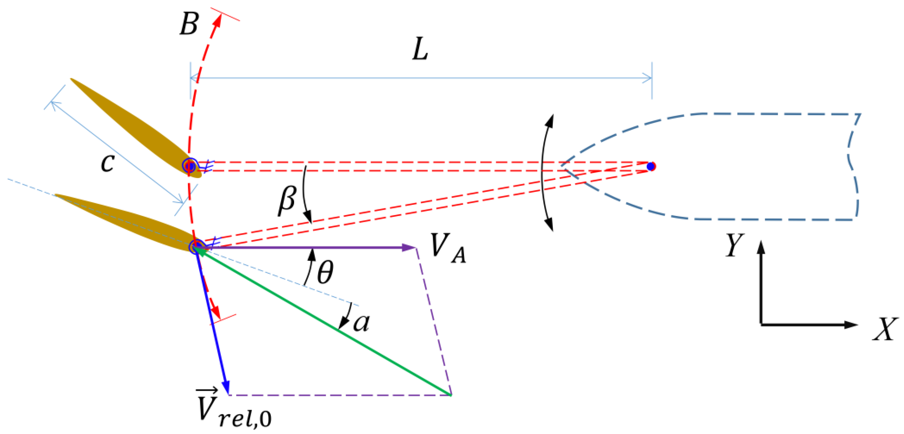
Because the tails of some of the fastest swimming animals closely resemble high-aspect-ratio foils, flapping hydrofoils have been studied extensively using theoretical and numerical techniques [12]. Typical flapping foil propulsion is a rigid flapping foil with two degrees of freedom, which is composed of simple harmonic heave motion and pitch motion [13,14]. This rigid flapping foil with two degrees of freedom has been well studied and the highest efficiency of about 87% has been reached [14,15,16]. Whereas, some studies have also reminded the disadvantages of this kind of fully prescribed flapping foil propulsion, e.g., the amount of energy lost and mechanical complication since it requires mechanically coupled and constrained two motions through complex mechanisms [17]. Owing to the low efficiency of a single degree-of-freedom flapping hydrofoil [18,19], a semi-active flapping hydrofoil with only one actuator is proposed and required by the researchers [20]. Since the heave motion of oscillating foil propulsion generates most of the thrust, the actively imposed motion is usually the heave motion, while the pitch motion is determined by a special structure or material [16,17,21]. While ensuring high propulsion efficiency, the semi-active propulsion system, therefore, promises a more feasible approach in engineering projects compared to the fully prescribed-motion foil system. One semi-active implementation method is to use the torsion spring on the foil to control the pitch motion. When the flapping foil is pitching under the action of the hydrodynamic moment, its pitching angle is determined by torsion spring force, hydrodynamic force, and inertial force, so that it can work at a certain angle of attack [17,21,22]. Such a flow-adjusted pitching motion is expected to decrease the instantaneous flow separation and simplify the controlling mechanism. On this basis, this paper proposes a semi-active flapping hydrofoil system driven by a swing arm [23]. With this structure, the flapping hydrofoil can be installed at the tail of the vehicles and driven by the reciprocating swinging arm, as shown in Figure 1. It has the advantages of a simple structure, low water tightness requirements, and high engineering reliability.
Owing to the introduction of the torsion spring, the spring force, mass force, and hydrodynamic force constitute a new spring-mass system. Therefore, the dynamic response of such a semi-active flapping foil system is complicated, and very much dependent on the various system kinematic and structural parameters [24,25], including the torsional spring stiffness, the flapping foil inertia, the hydrodynamic-added inertia, etc. At the same time, different from the traditional semi-active flapping hydrofoil, the motion trajectory of this semi-active flapping foil driven by the swing arm is a circular arc. According to some studies on the flapping hydrofoil trajectory [26,27], the motion trajectory could have a significant impact on the hydrodynamic performance of system. Although the research on semi-active flapping foil propulsion has gone through a relatively comprehensive discussion during the past decades, to the authors’ knowledge, there is still a lack of comprehensive parametric analysis regarding semi-active flapping hydrofoil systems driven by a swing arm, up until now. In view of this, based on our work on the parameters of the semi-active flapping hydrofoil [28], we conduct a three-dimensional (3D) investigation into the influence of multiple motions and geometry parameters on the propulsive characteristics of semi-active flapping hydrofoil driven by the swing arm. It aims to provide essential implications and guidance for this propulsion system in marine applications. The outline of the rest of the paper is as follows. We begin by describing the geometric structure, motion and kinematic, and dynamic parameters of a semi-active flapping hydrofoil driven by the swing arm in Section 2. Then, the fluid–structure coupling numerical method is described and fully verified in Section 3. In Section 4, a systematic presentation on the simulation results is included. Our particular interest is centered on the influence of the arm length (L/c) and torsion spring stiffness (K) on the propulsive performance, including propulsion force, propulsive efficiency, and related wake structure. A systematic and parametric analysis is conducted to correlate the influencing factors to the propulsive performance. Additionally, the sensitivity of the performance on the variation in several governing parameters is also evaluated in the current study.
2. Description and Definition of Flapping Foil Propulsion
2.1. Geometric Structure and Motion
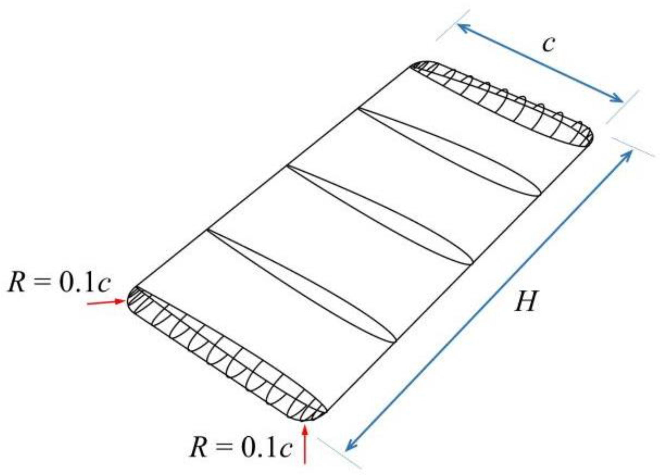
This semi-active flapping hydrofoil propulsion system includes a rigid foil and an arm connecting the foil-pitching axis to the base, as shown schematically in Figure 1. The flapping foil and the arm are elastically connected at the pitching axis by a torsion spring. A rigid 3D airfoil is used, with the chord length and the spanwise H = 0.2 m. The NACA0012 airfoil is used, and the 3D flapping hydrofoil is designed with equal chord length. Round corners are designed at both ends of the span direction of the flapping hydrofoil, with a radius of R = 0.1 c, and connected with an elliptic curve to form the end shape, as shown in Figure 2.
The flapping hydrofoil is driven by a swing arm mounted on the hull, and the swing arm is driven to and fro with a swing angle (β) by the power device in the hull, as shown in Figure 1. The arm length is varied in this study and denoted as L. The swing angle (β) adopts the sine curve, which can be expressed as
where is the maximum swing angle of the swing arm and is the swing frequency of the swing arm. In all the examples in this paper, the swing frequency is set as .
The other end of the swing arm is connected the flapping hydrofoil with a torsion spring. When the system is stationary and does not work, the chord line of the airfoil coincides with the swing arm. During operation, when affected by the combined action of inertia moment, spring moment, and hydrodynamic moment in the pitching direction, the flapping foil works at a pitching angle (θ). It is the included angle between the flapping foil and the X-axis, as shown in Figure 1. Additionally, the heave motion (driven by the swing arm) together with the advance velocity creates an oscillating hydrodynamic force and moment causing the flapping foil to work at an angle of attack α (AoA). The torsion spring is used to restore the flapping foil toward the equilibrium position. In addition, the flapping foil does not have any other degrees of freedom. The dynamic equation of the semi-active flapping foil rotating about the axis can be written as
where I is the rotational inertia about the axis of the flapping hydrofoil considering the attached water, ; K denotes torsion spring stiffness, Nm/rad; Mz denotes the fluid moment imposed on foil, N.m; and is the pitching angle, radian.
According to relation with the pitching angle (θ) and the foil speed relative to the hull (Vrel,0), shown in Figure 1, the AoA of flapping foil at different times can be expressed as Equation (3). The maximum AoA in a period of motion can be expressed as .
where and are velocity components of the pitching center speed of the foil relative to the hull (Vrel,0), which can be obtained according to the movement of the swinging arm; is the speed of the hull, which is a constant value under a certain working condition.
In the numerical simulation described herein, the pitching center of flapping foil is set at the leading edge of the airfoil, which was adopted in the research of Thaweewat et al. [17]. The range of VA used in this study is 0.2~4 m/s. The advance coefficient J of the semi-active flapping foil is about 0.67 to 15, and the corresponding Re is about 2 × 10⁵~9 × 10⁵. The rotational inertia () around the axis is related to the frequency ratio of the pitching motion of the flapping foil. In our previous studies [28], the effect of the resonance mechanism on the semi-active flapping foil performance was studied. The analysis of varying frequency ratio showed that the system resonance makes the foil deviate from the ideal angle of attack and the propulsion performance of the system declines or even loses propulsion entirely. When the frequency ratio is small, that is, the foil has a small moment of inertia, the self-pitching flapping foil can work well. A more suitable frequency ratio could be selected below 0.5. Considering that the effect on the flapping foil performance is very small when the frequency ratio is small [28], we set rotational inertia I = 0.001 Kgm2 in all the examples described in this paper. Additionally, it has been verified that the performance of the flapping foil is almost not affected by rotational inertia near this value.
2.2. Nondimensional Propulsive Indicators
In order to systematically analyze the performance of the flapping foil, the hull is set to move along the X-axis at different constant speeds () without other degrees of freedom, so as to obtain the thrust and efficiency of the semi-active propulsion system at different speeds. These dimensionless parameters used in this paper are defined as follows.
For the flapping-frequency dimensionless processing, St number is used, which is expressed by Equation (4).
For tFor the convenience in comparing marine propellers, Floc’h [29] introduced the advance coefficient (J), as shown in Equation (5), which is adopted in this paper. It is the reciprocal of St number.
Referring to the definition of the screw propeller thrust coefficient and the definition method of Floc’h [29], this paper chose the swept area B·H instead of the foil extension area c·H as the reference area for the flapping foils. Following the practice in the maritime industry, the thrust coefficient (KT) is redefined as Equation (6).
where represents the characteristic velocity, represents the swept area, represents the arc length between the top and bottom dead points of the swing arm arc motion, and represents the average thrust in the forward direction, which is expressed as
where T represents the period of the flapping hydrofoil, s.
The input power of the flapping foil can be obtained according to the action of the pitching center on the foil and the movement of the pitching center, which can be expressed as
where , , and are represented as the X-direction force, Y-direction force, and torque exerted by the swing arm on the pitching center of flapping foil, respectively, and is the swing angular velocity of the swing arm.
The output power of the flapping foil propeller is the product of the advancing velocity (VA) and the average thrust (). Therefore, the efficiency of the flapping foil is defined as the ratio of output power () to input power (), which is expressed as Equation (9)
The Definitions for all the parameters involved in this paper are provided in Table 1.
3. Computational Method and Validation
A 3D numerical model for simulating the semi-active flapping hydrofoil with arc trajectory was implemented on the CFD software FINE/Marine (a software package of NUMECA, the EURANUS solver was developed by the European Space Agency). This solver adopts internal implicit iteration within a time-step iteration to ensure strong flow/motion coupling. The main features of the model—the governing equations, mesh and boundary conditions, turbulence modeling, and validation—are discussed in this section.
3.1. Governing Equations
The dynamic equation of semi-active flapping hydrofoil propulsion was introduced above in Equation (2). By using the integral incompressible viscous fluid dynamics equation, considering the motion of grid cells and without considering the influence of gravity, the hydrodynamic equation can be written as follows.
where Ω is the element volume; is the flow velocity; is velocity component of ; is the sum of viscous stress and Reynolds stress( The turbulent viscosity coefficient is determined by Menter’s k-ω shear–stress transport turbulent model [30]); p is the pressure; Sj is the components of area vector ; and is the density of water.
3.2. Mesh and Method
The computational domain simulates a water tunnel with 4 m width, 4 m height, and 8 m length test section, as shown in Figure 3. The viscous effect of the water tunnel wall is ignored, and the four outside boundary conditions are set as slip wall. The right-side inlet boundary has a given inflow velocity and pressure. The gradient of pressure and velocity at the left-side outlet boundary is set as zero. The setting methods for the boundary conditions are shown in Figure 3.
As it is a preliminary discussion, this paper neglects the resistance influence of the swing arm and focuses on the ideal state of the mechanism. Therefore, the swing arm is simplified as a rigid connection between the flapping foil shaft and the base shaft on the hull. The flapping hydrofoil is located at the center of the water tunnel, 2 m away from the entrance. The swinging arm and the hull are both virtual objects, and no entity appears in the numerical analysis. Only the flapping foil is placed in the computational domain, and its movement is controlled by the motion parameters.
A hexahedron grid with local successive refinement method applied is chosen for the computational domain to maintain the local region as a refined mesh; the enlarged detail of the grid near the foil surface is shown in Figure 3. To accurately simulate the pressure and velocity gradient on the foil surface and the separated vortex in the trail, further mesh refinement is carried out on the foil surface and its surrounding area. The refined mesh size is shown in Table 2. The grid size of each region listed in Table 2 is the maximum grid size of the area, and most actual grid sizes are smaller, which ensure the accuracy of this simulation. The refined near-wall mesh ensures that the y+ value is about 1.0. The dual time-stepping method is used for the transient simulation, and the k-ω turbulence model, which is widely used in aviation, is adopted in the simulation. In order to adapt to the large-scale compound motion of the foil, the elastic twist grid technology is also adopted in the calculation. The deformation of the grid during the operation of the flapping foil can be roughly seen in the enlarged detail of Figure 3. We performed extensive work on the grid verification for the flapping hydrofoil [16,28,31] in the early stage, so it is not repeated here.
3.3. Validation
To validate the numerical method used in the current work, two validation parts are carried out in this part, including the time-step verification and the simulation verification of selected benchmark conditions, as described in Read’s [32] and Schoveiler’s [33] experiments.
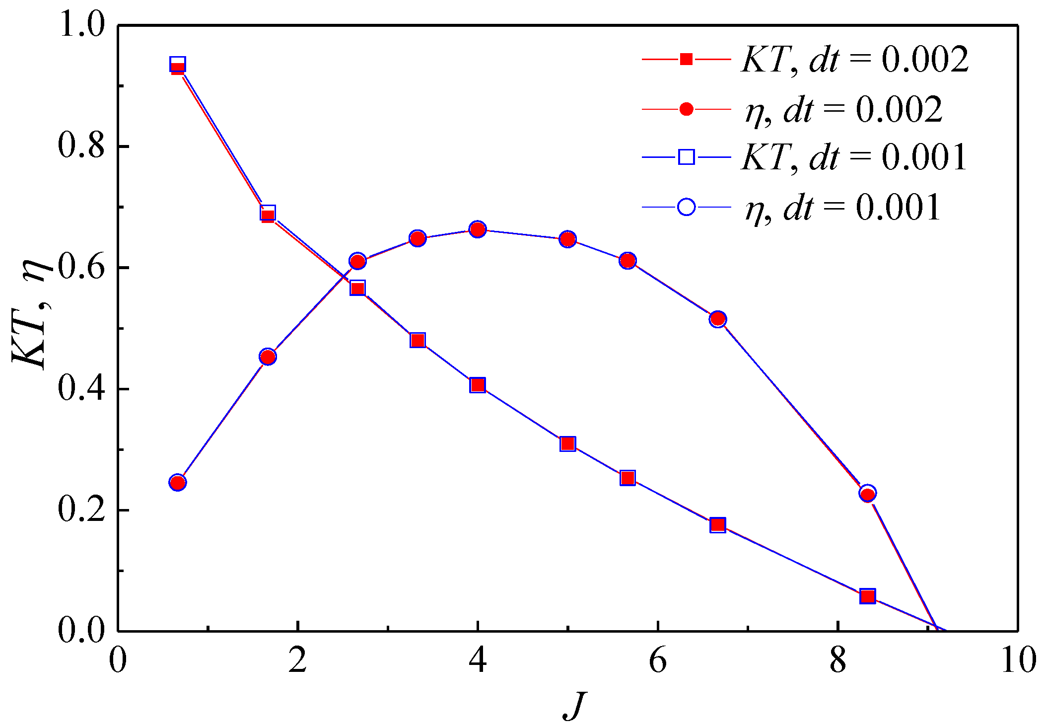
The flow field formed by flapping-foil motion is a strong unsteady flow field accompanied by flow separation [33]. Considering the influence of time step on the simulation accuracy of unsteady separated flow, comparative analysis of two time steps Δt/T = 0.0005 and 0.001 for the same working conditions is initially carried out in this section. The selected working condition is and . The k-ω turbulence model is used and the comparison results are shown in Figure 4. In this figure, blue and red lines represent the simulation results for different time steps. The rectangular and circular lines represent the KT and η curves, respectively. It can be seen from the figure that no matter the η or the KT, the two results in different time periods are in good agreement That is, the efficiency and thrust curves of the flapping foil almost coincide with each other under the two time-step settings of Δt/T = 0.002 and Δt/T = 0.001. Finally, the time step Δt/T = 0.002 (Δt/T = /500) for the following simulation is selected. Moreover, the sensitivity of the mesh analysis on the simulated results is also important, which is considered and studied throughout our work. Many results show that the grid size and area near the airfoil has a great effect on the performance of the flapping foil device. The verification of grid independence and the verification of the time step and turbulence model were both carried out and described in our previous work [28] and not repeated in this paper.
Although the flapping foil system studied herein is a 3D problem, because there are few experimental results on 3D flapping foil, this part only verifies the quasi-2D experiment results of Anderson [32] and Schoveiler [33], hoping to prove the feasibility of the numerical method presented in this paper. In their experiments, endplates were used on each strut to prevent flow around the ends of the foil and maintain approximately 2D flow [32]. In the future, the accuracy of the 3D method may be further discussed through 3D experiments or mutual verification with other 3D simulation results.
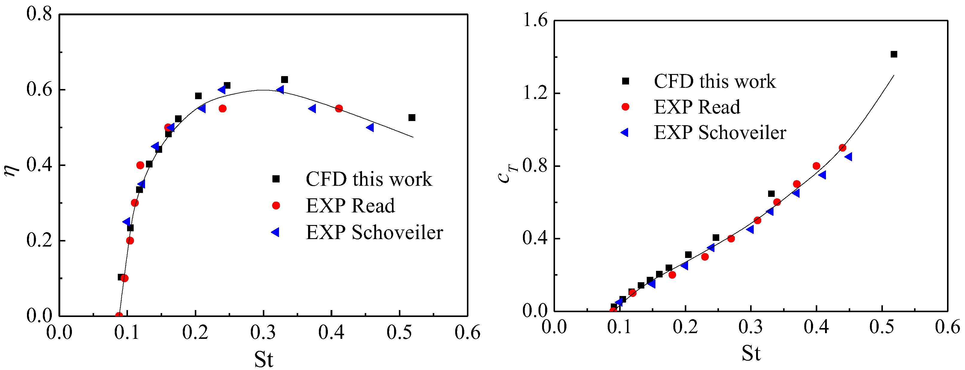
A rigid 2D NACA 0012 airfoil is used, and the motion is composed of active heave and pitch motion. The heave amplitude-to-chord ratio (y0/c) is 0.75, and the pitching axis is one-third chord from the leading edge of the foil. The experimental and the calculated results for f = 1.2 Hz and amax = 20° are compared and shown in Figure 5. The comparison presents excellent agreement between the two results in terms of the propulsive efficiency (η) and the thrust coefficient (cT). The definition of thrust coefficient given by Read et al. [32] and Schouveiler et al. [33] is slightly different from that presented in this paper, and the specific definition can be referred to the description in the literature.
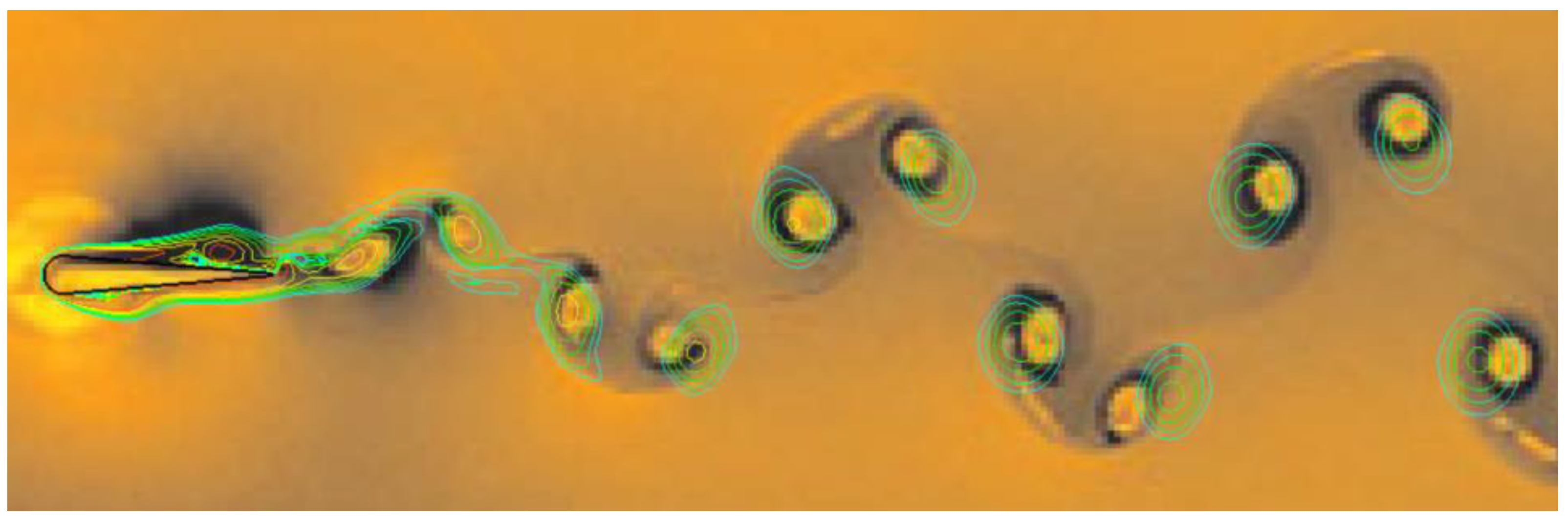
Subsequently, in order to verify the accuracy of the flow-field simulation in this method, the pure pitching and flapping foil measured by Schnipper et al. [18] was further simulated by the 2D method. The experiment was carried out with a very thin soap film, and the chord length of the flapping foil was also very small, only 6 mm. The soap film is a classical 2D flow because of the Re number. The experimental and calculated results are compared and shown in Figure 6. The shaded graph in Figure 6 shows the experimental results in the literature, and the contour graph is the 2D CFD results obtained in this paper. It can be seen that, on the whole, the simulation results of the wake core position are in good agreement with the experimental results, except for a few vortices away from the flapping foil.
4. Results and Analysis
Since this semi-active flapping hydrofoil is a spring–mass system, the torsional spring stiffness, the foil inertia, and the hydrodynamic-added inertia could affect the propulsive performance [25]. In this section, our particular interest is centered on the influence of arm length (L/c) and torsion spring stiffness (K) on the propulsive performance, including propulsion force, propulsive efficiency, and related wake structure.
4.1. Propulsive Efficiency and the Thrust Coefficient
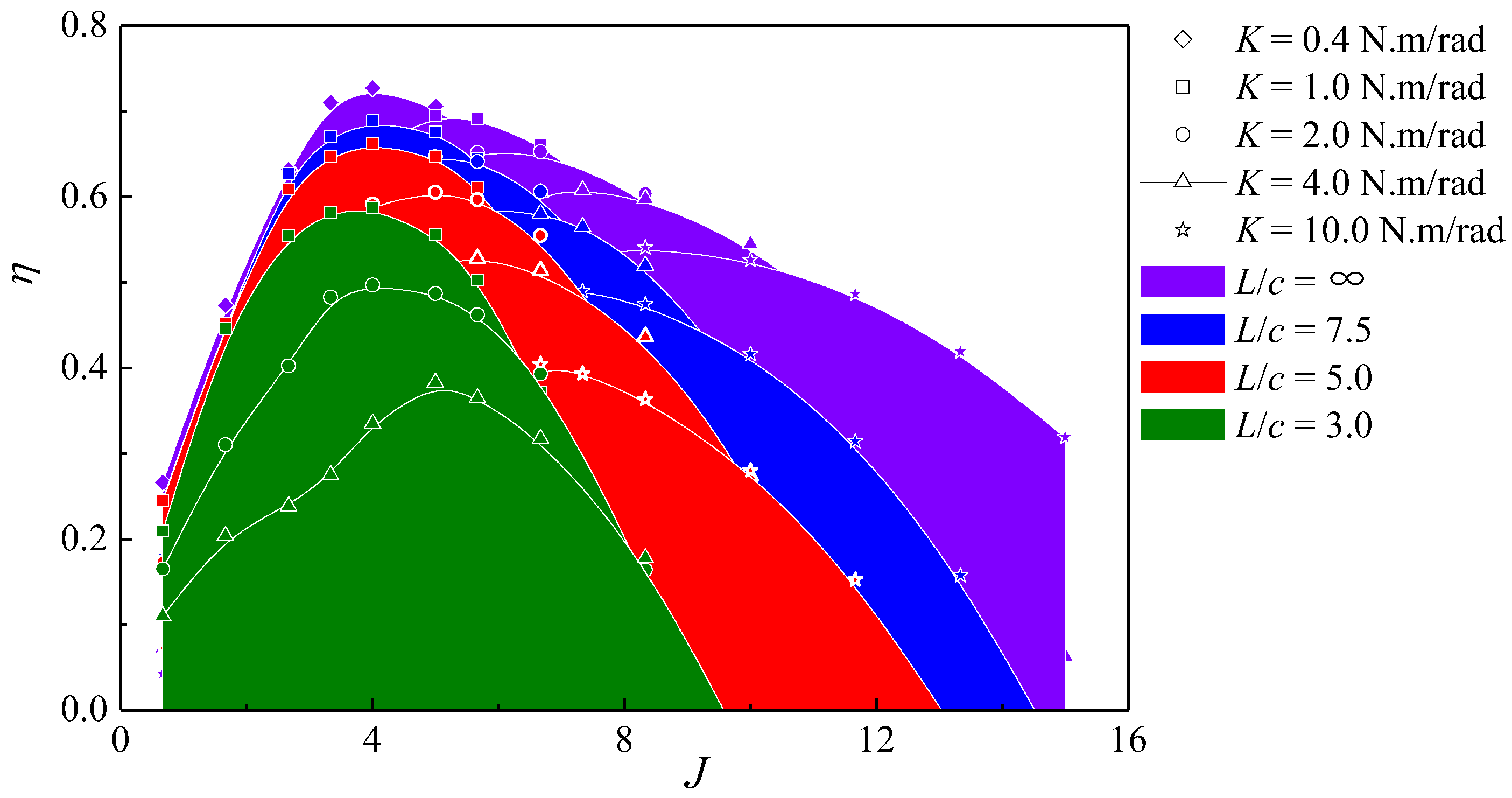
Firstly, the influence of arm length on the propulsive performance is observed; four cases are analyzed: . In order to compare, the swing arc length B of the swing arm under all working conditions is set to . That is, the maximum swing angle of swing arms () is different with different lengths. Considering that with different swing angles of the swing arm (), the effect of the torsion spring on the semi-active flapping hydrofoil is different. The effect of variable torsion spring stiffness K is also analyzed at the same time to show the influence of the arm length more comprehensively. With different swing arm lengths, five cases of torsion spring stiffness () are analyzed. The propulsive efficiency of the flapping foil with different arm lengths and spring stiffness is shown in Figure 7.
Firstly, from the results shown in Figure 7, the length of the swing arm has obvious influence on the peak efficiency and the efficient working range. With an increase in the swing arm, the peak efficiency with different spring stiffness is gradually improved, and the range of the efficient working point is correspondingly widened. In the case of , the maximum efficiency reaches 73%, which is slightly less than that of conventional semi-active flapping foil propulsion [28]. Secondly, the torsion spring stiffness (K) has an obvious effect on efficiency. With the increase in the spring stiffness, the peak efficiency decreases gradually, and the peak point moves to the direction of high advance coefficient (J). That is, with the same swing arm length, reducing the spring stiffness is conducive to improving the peak efficiency of this kind of flapping foil. This is because when the hydrodynamic moment received by the foil changes with the advance coefficient, if the spring stiffness is relatively small, then the pitch angle and AoA can more sensitively adapt to the change in torque, so as to achieve better working conditions; If the spring stiffness is relatively large, then the pitch angle and AoA cannot sensitively adapt to the change in torque. Therefore, within a section of the advance coefficient, the AoA is large and the efficiency continues to be low. Generally speaking, the sudden rise in the efficiency curve is due to the transition of the foil from a flow separation working state to a nonseparation working state [28].
It is worth noting that, with the increase in spring stiffness of the flapping foil, the propulsion system can maintain a satisfactory efficiency within a much wider range of advance coefficient. With reference to the work in Thaweewat [17], a dimensionless parameter, torsion spring stiffness ratio (K’), is the indicator used to describe the spring stiffness. It can be defined as
It can be seen from the formula that although the torsion spring stiffness (K) is fixed after design, the spring stiffness ratio K’ can be changed. That is, the position of the working point can be changed by adjusting the swing frequency f to adapt to the working conditions with different advance coefficients J. In other words, the propulsive performance of semi-active flapping propulsion is similar to that of a variable-pitch propeller [17]. However, we should also note that with the increase in spring stiffness, the efficiency peak shifts downward with the envelope to the right. That is, the semi-active flapping foil is beneficial for improving the high efficiency working range of the flapping foil propulsion, but has little effect on improving the peak efficiency.
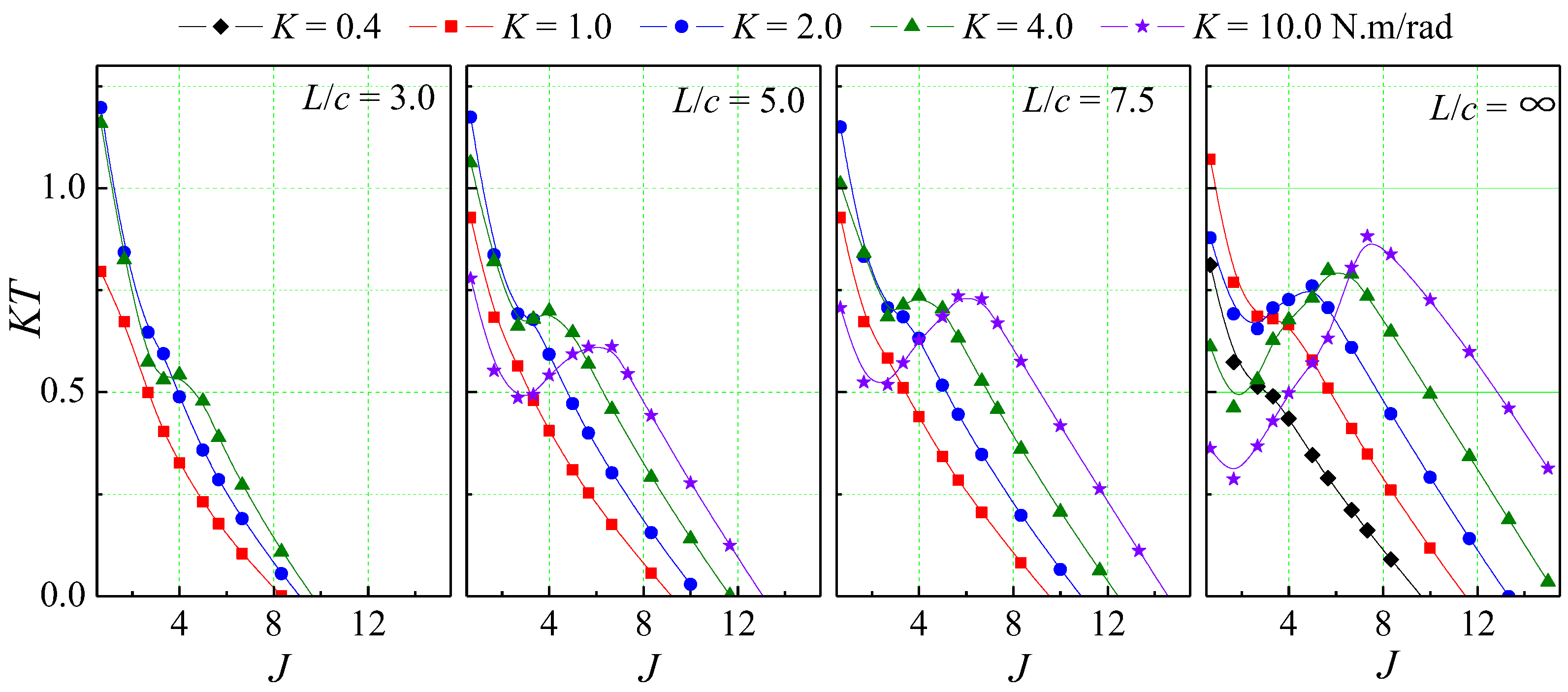
In addition to efficiency, thrust should also be considered in the design of flapping foil propulsion. The comparison results of thrust coefficient (KT) under different swing arm lengths and different spring stiffness are shown in Figure 8.
On the whole, except for that of the minimum swing arm length (L/c = 3.0), other thrust coefficient (KT) curves all show a peak value at higher advance coefficient (J), and a valley value and a small section of upwarping curve at lower advance coefficients. That is, compared with the conventional semi-active foil, the elliptical trajectory system also has a large thrust coefficient at low advance coefficient. However, under some low spring stiffness conditions (e.g., K = 0.4, K = 1.0), its peak and valley gradually disappear. This is consistent with the results we obtained in the study of conventional semi-active flapping foil propulsion [28]. In the details of this thrust coefficient curve, on the right-side of the peak value (that is, the high advance coefficients section), the thrust coefficient curve tends to shift to the upper right with the increase in spring stiffness. That is to say, under the working condition of high advance coefficients, it is more beneficial to select high spring stiffness to obtain a large thrust. Whereas, in the low advance coefficients section (on the left-side of the peak value), with the increase in the spring stiffness, KT tends to increase first and then decrease. In the case of , there is no trend in reduction because the greater spring stiffness is not calculated. In addition, at the beginning of the thrust coefficient curve, that is, in the foil start-up state (J < 2 in this paper), the thrust coefficient decreases gradually with the advance coefficient regardless of the spring stiffness.
The influence of swing arm length on the performance of the flapping foil is evident and clear. Under the same spring stiffness, the thrust coefficient of a larger arm length is larger and the peak value is higher. Moreover, with the increase in the swing arm length, the thrust performance of this semi-active flapping foil propulsion system gradually tends to the conventional semi-active flapping foil system. Considering the complex mechanism of thrust generation, which is closely related to the pitch angle, AoA and flow separation of the flapping foil, the following sections will further discuss AoA characteristic and flow separation of the system.
4.2. Angle of Attack Analysis
In addition to the advance coefficient, the spring stiffness ratio also affects the AoA of the flapping foil. Since the AoA varies periodically, maximum AoA (αmax) of each working condition is analyzed in this part.
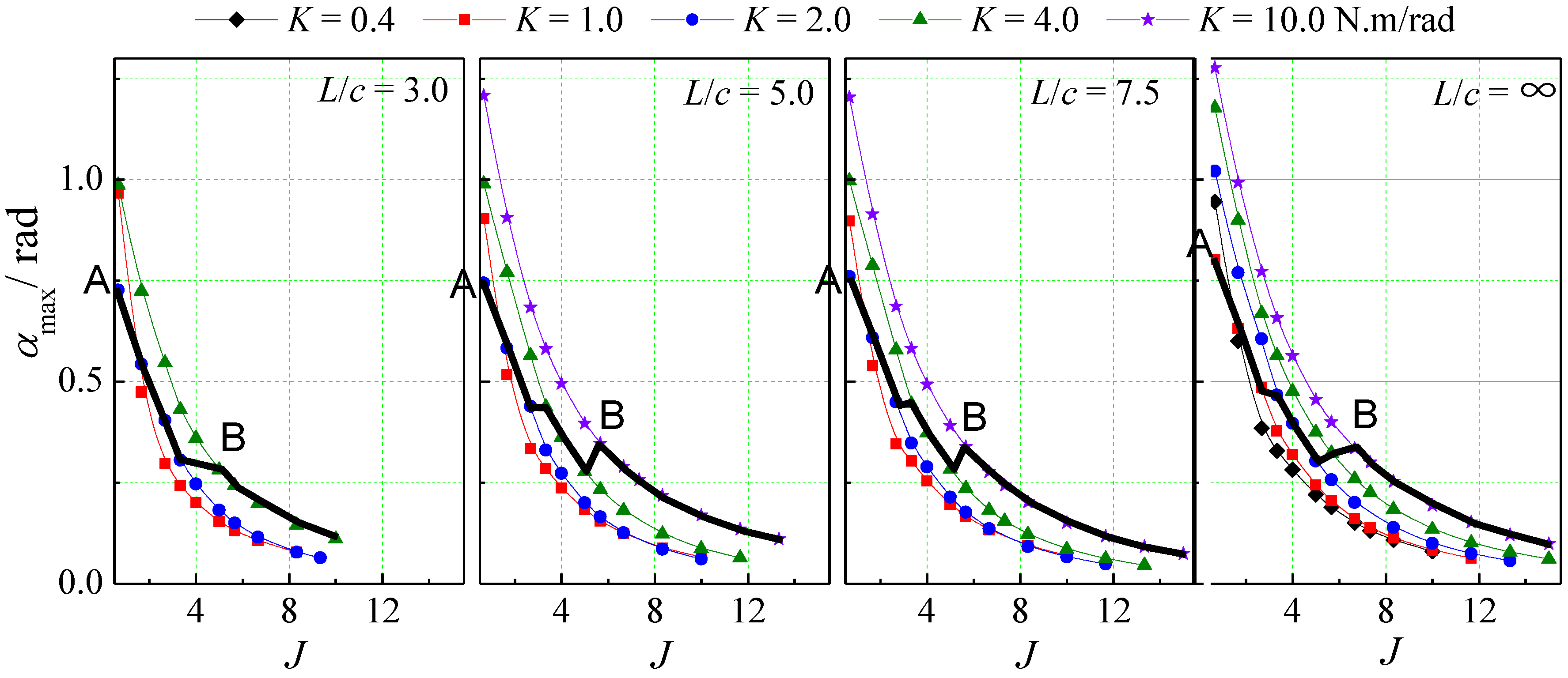
The maximum AoA under different working conditions is calculated and compared, as shown in Figure 9. As a whole, the αmax decreases with the advance coefficient, and with the increase in spring stiffness, the αmax under the same working condition gradually increases. This is also easy to understand, because with the increase in the spring stiffness, the hydrodynamic moment that the spring can resist is increasing, and the AoA increases with the increase in the hydrodynamic moment. As a result, the AoA of the flapping foil system is increasing. At the same time, the increase in swing arm length also increases the αmax under the same working condition. In order to analyze the relationship between αmax and KT, Figure 9 also depicts the αmax trajectory corresponding to the maximum thrust coefficient, as shown by the black solid line. It is obtained by comparing with the results of thrust coefficient in Figure 8. From the trajectory of this black line, it can be found that at a low advance coefficient (J = 0.67), the αmax corresponding to the maximum thrust coefficient is the smallest in all the different spring stiffness conditions, about 0.75 rad (the point A in the black solid line). That is, at a lower advance coefficient, the thrust generated by the flapping foil with smaller AoA is higher. However, at a higher advance coefficient (J ≈ 6), the highest thrust coefficient point has the maximum αmax in all different spring stiffness conditions, about 0.3 rad (the point B in the black solid line). That is, under the condition of high advance coefficient, the thrust generated by the semi-active flapping foil with larger AoA is higher. For the intermediate advance coefficient conditions (points between point A and point B), the αmax corresponding to the maximum thrust transits from a smaller value to a larger value step by step, which indicates that the αmax corresponding to the maximum thrust coefficient is almost centered. That is, when the advance coefficient is at the middle value, α Too large or too small αmax is not conducive to the generation of thrust. It can be understood that when the αmax is too large, there is obvious separation phenomenon on the flapping foil surface, which will not produce effective lift, thus affecting the generation of thrust. When the αmax is too small, the AoA decreases, the lift coefficient of the airfoil decreases, leading to reduced thrust. In addition, it can be observed that the jumping of the black solid line (αmax trajectory corresponding to the maximum thrust coefficient) between different spring stiffness roughly occurs in the range , which indicates that the maximum thrust tends to occur in the range of this AoA.
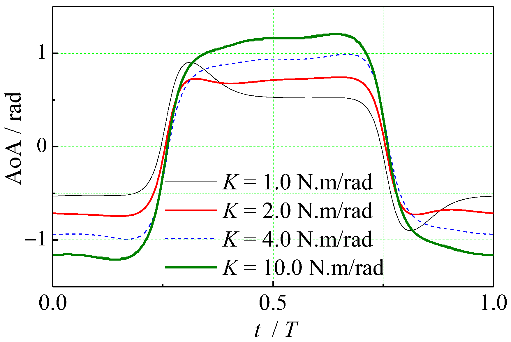
Meanwhile, a similar rule can be found from the comparison of the maximum AoA curves of flapping foil with different spring stiffness, as shown in Figure 9. Under the condition of low advance coefficient, the ability of the spring with small stiffness (e.g., ) to resist hydrodynamic torque is low, so the flapping foil works at a small AoA, resulting in higher thrust. At a higher advance coefficient, the relative flow velocity increases, and the hydrodynamic effect on the foil is enhanced. Therefore, the spring with higher stiffness (e.g., ) can resist the effect of hydrodynamic torque more strongly, so that the flapping foil can work at a larger AoA with higher thrust. However, the working condition at the lowest advance coefficient point (point A) in Figure 9 is a special case. Specifically, at the condition of the lowest advance coefficient point shown in the first three figures in Figure 9, the αmax of is greater than that of . In the last figure of Figure 9, the αmax of changes to the smallest one. It was found through inspection that this is due to a sudden increase in the AoA time-history curves at the low speed point under these conditions. Taking the working condition as an example, Figure 10 shows the time-history curve of AoA at low advance coefficient point (. It can be seen that, unlike the approximate sinusoidal AoA time-history curve of the conventional fully active flapping foil, the AoA time-history curve of this semi-active flapping foil driven by the swing arm is trapezoidal. This kind of trajectory has little effect on the maximum efficiency value of flapping foil, while it can maintain high efficiency with a relatively wider working range [16]. With the increase in spring stiffness, the AoA of the foil increases gradually. Whereas, in the process of direction changing of AoA, a convex peak appears on the curve of , which leads to the change in the maximum AoA, as shown in Figure 9. We speculate that the reason for the AoA jump-like phenomenon may be that when the advance speed VA is too small, the relative velocity angle of the foil changes abruptly.
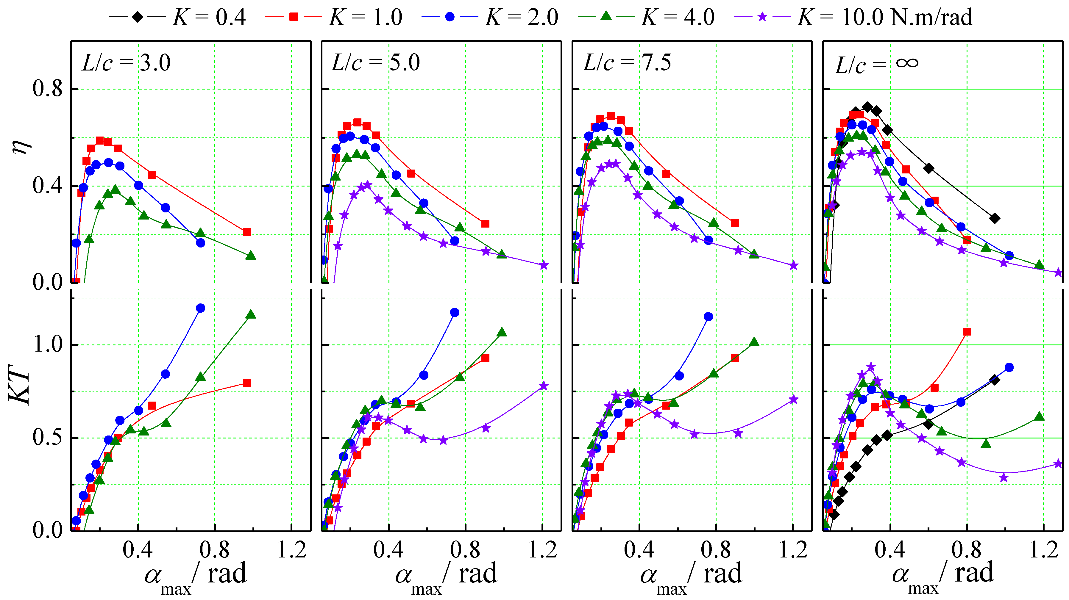
To further understand the relationship between efficiency, thrust coefficient, and maximum AoA, the comparison results of the performance curves of the flapping foil with different spring stiffness and different arm lengths are given in Figure 11. From the efficiency curves, we can find that with the increase in the swing arm, the maximum efficiency of each working condition increases gradually. The peak value of the highest efficiency decreases with the increase in the spring stiffness, which is consistent with the rule obtained in Figure 7, shown above. Most notably, the foil maximum AoA corresponding to the peak efficiency under different working conditions is very close, which is roughly concentrated near . It indicates that AoA is a key parameter affecting the efficiency of semi-active flapping foil propulsion, which has also been confirmed by previous studies of fully active and conventional semi-active flapping foils [14,16,17].
On the whole, the thrust coefficient curve in Figure 11 shows that, except for the condition of low advance coefficient, the peak thrust almost appears in the range , which is consistent with the conclusion obtained from the previous analysis in Figure 9. Read et al. [32] and Thaweewat [17] made a similar comparison in their work. The AoA corresponding to the peak efficiency point of the semi-active flapping foil is about 0.2 rad in their study. It can be seen from Figure 11 that, similar to the AoA characteristics of the conventional semi-active and the fully constraint foil systems, the peak efficiency of the semi-active flapping foil with an arc trajectory corresponds to a relative concentrated position. Compared with the conventional system, however, the peak efficiency point moves slightly to the right. That is, the maximum angle of attack corresponding to the peak efficiency point is about 0.3–0.4 rad, and unlike the spring stiffness’s influence on the peak efficiency, the spring stiffness has less influence on the peak thrust coefficient. Specifically, the thrust coefficient curve of different spring stiffness is slightly different. With the increase in spring stiffness, the thrust coefficient curve gradually shows a trend of first increasing and then decreasing. However, under the condition of high AoA (i.e., low advance coefficient), the law of thrust coefficient curve changing with AoA is uncertain, which needs further study.
The influence of swing arm length on the peak of the thrust coefficient is very clearly shown in Figure 11. Under the same spring stiffness, with the increase in swing arm length, the peak value of thrust coefficient increases gradually, but the thrust coefficient decreases more obviously at high AoA. It can be said that the increase in swing arm length can expand the influence of spring stiffness on thrust, which is consistent with the results in Figure 7, shown above. It is also certain that with the increase in the swing arm, the thrust coefficient curve is increasingly close to the curve of the conventional semi-active flapping foil.
4.3. Analysis of Vortex Structure
This section first compares the flow field of the flapping foil at low advance coefficient with different spring stiffness, and then analyzes the flow-field characteristics of thrust and efficiency peak points under the same spring stiffness.
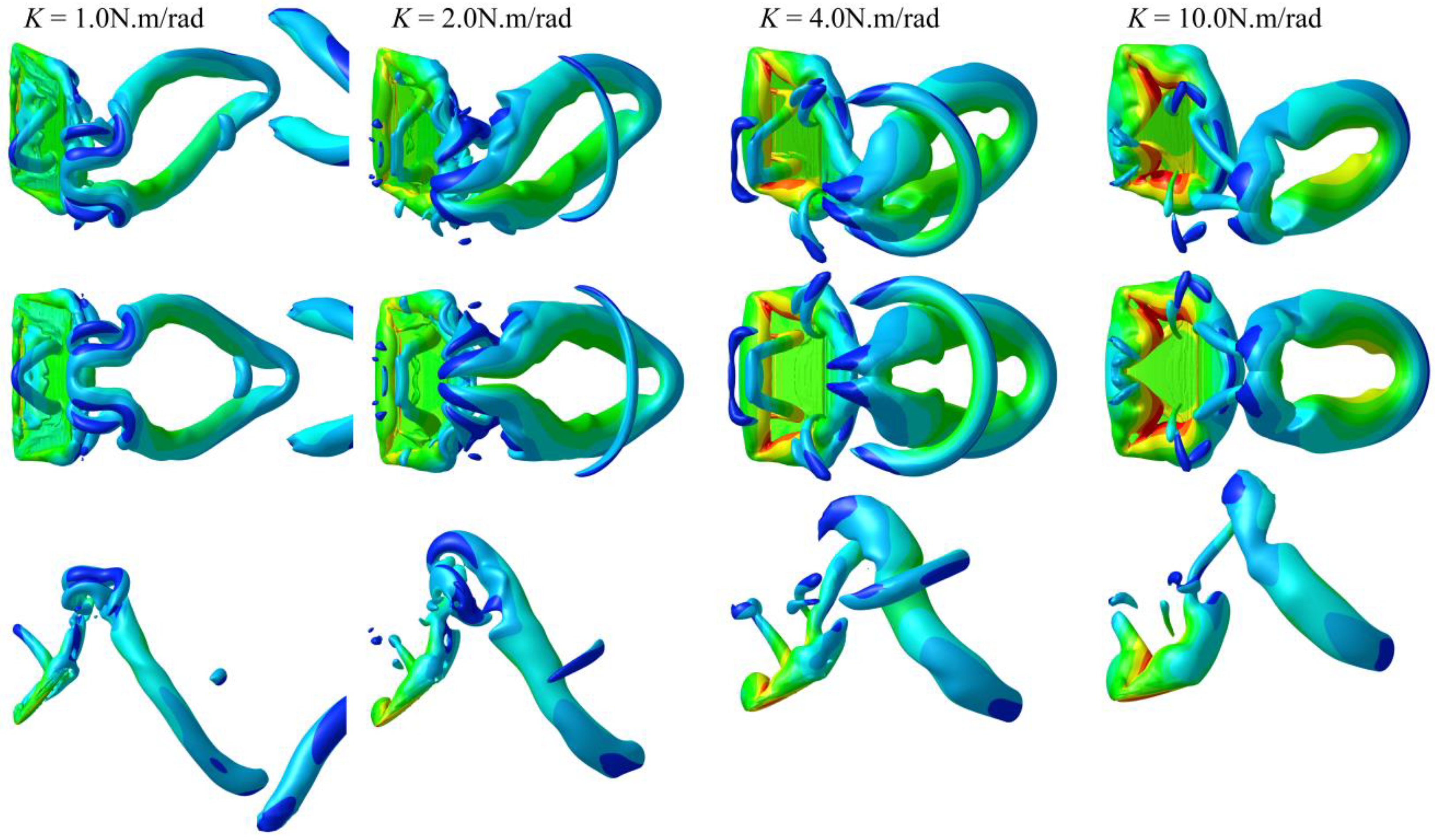
First, taking the working condition as an example, the flow separation of the flapping foil with different spring stiffness under the working condition of low advance coefficient is observed, as shown in Figure 12. The time selected in the figure is the time when the swing angle of the swing arm (β) is zero. The three lines of pictures in the Figure 12 are the structure of the separated vortex observed from three perspectives. From top to bottom, they are the aerial view, Y-plane view, and Z-plane view.
From the results in Figure 12, it is found that with different spring stiffness the flow on the flapping foil surface are all fully separated, and the flow-field structure of vortex ring interlocking appears under the working condition of low advance coefficient. Von Ellenrieder et al. [13] also observed this phenomenon on a flapping foil with an aspect ratio of 3. With the increase in spring stiffness, the swing wing surface separation becomes stronger, the separation area is larger, and the vortex system also diverges faster, and decays rapidly in the process of developing downstream. This may be the reason for the lower efficiency of the flapping foil at a low advance coefficient. From the horizontal comparison of the Z-plane view, the swing angle of the lower spring stiffness foil is larger, so the corresponding AoA is smaller. This is the reason why the thrust of the flapping foil with lower spring stiffness is higher at a low advance coefficient.
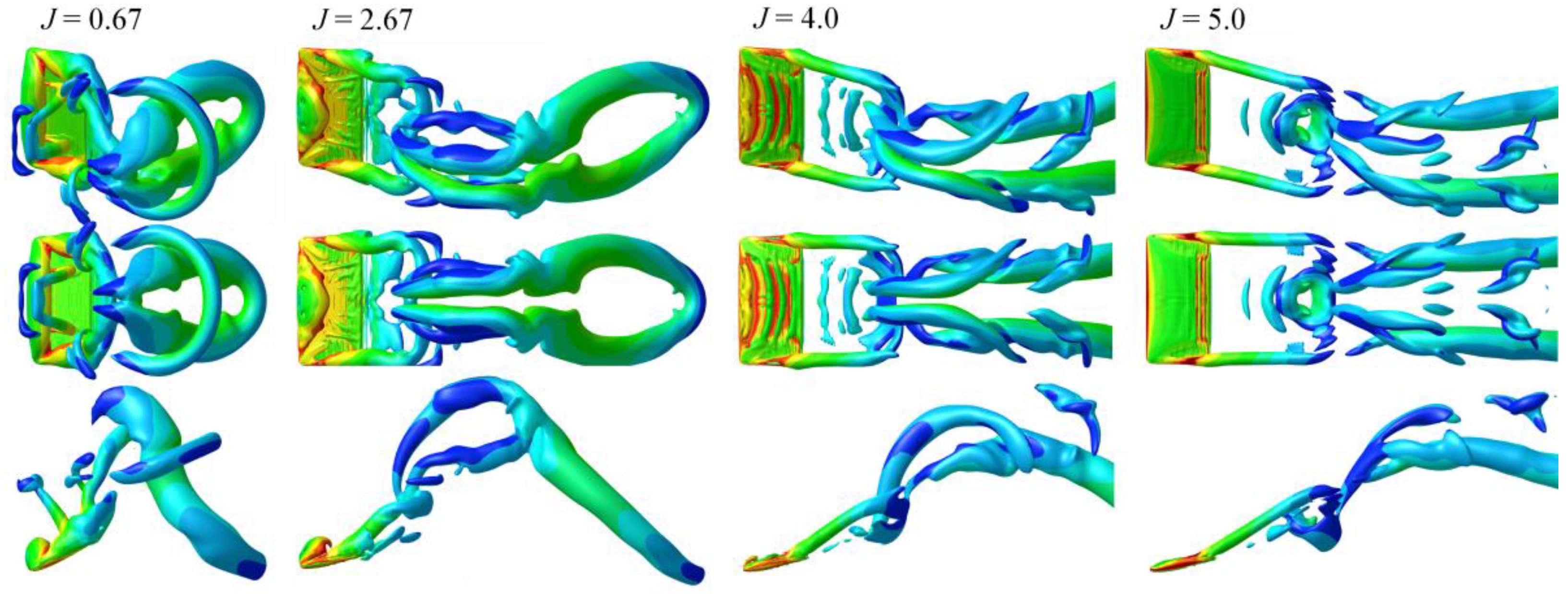
Then, under the condition of , the flow fields of the flapping foil near the starting point, the thrust valley point, the thrust peak point, and the efficiency peak point were further observed. The corresponding advance coefficients (J) of these four working conditions are 0.67, 2.67, 4.0, and 5.0, as shown in Figure 13. On the whole, the correlation of vortex ring structure in the wake of the flapping foil gradually weakens with the increase in advance coefficient. It can be seen from the figure that there are obvious vortex rings under the two working conditions, but the spatial correlation between adjacent vortex rings is weakened under working condition. In both cases, the wake is stretched along the flow direction due to the increase in advance speed, so there is no obvious vortex ring structure. However, in the process of developing downstream, taking the working condition as an example, the winding between the tip vortex and the separation vortex on the flapping foil surface can be seen clearly. Specifically, from the perspective of lateral comparison, the general development law of the trailing vortex of the flapping foil is shown as follows: first, the trailing vortex of the flapping foil shows a typical vortex ring structure. Then, with the increase in advance speed, the vortex ring is stretched, and spatial separation occurs between adjacent vortex rings, and the tip vortex and the separated vortex on the airfoil surface can be clearly distinguished gradually. With the further increase in the advance speed, the tip vortex and separation vortex almost develop independently at the beginning of their formation, and then intertwine with each other to form a complex wake field structure. From the perspective of the spatial position of the twining phenomenon, it roughly occurred at the moment when the flapping foil moved and reversed in the Y-direction. It is not difficult to find that the vortex ring is the result of the tip vortex and the separated vortex on the airfoil surface sticking together, while the vortex ring interlocking is formed by the compression of the vortex ring in space.
According to the thrust coefficient curve under the same conditions (), shown in Figure 8, corresponds to the valley point on the thrust coefficient curve. It can be seen from Figure 13 that under this working condition, the swing angle of the flapping foil is obviously small, leading to a reduction in the AoA and the lift coefficient of the airfoil; At the same time, there is a strong separation on the airfoil surface, which cannot produce effective lift, thus affecting the generation of thrust. That is to say, the lift generated by the airfoil surface and its contribution to the thrust are both very small under this working condition, which may be the reason for the thrust valley at this point.
5. Conclusions
In this paper, the flow field and motion of a circular-arc-track semi-active flapping foil driven by a swing arm under different arm lengths and spring stiffness are simulated. Its hydrodynamic performance, flow-field characteristics and motion characteristics are systematically analyzed. The flapping foil used in this study is a small aspect ratio NACA0012 airfoil, and a preliminary installation scheme on the vehicle is given, which is more consistent with the shape and engineering practicality requirements of the bionic propeller.
- The influence of arm length and spring stiffness on the performance of the semi-active flapping foil is very clear. Increasing the length of the swing arm is beneficial to improving the peak efficiency of this semi-active flapping foil with circular-arc trajectory. At the same swing arm length, reducing the spring stiffness is also conducive to improving the peak efficiency of the flapping foil. The analysis of the maximum angle of attack shows that there is a definite corresponding relationship between the maximum angle of attack and the peak efficiency. For the flapping foil with the small aspect ratio NACA0012 airfoil structure, its peak efficiency is usually concentrated near , and it can maintain high efficiency within a certain range of .
- The influencing factors of the thrust coefficient of the semi-active flapping foil propulsion are complex. The length of the swinging arm, the spring stiffness, and the advance coefficient can all have a significant impact on the thrust coefficient of the flapping foil. On the whole, compared with the conventional semi-active foil, the elliptical trajectory system also has a large thrust coefficient at low advance coefficient. The curve of the thrust coefficient decreases monotonically with the increase in advance coefficient when the spring stiffness is small. Under the condition of high spring stiffness, there is a peak value and a valley value of the thrust coefficient. According to the analysis of the flow field, the reason for the thrust valley may be the combined effect of the swing angle and the angle of attack. At the valley point of the thrust coefficient, the angle of attack of the flapping foil is large, so the vortex separation of foil is significant and the lift value is low. At the same time, the swing angle is small, so the contribution of lift to the thrust is low, which leads to the appearance of the thrust valley. In addition, by comparing the thrust coefficient and the maximum angle of attack , it is found that too large or too small is unfavorable to the thrust under the working condition of the intermediate advance stage, and the peak thrust tends to appear in the range .
- The flow-field analysis of the low aspect ratio airfoil shows that the vortex rings are interlocked in the wake field of the flapping foil at a low advance speed. With the increase in advance coefficient, the vortex rings are gradually lengthened first, and then separated from each other. When the advance coefficient is further increased, the vortex ring is split into a tip vortex and separated vortex on the airfoil surface. From the reverse analysis, the vortex ring is the result of the tip vortex and the separated vortex on the airfoil surface sticking together, while the vortex ring interlocking is formed by the compression of the vortex ring in space.
Author Contributions
Conceptualization, J.Z. and L.M.; methodology, W.Y.; investigation, J.Z. and L.M.; validation, W.Y.; writing—original draft preparation, J.Z. and L.M.; writing—review and editing, L.M. and W.S. All authors have read and agreed to the published version of the manuscript.
Funding
This research was funded by the National Natural Science Foundation of China (grant no. 51309070, 51503051), the Advanced Aviation Power Innovation Workstation Project (grant no. HKCX-2019-01-005, HKCX2020-02-024), and a Shandong Province Science and Technology Development Plan item (grant No. 2013GGA10065).
Conflicts of Interest
The authors declare no conflict of interest. The funders had no role in the design of the study; in the collection, analyses, or interpretation of data; in the writing of the manuscript, or in the decision to publish the results.
References
- Triantafyllou, M.S.; Triantafyllou, G.S. An efficient swimming machine. Scientific 1995, 272, 64–70. [Google Scholar] [CrossRef]
- Liu, H.X.; Su, Y.M.; Pang, Y.G. Numerical study on swing gliding swimming of tuna like underwater robot. Ship Mech. 2020, 24, 145–153. (In Chinese) [Google Scholar]
- Luo, Y.; Xia, Q.; Shi, G.; Pan, G.; Chen, D. The effect of variable stiffness of tuna-like fish body and fin on swimming performance. Bioinspiration Biomim. 2020, 16, 016003. [Google Scholar] [CrossRef] [PubMed]
- Esposito, C.J.; Tangorra, J.L.; Flammang, B.E.; Lauder, G.V. A robotic fish caudal fin: Effects of stiffness and motor program on locomotor performance. J. Exp. Biol. 2012, 215, 56–67. [Google Scholar] [CrossRef] [Green Version]
- Desvignes, T.; Robbins, A.E.; Carey, A.; Bailon-Zambrano, R.; Nichols, J.; Postlethwait, J.; Stankunas, K. Coordinated patterning of zebrafish caudal fin symmetry by a central and two peripheral organizers. Dev. Dyn. 2022, 251, 1306–1321. [Google Scholar] [CrossRef]
- Borazjani, I.; Sotiropoulos, F. Numerical investigation of the hydrodynamics of carangiform swimming in the transitional and inertial flow regimes. J. Exp. Biol. 2009, 211, 1541–1558. [Google Scholar] [CrossRef] [Green Version]
- Shen, H.Y.; Zhu, B.W.; Wang, Z.H.; Yu, Y.L. Study on propagation characteristics of deformed curvature waves of fish swimming in eel mode. Acta Mech. Sin. 2019, 51, 1022–1030. (In Chinese) [Google Scholar]
- Huang, Z.; Ma, S.; Bagheri, H.; Ren, C.; Marvi, H. The Impact of Dorsal Fin Design on the Swimming Performance of a Snake-Like Robot. IEEE Robot. Autom. Lett. 2022, 7, 4939–4944. [Google Scholar] [CrossRef]
- Cheng, X.; Guang, P.; Qiaogao, H. Performance Analysis of Airfoil Flow Field of a Mannequin-like Flexible Submersible. Digit. Ocean. Underw. Warf. 2020, 3, 265–270. (In Chinese) [Google Scholar]
- Wei, Z.; Hu, Y.; Long, W.; Jia, Y. Development of a flipper propelled turtle-like underwater robot and its CPG-based control algorithm. In Proceedings of the IEEE Conference on Decision & Control, Cancun, Mexico, 9–11 December 2008. [Google Scholar]
- Mannam, N.P.B.; Krishnankutty, P.; Vijayakumaran, H.; Sunny, R.C. Experimental and Numerical Study of Penguin Mode Flapping Foil Propulsion System for Ships. J. Bionic Eng. 2017, 14, 770–780. [Google Scholar] [CrossRef]
- Wu, X.; Zhang, X.; Tian, X.; Li, X.; Lu, W. A review on fluid dynamics of flapping foils. Ocean. Eng. 2020, 195, 106712. [Google Scholar] [CrossRef]
- Von Ellenrieder, K.D.; Parker, K.; Soria, J. Flow structures behind a heaving and pitching finite-span wing. J. Fluid Mech. 2003, 490, 129–138. [Google Scholar] [CrossRef]
- Anderson, J.M.; Streitlien, K.; Barrett, D.S.; Triantafyllou, M.S. Oscillating Foils of High Propulsive Efficiency. J. Fluid Mech. 1998, 360, 41–72. [Google Scholar] [CrossRef]
- Li, M.Y. Flow Mechanism Analysis and Experimental Study of Swing Wing Propulsion. Master’s Thesis, Harbin Institute of Technology, Harbin, China, 2019. [Google Scholar]
- Mei, L.; Zhou, J.; Yu, D.; Shi, W.; Pan, X.; Li, M. Parametric Analysis for Underwater Flapping Foil Propulsor. Water 2021, 13, 2103. [Google Scholar] [CrossRef]
- Thaweewat, N.; Phoemsapthawee, S.; Juntasaro, V. Semi-active flapping foil for marine propulsion. Ocean. Eng. 2018, 147, 556–564. [Google Scholar] [CrossRef]
- Schnipper, T.; Andersen, A.; Bohr, T. Vortex wakes of a flapping foil. J. Fluids Mech. 2009, 633, 411. [Google Scholar] [CrossRef] [Green Version]
- Andersen, A.; Bohr, T.; Schnipper, T.; Walther, J.H. Wake structure and thrust generation of a flapping foil in two-dimensional flow. J. Fluids Mech. 2017, 812, R4. [Google Scholar] [CrossRef] [Green Version]
- Kim, D.; Strom, B.; Mandre, S.; Breuer, K. Energy Harvesting Performance and Flow Structure of an Oscillating Hydrofoil with Finite Span. J. Fluids Struct. 2017, 70, 314–326. [Google Scholar] [CrossRef]
- Bøckmann, E.; Steen, S. Experiments with actively pitch-controlled and spring-loaded oscillating foils. Appl. Ocean. Res. 2014, 48, 227–235. [Google Scholar] [CrossRef]
- Yang, F.; Shi, W.; Wang, D. Systematic Study on Propulsive Performance of Tandem Hydrofoils for a Wave Glider. Ocean. Eng. 2019, 179, 361–370. [Google Scholar] [CrossRef] [Green Version]
- Zhou, J.; Yan, W.; Yu, D.; Pan, X.; Zhao, X. An adaptive angle of attack flapping foil propeller and its design method Invention. Patents 2021. (In Chinese) [Google Scholar]
- Xiao, Q.; Hu, J.; Liu, H. Effect of Torsional Stiffness and Inertia on the Dynamics of Low Aspect Ratio Flapping Wings. Bioinspiration Biomim. 2014, 9, 16008. [Google Scholar] [CrossRef] [PubMed] [Green Version]
- Phoemsapthawee, S.; Thaweewat, N.; Juntasaro, V. Influence of Resonance on the Performance of Semi-Active Flapping Propulsor. Ship Technol. Res. 2020, 67, 51–60. [Google Scholar] [CrossRef]
- Esfahani, J.A.; Barati, E.; Karbasian, H.R. Fluid structures of flapping airfoil with elliptical motion trajectory. Comput. Fluids 2015, 108, 142–155. [Google Scholar] [CrossRef]
- Zhang, Y.; Yang, F.; Wang, D.; Jiang, X. Numerical investigation of a new three-degree-of-freedom motion trajectory on propulsion performance of flapping foils for UUVs. Ocean. Eng. 2021, 224, 108763. [Google Scholar] [CrossRef]
- Mei, L.; Yan, W.; Zhou, J.; Yu, D.; Wu, P. Working characteristics of self-pitching flapping foil propulsor. MARINE 2021, 412. [Google Scholar] [CrossRef]
- Floc’h, F.; Phoemsapthawee, S.; Laurens, J.M.; Leroux, J.B. Porpoising foil as a propulsion system. Ocean. Eng. 2012, 39, 53–61. [Google Scholar] [CrossRef]
- Menter, F.R. Two-equation eddy-viscosity turbulence models for engineering applications. AIAA J. 1994, 32, 1598–1605. [Google Scholar] [CrossRef] [Green Version]
- Shenghao, Z.; Lei, M.; Junwei, Z. Numerical prediction of hydrodynamic performance of propeller with different shape swinging wings. Chin. J. Ship Res. 2021, 16, 50. (In Chinese) [Google Scholar]
- Read, D.A.; Hover, F.S.; Triantafyllou, M.S. Forces on oscillating foils for propulsion and maneuvering. J. Fluids Struct. 2003, 17, 163–183. [Google Scholar] [CrossRef]
- Schouveiler, L.; Hover, F.S.; Triantafyllou, M.S. Performance of flapping foil propulsion. J. Fluids Struct. 2005, 20, 949–959. [Google Scholar] [CrossRef]
Figure 1.
Simplified schematic of the semi-active flapping hydrofoil driven by the swing arm.

Figure 2.
Three-dimensional geometric shape of the flapping hydrofoil.

Figure 3.
Schematic diagram of the computational domain and gradual mesh refinement.

Figure 4.
Comparison of propulsive performance with different time steps.

Figure 5.
Comparisons of the propulsive efficiency η and the thrust coefficient cT with previous experimental results for amax = 20°.
Figure 5.
Comparisons of the propulsive efficiency η and the thrust coefficient cT with previous experimental results for amax = 20°.

Figure 6.
Comparison of the vorticity pattern visualized in the foil wake (). (Experimental results are from Figure 3c in Schnipper [18]).

Figure 7.
Propulsion efficiency curves with different arm length and different spring stiffness.

Figure 8.
Thrust coefficient with different arm length () and different spring stiffness (K).

Figure 9.
Maximum AoA with different spring stiffness and swing arm length. (black solid line is αmax trajectory corresponding to the maximum thrust coefficient).
Figure 9.
Maximum AoA with different spring stiffness and swing arm length. (black solid line is αmax trajectory corresponding to the maximum thrust coefficient).

Figure 10.
AoA time-history curve of the flapping foil with different spring stiffness for .

Figure 11.
Propulsive performance with different spring stiffness and swing arm lengths.

Figure 12.
Flow condition of the flapping foil with different spring stiffness ().

Figure 13.
The flow field and vortex structure of a flapping foil with different advance coefficients ().
Figure 13.
The flow field and vortex structure of a flapping foil with different advance coefficients ().


Table 1.
Parameters of the semi-active flapping hydrofoil with arc trajectory.
| Symbol | Units | Definition |
|---|---|---|
| VA | m/s | speed of the hull |
| T | s | period of the flapping hydrofoil |
| L/c | m | arm length |
| c | m | chord length of the flapping hydrofoil |
| H | m | spanwise of the flapping hydrofoil |
| R | m | radius of round corners designed at both ends of the span direction of the flapping hydrofoil |
| β | radian | swing angle of the swing arm |
| f | Hz | swing frequency of the swing arm |
| θ | radian | pitching angle of the flapping hydrofoil |
| Vrel,0 | m/s | pitching center speed of the foil relative to the hull |
| Vx0,Vy0 | m/s | velocity components of Vrel,0 |
| Fx0,Fy0 | m | X-direction force, Y-direction force exerted by the swing arm on the pitching center of flapping foil, respectively |
| Mz0 | N m | torque exerted by the swing arm on the pitching center of flapping foil |
| Mz | N m | fluid moment imposed on foil |
| K | Nm/rad | torsion spring stiffness |
| I | Kg m2 | rotational inertia about the axis of the flapping hydrofoil considering the attached water |
| N | average thrust in the forward direction | |
| α (AoA) | radian | angle of attack of flapping hydrofoil |
| St | St number of flapping hydrofoil | |
| J | advance coefficient | |
| KT | thrust coefficient | |
| η | propulsive efficiency of flapping hydrofoil |
Table 2.
Grid size and refinement scheme.
| Direction | Hydrofoil Surface Region | Refinement Area |
|---|---|---|
| spanwise/Z | ||
| chordwise/X | ||
| normal direction/Y |
Disclaimer/Publisher’s Note: The statements, opinions and data contained in all publications are solely those of the individual author(s) and contributor(s) and not of MDPI and/or the editor(s). MDPI and/or the editor(s) disclaim responsibility for any injury to people or property resulting from any ideas, methods, instructions or products referred to in the content. |
© 2023 by the authors. Licensee MDPI, Basel, Switzerland. This article is an open access article distributed under the terms and conditions of the Creative Commons Attribution (CC BY) license (https://creativecommons.org/licenses/by/4.0/).
Share and Cite
MDPI and ACS Style
Zhou, J.; Yan, W.; Mei, L.; Shi, W. Performance of Semi-Active Flapping Hydrofoil with Arc Trajectory. Water 2023, 15, 269. https://doi.org/10.3390/w15020269
AMA Style
Zhou J, Yan W, Mei L, Shi W. Performance of Semi-Active Flapping Hydrofoil with Arc Trajectory. Water. 2023; 15(2):269. https://doi.org/10.3390/w15020269
Chicago/Turabian StyleZhou, Junwei, Wenhui Yan, Lei Mei, and Weichao Shi. 2023. "Performance of Semi-Active Flapping Hydrofoil with Arc Trajectory" Water 15, no. 2: 269. https://doi.org/10.3390/w15020269
Note that from the first issue of 2016, this journal uses article numbers instead of page numbers. See further details here.